1

Forthcoming, European Economic Review

Global Banking and International Business Cycles

Robert Kollmann (*) ECARES, Université Libre de Bruxelles, Université Paris-Est and CEPR

Zeno Enders University of Bonn

Gernot J. Müller University of Bonn and CEPR

January 13, 2010

This paper incorporates a global bank into a two-country business cycle model. The bank collects deposits from households and makes loans to entrepreneurs, in both countries. It has to finance a fraction of loans using equity. We investigate how such a bank capital requirement affects the international transmission of productivity and loan default shocks. Three findings emerge. First, the bank's capital requirement has little effect on the international transmission of productivity shocks. Second, the contribution of loan default shocks to business cycle fluctuations is negligible under normal economic conditions. Third, an exceptionally large loan loss originating in one country induces a sizeable and simultaneous decline in economic activity in both countries. This is particularly noteworthy, as the 2007-09 global financial crisis was characterized by large credit losses in the US and a simultaneous sharp output reduction in the US and the Euro Area. Our results thus suggest that global banks may have played an important role in the international transmission of the crisis.

JEL codes: F3, F4, G2, G1 Key words: global banking, international business cycles, bank capital requirements, global financial crisis, credit losses. ------------------------------------ (*) Corresponding author: ECARES, CP 114, Université Libre de Bruxelles; 50 Av. Franklin Roosevelt; B-1050 Brussels, Belgium; robert_kollmann@yahoo.com

We are very grateful to two referees, and to our discussants Charles Engel, Victoria Hnatkovska, Stefano Neri, Philipp Schnabl and Andrew Scott for their advice. For useful suggestions we thank Mick Devereux, Domenico Giannone, Johannes Pfeifer, Bruce Preston, Werner Roeger, Stephanie Schmitt-Grohé, Martín Uribe, Skander Van den Heuvel and Michael Woodford. We also benefited from comments by workshop participants at the "Advances in International Macroeconomics--Lessons from the Crisis" conference (EU Commission, Brussels), Columbia University, Annual Meeting of the American Economic Association, Konstanz Seminar on Monetary Theory and Policy, Hungarian National Bank, and Vienna Institute for Advanced Studies. Kollmann thanks the National Bank of Belgium and the EU Commission for financial support (CEPR project 'Politics, Economics and Global Governance: The European Dimensions' funded by the EU Commission under its 7th Framework Programme for Research.) The quantitative model presented here draws heavily on Robert Kollmann’s manuscript ‘Banks and the Domestic and International Propagation of Macroeconomic and Financial Shocks’ (May 2010).

2

1. Introduction During the recent (2007-2009) financial crisis, economic activity collapsed simultaneously in the United States and in the Euro Area (EA). This is striking as, typically, the US business cycle leads the EA business cycle. Several indicators suggest that the crisis was triggered by specific developments in the US. House price indices, for instance, started to plummet by mid-2006 in the US, but have been holding up well in the EA (ECB, 2010). In addition, while both US and EA banks suffered large loan losses, almost all losses experienced by US banks were due to domestic loans, whereas the credit losses of EA banks were largely due to foreign (US) loans (IMF, 2010). This paper assesses under what circumstances country-specific shocks trigger a sharp and highly synchronized international downturn. We address this issue, using a quantitative international business cycle model. While standard macro models developed before the global financial crisis mostly abstracted from financial intermediaries, our model features a globally integrated banking sector.1 This allows us to account for financial factors in international economic fluctuations. Our model represents a two-country world, where each country is inhabited by a worker and an entrepreneur. The worker provides labor to the local entrepreneur and deposit savings at a globally operating bank, which lends to entrepreneurs in both countries. Entrepreneurs accumulate capital and produce a homogenous tradable good using capital and labor. We focus on the role of bank capital for the international transmission of macroeconomic and financial shocks. In order to do so, we maintain an aggregate perspective and assume a representative bank, i.e., we abstract from the interbank market, where liquidity shortages can emerge as an additional friction in financial intermediation.2 Specifically, we assume that the bank has to finance a fraction of the loans using its own funds (equity). We are agnostic as to whether this constraint reflects regulatory requirements or, more broadly, market pressures.3 In equilibrium, the loan rate exceeds the deposit rate; and the interest spread is a decreasing function of the bank's 'excess' capital, i.e., of bank capital held in excess of the target level. We assume exogenous fluctuations in productivity and loan default rates, and calibrate the model to US and EA data. Considering the period 1995-2010, we show that the model is able account for key features of economic fluctuations, including the co-movement of macroeconomic aggregates across the US and the EA, as well as the behavior

1 Krugman and Obstfeld (2008) point out that ‘one of the most pervasive features of today’s banking industry is that banking activities have become globalized.’ The growing international orientation of US banks is, e.g., documented in Acharya and Schnabl (2009), and in Cetorelli and Goldberg (2008) who report that global US banks (banks with positive assets from foreign offices) held 70% of US banking system assets in 2005 (the share of assets from foreign offices within total assets of US global banks exceeded 20% in 2005). External assets and liabilities of US banks (each) represented about 30% of US GDP at the end of September 2009; for Germany, France and the UK, external bank assets and liabilities represent more than 100% of domestic GDP (BIS, 2010). 2 Disruptions in the interbank market played an important role in the early stages of the global financial crisis (Brunnermeier (2009)); see Gertler and Kiyotaki (2010) for a formal treatment of the interbank market. 3 Traditionally, regulating banks' capital is often justified by limiting moral hazard in the presence of informational frictions and deposit insurance, see Dewatripont and Tirole (1994). In the present paper we abstract from these issues. Our focus, instead, is on the business cycle implications of bank capital requirements, which we take as given. Finally, we note that our representative global bank may be thought of in more general terms as the global financial sector. “Shadow banks” and other financial institutions too are key players in world financial markets. Yet net worth is an important determinant for all of these actors, whether they are officially classified as “banks” or not.

3

of financial variables such as loan and deposit volumes, and loan-deposit interest rate spreads. Model simulations show that the bank capital requirement is of little consequence for the international transmission of technology shocks. Moreover, country-specific technology shocks do not generate synchronized international output fluctuations in the set-up here, consistent with similar findings for conventional multi-country models (e.g., Backus et al. 1992). Our model simulations suggest that the contribution of loan default shocks to business cycle fluctuations is negligible under normal economic conditions. However, the calibrated model predicts that an exceptionally big credit loss in one country, of the magnitude seen in the US during the 2007-2009 recession, triggers a large and persistent decline in domestic and foreign output, by about 2% on impact. To understand this result, note that a loan loss reduces the global bank’s capital; due to the bank capital constraint, this raises domestic and foreign loan spreads, thus lowering lending, investment and output in both countries.4 By contrast, a loan loss shock has virtually no effect on loan spreads and output, in model variants without a bank capital requirement. The closed economy macro literature has only recently started to develop quantitative dynamic models with banks; see Goodfriend and McCallum (2007) for an early contribution. Aikman and Paustian (2006), Van den Heuvel (2008), de Walque et al. (2009), Angeloni and Faia (2009) and von Peter (2009) use closed economy general equilibrium models to analyze the macroeconomic implications of bank capital requirements. Cúrdia and Woodford (2009), Roeger (2009), Dib (2010), Gerali et al. (2010) and Meh and Moran (2010) embed banks in fairly rich, but closed economy DSGE models. Gerali et al. (op.cit.) estimate their model on time-series data for the EA and find that shocks to bank capital may have sizeable effects on economic activity. Our paper has been written independently of a complementary study by Iacoviello (2010) who presents a closed economy model in which banks, as well as entrepreneurs and impatient households face collateral constraints. He shows that a loan default by impatient households may trigger a sizeable recession, if the bank faces a capital requirement. International business cycle models have likewise largely abstracted from banks. An exception is Olivero (2010) who studied the implications of a global, imperfectly competitive banking sector for international co-movements; in her analysis, banks do not face a capital requirement. Some recent open-economy studies consider a range of financial factors in order to explain the recent global recession. Mendoza and Quadrini (2010) simultaneously analyze financial globalization and spillovers of country-specific shocks to bank capital. In their two-country model, countries are characterized by different stages of financial development, determining the extent to which households can insure themselves against idiosyncratic income risk; in contrast to our paper, these authors do not study business cycles, as they assume that aggregate capital and production are constant.5 In a related contribution, Devereux and Yetman (2010) abstract from capital accumulation, banks, and financial shocks, but focus on the international transmission of productivity shocks in the presence of international portfolio holdings by 4 This mechanism is consistent with empirical results by Puri et al. (2010) who show, using German data for 2006-08, that lending was reduced by those retails banks which were particularly exposed to loan losses in the US. Similarly, Cetorelli and Goldberg (2010) identify international banking linkages as a determinant of a reduction in loan supply in emerging market economies after 2007. Our model assumes that a generic entrepreneur in each country borrows from the global bank, and (partially) defaults on bank loans. As our focus is on the international transmission of default shocks, we do not provide a detailed analysis of their origins, which arguably would require an explicit model of the housing sector (see Iacoviello (2010)). 5 After the present research was completed, several quantitative two-country DSGE models with banks were brought to our attention: Correa et al. (2010), Davis (2010) and Ueda (2010); these authors do not consider the international transmission channel (via a bank capital requirement) discussed here.

4

leverage-constrained investors; these authors find that, under a high level of financial integration, binding leverage constraints may induce a strong degree of cross-country output co-movement. Finally, Dedola and Lombardo (2010) and Perri and Quadrini (2010) model financial frictions by assuming that firms face borrowing constraints, as debt contracts are imperfectly enforceable; in their settings, a country-specific 'credit shock' (tightening of borrowing constraint), may lead to a decline in global economic activity. Against this background, our contribution is to show how a country-specific loan loss triggers a worldwide recession in the presence of a global bank that faces a capital requirement. We do so within a quantitative business cycle model which captures key features of actual time-series data. However, in order to illustrate the underlying mechanism as transparently as possible, our analysis abstracts from various frictions which are often considered within larger DSGE models; in particular, we assume that only the bank faces a collateral constraint. 6 Our paper is therefore not meant to provide a complete quantitative account of the global financial crisis. Instead, it is complementary to the studies discussed above. The remainder of the paper is organized as follows. Section 2 discusses the data which motivate our investigation. Section 3 describes the model. Section 4 presents the quantitative results. Section 5 concludes. 2. Properties of US and EA macroeconomic data Our goal is to account for key features of US and EA business cycles. Figure 1 shows HP filtered quarterly log real GDP, and demeaned year-on-year (yoy) GDP growth rates, for the US (solid lines) and EA (dashed lines). The sample period is 1975q1-2010q1. (See Appendix for data definitions and sources.) Shaded areas indicate US recessions (according to the NBER). Figure 1 shows that the US cycle has tended to lead the European cycle by a few quarters--with the exception of the latest recession during which output collapsed simultaneously in the US and the EA (see Giannone et al. (2010) for detailed analyses of US-EA macro linkages). We argue below that this key feature of the 2007-2009 recession might be due to a credit loss shock to the globalized financial sector. Figure 2 illustrates important financial aspects of the 2007-2009 recession.7 The upper left panel shows quarterly time series for loan loss rates of US banks, and of German banks (taken as a proxy for loan loss rates of EA banks, as aggregate EA loan loss data are not available). The loss rates are expressed as annualized percentages of outstanding stocks of loans. The Figure shows that loan loss rates have reached unprecedented levels in 2007-2009. Note that the increase in loss rates was larger for US banks. According to estimates by the IMF (2010), the total worldwide bank writedowns on loans and securities during 2007-2009 amounted to 2,300 billion USD with about 70% due to loan losses. US and EA banks faced loan losses totaling 588 billion and 440 billion, respectively, according to the IMF estimates. (The ECB has conducted independent calculations, and reports similar figures; see ECB, 2010.) Importantly, losses on foreign loans account for less than 10% of the total loan losses experienced by US banks, while losses on foreign loans represent 60% of the credit losses of EA banks. The total credit losses of US banks represent about 4% of annual US GDP (14 trillion USD in 2007). Under the plausible assumption that a substantial share of the foreign loan losses of EA banks represents losses originating in the US, the total credit losses

6 Our analysis abstracts from of other issues which may also have played a quantitatively important role, in 2007-2009. Examples are oil and commodity price changes, and the zero lower bound (on the nominal interest rate) which constrained monetary policy. 7 Figure 2 plots data for 1995q1-2010q1 (shorter sample, due to lack of earlier synthetic EA data).

5

originating in the US amount to about 5% of annual US GDP. Below we explore the consequences of a 'loan-default shock' of this size in our quantitative model. The upper right panel of Figure 2 plots time series for the ratio of bank capital to bank assets, i.e. the ‘bank capital ratio’, for the US (solid line) and the EA (dashed line), based on accounting measures of bank equity.8 The bank capital ratios held up fairly well during the recent crisis—but it has been argued that this may partly reflect accounting discretion which has allowed banks to overstate the value of their assets in the crisis (e.g., Huizinga and Laeven 2009). Figure 2 therefore also plots time series for market prices of US and EA bank equity (Dow Jones bank index; Stoxx Europe 600 Banks); those prices have dropped sharply during the global recession--much more sharply than broad stock market indices (S&P 500; Stoxx Europe). Interestingly, US and EA bank stocks started to decline before the overall market. (All stock indices in Figure 2 are normalized to 100 in 2009q1.). This pronounced and early relative fall in bank stocks distinguishes the current recession from other post-war recessions—and suggests that banking problems were a key aspect of the global recession. Finally, Figure 2 also plots real loan growth rates (year-on-year), and bank lending rate spreads (in % per annum), for the US and the EA. At the beginning of the global recession, loan growth was still positive, but declined substantially towards the end of the recession; by mid-2009 aggregate US and EA lending contracted sharply. US and EA lending rate spreads started to rise strongly in late 2008.9 Below, we will assess whether our model matches US and EA business cycles, as described by second moments of HP filtered quarterly macroeconomic data. Table 1 reports key business cycle statistics for 1995q1-2010q1. The first two columns of the Table report standard deviations for output, consumption, investment, employment, deposits, loans, and the loan rate spread, both for the US and the EA. The other columns report correlations with domestic output, and correlations between US and EA variables. Table 1 confirms the well known fact (e.g., King and Rebelo, 1999) that consumption and employment are less volatile than GDP, while investment is more volatile. Deposits are somewhat less volatile than GDP, while loans are more volatile. The loan spread is roughly 20%-30% as volatile as (detrended) GDP. Empirically, investment and consumption are highly procyclical. This holds for loans as well, while loan spreads are countercyclical. EA deposits are acyclical. US deposits appear to be countercyclical, but this finding is not robust with respect to the sample period—in a longer sample (1975-2010) US deposits are weakly procyclical. All variables considered here exhibit strong cross-country correlations. Interestingly, in our sample the cross-country correlation of output is somewhat lower than that of consumption and investment.

3. The Model We consider a world with two countries, called Home and Foreign. In each country there is a representative worker and an entrepreneur. In addition there is a representative global bank. All agents are infinitely lived. The bank collects deposits from Home and Foreign workers, and makes loans to Home and Foreign entrepreneurs. There is a final good, produced by Home and Foreign entrepreneurs using local labor and capital. The good can

8 Note that we divide bank equity by total assets, and not by risk-weighted assets. The capital ratio of US banks is larger than that of EA banks, which reflect differences in the risk structure of US and EA banks’ assets, and in accounting standards. (We thank Skander Van den Heuvel for advice on these issues.) 9 We measure spreads as difference between bank loan rates and money market rates. We view this as a proxy for spreads between loan rates and deposit rates (there are no time series for US deposit rates).

6

be traded freely. It is used for consumption by all agents, and for capital accumulation by entrepreneurs. All markets are competitive. Our analysis centers on the role of a bank capital requirement for the transmission of shocks. We model that capital requirement as a flexible collateral constraint faced by the global bank--it bears a resource cost when deposits fall below a fraction of the bank assets. In order to focus sharply on the effect of this constraint, we assume that workers and entrepreneurs do not face collateral constraints.10 Preferences and technologies have the same structure in both countries. The following exposition thus focuses on the Home country. Foreign variables are denoted by an asterisk. 3.1. Agents and Markets The Home worker The Home worker consumes the final good, provides labor to the Home entrepreneur and invests her savings in one-period bank deposits. Her date t budget constraint is: 1

Dt t t t t tC D W N D R�� � � , (1)

where tC and tW are her consumption and the wage rate, respectively (the final good is used as numéraire). tN are hours worked. 1tD � is the bank deposit held by the Home

worker at the end of period t. DtR is the gross interest rate on deposits, between t-1 and t

( DtR is set at t-1). The Home worker’s expected life-time utility at date t is:

10[ ( ) ( ) ]s D N

t t s t s t ssE u C u D N��

� � � ��� � � �� � , (2)

where , 0D N� � are parameters. 1( ) ( 1)/(1 )u x x � ��� � � with 0� is an increasing and concave function (when 1,� � we set ( ) ln( )u x x� ). 0 1�� � is a subjective discount factor. Workers, entrepreneurs and the banker have the same subjective discount factor. Note that we assume that deposits provide utility to the worker (liquidity services). This allows us to calibrate the model in such a way that, in steady state, the deposit rate is smaller than the lending rate, and that workers hold deposits while entrepreneurs borrow.11 An alternative setup consistent with a positive loan spread and positive deposits is that workers are more patient than entrepreneurs and the banker. Such a setup allows to dispense with the assumption that deposits provide liquidity services; it delivers very similar results as the ‘deposits-in-utility’ framework discussed here. The Home worker maximizes (2) subject to the period-by-budget constraint (1). Ruling out Ponzi schemes, that decision problem has these first-order conditions: 1 1 1'( )/ '( ) '( )/ '( ) 1D D

t t t t t tR E u C u C u D u C�� � �� � � , '( ) Nt tu C W � � .

The Home entrepreneur The Home entrepreneur accumulates physical capital and uses capital and local labor to produce the final good. Home final good output, denoted ,tZ is produced using the Cobb-

10 Our structure thus differs from models with financial frictions in the tradition of Kiyotaki and Moore (1997). In those models there are no financial intermediaries; entrepreneurs are less patient than workers, and face a collateral constraint for debt, which ensures existence of a stationary equilibrium. 11 For simplicity, we assume that the (sub-)utility functions of consumption and deposits have the same CRRA form. This follows the typical ‘money-in-the-utility-function’ specifications used in the macro literature (deposits represent ‘money’ in our model); e.g., Obstfeld and Rogoff (1996), p.661. Our results do not hinge on this assumption (see below).

7

Douglas technology 1( ) ( ) ,t t t tZ K N � �� with 0 1. � � tK is the capital stock used at t. Home TFP t� is an exogenous random variable that follows an AR(1) process (see below). The law of motion of the Home capital stock is 1 (1 ) ,t t tK K I�� � � � where 0 1�� � is a depreciation rate and tI is gross investment. Gross investment is generated using the final good. Let ( )tI� be the amount of the final good needed to generate ,tI with ( ) ,t tI I� �

( ) 0, "( ) 0.' t tI I� � � The Home entrepreneur’s period t budget constraint is:

11 1(1 ) ( (1 ) ) ( ) ( )L L E

t t t t t t t t t t t tL R K K W N d L K N � � � � �� �� � � � � � � � , (3)

where tL is a one-period bank loan received by the Home entrepreneur in period t.

0 1Lt�� � is an exogenous stochastic loan default rate: at t, the entrepreneur only pays

back a fraction 1 Lt�� of the contracted amount ,L

t tL R where LtR is the (contractual)

gross loan rate between t-1 and t. LtR is set at t-1, while L

t� is realized at t. In stochastic model simulations discussed below, we assume that the default rate is autocorrelated and that its innovations are correlated with innovations to total factor productivity (according to empirical estimates). E

td is the entrepreneur’s dividend income at t. The entrepreneur consumes her

dividend income. Her expected lifetime utility at t is 0

( ),s Et t ss

E d� ���� with

1( ) ( 1)/(1 ),E Ex x �� ��� � � 0E� (when 1,� �� we set ( ) ln( )x x� � ). Maximization of that

life-time utility subject to (3) yields these first-order conditions: (1 )t t t tW K N � �� � ,

1 1 1(1 ) '( )/ '( ) 1L L E Et t t t tR E d d� �� �� � �� � , (4)

1 11 1 1 1 1( '( )/ '( )){ (1 )} 1/E E

t t t t t t t tE d d K N q q � � � � �� �� � � � �� � � ,

where 1'( (1 ) )t t tq K K� ��� � � is the marginal cost of gross investment at date t.

The global bank In period t, the global bank receives deposits 1tD � and *

1tD � from the Home and Foreign

workers, respectively, and makes loans 1tL � and *1tL � to the Home and Foreign

entrepreneurs. Let *1 1 1

Wt t tD D D� � �� � and

*1 1 1

Wt t tL L L� � �� � be worldwide stocks of deposits and

loans at the end of period t. The bank faces a capital requirement: her date t capital

1 1W Wt tL D� �� should not be smaller than a fraction � of the bank’s assets 1.

WtL � One may view

this as a legal requirement, or as an implicit requirement reflecting market pressures.12 We assume that the bank can hold less capital than the required level, but that this is costly (e.g., because the bank then has to engage in creative accounting). Let

12 We take the capital requirement as given, and focus on its macroeconomic effects. A large literature discusses micro-economic justifications for bank capital requirements (see Freixas and Rochet (2008)). That literature stresses that bank capital requirements can reflect market pressures. Essentially, capital require-ments help ensure that the banker acts in the interest of her creditors. A simple story, in the spirit of Kiyotaki and Moore (2005), is that the banker can walk away with a fraction � of the bank’s assets without pro- secution (and start a new life next period). Incentive compatibility then requires that the banker’s own funds (invested in the bank) may not fall below the assets with which the banker can abscond: 1 1 1.

W W Wt t tL D L�� � �� �

8

1 1 1( )W W Wt t t tx L D L�� � �� � � � 1 1(1 ) W W

t tL D� � �� � denote the bank’s ‘excess’ capital at the end of period t. The bank bears a cost ( )tx� as a function of .tx � is a convex function ( '' 0)� � for which we assume: ( ) 0tx� for 0tx � ; (0) 0.� � Thus, for 0tx � the bank incurs a positive cost. The cost is zero when the bank meets its capital requirement.13 At time t, the bank also bears an operating cost 1 1( , )W W

t tD L� �� � 1 1W W

D t L tD L� �� �� that is increasing and linear in deposits and loans, i.e. , 0D L� � (we assume that marginal operating costs are time-invariant). The bank’s period t budget constraint is: * * *

1 1 1 1 1 1( , ) ( (1 ) ) (1 ) (1 ) ,W W D W W W W B L L L L Wt t t t t t t t t t t t t t tL D R D L L D d L R L R D� � � �� � � � � �� �� � � � � � � � � � (5)

where Btd is the profit (dividend) generated by the bank at t. L

tR and *LtR are the gross

interest rates between t-1 and t on loans made to the Home and Foreign entrepreneurs, respectively (Home and Foreign loan rates differ as loan default rates differ across countries). The banker does not have access to other assets, and thus she consumes her dividends. Her expected life-time utility at t is:

0( )s B

t t ssE u d��

�� .The banker maximizes life-time utility subject to (5). Ruling out Ponzi schemes, that problem has these first-order conditions: 1 1'( )/ '( ) 1 'D B B

t t t t D tR E u d u d� �� � � � � � (6)

1 1 1(1 ) '( )/ '( ) 1 (1 ) 'L L B Bt t t t t L tR E u d u d� � � �� � �� � � � � � , (7)

* *1 1 1(1 ) '( )/ '( ) 1 (1 ) 'L L B B

t t t t t L tR E u d u d� � � �� � �� � � � � � , (8)

with 1 1' '((1 ) )W Wt tt L D� � � � �� � � . By accepting more deposits at t, the banker can increase her

date t consumption, at the cost of a reduction of consumption at t+1. Specifically, when the bank raises deposits 1

WtD � by 1 unit (holding constant loans), she incurs a marginal

operating cost ,D� and her (excess) capital falls by one unit. Hence, the banker’s

marginal benefit of deposits (in utility terms) is '( ){1 '}.St D tu d ��� � The discounted

expected marginal cost of deposits to the bank is 1 1 1'( )D Bt t tR E u d�� � � . At a maximum of the

bank’s decision problem, the expected marginal benefit equals the marginal cost (see eq. (6)). If the bank raises Home loans by one unit at t (holding constant deposits), then this lowers her date t dividend by 1 (1 ) ' .L t� ��� � � The bank’s effective (gross) real rate of

return on loans to the Home entrepreneur is thus 1 1(1 )/{1 (1 ) '},L Lt t L tR � � �� �� �� � � which

explains the Euler equation (7) (the same logic explains (8), which together with equation (7) implies a no-arbitrage condition between the effective return on loans to entrepreneurs in both countries; see below).

Market clearing, definition of GDP Market clearing for the final good requires: * * * *

1 1 1 1( ) ( ) ( , ) ( (1 ) )E E B W W W Wt t t t t t t t t t t t tZ Z C C d d d I I D L L D� � � �� � � �� � � � � � � � � � � � � . (9)

13 de Walque et al. (2009), Gerali et al. (2010) and Roeger (2009) assume a quadratic cost function

212( ) ( ) ,t tx x� �� under which the bank also bears a cost when 0.tx This function satisfies our assumptions.

Our setup is more general, as it is allows for the possibility that positive excess capital generates a convenience yield ( ( ) 0tx� � for 0tx ). Up to a linear approximation (around x=0) both specifications yield the same predictions (in particular, the loan spread is decreasing in tx if and only if ''(0) 0;� see below).

9

We assume that the bank purchases the resources that are necessary for Home deposits and Home lending, 1 1( , ),t tD L� �� from the Home final good producer, and that 50% of the resource cost ( )tx� is borne in Home final good units. As � and � are physical inputs used by the banking firm, they have to be subtracted from final good production when computing GDP. Hence, Home GDP, denoted by ,tY is:

11 1 1 12( , ) ( (1 ) )W W

t t t t t tY Z D L L D� �� � � �� �� � � � . (10) This definition of GDP ensures that world GDP equals world consumption (by all agents) plus world physical investment. Our calibration (see below) uses an investment cost function � such that ( )t tI I� � holds up to a first order approximation. Hence, the final good market clearing condition (9), and (10) (and the counterpart of (10) for the Foreign country) imply, up to first order: * * * *.E E B

t t t t t t t t tY Y C C d d d I I� � � � � � � � 3.2. Discussion Loan rate spreads and bank capital As deposits provide liquidity services to workers, and as financial intermediation is

costly, the deposit rate is lower than the loan rate. Let �1 1 1(1 )L L Lt t t tR R E �� � �� � and

�* * *1 1 1(1 )L L L

t t t tR R E �� � �� � be the expected effective gross interest rates (i.e. loan rates, net of the expected default rate) on loans to the Home entrepreneur and to the Foreign entrepreneur, respectively. Up to a certainty-equivalent approximation, the bank’s Euler equations (7)-

(8) imply � �*1 1

L Lt tR R� �� , i.e. that expected effective loan rates are equated across

countries.14 Furthermore (from (6) and (7)): �1 1/ {1 (1 ) }/{1 } 0' 'L Dt t L t D tR R � � �� � � �� � � �� � ,

which implies that approximately:

�1 1 (0) (0)' ''L Dt t D L tR R x�� ��� �� �� �� � � � , (11)

where a linear approximation of ( )' tx� around 0tx � was used, ( ) (0) (0)' ' ''t tx x� � �� � � (below, we assume that excess bank capital is zero in steady state). Hence, a rise in

excess bank capital 1 1(1 )W Wt t tx L D�� �� � � lowers the (effective) loan rate spread �1 1

L Dt tR R� ��

when the cost of excess capital is strictly convex, 0.''� Up to a certainty-equivalent (linear) approximation, the bank’s supply of loans and the entrepreneurs’ demand for loans at date t depend on the expected effective loan

rate �1LtR � , and not on the contractual loan rates *

1 1,L Lt tR R� � per se (see Euler equations

(4),(7),(8)). Hence shocks to expected default rates *1 1,L L

t t t tE E� �� � have no effect on �1LtR �

--and no effect on consumption, output, loans or deposits; such shocks only affect the contractual loan rates (when the expected Home default rate rises by 1 percentage point, the Home contractual loan rate 1

LtR � rises by approximately 1 percentage point as well, so

14 In the model, the contractual loan rates *

1 1,L Lt tR R� � differ across countries, when expected default rates

differ across countries. Contractual loan rates, and spreads between those rates and deposit rates, are highly positively correlated across the US and EA--the model matches those empirical correlations (see below).

10

that �1LtR � remains unchanged). Only unanticipated default rate changes induce wealth

transfers between entrepreneurs and banks, and affect the real economy.15 An unanticipated increase in the date t Home loan default rate brings about a wealth transfer from the bank to the Home entrepreneur. This lowers the bank’s capital. As shown below, the wealth transfer can have a sizable negative effect on world output,

when '' 0,� as the shock then raises the effective loan rate spread �1 1L Dt tR R� �� in both

countries, by the same amount (due to the no-arbitrage condition � �*1 1

L Lt tR R� �� ).

To provide intuition for this effect, we now analyze in greater detail the optimizing behavior of the bank, for the special case where the bank has log utility ( 1)� � . Up to a first-order approximation of the banker’s decision rule (around a deterministic steady state), her optimal date t consumption then equals a fraction 1 �� of her beginning-of-period (net) wealth: * * *(1 ){ (1 ) (1 ) }B L L L L W D

t t t t t t t t td L R L R D R� � �� � � � � � . (12)

Let 1 1 1 1 1 1 1( , ) ( (1 ) )W W W W W Wt t t t t t tA L D D L L D� �� � � � � � �� � �� � � � (13)

be the bank’s end-of-period t wealth, plus the costs incurred by the bank at t. Equation (12) and the bank budget constraint (5) imply that the bank optimally sets 1tA � at a fraction � of her beginning-of period wealth: * * *

1 { (1 ) (1 ) }.L L L L W Dt t t t t t t t tA L R L R D R� � �� � � � � � (14)

Note that 1tA � and Btd fall in response to the bank’s unanticipated credit losses at date t,

but are not affected by unanticipated date t TFP changes.16 An unanticipated credit loss triggers a fall in the bank’s end-of-period wealth (by a fraction� of the credit loss) that is much larger than the reduction in her consumption (fraction 1 �� of the loss). To understand why this matters for aggregate real activity

when '' 0� , recall that then the loan spread �1 1L Dt tR R� �� is a decreasing function of excess

bank capital 1 1(1 )W Wt t tx L D�� �� � � (see (11)). Up to a first-order approximation of (13) we

have 1 1 1W W D

t t tA L D R�� � �� � ; here (and in what follows) variables without time subscripts denote (deterministic) steady state values.17 Thus, 1 1(1 ) (1 ) 1( )D W

t t tx A R D� � �� �� � � � � . (15)

The simulation below sets 0.05� � and 1DR� � so that 1 10.95 0.05 Wt t tx A D� �� � . The

model simulations show that 1tA � and tx are highly positively correlated. As an unanticipated credit loss at date t lowers the bank’s end-of-period wealth 1tA � , it triggers 15 Up to a linear approximation, the bank/entrepreneurial budget constraints and Euler equations can be expressed in terms of �1

LtR � and of default rate innovations: , 1 ,L L

t t t tE�� � ��� � * * *, 1 .L Lt t t tE�� � ��� � Thus �1

LtR � and

other date t controls (consumption, hours, output etc) can be solved for as functions of date t predetermined variables, of date t TFP, and of default rate innovations *

, ,,t t� �� � . Expected future default rates (and the serial correlation of default) thus do not matter for the behavior of effective loan rates and real activity. 16 Loans and deposits held at the beginning of period t *( , , )W

t t tL L D and the interest rates *, ,L L Dt t tR R R are set

in t-1, which implies that the right-hand sides of (12) and (14) do not respond to date t TFP innovations. 17 A linear approximation of (13) around steady state values gives 1 1 1(1 (1 ) ') (1 ')W W

t t L t DA L D� � �� � �� �� � � � �� � �

1 1 ,W W Dt tL D R�� �� as � 1 (1 ) 'L LR� � �� �� � � , � 1LR� � and 1 'D

DR� �� �� � (from (4),(6),(7)).

11

a fall in excess bank capital tx , which raises the loan spread, when '' 0.� The financial friction thus becomes more severe when an unanticipated credit loss occurs. An unanticipated Home TFP shock in period t raises the Home worker’s wage income and thus increases her holdings of deposits. As shown above, on impact, the shock has no effect on the banker’s end-of-period wealth, 1;tA � however, due to the

increase in deposits 1,WtD � it lowers the bank’s excess capital (see (15)), which raises the

loan spread, if " 0.� As shown below, this dampens the positive effect of the productivity shock on investment and output. The effects of a productivity shock are thus mitigated relative to a situation without an operative bank capital requirement ( '' 0).� �

3.3 Calibration Final good technology, capital accumulation The elasticity of final good output with respect to capital is set at �=0.3, consistent with the capital share of roughly 30% observed in the US and EA. One period represents one quarter in calendar time. Accordingly, we set the depreciation rate of physical capital at �=0.025, a commonly used value in quarterly macro models and consistent with the empirical estimates of that parameter provided by, e.g., Christiano and Eichenbaum (1992). We solve the model using a linear approximation of the equilibrium conditions. Hence, we have to calibrate the first and second derivatives of the investment cost function at the steady state value of investment. We assume that '( ) 1,I� � where I K�� is (Home) steady state investment. In each model variant considered below, we set ''( )I� at the value for which, in stochastic simulations with all simultaneous shocks, the predicted ‘relative volatility’ of investment (ratio of the standard deviations of investment to the standard deviation of GDP) is 3.34 in each country.18 This corresponds to the mean value of US and EA relative quarterly investment volatility during the period 1995q1-2010q1. Bank and preference parameters The required bank capital ratio is set at 0.05.� � Empirically, the capital ratios of the major EA banks and of major US investment banks (i.e., ratios of bank equity to total (non risk-weighted) assets) have typically ranged between 3% and 5% in the period 1995-2010, while the capital ratios of US commercial banks have generally been in the range of 7%-8%; see, e.g., D’Hulster (2009) and ECB (2010).19 Below, we provide a sensitivity analysis with respect to .� We set the steady state loan default rate at 0.95% per annum, which corresponds to the average US and EA loan loss rate in 1995-2010 (see Figure 2). Note that, in the model, the steady state default rate does not affect real activity. The steady state deposit rate and effective loan rate (net of default) are set at 1% and 2.5% per annum, respectively, which implies a steady state observed (contractual) loan rate of 3.48% p.a. Thus, the steady state loan-deposit spread is 2.48% p.a., which matches the average of US and EA loan spreads during the past decade. 18 When the investment cost function is linear ( ''( ) 0)I� � then gross investment in a given country is excessively volatile, compared to the data. Setting ''( ) 0I� lowers the predicted volatility of investment. 19 As discussed by D’Hulster (2009), p.2, US regulation prescribes a minimum bank capital ratio of 3% for banks rated ’strong’ and 4% for all other banks. " Banks' actual leverage ratios are typically higher than the minimum, however, because banks are also subject to prompt corrective action rules requiring them to maintain a minimum leverage ratio of 5% to be considered ’well capitalized’ ".

12

We thus set the (quarterly) subjective discount factor at 0.9938�� (as � 1,LR� � from the Home entrepreneur’s Euler equation (4)). The bank’s Euler equations (6) and (7)

imply 1 'DDR � �� �� � and � 1 (1 ) .'L

LR � � �� �� � � Any combination of , , 'D L �� � consistent with these conditions generates the same deterministic steady state, and the same first-order dynamics of endogenous variables. The baseline calibration assumes that workers and bankers have log utility, 1.� �

We assume that entrepreneurs are less risk averse, and set 0.01E� � (i.e. entrepreneurs are almost risk neutral). This implies that entrepreneurial consumption is more volatile than aggregate consumption, which is consistent with the data.20 We assume that excess bank capital is zero in steady state, (1 ) ,W WL D�� � and set

the loans to physical capital ratio at 1/3: * */ / 1/3.L K L K� � This pins down the workers’

preference parameters ,D N� � .21 The calibration entails that the ratio of loans to annual GDP is 81% in steady state. Empirically, the mean ratio of bank loans to non-financial businesses divided by annual GDP was about 45% in the US, and 90% in the EA, during the past decade. The steady state ratio in the model lies between these empirical ratios.22 Finally, we have to calibrate the curvature of the cost of excess bank capital,

(0).''� We estimate (0)''� from (11), using aggregate US and EA loan and deposits as a proxy for world-wide loans and deposits. As shown in the Appendix, there is a strong negative correlation between 1 1(1 )W W

t tL D�� �� � and the loan spread, which suggests that ''(0) 0� holds empirically.23 We argue in the Appendix that (0)''� , multiplied by steady

state quarterly world GDP, is in the range of 0.25. In the calibration, we thus set ''(0) 0.25/ ,WY� � where *.WY Y Y� � This calibration implies that a reduction in the bank

capital ratio by 1 percentage point (e.g., from 5% to 4%) raises the loan spread by 16 basis points per annum. 24 20 Empirically, entrepreneurs are wealthier than the rest of the population; there is much evidence that the consumption of the wealthy is more volatile than aggregate consumption. See Parker and Vissing-Jorgensen (2009) for evidence based on the US Consumer Expenditure Survey. Ait-Sahalia et al. (2004) document that sales of high-end luxury goods are an order of magnitude more volatile than aggregate consumption. Although, in our calibration, the banker is more risk-averse than the entrepreneurs, the banker's consumption fluctuates more than entrepreneurs' consumption (relative to steady state), in response to big credit losses, of the magnitude observed in 2007-09. 21 0.014,D� � N=2.478/Y.� The value of N� which delivers the targeted ratios / , /W WL K L D depends on steady state GDP (Y). N� affects the scale of hours worked, output etc. but does not affect the dynamics. 22 In steady state, the ratio of the capital stock to annual GDP is 2.41, while the consumptions of the worker, the banker and the entrepreneur represent 71.56%, 0.11% and 4.01% of GDP, respectively. 23 Our findings here are consistent with Hubbard et al. (2002), and Santos and Winton (2009) who provide micro evidence that individual banks with higher capital charge lower loan spreads. 24 A referee suggested that the relationship between the lending spread �1 1

L Dt tR R� �� and excess bank capital tx

might have important non-linearities which would be lost by linearizing the model. To empirically test for non-linearities, we regressed �1 1

L Dt tR R� �� on tx and the square of tx , using the empirical measures described

in the Appendix. 2( )tx is not significant in any of the regressions (while the linear term tx is highly significant). Hubbard et al. (2002) likewise find no significant non-linearities in the relation between loan spreads and bank capital. Thus it seems reasonable to use a linear approximation of the relation between the spread and excess bank capital. We did, however, compute second-order accurate model solutions, for a range of values of '''� (curvature of ')� , and found that they closely resemble the linearized solutions.

13

Forcing variables The theoretical unconditional business cycle statistics reported below are generated under the assumption that Home and Foreign TFP and credit loss rates follow univariate AR(1) processes, whose parameters were estimated using quarterly US and EA data for 1993q1-2010q1 (this is the longest period for which we could find credit loss data for both the US and the EA). Home and Foreign TFP are assumed to follow the processes:

1 ,ln lnt t t� �� � � ��� � and * * *1 ,ln ln ,t t t� �� � � ��� � respectively, where ,t�� and *

,t�� are correlated white noises. In our data, the autocorrelations of linearly detrended US and EA log TFP both equal 0.95. We thus set 0.95�� � . The standard deviation of linearly detrended US (EA) log TFP is 1.73% (1.67%). To match that unconditional standard deviation, we set 2 * 2 2

, ,( ) ( ) (0.0053) .t tE E� �� �� � These or very similar laws of motion for TFP are widely used in the RBC literature; see, e.g., King and Rebelo (1999). The correlation between linearly detrended log TFP in the US and EA was 0.82 during 1993q1-2010q1. To match this fact, we set the correlation between ,t�� and *

,t�� at 0.82. When computing predicted unconditional model statistics, we assume that Home and Foreign credit loss rates follow the processes 1 ,(1 )L L L

t t t� � �� � � � � ��� � � � and * * *

1 ,(1 ) ,L L Lt t t� � �� � � � � ��� � � � respectively. The auto-correlations of credit loss rates in our

sample period are 0.98 (US) and 0.96 (EA). The standard deviations of these rates are 0.14% (US) and 0.085% (EA). We set 0.97�� � and 2 * 2 2

, ,( ) ( ) (0.000282) .t tE E� �� �� � This calibration implies an unconditional standard deviation of the default rate of 0.116%, which is half-way between the empirical standard deviations of US and EA default rates. The empirical correlation between US and EA credit loss rates is 0.76; we thus set *

, ,( , ) 0.76.t tCorr � �� � � US and EA default rates exhibit correlations in the range of -0.6 with linearly detrended log TFP in the same country and in the other country; the median correlation is -0.63. To match this, we set *

, , , ,( , ) ( , )t t t tCorr Corr� � � �� � � �� � * * *

, , , ,( , ) ( , ) 0.63.t t t tCorr Corr� � � �� � � �� �� As pointed out above, only unanticipated shocks to the default rate matter for real activity. Hence, the variance of real activity induced by credit losses only depends on

2,( )tE �� and * 2

,( ) .tE �� The persistence of default merely matters for the behavior of the

contractual loan rates *1 1, ;L L

t tR R� � it is irrelevant for the behavior of the expected effective

loan rate �1 1 1(1 ),L L Lt t t tR R E �� � �� � and for real activity.

4. Quantitative Results 4.1. Impulse responses We now discuss dynamic responses to innovations to Home TFP and to the Home credit loss rate. In each case, we focus on an isolated innovation, assuming that all other exogenous innovations are zero.

Effects of a TFP shock The solid lines in Figure 3 represent responses to a 1% innovation to Home TFP in the baseline version of the model. The dashed lines represent responses to the same shock in a variant of the model where the marginal cost of violating the capital requirement is

14

constant, i.e. '' 0.� � 25 In accordance with the fitted AR(1) processes discussed above, we assume that after the innovation Home TFP decays at a rate of 95% per period (Foreign TFP is unaffected by the shock). In the Figure, the responses of interest rates and of the loan rate spread are expressed in percentage points per annum. The responses of all other variables are expressed as percentages of their respective steady state values. Figure 3 shows that the responses of Home and Foreign GDP, aggregate consumption, and investment to the Home TFP shock are very similar across the two model variants.26 Thus, the convex cost of violating the bank capital constraint does not significantly alter the effect of the TFP shock on real activity. In the baseline structure, the 1% shock to Home TFP raises Home GDP, aggregate consumption, and investment by 1.87%, 0.59% and 7.75% on impact, respectively. The corresponding responses in the model variant with '' 0� � are 1.91%, 0.60% and 7.91%, respectively. Home bank loans and deposits rise under both variants (by about 0.4% and 0.3% on impact). The strong rise in Home investment is accompanied by a brief fall in Home net exports (in the first three periods). Foreign real activity responds much less strongly to the Home TFP shock than Home activity. As in standard International Real Business Cycle models with complete financial markets (e.g., Backus, Kehoe and Kydland (1992), Kollmann (1996) or Coeurdacier, Kollmann and Martin (2010)), a Home TFP increase lowers Foreign investment. This is due to the fact that the Home investment boom triggers a rise in the loan rate. Foreign aggregate consumption falls somewhat on impact (-0.05%), and rises thereafter slightly above its unshocked path. Foreign GDP rises very slightly on impact, but falls afterwards below its unshocked path (-0.15%, four periods after the shock).27 The Home TFP shock raises the Home worker's labor income. As Home TFP decays gradually after the shock, the rise in Home labor income is temporary. Thus, the Home worker saves more, i.e., her bank deposit increases. On impact, world-wide bank deposits and loans rise by 0.145% and 0.137%, respectively, in the baseline model with

'' 0.� As deposits rise (slightly) more strongly than loans, the bank’s capital ratio falls by 0.15%, and the bank’s excess capital tx falls too (by 0.006% of annual world GDP).28 The simulations thus confirm the analytical result derived above that a positive TFP shock lowers the bank's excess capital, on impact. In fact, the simulation shows that the fall in bank capital is quite persistent. (Bank capital falls somewhat more in the model variant with '' 0,� � than in the baseline variant.) The loan spread is (essentially) unaffected by the TFP shock when '' 0,� � as the marginal cost of violating the capital requirement is constant in this case. By contrast, the loan spread rises in the baseline model variant. However, this effect is modest, due to the weak fall in the bank capital ratio and the low sensitivity of the spread to the capital ratio

25 In this case, temporary shocks have permanent effects on bank capital. The results reported here are indistinguishable from predictions that obtain when ''� is set at a very small positive value 5( '' 10 )� �� , which ensures stationarity. 26 We assume that 50% of the banker's consumption is realized in the Home country; thus Home (Foreign) aggregate consumption is: 1

2B E

t t tC d d� � * *12( ).B E

t t tC d d� � 27 Consumption of the Foreign worker and entrepreneur fall initially (by -0.01% and -0.67%, respectively), while the banker’s consumption is initially unaffected. Consumption by these agents then rises above unshocked values. 28 The bank capital ratio 1 1 1( )/W W W

t t t tcap L D L� � �� � is increasing in excess capital 1 1(1 )W Wt t tx L D�� �� � � , to first

order, as ( )Wt tx L cap �� � .

15

(see above): on impact the spread rises merely by one basis point (bp); four quarters after the shock, the spread goes up by five bp. This muted response of the spread explains why the responses of macroeconomic aggregates to the TFP shock are similar across the two model variants. But note that Home GDP, consumption, and investment rise slightly less in the baseline model (because lending to the Home entrepreneur rises less strongly). Hence, the presence of the bank capital constraint dampens somewhat the response of Home GDP to a Home TFP shock. Effects of a credit loss shock Figure 4 shows dynamic responses to a one-time unexpected increase in the Home credit loss rate worth 5% of steady state annual Home GDP, while there are no innovations to the other shock processes (one period after the shock, the loss rate returns to its steady state value). This experiment is meant to capture the exceptional events of 2007-2009: the shock roughly corresponds to the observed credit losses originating in the US during that period (see Section 2). 29 An alternative crisis scenario (with a gradual rise in the default rate) is discussed below. In the baseline model with an operative bank capital requirement ( '' 0),� the shock triggers a sizeable fall in GDP and investment in both countries. During the first year after the shock, Home and Foreign GDP both drop by about 1.95%. The fall in GDP is persistent: 8 quarters after the credit loss, Home and Foreign GDP are still about 1.2% below their unshocked values. By contrast, in the model variant without an operative bank capital constraint ( '' 0),� � the Home credit loss only has a minor effect on GDP (Home GDP rises by 0.02%, while Foreign GDP falls by 0.02%). In both model variants, the Home credit loss lowers the bank's capital ratio by 57% on impact. In the baseline model, the bank capital ratio then slowly reverts to its pre-shock level. 20 quarters after the shock, the bank capital ratio remains 21% below its unshocked value. By contrast, the fall in the bank capital ratio is permanent in the model variant with '' 0� � (no reversion to pre-shock value). In the baseline model, the fall in bank capital leads to a sizeable and persistent rise in the loan-deposit spread (+50 basis points on impact).30 There is a sizeable and persistent fall in the deposit rate (on impact: -55 bp; after 20 quarters: -14 bp); the loan rate falls slightly on impact (-5 bp), before rising above its pre-shock value. The rise in the loan spread (observed in the baseline model) is accompanied by a fall in loans, deposits, investment, and aggregate consumption in both countries.31 In contrast, loan and deposit

29 Figure 4 thus does not use the fitted AR(1) credit loss process described in Sect.3.3. The fitted process is used below in simulations designed to quantify the role of default shocks for conventional business cycles. 30 As Figure 4 considers a one-time increase in the Home loan default rate, the expected future default rate is unaffected; the effective (expected) Home interest rate spread �1 1

L Dt tR R� �� thus shows the same response as

the contractual (observed) spread 1 1.L Dt tR R� ��

31 The banker's consumption falls sharply, on impact (-57%). By contrast, Home and Foreign workers’ consumption rises (the strong and persistent reduction in the deposit rate induces workers to save less). The consumption of Home and Foreign entrepreneurs falls too on impact (-20%), due to the rise in the (future) loan rate, and the high intertemporal elasticity of substitution of entrepreneurs. But the Home entrepreneur's life-time utility increases, as her consumption rises sufficiently in later periods. (If entrepreneurs were as risk averse as workers, then the Home entrepreneur’s consumption would rise on impact, and total Home consumption would rise too; however, Home and Foreign output would continue to fall significantly, as in the baseline calibration.) The positive welfare effect (for the entrepreneur) is an implication of considering a default shock in isolation. In reality, default is negatively correlated with TFP, and thus entrepreneurs are typically worse off when default rates are high (than in times of low default).

16

rates are unaffected by the credit loss shock in the model variant with '' 0;� � in that variant, the consumption of the Home entrepreneur rises slightly, while the consumption of the banker falls; aggregate Home consumption and investment are essentially unaffected.

The experiment in Figure 4 assumes an unanticipated one-time rise in the loan default rate. Yet, actual loan losses rose gradually over the period 2007-2009, as shown in Fig.2. It seems plausible that, once the crisis had started, some of the subsequent losses were anticipated. In our model (with one-period loans), anticipated defaults are fully reflected in the contractual loan rate and thus leave bank capital unaffected. However, to the extent that, in reality, loan contracts have a multi-period maturity, and that loan rates are not renegotiated on a period-by-period basis, bank capital is likely to have suffered from these anticipated loan losses after the onset of the crisis. In order to capture this notion, Figure 5 shows results obtained from assuming an anticipated multi-period transfer from the global bank to the Home entrepreneur. The transfer is zero at t=0, but agents learn at t=0 that the transfer will be positive and rising for the next 4 periods, before it declines. The

lower right panel of Figure 5 shows the trajectory of the transfer (expressed in percentage points of Home steady state annual GDP), which resembles the (actual and projected) US credit losses reported in IMF (2010). The transfer totals 5% of steady state annual Home GDP. Overall, the dynamic responses are similar to those reported in Figure 4 (unanticipated credit loss), except that the adjustment dynamics of GDP is now hump-shaped. Note also that output already declines at t=0, i.e. before the transfer materializes. We also conduct a number of other experiments to explore the robustness of the results. First, as the parameter ''(0)� plays an important role for the response to loan default shocks, we consider a model variant in which ''(0)� is raised by a factor of ten, i.e. we now set ''(0) 2.5/ .WY� � Figure 6 displays the impulse responses to an unanticipated one-time rise in the default rate worth 5% of annual Home GDP for this case (blue dashed lines) and contrasts it with the baseline calibration (red solid lines). When ''(0)� is greater, the loan spread rises more strongly on impact; as deviations from the required bank capital ratio are more costly than in the baseline model, the bank capital ratio returns to its pre-shock value more rapidly. This induces a sharper initial recession, but a faster return to steady state levels. Next, we consider a stricter bank capital requirement, and set the target value of the bank capital ratio at 0.1�� (twice the baseline value). The green dashed-dotted lines in Figure 6 show the responses to the one-time credit loss, for this case. Results are fairly similar to those of the baseline model. 32 4.2 Do the bank capital channel and loan default shocks matter under normal economic conditions? The preceding results suggest that shocks affecting bank capital are key to understanding the 2007-2009 recession. However, the bank capital channel may not matter greatly for conventional business cycles. Table 2 reports unconditional business cycle statistics generated by the model, using the fitted AR(1) processes for TFP and loan losses reported in Section 3.3. Note that Table 2 thus assumes an (estimated) standard deviation of the innovations to the quarterly credit loss rate of 0.0282%, which is much smaller than the loss rates observed in 2007-2009. As for the empirical statistics in Table 1, the

32 We also relaxed the assumption that the elasticity parameter of the worker’s (sub-) utility of deposits equals the worker’s coefficient of relative risk aversion for consumption. Setting the elasticity parameter for deposits at values ranging between 0.5 and 2 does not significantly alter our findings.

17

theoretical statistics shown here are computed on HP-filtered variables (all variables, except the credit spread, are logged before applying the HP filter). Table 2 compares the business cycle properties of the baseline model (Columns 1-3) and those of the model variant without an operative bank capital constraint (Columns 4-5 labeled ‘Model with '' 0 '� � ) to (average) empirical statistics for the US and EA (last Column). In line with the impulse responses discussed above, we find that the bank capital constraint dampens the fluctuations of real activity induced by TFP shocks, and that it generates larger fluctuations of GDP in response to default shocks. However, quantitatively its effect on business cycle statistics is small. Note that the baseline model predicts that the standard deviation of GDP is 1.36% when there are only TFP shocks, 0.02% with just loan default shocks, and 1.37% with both shocks simultaneously (see Columns 1-3). Without an operative bank capital constraint ( '' 0)� � , the standard deviation of GDP is 1.41% with just TFP shocks, and 0.000073% with loan default shocks only (Column 5). Thus, loan loss shocks only have a negligible effect on the unconditional standard deviation of real activity. The model generates a predicted volatility of GDP that is roughly in line with actual volatility (actual standard deviations of GDP: 1.12% (US), 1.42% (EA)). Like standard RBC models, the model here predicts that (aggregate) consumption is less volatile than GDP. Our model explains about a third of the actual volatility of the loan rate spread. It underpredicts the volatility of loans, but it generates a volatility of deposits that is close to the data. Furthermore, the model matches the fact that consumption and investment are highly correlated with domestic GDP. It also predicts that loans are more procyclical than deposits, which is consistent with the data. Interestingly, both model variants explain the fact that the credit spread is negatively correlated with GDP. This result is driven by the assumed negative correlation between TFP and the loan default rate; by contrast, the assumed negative correlation between TFP and credit loss innovations is of minor importance for the other moments, as those moments are essentially driven by TFP shocks. In the baseline model, the standard deviation of entrepreneurs' consumption (not shown in Table) is 5% (i.e., E

td is about 8 times more volatile than aggregate consumption), while the consumption (dividend income) of the banker is roughly as volatile as aggregate consumption.33 The main business cycle statistics are unaffected when we assume that the banker is less risk averse than in the baseline model. Setting the banker's coefficient of relative risk aversion at 0.1 (instead of 1) implies that the predicted standard deviation of her consumption equals that of entrepreneurs' consumption (5%). However, the predicted standard deviations of GDP (1.38%) and of the loan rate spread are essentially unaffected compared to the baseline model. The model matches the fact that output, consumption, investment, deposits, loans, loan rates and loan spreads are highly positively correlated across countries. This reflects our assumption that shocks are highly positively correlated across countries. In the set-up here, country-specific technology shocks do not generate synchronized international output fluctuations, in line with similar findings for conventional multi-country models

33 High dividend volatility is a realistic feature of the model. For the US, the standard deviation of HP-filtered (smoothing parameter: 400) log annual net real dividend payments made by the Finance and Insurance industry was 12.75% in 1998-2008, while the corresponding standard deviation for the aggregate net dividend payments made by other sectors was 9.75%. The actual standard deviations of quarterly logged and HP-filtered real corporate profits paid by the US financial sector was 16.63% during the period 1995q1-2010q1. Corresponding statistic for the non-financial sector: 12.59%.

18

(e.g., Backus et al. 1992). In particular, setting the cross-country correlation of TFP to zero lowers the predicted cross-country output correlation to -0.05. The irrelevance of the bank capital channel and of default shocks for business cycle statistics is robust to a range of parameter changes. For example, it continues to hold when the convexity of the bank's cost of excess capital is increased. Even when

''(0)� is multiplied by a factor of 10, the predicted standard deviation of GDP remains very low when there are only default shocks (0.04%); the relative standard deviation of the loan rate spread (in % p.a.) also only rises slightly (to 0.12). 5. Conclusion In this paper we have explored the macroeconomic consequences of a globally integrated banking sector, using a quantitative two-country business cycle model. In the model, cyclical fluctuations are the result of productivity and loan default shocks. We have calibrated the model using US and Euro Area data and shown that it delivers successful predictions for key business cycle statistics. Several key results emerge. First, a bank capital constraint hardly affects the international transmission of productivity shocks. Second, loan default shocks are of little consequence for conventional business cycles. However, the countercylical behavior of actual interest rate spreads can only be accounted for by the model when default shocks are assumed. Third, when subjected to a country-specific loan default shock of the size seen in the US during 2007-2009, the model predicts a global recession. This prediction is noteworthy as the 2007-2009 financial crisis was characterized by a synchronized fall in economic activity in both the US and the EA. Our results thus suggest that global banks may have played an important role in the international transmission of the 2007-2009 recession. In order to highlight the role of the global financial sector for the international transmission of shocks, our analysis has abstracted from a number of issues which may also have played a quantitatively important role, in 2007-2009. Examples are oil and commodity price changes, the collapse of international trade, and the zero lower bound which constrained monetary policy. We leave an analysis of these issues, within our framework, for future research.

19

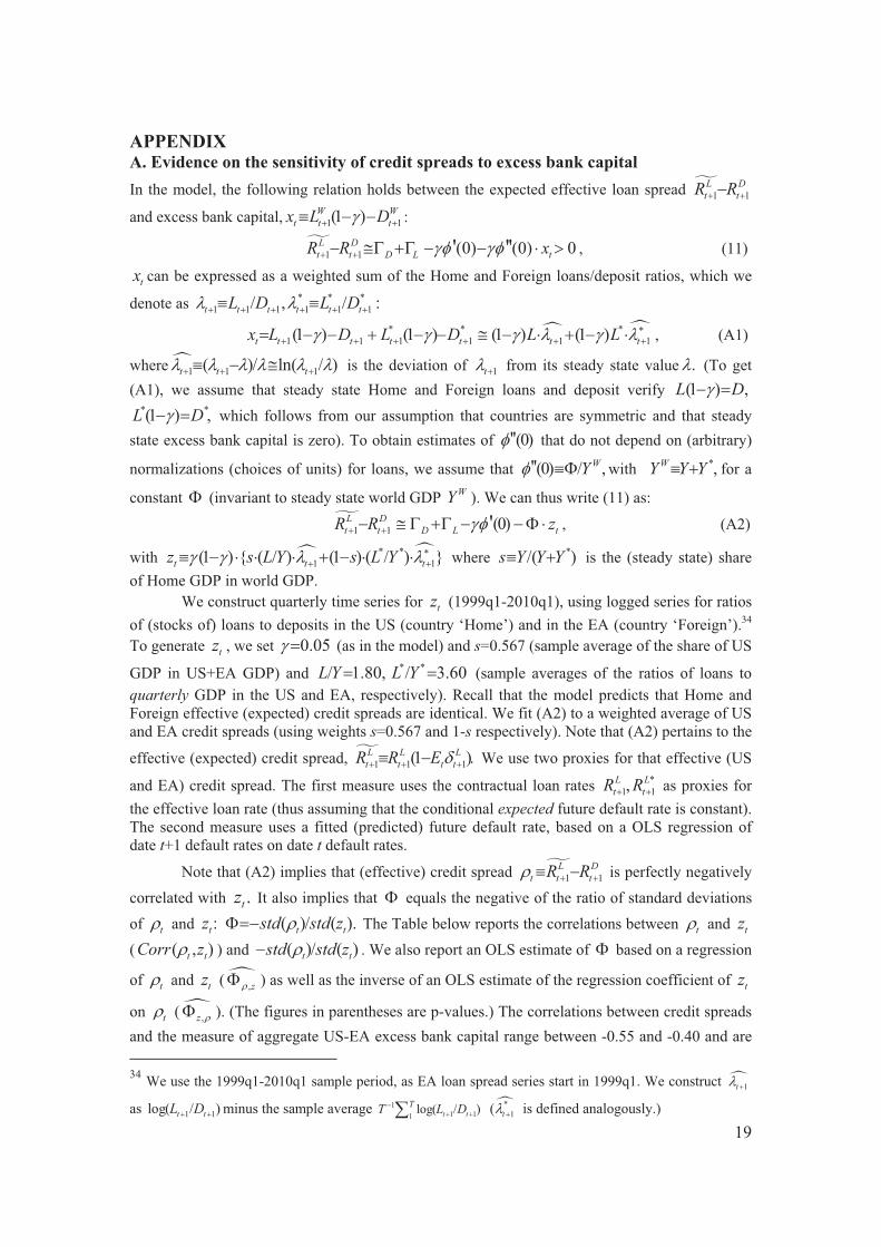
APPENDIX A. Evidence on the sensitivity of credit spreads to excess bank capital In the model, the following relation holds between the expected effective loan spread �1 1

L Dt tR R� ��

and excess bank capital, 1 1(1 )W Wt t tx L D�� �� � � :

�1 1 (0) (0) 0' ''L Dt t D L tR R x�� ��� �� �� �� � � � , (11)

tx can be expressed as a weighted sum of the Home and Foreign loans/deposit ratios, which we

denote as * * *1 1 1 1 1 1/ , / :t t t t t tL D L D� �� � � � � �� �

� �* * *1 1 1 1 1 1(1 ) (1 ) (1 ) (1 )t t t t t t tx L D L D L L� � � � � ��� � � � � �� � � � � � � � � � � � , (A1)

where�1 1 1( )/ ln( / )t t t� � � � � �� � �� � � is the deviation of 1t� � from its steady state value .� (To get (A1), we assume that steady state Home and Foreign loans and deposit verify (1 ) ,L D�� �

* *(1 ) ,L D�� � which follows from our assumption that countries are symmetric and that steady state excess bank capital is zero). To obtain estimates of (0)''� that do not depend on (arbitrary)

normalizations (choices of units) for loans, we assume that (0) / ,'' WY� �� with *,WY Y Y� � for a

constant � (invariant to steady state world GDP WY ). We can thus write (11) as:

�1 1 (0)'L Dt t D L tR R z��� �� � � �� � �� � , (A2)

with � �* *1 1(1 ) { ( / ) (1 ) ( / ) }t t tz s L Y s L Y� � � ��� �� � � � � � � � � where */( )s Y Y Y� � is the (steady state) share

of Home GDP in world GDP. We construct quarterly time series for tz (1999q1-2010q1), using logged series for ratios of (stocks of) loans to deposits in the US (country ‘Home’) and in the EA (country ‘Foreign’).34 To generate tz , we set 0.05� � (as in the model) and s=0.567 (sample average of the share of US

GDP in US+EA GDP) and / 1.80,L Y� * */ 3.60L Y � (sample averages of the ratios of loans to quarterly GDP in the US and EA, respectively). Recall that the model predicts that Home and Foreign effective (expected) credit spreads are identical. We fit (A2) to a weighted average of US and EA credit spreads (using weights s=0.567 and 1-s respectively). Note that (A2) pertains to the

effective (expected) credit spread, �1 1 1(1 ).L L Lt t t tR R E�� � �� � We use two proxies for that effective (US

and EA) credit spread. The first measure uses the contractual loan rates *1 1,L L

t tR R� � as proxies for the effective loan rate (thus assuming that the conditional expected future default rate is constant). The second measure uses a fitted (predicted) future default rate, based on a OLS regression of date t+1 default rates on date t default rates.

Note that (A2) implies that (effective) credit spread �1 1

L Dt t tR R� � �� � is perfectly negatively

correlated with .tz It also implies that � equals the negative of the ratio of standard deviations of t� and :tz ( )/ ( ).t tstd std z���� The Table below reports the correlations between t� and tz ( ( , )t tCorr z� ) and ( )/ ( )t tstd std z�� . We also report an OLS estimate of � based on a regression

of t� and tz (�,z�� ) as well as the inverse of an OLS estimate of the regression coefficient of tz

on t� (�,z �� ). (The figures in parentheses are p-values.) The correlations between credit spreads and the measure of aggregate US-EA excess bank capital range between -0.55 and -0.40 and are 34 We use the 1999q1-2010q1 sample period, as EA loan spread series start in 1999q1. We construct �1t� �

as 1 1log( / )t tL D� � minus the sample average 11 11

log( / )t tTT L D�

� � �*1( t� � is defined analogously.)

20

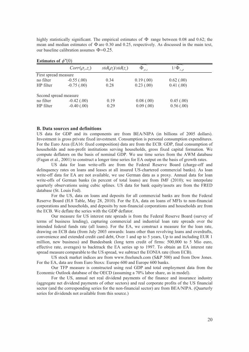
highly statistically significant. The empirical estimates of � range between 0.08 and 0.62; the mean and median estimates of � are 0.30 and 0.25, respectively. As discussed in the main text, our baseline calibration assumes 0.25.��

Estimates of ''(0)� ( , )t tCorr z� ( )/ ( )t tstd std z� �,z�� 1/�,z �� First spread measure no filter -0.55 (.00) 0.34 0.19 (.00) 0.62 (.00) HP filter -0.75 (.00) 0.28 0.23 (.00) 0.41 (.00) Second spread measure no filter -0.42 (.00) 0.19 0.08 (.00) 0.45 (.00) HP filter -0.40 (.00) 0.29 0.09 (.00) 0.56 (.00)

B. Data sources and definitions US data for GDP and its components are from BEA/NIPA (in billions of 2005 dollars). Investment is gross private fixed investment. Consumption is personal consumption expenditures. For the Euro Area (EA16: fixed composition) data are from the ECB: GDP, final consumption of households and non-profit institutions serving households, gross fixed capital formation. We compute deflators on the basis of nominal GDP. We use time series from the AWM database (Fagan et al., 2001) to construct a longer time series for EA output on the basis of growth rates. US data for loan write-offs are from the Federal Reserve Board (charge-off and delinquency rates on loans and leases at all insured US-chartered commercial banks). As loan write-off data for EA are not available, we use German data as a proxy. Annual data for loan write-offs of German banks (in percent of total loans) are from IMF (2010); we interpolate quarterly observations using cubic splines. US data for bank equity/assets are from the FRED database (St. Louis Fed). For the US, data on loans and deposits for all commercial banks are from the Federal Reserve Board (H.8 Table, May 28, 2010). For the EA, data on loans of MFIs to non-financial corporations and households, and deposits by non-financial corporations and households are from the ECB. We deflate the series with the GDP deflator. Our measure for US interest rate spreads is from the Federal Reserve Board (survey of terms of business lending), capturing commercial and industrial loan rate spreads over the intended federal funds rate (all loans). For the EA, we construct a measure for the loan rate, drawing on ECB data (from July 2003 onwards: loans other than revolving loans and overdrafts, convenience and extended credit card debt, Over 1 and up to 5 years, Up to and including EUR 1 million, new business) and Bundesbank (long term credit of firms: 500,000 to 5 Mio euro, effective rate, averages) to backtrack the EA series up to 1997. To obtain an EA interest rate spread measure comparable to the US spread, we subtract the EONIA rate (from ECB). US stock market indices are from www.freelunch.com (S&P 500) and from Dow Jones. For the EA, data are from Euro Stoxx: Europe 600 and Europe 600 banks. Our TFP measure is constructed using real GDP and total employment data from the Economic Outlook database of the OECD (assuming a 70% labor share, as in model). For the US, annual net real dividend payments of the finance and insurance industry (aggregate net dividend payments of other sectors) and real corporate profits of the US financial sector (and the corresponding series for the non-financial sector) are from BEA/NIPA. (Quarterly series for dividends not available from this source.)

21

References Acharya, V. and Schnabl, Ph. (2009). Do global banks spread global imbalances? The case of asset-backed commercial paper during the financial crisis of 2007–09, Working Paper, New York University. Aikman, D. and Paustian, M. (2006). Bank capital, asset prices and monetary policy. Working Paper 305, Bank of England. Ait-Sahalia, Y., Parker, J. and Yogo, M. (2004). Luxury goods and the equity premium. Journal of Finance, 56(6):2959–3004. Angeloni, I. and Faia, E. (2009). A Tale of two policies: prudential regulation and monetary policy with fragile banks. Working Paper, University of Frankfurt. Backus, D. K., Kehoe, P. J., and Kydland, F. E. (1992). International real business cycles. Journal of Political Economy, 100:745–775. BIS (2010). Statistical Annex, BIS Quarterly Review, Mach 2010, Bank for International Settlements. Brunnermeier, M. K. (2009). Deciphering the liquidity and credit crunch 2007-2008. Journal of Economic Perspectives, 23:77–100. Cetorelli, N. and Goldberg, L. S. (2008). Bank globalization, monetary transmission, and the lending channel, NBER Working Paper 14101. Cetorelli, N. and Goldberg, L. S. (2010). Global banks and international shock transmission: Evidence from the crisis. NBER Working Paper 15974. Christiano, L. and Eichenbaum, M. (1992). Current real business cycle theories and aggregate labor market fluctuations. American Economic Review, 82:430–450. Coeurdacier, N., Kollmann, R. and P. Martin (2010). International portfolios, capital accu- mulation and the dynamics of capital flows. Journal of International Economics, 80: 100-112. Correa, R., Sapriza, H. and A. Zlate (2010). International banks, the interbank market, and the cross-border transmission of business cycles. Working Paper, International Finance Section, Federal Reserve Board. Cúrdia, V. and M. Woodford (2009). Credit frictions and optimal monetary policy. Working Paper, NY Fed and Columbia University. Davis, S. (2010). The adverse feedback loop and the effects of risks in both the real and financial sectors. Working Paper 66, Globalization and Monetary Policy Institute, Federal Reserve Bank of Dallas. Dedola, L. and Lombardo, G. (2010). Financial frictions, financial integration and the international propagation of shocks. Working Paper, ECB. Devereux, M. B. and Yetman, J. (2010). Leverage constraints and the international transmission of shocks. Journal of Money, Credit and Banking, 42: 71-105. de Walque, G., Pierrard, O. and Rouabah, A. (2009). Financial (in)stability, supervision and liquidity injections: A dynamic general equilibrium approach. Economic Journal, forthcoming. Dewatripont, M. and Tirole, J. (1994). The Prudential Regulation of Banks. MIT Press. D’Hulster, K. (2009). The leverage ratio. Memo, World Bank-IFC. Dib, A. (2010). Banks, credit market frictions, and business cycles. Bank of Canada. ECB (2010). Financial stability review (June 2010), European Central Bank. Fagan, G., Henry, J., and Mestre, R. (2001). An area-wide model (AWM) for the euro area. ECB Working Paper 42. Freixas, X. and Rochet, J.-C. (2008). Microeconomics of Banking. Cambridge: The MIT Press. Gerali, A., Neri, S., Sessa, L., and Signoretti, F. M. (2010). Credit and banking in a DSGE model of the Euro Area. Journal of Money, Credit, and Banking 42 (issue supplement S1), 107-141. Gertler, M. and Kiyotaki, N. (2010). Financial intermediation and credit policy in business cycle analysis. Working Paper, New York University. Giannone, D., Lenza, M., and Reichlin, L. (2010). Euro area and US recessions. ECB Working Paper. Goodfriend, M. and McCallum, B. T. (2007). Banking and interest rates in monetary policy analysis: A quantitative exploration. Journal of Monetary Economics, 54:1480–1507.

22

Hubbard, G., Kuttner, K. and Palia, D. (2002). Are there bank effects in borrowers’ costs of funds? Evidence from a matched sample of borrowers and banks. Journal of Business, 75: 559-580. Huizinga, H. and Laeven, L. (2009). Accounting discretion and banks during a financial crisis. Working Paper, Tilburg University and IMF. Iacoviello, M. (2010). Financial business cycles. Working Paper, Boston College. IMF (2010). Global financial stability report (April 2010), International Monetary Fund. King, R. G. and Rebelo, S. T. (1999). Resuscitating real business cycles. Handbook of Macroeconomics, Volume 1, pp. 927 – 1007. Elsevier. Kiyotaki, N. and Moore, J. (1997). Credit cycles. Journal of Political Economy, 105:211– 248. Kiyotaki, N. and Moore, J. (2005). Liquidity and asset prices. International Economic Review, 46(2):317–349. Kollmann, R. (1996). Incomplete asset markets and the cross-country consumption correlation puzzle. Journal of Economic Dynamics and Control, 20(5):945 – 961. Kollmann, R (2010). Banks and the Domestic and International Propagation of Macroeconomic and Financial Shocks, Working Paper. Presented at May 2010 Konstanz Seminar on Monetary Theory and Policy. Krugman, P. and Obstfeld, M. (2008). International economics: Theory and policy (8th edition), Pearson International. Meh, C. A. and Moran, K. (2010). The role of bank capital in the propagation of shocks. Journal of Economic Dynamics and Control, 34:555–576. Mendoza, E. G. and Quadrini, V. (2010). Financial globalization, financial crisis and contagion. Journal of Monetary Economics, 57:24–39. Obstfeld, M. and Rogoff, K. (1996). Foundations of International Macroeconomics. MIT Press. Olivero, M. P. (2010). Market power in banking, countercyclical margins and the international transmission of business cycles. Journal of International Economics, 80:292–301. Parker, J. and Vissing-Jorgensen, A. (2009). Who bears aggregate fluctuations and how? American Economic Review, 99(2):399–405. Perri, F. and Quadrini, V. (2010). International recessions. Working Paper, USC. Puri, M., Rocholl, J., and Steffen, S. (2010). Global retail lending in the aftermath of the US financial crisis: Distinguishing between supply and demand effects. Journal of Financial Economics, forthcoming. Roeger, W. (2009). The financial crisis 2008 in the QUEST model: Impact on Europe. Working Paper, DG ECFIN, EU Commission. Santos, J. and Winton, A. (2009). Bank Capital, Borrower Power, and Loan Rates. Working Paper, NY Fed and University of Minnesota. Ueda, K. (2010). Banking globalization and international business cycles. Working Paper, Institute for Monetary and Economic Studies, Bank of Japan. Van den Heuvel, S. J. (2008). The welfare cost of bank capital requirements. Journal of Monetary Economics, 55: 298–320. von Peter, G. (2009). Asset prices and banking distress: a macroeconomic approach. Journal of Financial Stability, 5: 298-319.

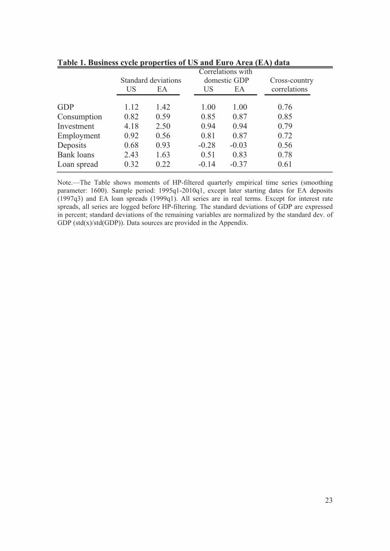
23

Table 1. Business cycle properties of US and Euro Area (EA) data Correlations with Standard deviations domestic GDP Cross-country US EA US EA correlations GDP 1.12 1.42 1.00 1.00 0.76 Consumption 0.82 0.59 0.85 0.87 0.85 Investment 4.18 2.50 0.94 0.94 0.79 Employment 0.92 0.56 0.81 0.87 0.72 Deposits 0.68 0.93 -0.28 -0.03 0.56 Bank loans 2.43 1.63 0.51 0.83 0.78 Loan spread 0.32 0.22 -0.14 -0.37 0.61 Note.—The Table shows moments of HP-filtered quarterly empirical time series (smoothing parameter: 1600). Sample period: 1995q1-2010q1, except later starting dates for EA deposits (1997q3) and EA loan spreads (1999q1). All series are in real terms. Except for interest rate spreads, all series are logged before HP-filtering. The standard deviations of GDP are expressed in percent; standard deviations of the remaining variables are normalized by the standard dev. of GDP (std(x)/std(GDP)). Data sources are provided in the Appendix.

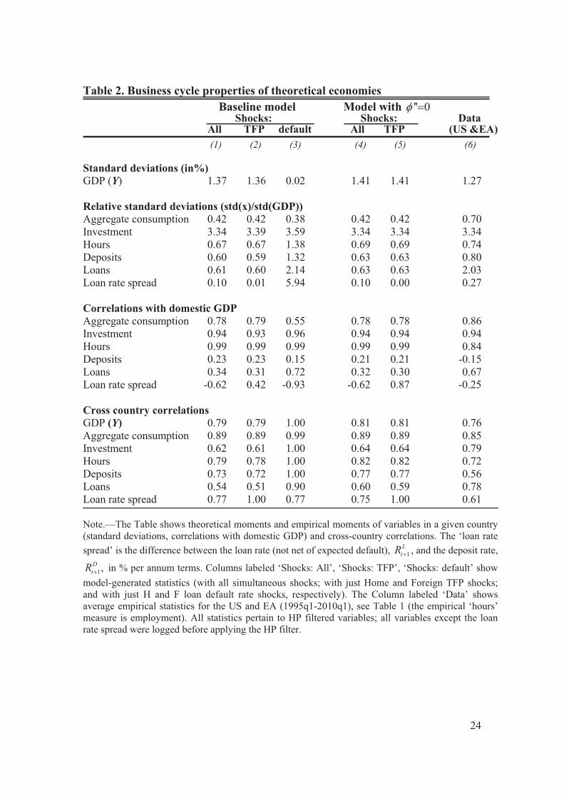
24

Table 2. Business cycle properties of theoretical economies Baseline model Model with '' 0� � Shocks: Shocks: Data All TFP default All TFP (US &EA) (1) (2) (3) (4) (5) (6)

Standard deviations (in%) GDP (Y) 1.37 1.36 0.02 1.41 1.41 1.27 Relative standard deviations (std(x)/std(GDP)) Aggregate consumption 0.42 0.42 0.38 0.42 0.42 0.70 Investment 3.34 3.39 3.59 3.34 3.34 3.34 Hours 0.67 0.67 1.38 0.69 0.69 0.74 Deposits 0.60 0.59 1.32 0.63 0.63 0.80 Loans 0.61 0.60 2.14 0.63 0.63 2.03 Loan rate spread 0.10 0.01 5.94 0.10 0.00 0.27 Correlations with domestic GDP Aggregate consumption 0.78 0.79 0.55 0.78 0.78 0.86 Investment 0.94 0.93 0.96 0.94 0.94 0.94 Hours 0.99 0.99 0.99 0.99 0.99 0.84 Deposits 0.23 0.23 0.15 0.21 0.21 -0.15 Loans 0.34 0.31 0.72 0.32 0.30 0.67 Loan rate spread -0.62 0.42 -0.93 -0.62 0.87 -0.25 Cross country correlations GDP (Y) 0.79 0.79 1.00 0.81 0.81 0.76 Aggregate consumption 0.89 0.89 0.99 0.89 0.89 0.85 Investment 0.62 0.61 1.00 0.64 0.64 0.79 Hours 0.79 0.78 1.00 0.82 0.82 0.72 Deposits 0.73 0.72 1.00 0.77 0.77 0.56 Loans 0.54 0.51 0.90 0.60 0.59 0.78 Loan rate spread 0.77 1.00 0.77 0.75 1.00 0.61 Note.—The Table shows theoretical moments and empirical moments of variables in a given country (standard deviations, correlations with domestic GDP) and cross-country correlations. The ‘loan rate spread’ is the difference between the loan rate (not net of expected default), 1

LtR � , and the deposit rate,

1,DtR � in % per annum terms. Columns labeled ‘Shocks: All’, ‘Shocks: TFP’, ‘Shocks: default’ show

model-generated statistics (with all simultaneous shocks; with just Home and Foreign TFP shocks; and with just H and F loan default rate shocks, respectively). The Column labeled ‘Data’ shows average empirical statistics for the US and EA (1995q1-2010q1), see Table 1 (the empirical ‘hours’ measure is employment). All statistics pertain to HP filtered variables; all variables except the loan rate spread were logged before applying the HP filter.

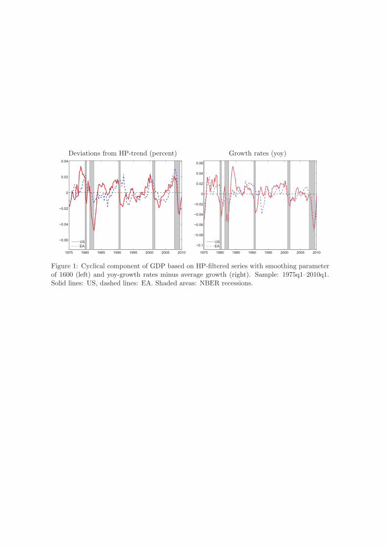
Deviations from HP-trend (percent) Growth rates (yoy)

1975 1980 1985 1990 1995 2000 2005 2010

−0.06

−0.04

−0.02

0

0.02

0.04

USEA

1975 1980 1985 1990 1995 2000 2005 2010

−0.1

−0.08

−0.06

−0.04

−0.02

0

0.02

0.04

0.06

USEA

Figure 1: Cyclical component of GDP based on HP-filtered series with smoothing parameterof 1600 (left) and yoy-growth rates minus average growth (right). Sample: 1975q1–2010q1.Solid lines: US, dashed lines: EA. Shaded areas: NBER recessions.

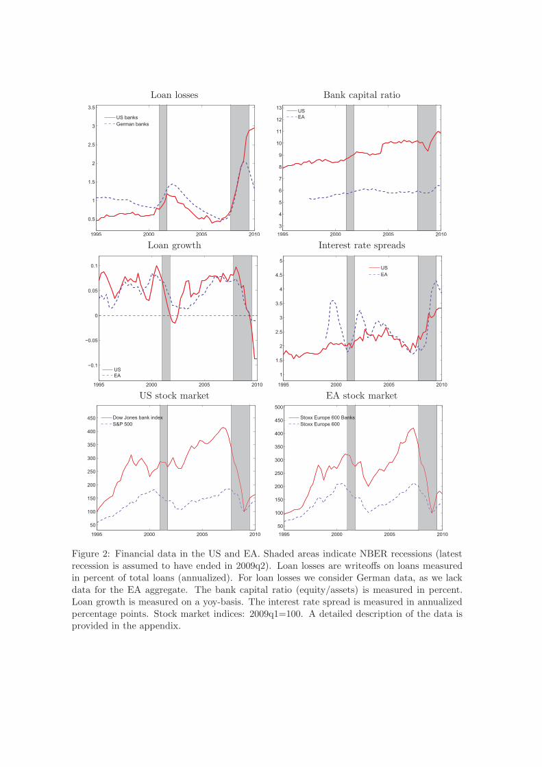
Loan losses Bank capital ratio

1995 2000 2005 2010

0.5

1

1.5

2

2.5

3

3.5

US banksGerman banks

1995 2000 2005 20103

4

5

6

7

8

9

10

11

12

13 USEA

Loan growth Interest rate spreads

1995 2000 2005 2010

−0.1

−0.05

0

0.05

0.1

USEA

1995 2000 2005 2010

1

1.5

2

2.5

3

3.5

4

4.5

5USEA

US stock market EA stock market

1995 2000 2005 2010

50

100

150

200

250

300

350

400

450 Dow Jones bank indexS&P 500

1995 2000 2005 201050

100

150

200

250

300

350

400

450

500

Stoxx Europe 600 BanksStoxx Europe 600

Figure 2: Financial data in the US and EA. Shaded areas indicate NBER recessions (latestrecession is assumed to have ended in 2009q2). Loan losses are writeoffs on loans measuredin percent of total loans (annualized). For loan losses we consider German data, as we lackdata for the EA aggregate. The bank capital ratio (equity/assets) is measured in percent.Loan growth is measured on a yoy-basis. The interest rate spread is measured in annualizedpercentage points. Stock market indices: 2009q1=100. A detailed description of the data isprovided in the appendix.

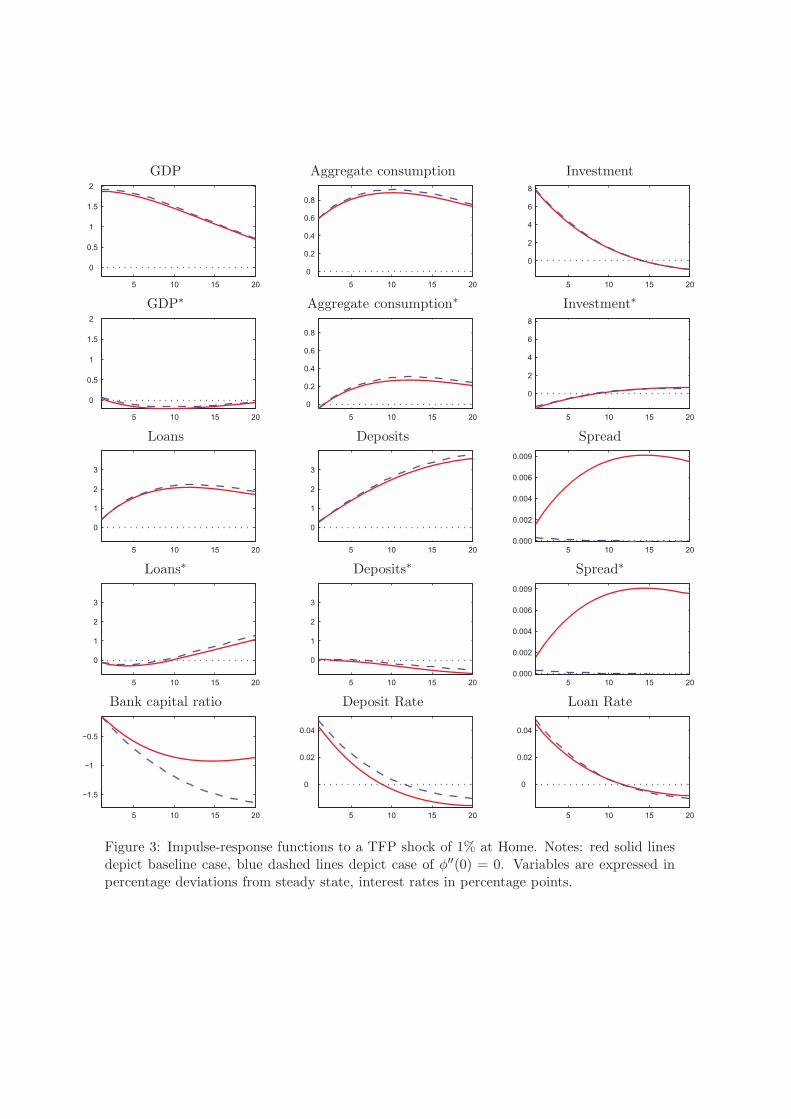
GDP Aggregate consumption Investment

5 10 15 20

0

0.5

1

1.5

2

5 10 15 200

0.2

0.4

0.6

0.8

5 10 15 20

0

2

4

6

8

GDP∗ Aggregate consumption∗ Investment∗

5 10 15 20

0

0.5

1

1.5

2

5 10 15 200

0.2

0.4

0.6

0.8

5 10 15 20

0

2

4

6

8

Loans Deposits Spread

5 10 15 20

0

1

2

3

5 10 15 20

0

1

2

3

5 10 15 200.000

0.002

0.004

0.006

0.009

Loans∗ Deposits∗ Spread∗

5 10 15 20

0

1

2

3

5 10 15 20

0

1

2

3

5 10 15 200.000

0.002

0.004

0.006

0.009

Bank capital ratio Deposit Rate Loan Rate

5 10 15 20

−1.5

−1

−0.5

5 10 15 20

0

0.02

0.04

5 10 15 20

0

0.02

0.04

Figure 3: Impulse-response functions to a TFP shock of 1% at Home. Notes: red solid linesdepict baseline case, blue dashed lines depict case of φ′′(0) = 0. Variables are expressed inpercentage deviations from steady state, interest rates in percentage points.

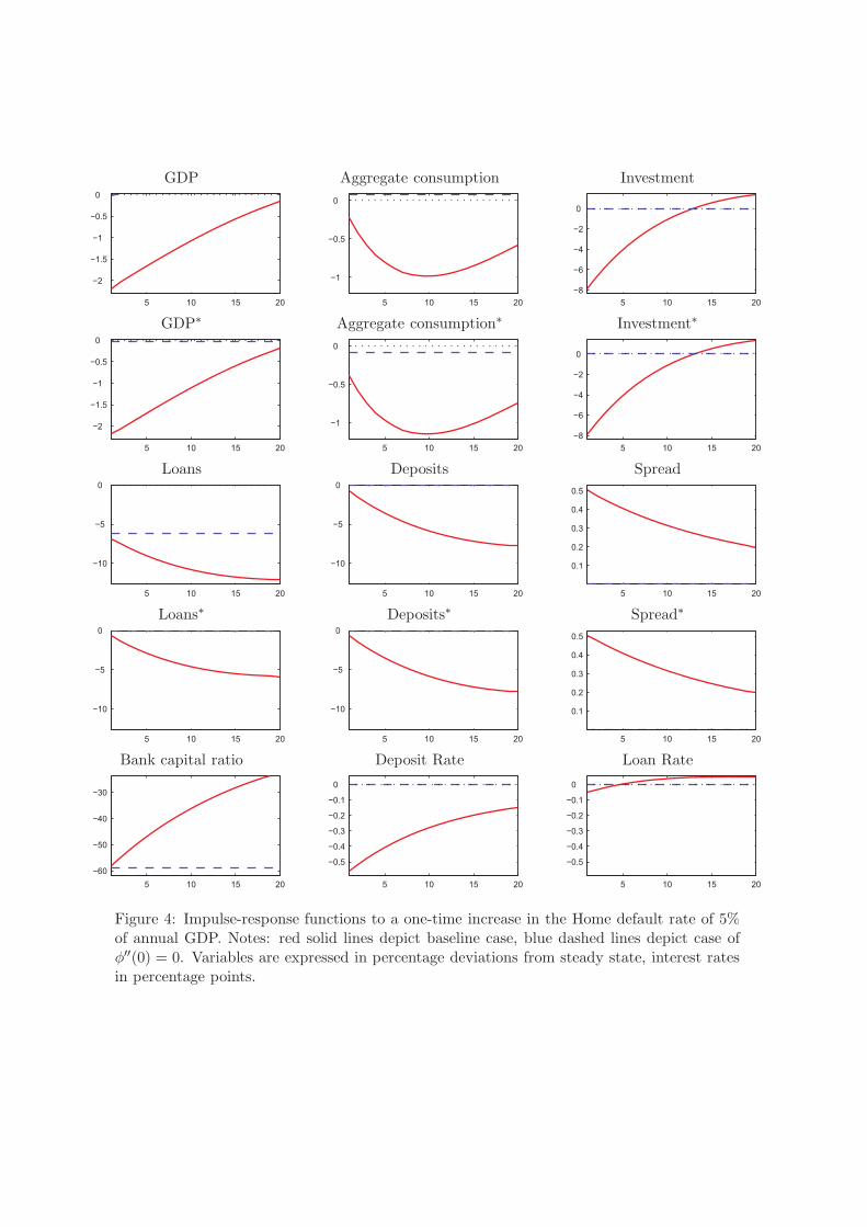
GDP Aggregate consumption Investment

5 10 15 20

−2

−1.5

−1

−0.5

0

5 10 15 20

−1

−0.5

0

5 10 15 20−8

−6

−4

−2

0

GDP∗ Aggregate consumption∗ Investment∗

5 10 15 20

−2

−1.5

−1

−0.5

0

5 10 15 20

−1

−0.5

0

5 10 15 20−8

−6

−4

−2

0

Loans Deposits Spread

5 10 15 20

−10

−5

0

5 10 15 20

−10

−5

0

5 10 15 20

0.1

0.2

0.3

0.4

0.5

Loans∗ Deposits∗ Spread∗

5 10 15 20

−10

−5

0

5 10 15 20

−10

−5

0

5 10 15 20

0.1

0.2

0.3

0.4

0.5

Bank capital ratio Deposit Rate Loan Rate

5 10 15 20−60

−50

−40

−30

5 10 15 20

−0.5

−0.4

−0.3

−0.2

−0.1

0

5 10 15 20

−0.5

−0.4

−0.3

−0.2

−0.1

0

Figure 4: Impulse-response functions to a one-time increase in the Home default rate of 5%of annual GDP. Notes: red solid lines depict baseline case, blue dashed lines depict case ofφ′′(0) = 0. Variables are expressed in percentage deviations from steady state, interest ratesin percentage points.

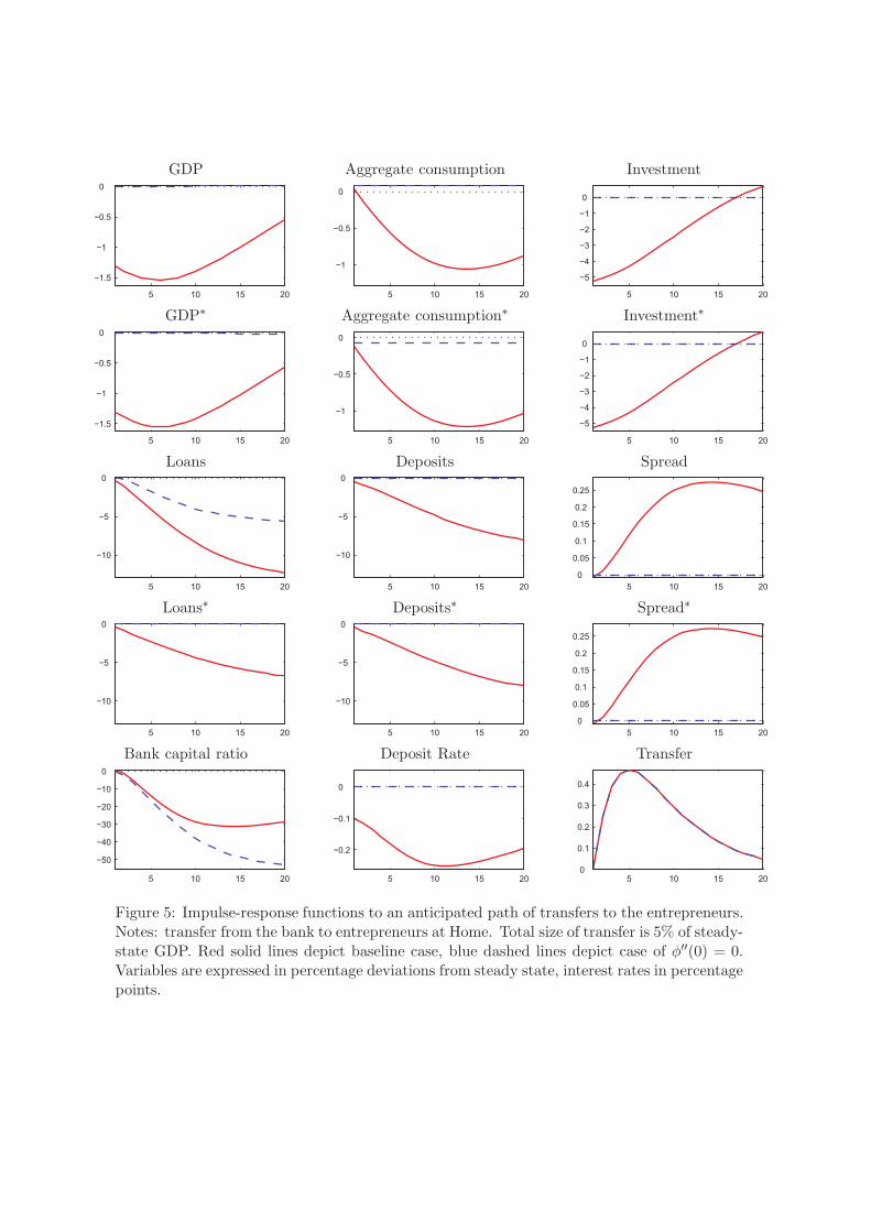
GDP Aggregate consumption Investment

5 10 15 20

−1.5

−1

−0.5

0

5 10 15 20

−1

−0.5

0

5 10 15 20

−5

−4

−3

−2

−1

0

GDP∗ Aggregate consumption∗ Investment∗

5 10 15 20

−1.5

−1

−0.5

0

5 10 15 20

−1

−0.5

0

5 10 15 20

−5

−4

−3

−2

−1

0

Loans Deposits Spread

5 10 15 20

−10

−5

0

5 10 15 20

−10

−5

0

5 10 15 200

0.05

0.1

0.15

0.2

0.25

Loans∗ Deposits∗ Spread∗

5 10 15 20

−10

−5

0

5 10 15 20

−10

−5

0

5 10 15 200

0.05

0.1

0.15

0.2

0.25

Bank capital ratio Deposit Rate Transfer

5 10 15 20

−50

−40

−30

−20

−10

0

5 10 15 20

−0.2

−0.1

0

5 10 15 200

0.1

0.2

0.3

0.4

Figure 5: Impulse-response functions to an anticipated path of transfers to the entrepreneurs.Notes: transfer from the bank to entrepreneurs at Home. Total size of transfer is 5% of steady-state GDP. Red solid lines depict baseline case, blue dashed lines depict case of φ′′(0) = 0.Variables are expressed in percentage deviations from steady state, interest rates in percentagepoints.

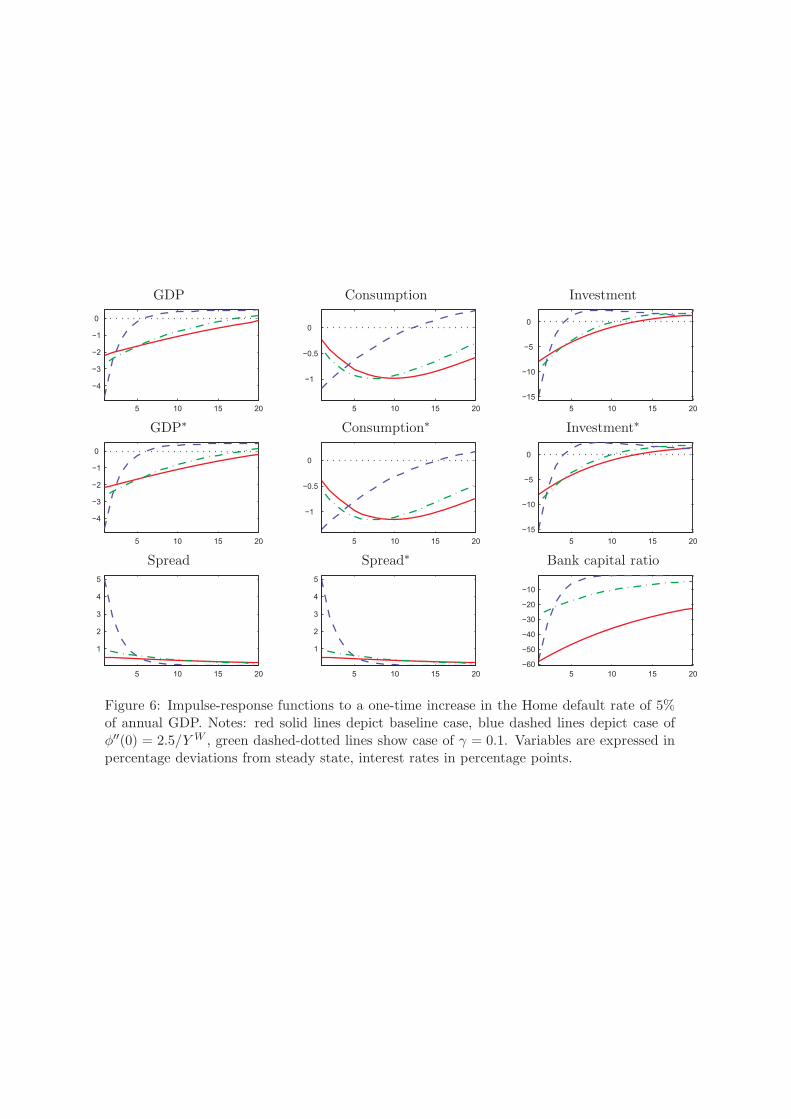
GDP Consumption Investment

5 10 15 20

−4

−3

−2

−1

0

5 10 15 20

−1

−0.5

0

5 10 15 20−15

−10

−5

0

GDP∗ Consumption∗ Investment∗

5 10 15 20

−4

−3

−2

−1

0

5 10 15 20

−1

−0.5

0

5 10 15 20−15

−10

−5

0

Spread Spread∗ Bank capital ratio

5 10 15 20

1

2

3

4

5

5 10 15 20

1

2

3

4

5

5 10 15 20−60

−50

−40

−30

−20

−10

Figure 6: Impulse-response functions to a one-time increase in the Home default rate of 5%of annual GDP. Notes: red solid lines depict baseline case, blue dashed lines depict case ofφ′′(0) = 2.5/Y W , green dashed-dotted lines show case of γ = 0.1. Variables are expressed inpercentage deviations from steady state, interest rates in percentage points.