Global Changes in Postglacial Sea Level: A Numerical

QUATERNARY RESEARCH 9, 265-281 (1978)

Global Changes in Postglacial Sea Level: A Numerical Calculation1

JAMES A. CLARK

Department of Geological Sciences, Cornell Universiiy, Ithaca, N. Y. I4853

WILLIAM E. FARRELL

Department of Engineering Geoscience, University of California. Berkeley, Cal$ 94720

AND

W. RICHARD PELTIER

Department of Physics, University of Toronto, Toronto, Ontario MjS-IA7, Canada

Received June 28, 1977

The sea-level rise due to ice-sheet melting since the last glacial maximum was not uniform everywhere because of the deformation of the Earth’s surface and its geoid by changing ice and water loads. A numerical model is employed to calculate global changes in relative sea level on a spherical viscoelastic Earth as northern hemisphere ice sheets melt and fill the ocean basins with meltwater. Predictions for-the paw explain a large proportion of the global variance in the sea-level record, particularly during the Halacene. Results indicate that the oceans can be divided into six zones, each of which is characterized by a specific form of the relative sea-level curve. In four of these zones emerged beaches are predicted, and these may form even at considerable distance from the ice sheets themselves. In the remaining zones submergence is dominant, and no emerged beaches are expected. The close agreement of these predictions with the data suggests that, contrary to the beliefs of many, no net change in ocean volume has occurred during the past 5000 years. Predictions for localities close to the ice sheets are the most in error, suggesting that slight modifications of the assumed melting history and/or the rheological model of the Earth’s interior are necessary.

INTRODUCTION

Relict shoreline features of Holocene age well below the present sea level (e.g., Fair- bridge, 1961; Shepard, 1963; Emery and Garrison, 1967; Bloom, 1970) strongly support the belief that as the ice sheets retreated following the last glacial maximum their meltwater increased the volume of the oceans. However, not all submerged indicators of shorelines of the same age lie at the same elevation, indicating that the ocean did not rise uniformly relative to the land. It has often been suggested that, because the Earth is not rigid, this nonuniform rise of reiative sea level would be expected even at large distances from

1 Contribution number 614 of Cornell University Department of Geological Sciences.

the melting ice (Daly, 1934; Wellman, 1964; Bloom, 1967; Walcott, 1972a; Chappell, 1974; Cathles, 1975; Peltier and Andrews, 1976). Walcott (1972a), in particular, considered the global distribution of relative sea level during the past 20,000 years. He, among others, showed that because the reduced ice load caused gravitational (isostatic) disequilibrium, the land in regions once glaciated should rise relative to the sea surface. Peripheral to the glacial margin, submergence is expected because material from this region is depleted when Earth material flows into the uplifting region. Walcott’s major contribution, however, was to show how relative sea level at great distances from the glaciated regions is affected by meltwater loading of the

265 0033-5894/78/0093-0265$02.00/O Copyright 8 I!278 by the University of Washington. AU rights of reproduction in any form reserved.

266 CLARK, FARRELL AND PELTIER

ocean floor. Assuming that the effect of glacial unloading is negligible at great distances from the ice, Walcott found that the continents should rise slightly relative to the ocean floor. Walcott used viscous flat Earth models and decoupled the glacial- unloading problem from the water-loading problem. Cathles (1975) improved upon Walcott’s approach by using a more realistic spherical viscoelastic Earth model. He allowed both glacial melting and the asso- ciated ocean filling to distort the solid surface of the Earth through time. His con- clusions support those of Walcott. Chappell (1974) considered a viscous flat Earth, but the sloping continental shelf in his model allowed the ocean to advance inland as the ocean basins filled. Peltier and Andrews (1976) used a different and more-exact approach to do an analysis similar to that

ICE

Load /\

Moss Attraction

Attraction

G

FIG. 1. Interactions among ice loads, water loads, and the deformable Earth: (A) The weight of the ice deforms the Earth and (B) the ice mass attracts the water. (C) The transfer of matter within the Earth distorts the geoid. Similarly, (D) the weight of meltwater depresses the Earth differentially and (E) more water flows into this depression, increasing the water load and (F) causing added deformation of the ocean floor. These processes are interrelated as indicated in (G), and all are included in the numerical model.

of Cathles (1975). All of these methods have a common fault, they consider only the distortion of the solid surface of the Earth. In reality, the observed change in relative sea level is the change in distance between the ocean floor and the ocean surface. The surface of the equilibrium ocean is always at constant gravitational potential, and this surface defines the geoid. As ice melts on the surface of the Earth and matter within the Earth flows to com- pensate for the changing surface-mass distribution, the combined mass transfers affect the geoid. Farrell and Clark (1976) and Clark (1976) have shown that these changes of the geoid can be of the same order of magnitude as the oceanwide average rise in sea level (commonly known as the eustatic rise) resulting from t‘Ae meltwater increase of the ocean volume.

To calculate relative sea level, therefore, the changes in separation between two dynamic surfaces-the ocean floor and the ocean surface-must be determined. To do this properly requires consid- eration of the interactions schematically represented in Fig. 1 and described in the figure caption. These processes are inex- tricably related because the water load is a function of both the changing ice load and the changing distance between the ocean floor and the geoid (Fig. 1G). For a spherical viscoelastic Earth with realistic ocean configurations and glacial history, Farrell and Clark (1976) showed how to calculate the relative sea-level change at any location when the interactions of Fig. 1 are considered. Results of this “self-consistent” calculation of the history of the global sea level for a likely glacial history and Earth rheology are given below.

THE MODEL

The Earth behaves as an elastic material for applied stresses of short time scale (earthquakes) and as a fluid for stresses of long duration (centrifugal force), but

GLOBAL POSTGLACIAL SEA LEVEL 267

the 20,000-year time span for stresses in- volving glacial melting and Earth relaxation is of intermediate duration. Both elastic and viscous behavior will, therefore, be important. A Maxwell viscoelastic material is thus a plausible rheological model for the problem considered here, and it has been employed previously (Cathles, 1975; Pel- tier and Andrews, 1976). The behavior of this material is analogous to an elastic spring in series with a viscous dashpot. A stress applied to such an element causes immediate distortion of the spring but slow time-dependent distortion of the dashpot. In this study, the Earth model is a spherically symmetric self-gravitating Maxwell material. The elastic properties and density vary with depth like those of a Gutenberg- Bulien elastic Earth model A (e.g., Alter- man et ul., 1961) determined by seismic methods. The anelasticity of the model is determined by a single parameter, the New- tonian viscosity V; we assume v to be 1V2 P (cgs.) throughout the Earth’s mantle and 0 P in the Earth’s core. The rheology of the real Earth may differ substantially from that of a Maxwell material. In particular, the relation between applied stress and strain rate may be nonlinear, which is to say that the material is not Newtonian. The philosophy which we adopt here is that the simple linear model should be subjected to direct test before it is rejected. Peltier (1974) discussed these matters in greater detail.

The areal extent of the ice is approxi- mated on a 5” latitude x 5” longitude grid, and the ice thickness on each grid element is varied independently at IOOO-year intervals. Two glacial histories are considered and will be discussed in detail below. We also assume that isostatic compensation is complete by the time the ice sheets begin to disintegrate.

The method for calculating relative sea level has been described previously by Farrell and Clark (1976) and is reviewed only briefly here. For any spherically symmetric viscoelastic Earth model the

time-dependent change in separation between the Earth’s surface and the geoid caused by a point load placed on the Earth’s surface can be calculated (Peltier, 1974). This function is called a viscoelastic Green function (Peltier, 1974). In order to determine the effect of a load with a realistic spatial distribution, the load is considered to be a collection of point loads, and the effects are added. Similarly, if the load is time dependent, the effects of all past loads are added to the effects of the present loads. Farrell and Clark (1976) showed that the explicit expression for sea-level change s at time t and position vector r is

s(t,r) = il

GE(r - r ‘)pg(t,r ‘)dW OCean

+ G”(r - r’)pJ(f,r’)diY Ice

G”(r - 7, r - r’)

x [pws(T,r’) + pJ(r,r’)]dS2’

where:

GE is the immediate-response elastic Green function,

GV is the time-dependent viscous Green function,

pw is the density of water, px is the density of ice, Z is the ice thickness, da’ is an element of area, kE corrects for the oceanwide average rise

in sea level (eustatic rise), k, insures that mass is conserved, and the notation r -r ’ indicates the angu-

lar distance between position vectors r and r’.

The third term in Eq. (1) represents the slow deformation of the Earth from changes in both ice and water loads. The second term accounts for the immediate elastic sea-level response due to the change in ice load. The first term is


FIG. 2. A schematic illustration of the Heaviside Green function. The distortion of a reference shoreline 1000, 5000, and 15,000 years after the melting of a point ice mass is illustrated in (A). Five distinct spatially dependent sea-level regions are given on the distance axis, which is only approximate. The sea-level change relative to the initial reference shoreline at selected locations in (A) is given in (B). Each region has a distinctly different expression in the sea-level record. In Region 1, for example, the land rises continuously relative to the sea (a); whereas in Region V, sea level rises rapidly initially, but this submergence is followed by slow emergence (g).

the immediate sea-level change caused by changes in water load. The sea-level solution s is also found under the integral on the right side of Eq. (l), making this an integral equation. The integral equation results because the changing sea level causes a corresponding variation in the water load. This feedback effect described by Eq. (l), ‘therefore, accounts for all of the interactions illustrated in Fig. 1. The integral equation can be solved numerically with an iterative scheme that ensures the conservation of mass. Equation (1) con- verges rapidly upon a solution for sea level, and sea-level results can be compared directly to observed relative sea-level curves. No correction for eustatic rise in

sea level is necessary. Hence for a given Earth rheology and glacial history, it is possible to calculate time-dependent relative sea-level changes for any location. A very stringent test of the assumed Earth model and glacial history is therefore possible, because for the model to succeed it must fit data from (1) the ocean centers, (2) the continental margins, (3) the fore- buige region, and (4) the glaciated regions.

THE SEA-LEVEL GREEN FUNCTION

Equation (1) indicates that the viscoelastic Green function is crucial in deter- mining worldwide sea-level changes. The form of the time-dependent Green function,


therefore, gives usefti4 insight into the expected global sea-level response. Because of the utility of the ,concept, the Green function that results from a point load remaining on the Earth’s surface is now briefly considered. This Heaviside Green function was calculated by Peltier (Peltier, 1974; Peltier and Andrews, 1976). It is the simplest treatment of the sea-level problem pre- sented in this study because the ice sheets are assumed to be collected into a point and all ocean-loading effects are ignored. To ensure clarity, we begin by considering a schematic illustration of the relative sea- level change at three different times (1000, 5000, and 15,000 years) after removal of the point ice load (Fig. 2). The actual Heavi- side Green function used here was given by Peltier and Andrews (1976), and Fig. 2 illustrates only its viscous part. It varies over several orders of magnitude and is difficult to interpret graphically, but Fig. 2 contains all of the essential information in the Green function needed to interpret relative sea-level expression through time. The horizontal axis gives the approximate distance scale, while the vertical axis represents relative sea-level change. Because of the unrealistic assumptions, only the shapes of these curves are considered relative to the original sea-level configuration. Actual amounts of sea-level change are more ap- propriately considered in subsequent sections, where realistic ocean and ice configurations and all of the processes illustrated in Fig. 1 are included.

Figure 2 is divided into five regions, each of which is characterized by a sea-level signature unique to that region. In Region-I the land rises continuously, relative to sea level, through the 15,000-year time interval. The rate of this emergence decreases through time. The total amount of emergence in Region I is a function of position, with greater emergence occurring closer to the point load.

In Region II there is a continual submergence due to the presence of the collapsing proglacial forebulge, and the relative degree

of submergence is again a function of position. For this viscosity model, the forebulge does not collapse in place, rather it “mi- grates” toward the ice load as it collapses (Peltier, 1974; Cothles, 1975). This migration produces a domain of transition between Regions I and II characterized by initial emergence followed later in time by a falling of the land relative to the sea surface (submergence). Depending upon position with respect to the load, these relative motions result in either more emergence than submergence or more submergence than emergence. with greater submergence occurring at greater distances from the ice. Because of the migration of the collapsing forebulge, the time when the land stops rising relative to the sea and begins to submerge is dependent upon position. Submergence will com- mence at a later time for sites close to the ice than for sites at greater distances.

In Region III the trend of relative sea- level change is just the opposite of the trend in the Transition Region. In Region III the land first sinks relative to the ocean’s surface and then emerges slightly. These relative motions are also due to the time-dependent shape of the migrating forebulge, and again the time of maximum submergence is a function of location.

In Region IV there is continual submergence, but of lesser magnitude than in Region II. At a great distance from the ice (Region V), the relative sea-level curve is not monotonic. Initial submergence is followed by slight emergence, but this emergence is much smaller in magnitude than the emergence in Region I.

The above discussion emphasizes the importance of the concept of the migrating forebulge and illustrates the approximate expression of it which should be evident in the sea-level record. The time-dependent configuration of the forebulge is a function of the viscosity profile, which may differ from the assumed profile of this model. Peltier (1974) has shown that if the lower mantle has a very high viscosity (10z4 P), the forebulge will not migrate as it collapses.


FIG. 3. Realistic distribution of glacial ice. A uniform 1000 m of ice was melted instantaneously at 18,000 B.P. from all of these glaciated regions. The immediate eustatic rise in sea level was then 77.5 m.

For an Earth model with a low-viscosity aesthenosphere (102l P), the amplitude of the migrating forebulge will increase substantially. The viscosity profile used here is thus a compromise between these two possible viscosity profiles, and Peltier (1976) has described a method whereby the most likely profile may be determined.

UNIFORM INSTANTANEOUS ICE MELTING

In the previous discussion, the analysis of the Green function delineated the characteristic sea level response for five regions on a viscoelastic Earth model with uniform viscosity. Next, a more realistic case is considered, in which ocean loading and all of the interactions of Fig. 1 are included. Furthermore, the ice sheets have the realistic spatial configuration illustrated in Fig. 3. The assumed glacial history is a simple one in which a uniform 1000 m of ice melt instantaneously (at 18,000 B.P.) from all glaciated regions of Fig. 3. The eustatic rise is then a step function in time with an amplitude of 77.5 m. Although the ice melts at one instant (18,000 B.P.), Fig. 4 indicates that the relative sea level con- tinues to change during the following 10,000

years as the Earth relaxes. The North Atlan- tic Ocean becomes deeper in contrast to the shallowing of the South Pacific. In regions under the ice, the relative sea level falls more rapidly than the oceans fill, resulting in emerged beaches.’ Similarly, in the South Pacific relative sea level rises while meltwater flows into the oceans, but when melting stops, sea level falls.

Emerged beaches are easily observed and frequently dated, whereas submerged beaches are more difficult to identify and to date. However, there is at present considerable controversy over the significance and cause of emerged Holocene beaches found in regions far from glaciated areas. Some claim that these beaches were formed by a postglacial eustatic sea level higher than present and thereby infer important climatic changes (e.g., Schofield, 1964; Gill, 1965; Fairbridge, 1976). Others disa- gree with this contention and suggest that the numerous emerged beaches are either

I Here, as in the remaining sections, we use the term “beach” rather loosely to include an entire assemblage of shore-zone landforms and sediments which are indicators of the position of local sea level. This assemblage includes such features as beaches, shore erosional platforms, reefs, deltas, coastal dune ridges, and salt-water marshes.


FIG. 4. Percentage of eustatic sea-level change predicted by the viscoelastic sea-level model with uniform instantaneous ice melting. At 18,000 B.P. a uniform amount of ice was melted from all Late Wisconsin ice sheets shown in Fig. 3; the change in sea level (expressed as percentage of eustatic sea-level rise) relative to the 18,000 B.P. shoreline is shown for (A) 17,000, (B) 12,000 and(C) 7000 B.P. The relative sea-level increases in depth in northern latitudes but slightly decreases in southern latitudes. In this case, 100% = 77.5 m.

much older than Holocene or result from For instantaneous uniform melting, Fig. 5 tectonic activity, or are not emerged at indicates six zones that have differing char- all but the work of infrequent storms (e.g., acteristic sea-level responses. Five of these Shepard, 1963; Jelgersma, 1966; Bloom, zones (Zones I-V) relate directly to the 1970). In an effort to resolve this contro- regions mentioned in the preceding inter- versy, as we consider global changes in pretation of the Green function. In four of relative sea level in the remainder of this these zones (Zones I, III, V, and VI), emerged paper we shall devote considerable atten- beaches should be observed, but the cause tion to identifying regions where emerged and form of the emergence differ among the Holocene beaches are to be expected as zones. The remaining two zones (Zones II well as regions where they are not. and IV) will have no emerged beaches, but

272 CLARK. FARRELL AND PELTIER

FIG. 5. Illustration of the six sea-level zones for the uniform instantaneous melting case. Within each zone the sea-level signatures at all locations are similar to one another. Emerged beaches are expected in Zones 1, III, V, and VI, whereas Zones II and IV are continuously submerged.

again the cause and form of their submergence will differ.

Zone I: Glaciated Areas

The regions once covered by ice exhibit a very large amount of emergence. Figures 6A and 6B are representative of the emergence of sites which were once beneath the Laurentide and Fennoscandian ice sheets. The emergence is approximately three times the eustatic rise in sea level, and the immediate elastic emergence (the vertical line at 18,000 B.P.) is 25 to 30% of the total emergence. This large amount of immediate emergence is also inferred from field evidence for Greenland (Clark, 1976) and for Glacier Bay, Alaska (Clark, 1978). Implicit in the results of Farrell (1972) is the conclusion that approximately half of this instantaneous response is due to the changing gravitational attraction of the water by the diminishing ice mass. Hence, the glaciated areas rise much more rapidly than the corresponding rise of the ocean level from the addition of meltwater, and so emerged beaches are prevalent and perhaps 300 meters above present sea level for this simple glacial history.

Zone II: Collapsing Forebulge Submergence

In Zone II there is a continual submergence because of the collapsing forebulge.

This submergence may assume a variety of forms, however, because of differing proximity to the ice and differing size of the ice sheets. On the Delaware continental shelf (Fig. 7A), for example, the predicted relative rise in sea level is much slower than the predicted submergence of the continental shelf of France (Fig. 7B). This is because the Delaware location is close to the margin of the larg’e Laurentide ice sheet, whereas the relative sea level curve for France is farther from the Fennoscandian ice sheet. Referring to Fig. 2, the portion of Region II closest to the ice will exhibit relatively little submergence for the first 5000 years when compared to the parts of Region II more distant from the ice, where most of the submergence occurs during the first 5000 years. This effect is evident in Figs. 7A and 7B.

Transition Zone Between Z and II: The Ice Margin

Regions. near the ice margin experience relative sea-leve! changes that are intermediate between those of Zones I and II. At the margin of the ice’ sheets there is initial emergence followed by submergence. This is predicted at the edge of the Laurentide ice sheet for Newfoundland (Fig. 8A) and at the edge of the Fennoscandian ice sheet (Fig. 8B). The amount of submergence and


FIG. 6. Examples of relative sea-level (RSL) change in Zone I for the uniform melting case. Here, as in all succeeding figures of this type, positive values indicate elevation above present sea level and negative values indicate submergence. For sites under large ice caps, the land rises relative to sea level as seen here for (A) the center of the Laurentide ice sheet (61”N, 84”W) and (B) the Fennoscandian ice sheet (64”N, 36”E).

the height of the oldest emerged beach is again dependent upon distance from the ice sheet (Fig. 2). Coasts close to the ice have greater emergence and less submergence than those slightly more distant from the ice. The Fennoscandian curve is for a locality very close to the ice margin, whereas the Newfoundland curve is more distant from the ice. The beach formed in Fennoscandia at 18,000 B.P. is 58 m above present sea level, whereas the corresponding Newfoundland beach has emerged only 30 m. However, younger beaches are sub-

1OOOYR BP Iwo ** BP

FIG. 7. Examples of relative sea-level change for sites in Zone II, uniform melting case.. No raised beaches should be observed on (A) the east coast of the United States (39’N, 72”W) or (B) the continental shelf near France (45”N, 9%‘), because of the collapse of the proglacial forebulge.

FIG. 8. Transition Zone between Zones I and II. Sea-level change in this region is controlled by the migration of the collapsing forebulge which causes initial emergence followed later in time by submergence. All localities are near the ice margin, and those closest to the ice have the greatest emergence and the least submergence. Typical sea-level curves are given for (A) Newfoundland (47”N, 60°W), (B) Fennoscandia (67”N, 12”E), and (C) the Labrador continental shelf (58”N, 6O”W).

merged; the maximum predicted submergence is 22 m for Newfoundland and onIy 15 m for Fennoscandia. In fact, Fig. 8C shows that on the continental shelf of Lab- rador, even farther from the ice-sheet margin than Newfoundland, a beach formed 18,000 years ago will now be at present sea


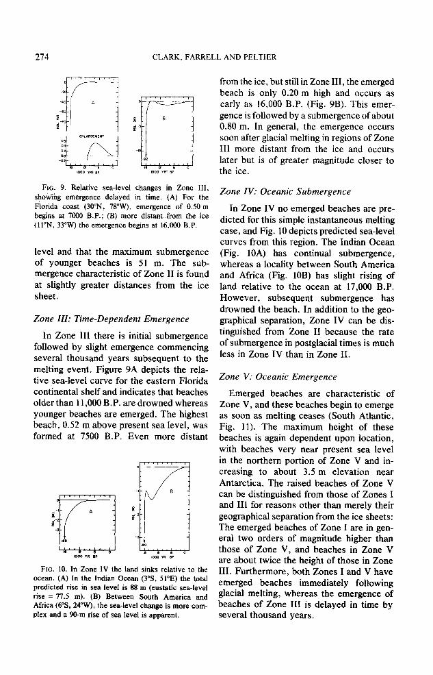
FIG. 9. Relative sea-level changes in Zone III, showihg emergence delayed in time. (A) For the dotida coast (30”N, 78”W), emergence of 0.50 m begins at 7000 B.P.; (B) more distant..from the ice (ll”N, 33”W) the emergence begins at 16,000 B.P.

level and that the maximum submergence of younger beaches is 51 m. The submergence characteristic of Zone II is found at slightly greater distances from the ice sheet.

Zone III: Time-Dependent Emergence

In Zone III there is initial submergence followed by slight emergence commencing several thousand years subsequent to the melting event. Figure 9A depicts the relative sea-level curve for the eastern Florida continental shelf and indicates that beaches older than 11,000 B.P. are drowned whereas younger beaches are emerged. The highest beach, 0.52 m above present sea level, was formed at 7500 B.P. Even more distant

FIG. 10. In Zone IV the land sinks relative to the ocean. (A) In the Indian Ocean (3”S, 51”E) the total predicted rise in sea level is 88 m (eustatic sea-level rise = 77.5 m). (B) Between South America and Africa (65, 24”W), the sea-level change is more complex and a 90-m rise of sea level is apparent.

from the ice, but still in Zone III, the emerged beach is only 0.20 m high and occurs as early as 16,000 B.P. (Fig. 9B). This emergence is followed by a submergence of about 0.80 m. In general, the emergence occurs soon after glacial melting in regions of Zone III more distant from the ice and occurs later but is of greater magnitude closer to the ice.

Zone IV: Oceanic Submergence

In Zone IV no emerged beaches are predicted for this simple instantaneous melting case, and Fig. 10 depicts predicted sea-level curves from this region. The Indian Ocean (Fig. 10A) has continual submergence, whereas a locality between South America and Africa (Fig. IOB) has slight rising of land relative to the ocean at 17,000 B.P. However, subsequent submergence has drowned the beach. In addition to the geographical separation, Zone IV can be distinguished from Zone II because the rate of submergence in postglacial times is much less in Zone IV than in Zone II.

Zone V: Oceanic Emergence

Emerged beaches are characteristic of Zone V, and these beaches begin to emerge as soon as melting ceases (South Atlantic, Fig. 11). The maximum height of these beaches is again dependent upon location, with beaches very near present sea level in the northern portion of Zone V and increasing to about 3.5 m elevation near Antarctica. The raised beaches of Zone V can be distinguished from those of Zones I and III for reasons other than merely their geographical separation from the ice sheets: The emerged beaches of Zone I are in general two orders of magnitude higher than those of Zone V, and beaches in Zone V are about twice the height of those in Zone III. Furthermore, both Zones I and V have emerged beaches immediately following glacial melting, whereas the emergence of beaches of Zone III is delayed in time by several thousand years.


2

4

i’

0

-I

kd -87

16 12 6 0 1000 YR BP

FIG. 11. The characteristic emergence of Zone V is illustrated here for a location at 235, 24”W. The 2.5 m of emergence begins immediately after the melting ceases for this uniform instantaneous melting case, and the beach formed before melting is now found at a depth of 87 m.

Zone VI: Continental Shorelines

The zones mentioned above apply only to interior regions of the oceans and not to regions on the landward margins of continental shelves. Zone VI includes all continental margins except those that lie in Zone II. Throughout Zone VI emergence occurs as soon as meltwater is no longer added to the oceans, and this emergence results from crustal tilting caused by loading of the ocean basins. As the ocean floor is depressed by the added meltwater, material within the Earth flows from under the oceans to under the continents, causing the continents to rise. As the continents rise and the oceans sink, tilting occurs at the margins of the ocean, and emergence at such locations is predicted. A typical curve for the Brazilian coastline is given in Fig. 12.

On any small island near the edge of the continental shelf in Zone IV (a zone of continual submergence) there is no emergence. Closer to the present shoreline there are locations where no postglacial submergence occurs, and at the present shoreline there are emerged beaches (Zone VI). In Zones III and V, emergence occurs on midoceanic islands as well as on continental shelves. The emergence of these continental shorelines will, in general, be greater than that found on midoceanic islands because the two effects causing emergence are combined. In Zone II, the forebulge effects of the ice

overwhelm the ocean-loading effects, so emergence on these continental shorelines is not predicted.

One assumption of the model is that the ocean area remains constant through time (i.e., the continental margins have vertical sides), but this assumption is not realistic. The rising sea will differentially load the sloping continental shelves (Chappell, 1974), and the differential loading will affect the magnitude of the emergence. Further- more, the model does not have a “lithosphere,” and this assumption will also affect the amount of tilting. The methods described in Peltier (1974) may be employed to calculate Green functions for an Earth model with a perfectly elastic lithosphere, and these will subsequently be used in a more refined ocean-loading model. The present model, therefore, will give accurate results in the southern hemisphere only for midoceanic islands. Emergence should occur in Zone VI, but the present model is not sufficiently refined to predict the amount of emergence accurately. The form of the predicted emergence, however, should be similar to the observed form.

REALISTIC DEGLACIAL HISTORY

The preceding analysis emphasized that the sea-level response to even a very simple

1000 YR BP

FIG. 12. Emergence on continental coastlines (Zone VI) is caused by crustal tilting from adjacent water loads. This emergence, shown here for the east coast of Brazil (Y’S, 37”W), is predicted for almost all continental margins. In Brazil the beach formed immediately after instantaneous uniform melting at 18,000 B.P. is now 16 m above present sea level for the instantaneous uniform-melting ice history.


glacial history can be quite complex. For a more realistic glacial history, in which glaciers melt slowly as the Earth relaxes, the sea-level response is even more con- voluted. The method we have outlined above is capable of dealing with such com- plexities, and worldwide relative sea-level changes for a realistic history of deglaciation are now considered. A rigorous test of the model is possible because its predictions can be compared to relative sea-level observations anywhere.

In this analysis, the Laurentide ice sheet is assumed to have obtained a maximum thickness of 3500 m over Hudson Bay at 16,000 B.P., the time of maximum extent of the Late Wisconsin glaciation. For the Fennoscandian ice sheet we have assumed a maximum thickness of 2700 m at that same time. We specify the ice-sheet melting histories at lOOO-year intervals, with the southern extent of the Laurentide ice sheet retreating northward followed by a rapid disintegration of the ice over Hudson Bay at 7000 B.P. Peltier and Andrews (1976) give an assumed glacial thickness for each grid point for six dates during the past 18,000 years. This study follows their history, although linear interpolation of their values was employed to determine glacial thicknesses at lOOO-year intervals. In addition, their history was shifted 2000 years in time such that the 18,000-year ice thicknesses tabulated as ICE-l (Peltier and Andrews, 1976) correspond in the present model to the 16,000-year thicknesses. The ice thicknesses at all subsequent times are similarly displaced in time. A similar adjustment in origin time was employed in the calculations of Peltier and Andrews (1976); however, the temporal resolution employed in their calculation was coarse, and ambiguities were thereby introduced. This temporal shift gives a model eustatic curve which matches observed curves more closely (e.g., Shep- ard, 1963). We assume that no ice melts after 5000 B.P., and Fig. 13 gives the eustatic rise in sea level accompanying this history of glacial melting. No change in

ocean volume occurs after 5000 B.P., and eustatic sea level in the model is never higher than at present. The total rise in global average sea level for this model is 75.6 m. Both the total rise in eustatic sea level since the last glacial maximum and the form of the sea-level curve during the past 7000 years are in dispute (Fair- bridge, 1961; Shepard, 1963; Bloom, 1970; Miimer, 1971). Fairbridge (1976) believed that eustatic sea level was higher at approximately 5000 B.P. than it is at present, whereas Bloom (1970) supported the idea that sea level has continued to rise since that time. Our model curve is a compromise between these opposing views and has the added benefit of conceptual simplicity.

For the realistic melting case only Nor- them Hemisphere ice sheets are included in the model, but retreat of the Antarctic ice sheet may have occurred as well (Hol- lin, 1962). The effects upon global sea level of possible future Antarctic ice sheet fluctu- ations were considered by Clark and Lingle (1977), and we are currently modeling the global sea-level changes due to past fluctua- tions of the Antarctic ice sheet. The model is not expected to fit all of the relative sea- level data, and we have not attempted to improve the fit by manipulating either the

FIG. 13. Model eustatic sea-level curve compared to Shepard’s (1%3) sea-level curve. In the model, eustatic sea level is never higher than at present, and no change in eustatic sea level has occurred since 5000 B.P. (i.e., the ocean volume has not changed since that time).


FIG. 14. Predicted change in sea level (in meters) since the Late Wisconsin maximum (16,000 B.P.) The melting of a realistic ice load in lOOO-year time steps since 16,008 B.P. gives this nonuniform sea-level change relative to the 16,000 B.P. shoreline for (A) 13,000, (B) 8000, (C) 5000, and (D) 0 B.P. The time-dependent sea- level change at selected localities can be compared directly to observed emergence or submergence curves.


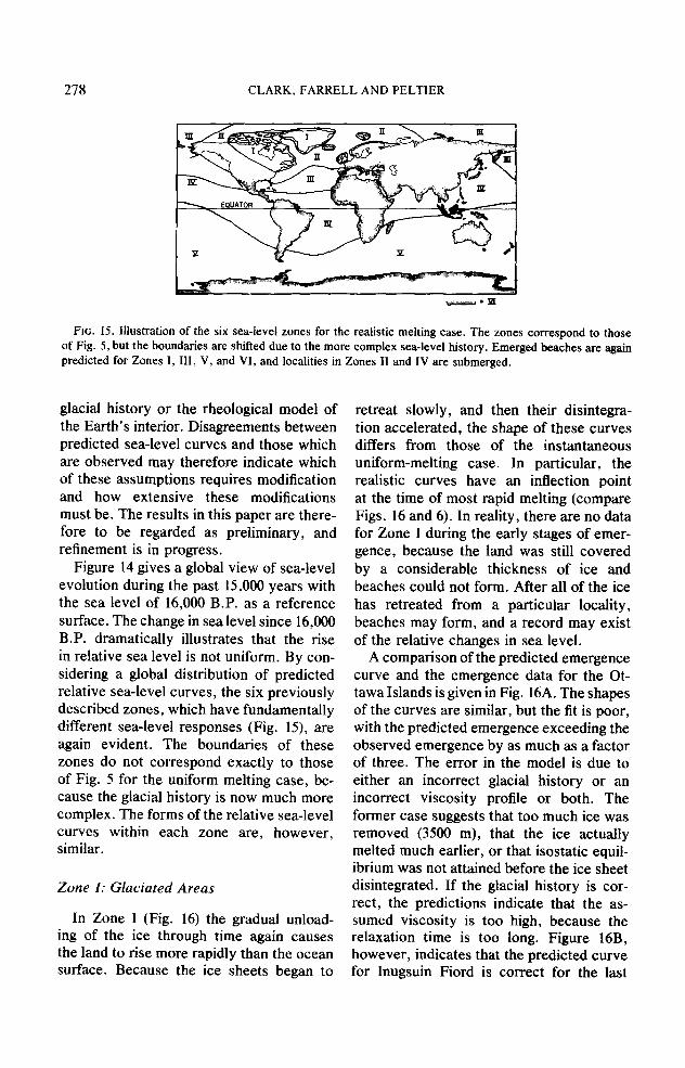
FIG. 15. Illustration of the six sea-level zones for the realistic melting case. The zones correspond to those of Fig. 5, but the boundaries are shifted due to the more complex sea-level history. Emerged beaches are again predicted for Zones I, III, V, and VI, and localities in Zones II and IV are submerged.

glacial history or the rheological model of the Earth’s interior. Disagreements between predicted sea-level curves and those which are observed may therefore indicate which of these assumptions requires modification and how extensive these modifications must be. The results in this paper are therefore to be regarded as preliminary, and refinement is in progress.

Figure 14 gives a global view of sea-level evolution during the past 15,000 years with the sea level of 16,000 B.P. as a reference surface. The change in sea level since 16,000 B.P. dramatically illustrates that the rise in relative sea level is not uniform. By considering a global distribution of predicted relative sea-level curves, the six previously described zones, which have fundamentally different sea-level responses (Fig. 15), are again evident. The boundaries of these zones do not correspond exactly to those of Fig. 5 for the uniform melting case, because the glacial history is now much more complex. The forms of the relative sea-level curves within each zone are, however, similar.

Zone I: Glaciated Areas

In Zone I (Fig. 16) the gradual unloading of the ice through time again causes the land to rise more rapidly than the ocean surface. Because the ice sheets began to

retreat slowly, and then their disintegration accelerated, the shape of these curves differs from those of the instantaneous uniform-melting case. In particular, the realistic curves have an inflection point at the time of most rapid melting (compare Figs. 16 and 6). In reality, there are no data for Zone I during the early stages of emergence, because the land was still covered by a considerable thickness of ice and beaches could not form. After all of the ice has retreated from a particular locality, beaches may form, and a record may exist of the relative changes in sea level.

A comparison of the predicted emergence curve and the emergence data for the Ot- tawa Islands is given in Fig. 16A. The shapes of the curves are similar, but the fit is poor, with the predicted emergence exceeding the observed emergence by as much as a factor of three. The error in the model is due to either an incorrect glacial history or an incorrect viscosity profile or both. The former case suggests that too much ice was removed (3.500 m), that the ice actually melted much earlier, or that isostatic equilibrium was not attained before the ice sheet disintegrated. If the glacial history is correct, the predictions indicate that the assumed viscosity is too high, because the relaxation time is too long. Figure 16B, however, indicates that the predicted curve for Inugsuin Fiord is correct for the last


5000 years, but predictions exceed observations for earlier times. If the cause is again due to the viscosity, this result, with an apparent relaxation time that is too short, suggests that the model viscosity is too low. The real lateral change in viscosity between Hudson Bay and Baffin Island is probably very slight, but the glacial history can be quite variable between these regions. We therefore believe that these errors are largely caused by an incorrect glacial history.

Peltier and Andrews (1976) did an analysis similar to that reported here and employed a similar glacial history. However, their results were in excellent agreement with the Ottawa Islands data (see also An- drews and Peltier, 1976). The differences between our prediction for the Ottawa Islands and theirs (375 m at 7000 B.P.) derive predominantly from the 2000-year shift in time between our respective ice- melting histories. Without this time shift our prediction exceeds that of Peltier and Andrews (1976) by only 170 m at 7000 B.P. Furthermore, if no water is decanted from Hudson Bay during uplift (an assumption implicit in the Peltier and Andrews calculation), then our predictions for 7000 B.P. differ by only 70 m. Also, Peltier and An- drews did not consider changes of the geoid but accounted only for the displacement of the ocean floor. Finally, as previously mentioned, their melting history was only coarsely sampled in time, whereas that employed in the present calculation had higher resolution. It is therefore not sur- prising that the two calculations differ.

The discrepancy between the present prediction and the observation at the Ottawa Islands site requires explanation. The total thickness of ice over Hudson Bay just prior to its disintegration is assumed in the model to be 2000 m. Immediately following the collapse of this central dome of the ice sheet (at 7000 B.P.), the actual thickness of water in the Bay was approximately 400 m (present depth, 200 m, plus -200 m of emergence since 7000 B.P.). In the model, how-

600 -

B .

$ 400-

1000 YRS 0P

FIG. 16. Comparison of predictions to observations in Zone I. The poor fit for (A) the Ottawa Islands (59.5”N, 8O”W; Andrews and Falconer, 1%9) and (B) Inug- suin Fiord, Baffin Island (693”N, 7O”W; Loken, 1965) suggests that the model glacial-melting history may be in error (see text for discussion).

ever, where the predicted emergence is about 500 m since 7000 B.P., the total water depth is 700 m at 7000 B.P. For there to be a total ice thickness of 2000 m at 8000 B.P., the amount of ice melted in the model would have to be on the order of 1300 m, or that portion of the ice sheet that was above sea level. In the present model the assumed total ice thickness at 8000 B.P. is then 2700 m. Reducing this value to the more reasonable value of 2000 m (- 1300 m above sea level before collapse) would have two effects, each of which would reduce the predicted emergence. The reduced effective ice load would result in a decrease


e 1000 YR BP

FIG. 17. Predictions for two localities within the Transition Zone between Zones I and II. Peat and oyster data from (A) Prince Edward Island (47”N, 6o”W; Kranck, 1972) and(B) Boston (43”N, 71”W; Kaye and Barghoom, 1964) show the characteristic emergence followed by submergence.

of the predicted emergence. This reduc- tion would, in turn, reduce the amount of water decanted from Hudson Bay, further reducing the amount of uplift. These effects will be included in future calculations, and we expect a much improved fit to the emergence curve as a consequence.

Transition Zone Between I and II: The Ice Margin

The characteristic emergence followed by submergence within the transition between Zones I and II is predicted for the Maritime Provinces and Massachusetts by the model. Here again, the ice history is very important in fitting the data. The best match for the Maritime Provinces is for Prince Edward Island (Fig. 17A).

In the Boston area the fit is worse, with much greater predicted submergence than observed (Fig. 17B). Perhaps too much ice

was melted from the Boston area in the model, and this amplified the relative sea- level effect. On the other hand, the misfit may be due in part to the lack of a lithosphere in the present model, as suggested by Peltier and Andrews (1976).

Zone II: Collapsing Forebulge Submergence

It is well known that the east coast of the United States has been submerging since at least 7000 B.P., and this submergence is predicted for the coasts of New Jersey, Virginia, and Georgia (Figs. 18A, B, and C). With the exception of Georgia, the error of fit is large, with the predicted submergence exceeding the observed submergence by a factor of two. The glacial history may again be responsible, but it is just as likely that the Earth rheology may be an important factor as the data become distant from the ice. Peltier and Andrews (1976) suggested that the Earth model used here needs modification because it does not have a perfectly elastic lithosphere. In other models (McConnell, 1968; Cathles, 1975), it has been shown that such a lithosphere will tend to decrease the amount of submergence and increase the area of Zone II. Peltier has constructed Green functions for Earth models with litho- spheres, and these are currently being employed to refine the predictions of relative sea level.

The present rates of submergence are also useful data, and Walcott (1972b) has summarized the observations. In the Gulf of Maine, New Jersey, Virginia, and Geor- gia, the predicted present rates of submergence are 3.1, 5.3, 3.9, and 0.15 mmlyr, respectively. For Maine, New Jersey, and Virginia, the rates of current submergence compare satisfactorily with the observed values. However, the total extent of the region of predicted submergence is too narrow since the Southern Georgia predicted submergence rate is much less than the observed rate of 2 mm/yr. Here is further evidence for a lithosphere that could increase the area of Zone II.


1000 YR BP

l...l...,..,,.,>, 16 I2 E 4 0

1000 YR BP

-60 -

16 I2 6 4 0 1000 YRS BP

-5o-

%

-loo- E

-150- I.. .I..,I.,,,..,, 16 n 8 4 0

1000 IRS BP

FIG. 18. Relative sea-level curves for Zone II, a zone of continuous submergence caused by the collapsing forebulge. The predicted submergence is excessive, suggesting either that the model glacial history is incorrect or that the lithosphere may be important here. (A) Brigantine, New Jersey, 39.4”N, 74.4”W (Stuiver and Daddario, 1%3); (B) Virginia, 37.6”N, 75.7”W (Harrison et al., 1%5; Newman and Rusnak, 1%5); (C) Georgia, 3l”N, 81.4”W (Wait, 1968); (D) Bermuda, 32.3”N, 64.7”W (Neumann, 1971); (E) Atlantic continental shelf, 35”N, 6TW (Emery and Garrison, 1967).


Bermuda is also in Zone II, and its midoceanic location makes it a desirable datum because it should not be affected by the crustal tilting at continental margins that may affect sites along the eastern seaboard. Figure 18D again indicates that predicted submergence exceeds observed submergence .

On the outer Atlantic shelf, the prediction once more overestimates the submergence between the present and 13,000 BP. (Fig. 18E). Before this time, it drastically underestimates the submergence by about 30 m. The results suggest that the eustatic sea-level rise may have been greater than that assumed. A eustatic rise of 103 m would

,“‘I”‘,“‘,“‘1 0.

-2o-

s-40-

% .

-60 -

-BOy

I6 I2 B 4 0 1000 YR BP

g2 o-

c J-&j- .

-6O-

1000 YR: BP

FIG. 19. Zone III sea-level curves in which emergence is delayed’k time. The emergence is so slight (<0.75 m) that it may be undetected in the sea-level record in these localities. (A) Florida, 29”N, 84”W (Scholl and Stuiver, 1%7); (B) Gulf of Mexico, 27”N, 95”W (Curray, 1960).

be necessary to fit the submerged beaches at 130 m. However, there may be considerable error in these data, and, as we shall show in the next section, the implication is con- tradicted by measurements at other sites. Either the rheological model or the deglaciation history (or both) could be contributing to this discrepancy.

Zone III: Time-Dependent Emergence

Zone III covers a very limited area of the globe, and its diagnostic feature, an emerged beach formed only a few thousand years ago, would be difficult to observe since the emergence should be (in general) less than 0.50 m above present sea level. The Florida Everglades lie on the border of this zone, and the predicted curve (19A) is close to the observed submergence. There is disagreement, however, in one detail: The model predicts slight present-day emergence (0.04 mm/yr), whereas the observations demand present-day submergence (2 mm/yr). Substantial agreement with the observations at this site was also obtained by Peltier and Andrews (1976).

The Gulf of Mexico also lies within Zone III and has a very long record of sea-level observations. Figure 19B shows that the predicted submergence is only moderately in excess of that observed. The prediction indicates a maximum submergence of 90 m with a rise in model eustatic sea level of only 75 m. For a eustatic sea-level rise of 103 m, deduced from the Atlantic continental shelf data, the predicted sea level in the Gulf of Mexico at 16,000 B.P. would be approximately 120 m. The observed level of 85 m indicates that either (1) the model is wrong, (2) the data for one of the studies is in error, or (3) tectonism is important in at least one locality.

Another locality that is within Zone III is the Aleutian Islands. The model predicts an emerged beach, 0.20 m high, that formed 2000 years ago. Powers (l%l) describes a beach 2 to 3 m above sea level that was formed 4000 to 5000 years ago on most of


-2o-

H

%

-4o-

-6O- / Ei!El .20 3 JO -

0 A -.I0 P -.20

2 zoo YR a:

Il...l.. .l...l...I I6 I2 6

1000 YR BP

FIG. 20. Sea-level change in Micronesia near the boundary of Zone IV and Zone V. The fit to the data (6.7”N, 163”E; Bloom, 1970) is excellent.

the Aleutian Islands. The regularity of the beach suggests that tectonism was not responsible for the emergence. The maximum amount of emergence predicted anywhere in Zone III is only about 0.75 m, so the Aleutian emergence may be due to some additional cause such as ice unloading (Black, 1974).

Zone IV: Oceanic Submergence

The best evidence for a region of continued submergence, distant from the ice (Zone IV), comes from Micronesia, which lies on the boundary between Zones IV and V. The predicted curve for the Marshall Islands is compared to data from Truk, Kusaie, and Ponape Islands in Fig. 20. Nu- merous rubble-topped terraces in Micro- nesia suggest that sea level may have dropped slightly until about 2000 B.P. before rising again to its present level (Shepard et al., 1967). The predicted curve indicates 0.35 m of emergence, which commenced at 5000 B.P. and was followed by submergence of 0.15 m beginning between 3000 and 2000 B.P. This matches the scenario described by Shepard et al., (1967). There is also excellent agreement with the data from Truk Island for the time period 7000 to 5000 B.P.

Much of the Indian Ocean is also in Zone IV, and Stoddart (1971) claimed that although emerged beaches ring the Indian Ocean they are absent in the central Indian Ocean. This is in excellent agreement with theory. Furthermore, Thomson and Walton (1972) believed that sea level was never higher than at present on the Aldabra Atoll north of Madagascar. This atoll is in a location relative to Zone V similar to that of Micronesia and has essentially the same form of predicted sea-level curve with about 0.15 m of emergence. It would be interest- ing to determine if the Marshall Islands and Aldabra Atoll have similar rubble- topped geomorphic features.

Zone V: Oceanic Emergence

Characteristic of Zone V is emergence that occurred as soon as the ocean volume ceased to increase. Figure 21, depicting predicted sea levels on a north-south transect across Zone V, indicates that this emergence is in general 1.5 to 2.0 m. Fur- thermore, the highest beach was formed at 5000 B.P., the time when meltwater ceased to enter the ocean basins. Figure 22 shows how the height of this 5000-B.P. beach varies with latitude between 70”s and 45”N (longitude = 165”W). It is evident that one must not simply look for a “2-m” beach or emerged reef. There are numerous claims that throughout the South Pacific old raised marine terraces approximately 5000 years old are at elevations of about 2 m (Russell, 1961). Certainly, several of these may be caused by local tectonism, but it is difficult to discount all of them. Here is further evidence to suggest that eustatic sea level stopped rising at 5000 B.P. This result also indicates that a higher eustatic sea level 5000 years ago is not necessary to explain the numerous reported emerged beaches and reefs in the South Pacific.

Zone VI: Continental Shorelines Claims of sea levels higher than present

come from essentially every continent.


I

ii II: -I

-2

-3

6 4 2 0

1000 YRS BP

2C’ ’ ’ ’ ’ ’ ‘-I

-2

- 2.N

-3

6 4 2 0 1000 YRS BP

I ’ I I I 1 I

0

-I

% --2

i -3

-4

-5

11’ ’ I L I I I 6 4 2 0

1000 YRS BP

FIG. 21. Predicted relative sea-level curves for a transect from south to north of the Pacific Ocean along the meridian 16s”W. (A) Curves indicating emergence for the region between 703 and 52%; (B) the decrease in maximum height of the 5000-B.P. beach in going from 40’5 to 2”N; (C) submergence of the MOO-B.P. beach (Zone IV) and the delayed emergence of Zone III seen in the traverse from 11”N to 44”N.

The location with perhaps the most sea- level data is Recife, Brazil (Fairbridge, 1976), and these data are typical of those found elsewhere. Figure 23 shows that the agreement between the predicted and observed variation is excellent. This site might be expected to exhibit continual submergence (Zone IV), but because of its location on the continental margin, the crustal tilting described in the uniform melting case causes emergence. The predicted curve for a region just east of Recife on the continental shelf (in Zone IV) shows the expected submergence. When the continental margin curve and the continental shelf curve are drawn superimposed upon the eustatic sea-level curve suggested by Fair- bridge (1976), the predicted curves bracket the Fairbridge curve. These predictions are for regions less than 100 km apart, and the differences in the two curves suggest that even local interpretations of relative sea level are affected by water loading.

Holocene sea-level curves from Australia and Mauritania also show a good fit to the model. Furthermore, the emerged beaches that ring the Indian Ocean (Stoddart, 1971) are also predicted. Sea-level curves from continental margins in Zone V have slightly greater emergence than those of the South Pacific islands, because continental tilting is superimposed upon the general falling of relative sea level of Zone V. Sea-level curves from the continental shelves of Mauritania and Brazil would indicate submergence (Zone IV), but such curves off the coast of Australia would indicate emergence (Zone V).

DISCUSSION

Walcott (1972a) outlined three regions where the sea-level expressions should differ: (1) rapid and large uplift under the melting ice sheet, (2) submergence peripheral to the ice sheets, and (3) coastal tilting causing emergence on continental shorelines distant from the ice. This study sup- ports these suggestions, and itself suggests


SOUTH NORTH LATITUDE

FIG. 22. Predicted height of the XlOO-B.P. beach for a transect from 70”s to 44”N along longitude 165”W in the Pacific Ocean. The height of the beach is evidently quite variable.

three additional regions not mentioned by Walcott because he decoupled the problems of ice unloading and ocean loading. The region of time-dependent emergence (Zone III) is of limited area and only modest expression in the sea level record, but it might be detected if field workers became aware of its predicted location.

The region of slight submergence (Zone IV) is recognized by the lack of emerged beaches on midoceanic islands. The central Indian Ocean is a notable example. Zone V is characterized by emerged beaches of up to 2 m that should be approximately 5000 years old. Walcott suggested that there might be similar regions, but he believed they would be defined by proximity to continents rather than proximity to the ice load. The effect of the ice certainly has a far- reaching influence. To substantiate this prediction, field data from a north-south transect of the Pacific Ocean are required.

Although agreement with observations is not perfect, the predictions of this model suggest that sea levels from all over the world may be explained without invoking any change in eustatic sea level during the past 5000 years. Any net changes in eustatic sea level during this time were probably less than 1 m, and perhaps less than 0.50 m. Such changes in eustatic sea level would be expressed as a shift of the line separating Zone IV from Zone V. For example, a net increase in eustatic sea level by 1 m since 5000 B.P. would cause the line to

shift southward approximately 22” (-2500 km) so that Zone IV is enlarged in area. Con- versely, if eustatic sea level has fallen 1 m in the past 5000 years, Zone V will be enlarged and the boundary will move approximately 44” north (-5000 km).

In the Gulf of Mexico, where a continuous record of relative sea level extends throughout the past 18,000 years, the predictions slightly overestimate the observed submergence. This suggests that the eustatic rise in sea level may have been less than 75 m, the assumed value. On the North Atlantic continental shelf the predictions underestimate observations, suggesting that the eustatic rise may have been approximately 100 m. The discrepancy is not resolved by this model, and the total rise in sea level since 18,000 B.P. is still uncertain.

Predictions of emergence for regions in glaciated areas (Zone I) are the most in error, largely due to an incorrect glacial history. It is possible to improve the fit considerably by considering the inverse problem, using the sea-level data to calculate a glacial history that is consistent with the data. This problem has been solved for an elastic Earth, and Clark (1978) has used this method to calculate ice histories for the time span 1910 to 1960 A.D. at Gla- cier Bay, Alaska. A similar inversion for the time-dependent glacial history on a viscoelastic Earth also is possible. Inversion

I. *I 1 I 4 2 0

1000 YR BP

FIG. 23. Crustal tilting from water loading causing emergence at continental shorelines (Zone VI). At Recife, Brazil (6”S, 36”W; Fairbridge, 1976), approximately 3 m of emergence is predicted (heavy line) on the coastline, whereas on the continental shelf, 100 km east of Recife, continued submergence (dashed line) characteristic of Zone IV is predicted. The fit to the data is excellent. The Fairbridge eustatic curve (light line) is bracketed by these predicted curves.


theory provides not only an efficient man- ner of fitting the data but also an estimate of the degree of departure from uniqueness of the resulting ice history and of the asso- ciated errors in the ice thickness estimates. The reconstruction of the past ice sheets from sea-level data is therefore possible.

The error of fit in the forebulge region (Zone II) is also large and may be due to an incorrect Earth rheology as well as to a faulty ice history. Peltier (1976) has constructed a theory of inference which may be employed to use the emergence (submergence) data to constrain the viscosity profile of the model. As he has described, the inverse problem is completely nonlinear since the relative sea-level data are sensi- tive to both the Earth’s rheology and to the deglaciation history. An iterative approach to the data inversion is therefore necessary. We hope this procedure will converge upon a glacial history and an Earth viscosity that is consistent with sea- level data throughout the world for the past 18,000 years.

CONCLUSION

There are no “stable” regions where eustatic sea level can be measured, because deglaciation and the addition of water to the ocean basins deform the Earth and change the observer’s point of reference. Rather, by considering the relative sea- level changes at individual locations throughout the world and comparing these observations to the predictions of a self-consistent model, it will ultimately be possible to infer a eustatic sea-level rise. Although the present model falls short of this goal, it is satisfying that in spite of its simplicity (constant eustatic sea level since 5000 B.P. and constant viscosity throughout the Earth’s mantle), it can explain a large proportion of the observed variance in the global sea-level record. The preliminary results given here serve as a general hy- pothesis that may be tested by field studies of relative sea level. Such studies will ultimately dictate the appropriate modifica-

tions of the model which are required for accurate sea-level predictions. In making these modifications, much may be learned about past glacial histories and about the rheology of the Earth’s interior.

ACKNOWLEDGMENTS

The bulk of this work was accomplished at the University of Colorado, where the support of the Cooperative Institute for Research in Environmental Sciences (CIRES) and the Institute of Arctic and Alpine Research (INSTAAR) was very beneficial to us. John T. Andrews has greatly aided us throughout this study, and discussions with John T. Hollin, Craig S. Lingle, and Arthur L. Bloom were of considerable benefit. We also appreciate the help of Keith Echel- meyer, who helped us write a portion of the computer code, and P. Tom Davis, who compiled sea-level data from the literature. Some of the computer time for this project was donated by the computing centers of the National Oceanic and Atmospheric Administration (Boulder Laboratory) and the University of Colorado. Acknowledgment is also made to the National Center for Atmospheric Research, which is sponsored by the National Science Foundation, for additional computer time. Funds for this work were provided by the National Science Foundation under Grants DES74- 13047-A01 and EAR7413047-A02 to CIRES and Grant EAR77-13662 to the Department of Geological Sciences, Cornell University.

REFERENCES

Alterman, Z., Jarosch, H., and Pekeris, C. L. (1961). Propagation of Rayleigh waves in the Earth. Geo- phys. J.R. astr. Sot. 4, 219-241.

Andrews, J. T., and Falconer, G. (1969). Late glacial and postglacial history and emergence of the Ottawa Islands, Hudson Bay, N.W.T.: Evidence on the deglaciation of Hudson Bay. Canad. J. Earth Sci. 6, 1263-1276.

Andrews, J. T., and Peltier, W. R. (1976). Collapse of the Hudson Bay ice center and glacio-isostatic rebound. Geology 4, 73-75.

Black, R. F. (1974). Late Quatemary sea-level changes, Umnak Island, Aleutians: Their effects on ancient Aleuts and their causes. Quaternary Res. 4,264-281.

Bloom, A. L. (1967). Pleistocene shorelines: A new test of isostasy. Geol. Sot. Amer. Bull. 78, 1477- 1494.

Bloom, A. L. (1970). Pahtdal stratigraphy of Truk, Ponape, and Kusaie, Eastern Caroline Islands. Geoi. Sot. Amer. Bull. 81, 1895-1904.

Cathles, L. M. (1975) “The Viscosity of the Earth’s MantIe,” 386 pp. Princeton University Press, Prince- ton, N. J.

Chappell, J. (1974). Late Quatemary glacio- and


hydro-isostasy on a layered Earth. Quaternary Res. 4, 429-440.

Clark, J. A. (1976). Greenland’s rapid postglacial emergence: A result of ice-water gravitational attraction. Geology 4, 310-312.

Clark, J. A. (1978). An inverse problem in glacial geology: The reconstruction of glacier thinning in Glacier Bay, Alaska, between 1910 and 1960 A.D. from relative sea-level data. J. of G/a&logy.

Clark, J. A., and Lingle, C. S. (1977). Future sea- level changes due to West Antarctic ice sheet Ruc- tuations. Nature 269, 206-209.

Curray, J. R. (1960). Sediments and history of Holo- cene transgression, Continental Shelf, Northwest Gulf of Mexico. In “Recent Sediments N.W. Gulf of Mexico” (F. P. Shepard et al., Eds.). Tulsa Amer. Assoc. Petro. Geol., pp. 221-266.

Daly, R. A. (1934). “The Changing World of the Ice Age,” 272 pp. Yale University Press, New Haven, Corm.

Emery, K. O., and Garrison, L. E. (1%7). Sea levels 7000 to 20,000 years ago. Science 157, 684-687.

Fairbridge, R. W. (l%l). Eustatic changes in sea level. Phys. Chem. Earth 4, 99- 185.

Fairbridge, R. W. (1976). Shellfish-eating preceramic Indians in coastal Brazil. Science 191, 353-359.

Farrell, W. E. (1972). Deformation of the Earth by surface loads. Rev. Geophys. and Space Phys. 10, 761-797.

Farrell, W. E., and Clark, J. A. (1976). On postglacial sea level. Geophys. J.R. astr. Sot. 46, 647-667.

Gill, E. D. (1965). Radiocarbon dating of past sea levels in SE Australia. Abstracts, INQUA VII Congress, Boulder, Colorado, p. 167.

Harrison, W., Malloy, R. J., Rusnak, G. A., and Teras- mae, J. (1965). Possible late Pleistocene uplift Chesa- peake Bay entrance. J. Geology 73, 201-229.

Hollin, J. T. (1962). On the glacial history of Antarctica. J. of Glaciology 4, 173- 195.

Jelgersma, S., (1966). Sea-level changes during the last 10,000 years. In “Proceedings of the Intema- tional Symposium on World Climate from 8000 to 0 B.C.,” pp. 54-71, Roy. Meteor. Sot., London.

Kaye, C. A., and Barghoom, E. S. (1964). Late Quater- nary sea-level change and crustal rise at Boston, Mass., with notes on the autocompaction of peat. Geol. Sot. Amer. Bull. 75, 63-80.

Kranck, K. (1972). Geomorphological development and post-Pleistocene sea-level changes, Northumberland Strait, Maritime Provinces. Canad. J. Earth. Sci. 9, 835-844.

Loken, 0. H. (1965). Postglacial emergence at the south end of Inugsuin fiord, Baflin Island, N.W.T. Geogr. Bull. 7, 243-258.

McConnell, R. K. (1%8). Viscosity of the mantle from relaxation time spectra of isostatic adjustment. J. Geophys. Res. 73, 7089-7105.

Mamer, N. (1971). Eustatic changes during the last

20,000 years and a method of separating the isostatic and eustatic factors in an uplifted area. Palueogeo- graphy, Palaeoclimatology, and Palaeoecology 9, 153-181.

Neumann, C. A. (1971). Quaternary sea-level data from Bermuda. Quaternariu 14, 41-43.

Newman, W. S., and Rusnak, G. A. (1965). Holocene submergence of the eastern shore of Virginia. Science 148, 1464- 1466.

Peltier, W. R. (1974). The impulse response of a Maxwell Earth. Rev. Geophys. and Space Phys. 12, 649-705.

Peltier, W. R. (1976). Glacial-isostatic adjustment II: The inverse problem. Geophys. J.R. astr. Sac. 46, 669-705.

Peltier, W. R., and Andrews, J. T. (1976). Glacial- isostatic adjustment I: The forward problem. Geo- phys. J.R. astr. Sot. 46, 605-646.

Powers, H. A. (1961). The emerged shorelines at 2-3 meters in the Aleutian Islands. Zeit. Geomorph. Suppl. 3, 36-38.

Russell, R. J., Ed. (1961). Pacific Island Terraces: Eustatic? Zeit. Geomorph. Suppl. 3, 106 pp.

Schofield, J. C. (1964). Post-glacial sea levels and isostatic uplift. N.Z. J. Geol. Geophys. 7, 359-370.

Scholl, D. W., and Stuiver, M. (1967). Recent submergence of southern Florida: A comparison with adjacent coasts and other eustatic data. Geol. Sot. Amer. Bull. 78, 437-454.

Shepard, F. P. (1963). 35,000 years of sea level. In “Essays in Marine Geology,” pp. l- 10. Univ. Southern California Press, Los Angeles, Calif.

Shepard, F. P., Curray, J. R., Newman, W. A., Bloom, A. L., Newell, N. D., Tracey, J. I. Jr., and Veeh, H. H. (1967). Holocene changes in sea level in Micronesia. Science 157, 542-544.

Stoddart, D. R. (1971). Environment and history in Indian Ocean reef morphology. In “Regional Varia- tion in Indian Ocean Coral Reefs” (D. R. Stoddart and Sir Maurice Younge, Eds.), pp. 3-28. Pub- lished for Zoological Sot. of London by Academic Press, London.

Stuiver, M., and Daddario, J. J. (1963). Submergence of the New Jersey coast. Science 142, 951.

Thomson, J., and Walton, A. (1972). Redetermination of chronology of Aldabra atoll by *3”Th-234U dating. Nature 240, 145-146.

Wait, R. L. (1968). Submergence along the Atlantic Coast of Georgia. USGS Prof. Paper, 600-D, pp. 38-41.

Walcott, R. I. (1972a). Past sea levels, eustasy and deformation of the Earth. Quaternary Res. 2, l- 14.

Walcott, R. I. (1972b). Late Quatemary vertical movements in eastern North America: Quantitative evidence of glacio-isostatic rebound. Rev. of Geo- phys. and Space Phys. 10, 849-884.

Wellman, H. W. (1964). Delayed isostatic response and high sea levels. Nature M2, 1322- 1323.

Documents

Global Changes in Postglacial Sea Level: A Numerical