Global Climate ChangeGlobal Climate Change

Observations of modern global change

Climate models

Projections of future global change

Changing the Atmospheric Changing the Atmospheric Emissivity!Emissivity!

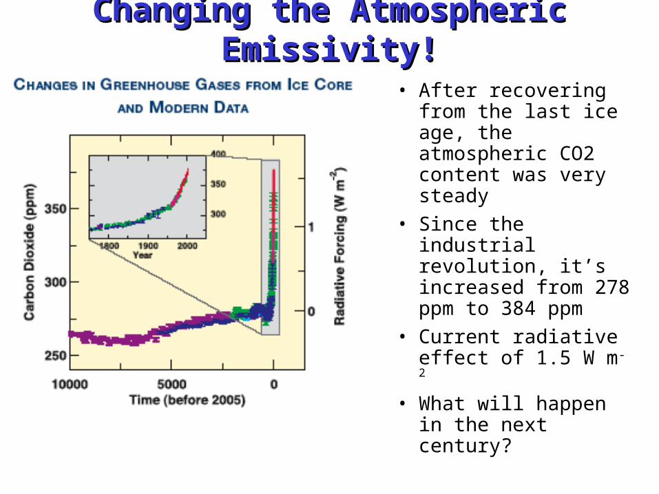
• After recovering from the last ice age, the atmospheric CO2 content was very steady

• Since the industrial revolution, it’s increased from 278 ppm to 384 ppm

• Current radiative effect of 1.5 W m-2

• What will happen in the next century?

Anthropogenic ForcingAnthropogenic Forcing

140 Years 140 Years of Dataof Data

Aerosol-Cloud Albedo FeedbackAerosol-Cloud Albedo Feedback

• Ship tracks off west coast

• Aerosol serves as CCN

• Makes more/smaller cloud drops

• Higher albedo

Atmospheric Atmospheric AerosolAerosol

Radiative-Convective Radiative-Convective EquilibriumEquilibrium

Manabe and Wetherald (1967)

stratospheric cooling

tropospheric cooling

Vertical Vertical StructureStructure

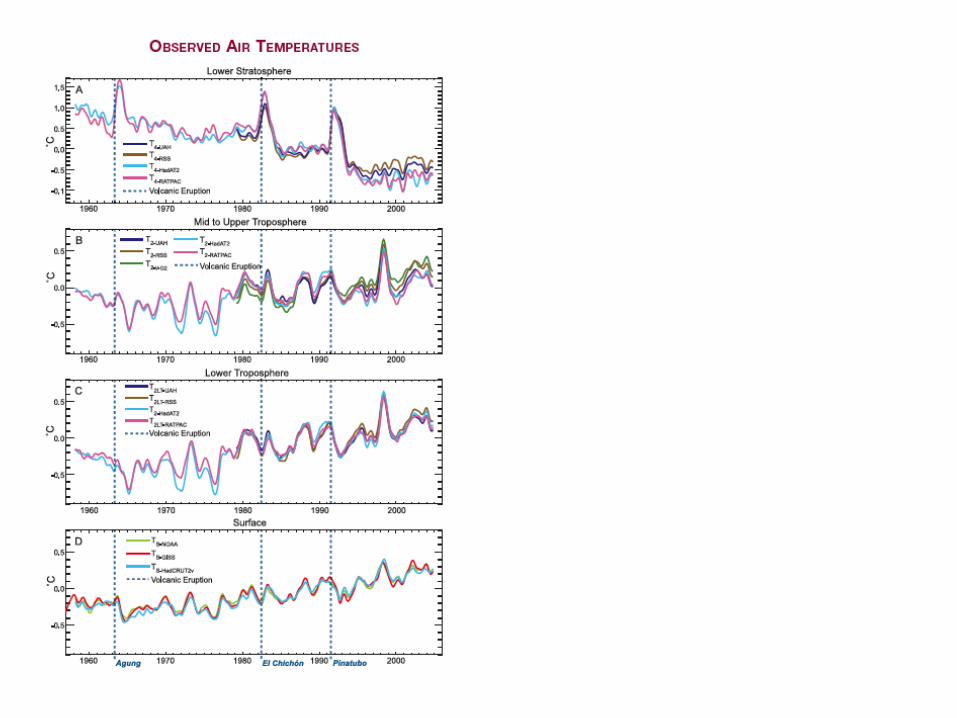
• Greenhouse “signature” is tropospheric warming and stratospheric cooling

Temperature IndicatorsTemperature Indicators

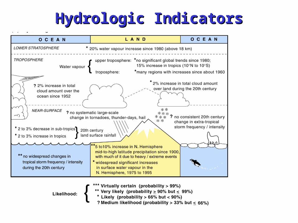
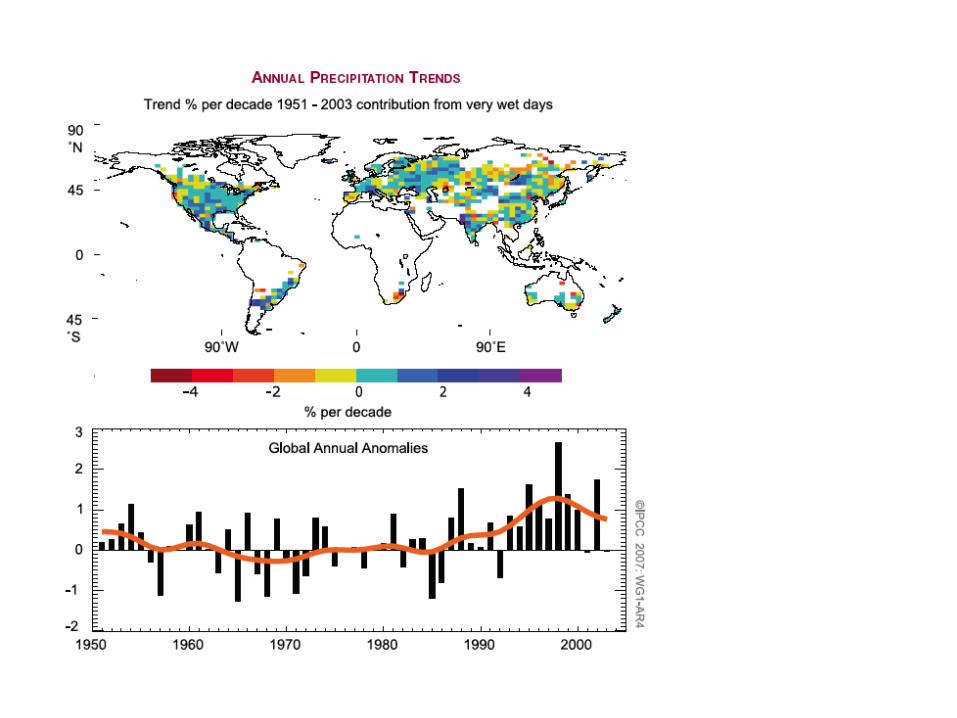
Hydrologic IndicatorsHydrologic Indicators

Climate ModelsClimate Models

Climate Model StructureClimate Model Structure

Evolution of Climate ModelsEvolution of Climate Models

Climate Model Grid CellsClimate Model Grid Cells

• Recent global NWP models typically use dx ~ 50 km

• Typical climate models dx ~ 200 km

Climate Model Vertical Climate Model Vertical StructureStructure

• 9-level model c. 1970

• Recent weather prediction models use ~60 levels, up to 1 mb

• Climate models typically somewhat coarser

Resolution and Resolution and ParameterizationParameterization

CMMAPCMMAP

CCSMCCSM

Change in TOA Cloud Change in TOA Cloud Radiative Forcing for Radiative Forcing for

2xCO2 2xCO2

Change in the Top of the Atmosphere (TOA) Cloud Radiative Forcing (CRF) associated with a CO2 doubling (from a review by Le Treut and McAvaney, 2000). The models are coupled to a slab ocean mixed layer and are brought to equilibrium for present climatic conditions and for a double CO2 climate. The sign is positive when an increase of the CRF (from present to double CO2 conditions) increases the warming, negative when it reduces it.

Water Vapor Feedback and Water Vapor Feedback and CloudsClouds

Relationship between simulated global annually averaged variation of net cloud radiative forcing at the top of the atmosphere and precipitable water due to CO2 doubling produced in simulations with different parameteriz-ations of cloud related processes.

Ocean-Atmosphere CouplingOcean-Atmosphere Coupling

• CFL Stability criteria

• Spatial scales

• Time scales

• Asynchronous coupling

• Flux correction

Sea Ice is Complicated!Sea Ice is Complicated!

• Changes in albedo, thickness, heat fluxes, water vapor flux at sfc

• Freezing, thawing, advection, interaction with ocean currents

Sea Ice Temperatures Sea Ice Temperatures and Heat Fluxesand Heat Fluxes

Land-Atmosphere CouplingLand-Atmosphere Coupling

• Schematic showing relationships between a simulation of the Atmospheric Boundary Layer (ABL), a Land-Surface Parametrization (LSP), vegetation and soil properties, and anthropogenic change. Interactions are shown by broad white arrows marked with capital letters, fluxes by grey arrows, and dependencies by dotted lines.

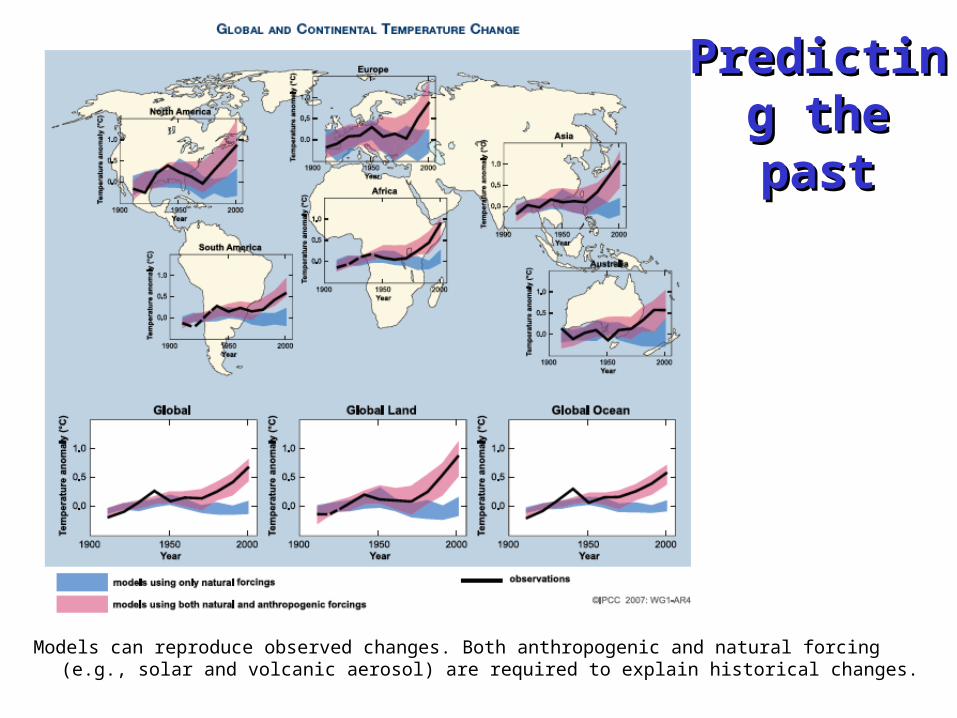
Models can reproduce observed changes. Both anthropogenic and natural forcing (e.g.,

solar and volcanic aerosol) are required to explain historical changes.

PredictinPredicting the g the pastpast

Signal:NoisSignal:Noisee

Projections of the FutureProjections of the Future

Means and Means and VariancesVariances

Schematic showing the effect on extreme temperatures when (a) the mean temperature increases, (b) the variance increases, and (c) when both the mean and variance increase for a normal distribution of temperature.

Emission ScenariosEmission Scenarios

Recent emissions

1990 1995 2000 2005 2010

5

6

7

8

9

10Actual emissions: CDIACActual emissions: EIA450ppm stabilisation650ppm stabilisationA1FI A1B A1T A2 B1 B2

1850 1900 1950 2000 2050 2100

0

5

10

15

20

25

30Actual emissions: CDIAC450ppm stabilisation650ppm stabilisationA1FI A1B A1T A2 B1 B2

Emission Scenarios vs RealityEmission Scenarios vs Reality

Recent emissions

1990 1995 2000 2005 2010

5

6

7

8

9

10Actual emissions: CDIACActual emissions: EIA450ppm stabilisation650ppm stabilisationA1FI A1B A1T A2 B1 B2

1850 1900 1950 2000 2050 2100

0

5

10

15

20

25

30Actual emissions: CDIAC450ppm stabilisation650ppm stabilisationA1FI A1B A1T A2 B1 B2

Raupach et al. 2007 PNAS

Future Climate SimulationsFuture Climate Simulations

• Some warming is “committed”

• Emissions

• Uncertainty

Accelerated Hydrologic CycleAccelerated Hydrologic Cycle

Wet places get wetter (ITCZ, midlats), and dry places get drier (subtropical highs)

Climate ImpactsClimate Impacts

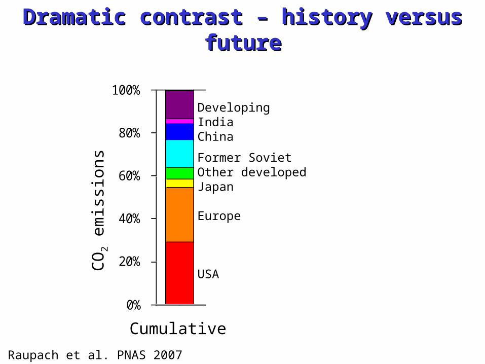
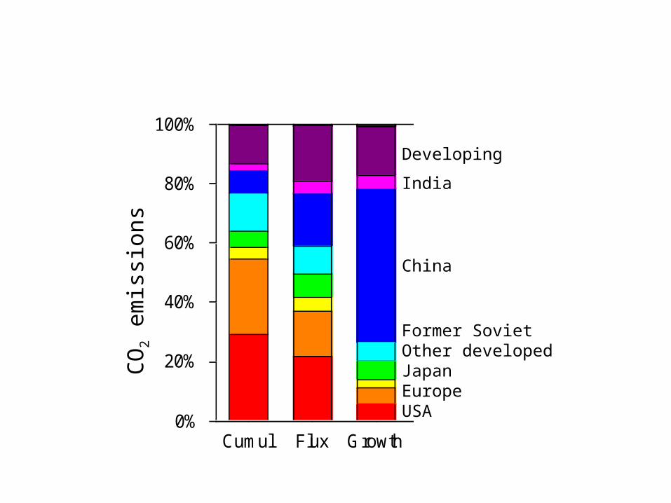
Dramatic contrast – history versus Dramatic contrast – history versus futurefuture

Cumul Flux Growth Pop0%

20%

40%

60%

80%

100%D3

India

D2

China

FSUD1

JapanEUUSA

CO

2 e

mis

sion

sDevelopingIndiaChina

Former SovietOther developedJapan

Europe

USA

Cumulative

Raupach et al. PNAS 2007

Cumul Flux Growth Pop0%

20%

40%

60%

80%

100%D3

India

D2

China

FSUD1

JapanEUUSA

CO

2 e

mis

sion

sDeveloping

India

China

Former Soviet

Other developedJapan

Europe

USA

Cumul Flux Growth Pop0%

20%

40%

60%

80%

100%D3

India

D2

China

FSUD1

JapanEUUSA

CO

2 e

mis

sion

sDeveloping

India

China

Former SovietOther developedJapanEuropeUSA

Cumul Flux Growth Pop0%

20%

40%

60%

80%

100%D3

India

D2

China

FSUD1

JapanEUUSA

CO

2 e

mis

sion

sLeast Developed

Developing

India

China

Former SovietOther developedJapanEuropeUSA

Carbon intensity of the world Carbon intensity of the world economy fell steadily for 30 yearseconomy fell steadily for 30 years

Canadell et al. 2007

Until 2000!Until 2000!

Canadell et al. 2007

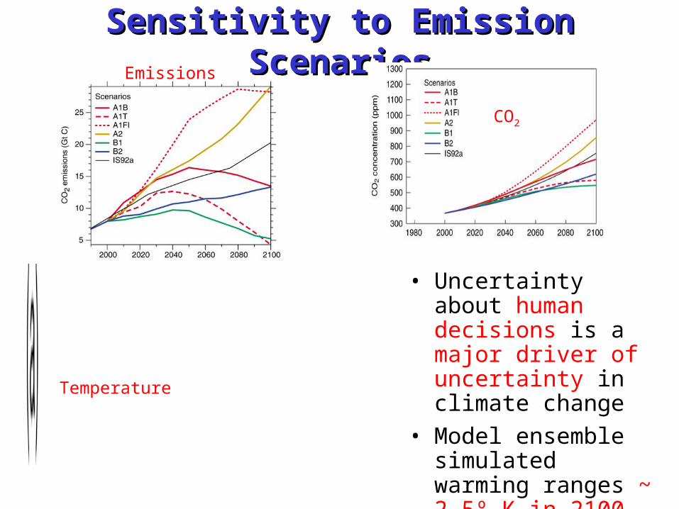
• Uncertainty about human decisions is a major driver of uncertainty in climate change

• Model ensemble simulated warming ranges ~ 2.5º K in 2100

Sensitivity to Emission Sensitivity to Emission ScenariosScenariosEmissions

CO2

Temperature

CO2 CO2 StabilizatioStabilizatio

n?n?

Only about 40% of the emissions Only about 40% of the emissions stay in the atmospherestay in the atmosphere

• Atmosphere = 42%– +0.0011/yr

• Oceans = 30%– -0.0005/yr

• Land =27%– -0.0006/yr

• Subsidy fromland & oceans

Canadell et al. 2007

The Global Carbon CycleThe Global Carbon Cycle

Humans

Atmosphere

760 + 3/yr

Ocean

38,000

Land

2000

~90

~120

~120

7 GtC/yr

~90

About half the CO2 released by humans is absorbed by oceans and land

“Missing” carbon is hard to find among large natural fluxes

European Climate ExchangeEuropean Climate ExchangeFutures Trading: Permits to Emit CO2Futures Trading: Permits to Emit CO2

• European “cap-and-trade” market set up as described in Kyoto Protocol

• About €20/ton of CO2 = $101/ton of carbon

ECX CFI Futures Contracts: Price and Volume

0

2,000,000

4,000,000

6,000,000

8,000,000

10,000,000

12,000,000

2/7/102/28/103/21/104/11/105/4/105/25/106/16/107/7/107/28/108/18/109/8/109/29/1010/20/1011/10/1012/1/1012/22/1016/01/201106/02/201127/02/201120/03/201111/04/201102/05/201123/05/201113/06/201104/07/2011

VOLUME (tonnes CO2)

0.00

5.00

10.00

15.00

20.00

25.00

30.00

35.00

Price per tonne (EUR)

Total VolumeDec07 SettDec08 Sett

The “Missing Sink”The “Missing Sink”

• Terrestrial and marine exchanges currently remove more than 4 GtC per year from the atmosphere

• This free service provided by the planet constitutes an effective 50% emissions reduction, worth $400 Billion per year at today’s price on the ECX!

• Science is currently unable to quantitatively account for – The locations at which these sinks operate– The mechanisms involved– How long the carbon will remain stored – How long the sinks will continue to operate– Whether there is anything we can do to make them

work better or for a longer time

Where Has All the Carbon Where Has All the Carbon Gone?Gone?

• Into the oceansoceans– Solubility pump (CO2 very soluble in cold water,

but rates are limited by slow physical mixing)– Biological pump (slow “rain” of organic debris)

• Into the landland– CO2 Fertilization

(plants eat CO2 … is more better?)– Nutrient fertilization

(N-deposition and fertilizers)– Land-use change

(forest regrowth, fire suppression, woody encroachment … but what about Wal-Marts?)

– Response to changing climate (e.g., Boreal warming)

Coupled Carbon Cycle Climate Coupled Carbon Cycle Climate ModelingModeling

• “Earth System” Climate Models– Atmospheric GCM– Ocean GCM with biology and chemistry– Land biophysics, biogeochemistry, biogeography

• Prescribe fossil fuel emissions, rather than CO2 concentration as usually done

• Integrate model from 1850-2100, predicting both CO2 and climate as they evolve

• Oceans, plants, and soils exchange CO2 with model atmosphere

• Climate affects ocean circulation and terrestrial biology, thus feeds back to carbon cycle

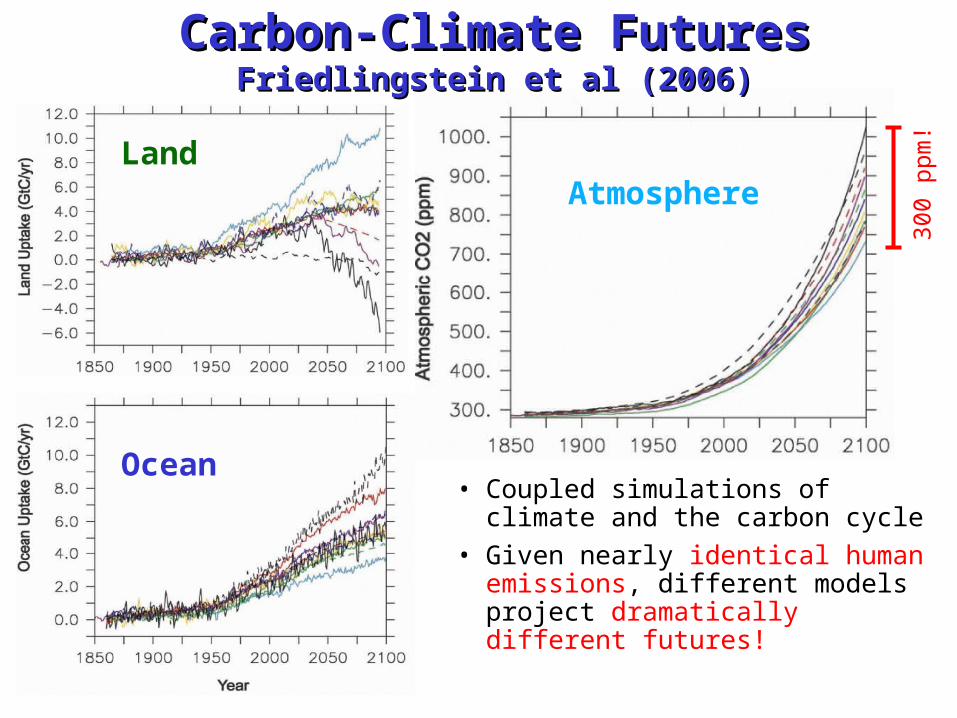
• Coupled simulations of climate and the carbon cycle

• Given nearly identical human emissions, different models project dramatically different futures!

Land

Ocean

Atmosphere 30

0 pp

m!

Carbon-Climate FuturesCarbon-Climate FuturesFriedlingstein et al (2006)Friedlingstein et al (2006)