GLOBAL LIVESTOCK ENVIRONMENTAL ASSESSMENT MODEL interactive€¦ · 3. STEP-BY-STEP EXAMPLE ... HERD MODULE ... GLEAM-i is based on the Global Livestock Environmental Assessment Model

GLOBAL LIVESTOCK ENVIRONMENTAL

ASSESSMENT MODEL - interactive

A tool for estimating livestock production, greenhouse gas emissions and assessing intervention scenarios

VERSION 2.0

Revision 3

March 2017

USER GUIDE

The designations employed and the presentation of material in this information product do not imply the expression of any opinion whatsoever on the part of the Food and Agriculture Organization of the United Nations (FAO) concerning the legal or development status of any country, territory, city or area or of its authorities, or concerning the delimitation of its frontiers or boundaries. The mention of specific companies or products of manufacturers, whether or not these have been patented, does not imply that these have been endorsed or recommended by FAO in preference to others of a similar nature that are not mentioned. The views expressed in this information product are those of the author(s) and do not necessarily reflect the views or policies of FAO. © FAO, 2017 FAO encourages the use, reproduction and dissemination of material in this information product. Except where otherwise indicated, material may be copied, downloaded and printed for private study, research and teaching purposes, or for use in non-commercial products or services, provided that appropriate acknowledgement of FAO as the source and copyright holder is given and that FAO’s endorsement of users’ views, products or services is not implied in any way. All requests for translation and adaptation rights, and for resale and other commercial use rights should be made via www.fao.org/contact-us/licence-request or addressed to [email protected]. FAO information products are available on the FAO website (www.fao.org/publications) and can be purchased through [email protected].

http://www.fao.org/contact-us/licence-request

mailto:[email protected]

http://www.fao.org/publications

mailto:[email protected]

Table of Contents 1. INTRODUCTION ........................................................................................................................................ 1

1.1. USER’S GUIDE CONTENT ..................................................................................................................... 1

1.2. KEY CONCEPTS AND TERMINOLOGY ...................................................................................................... 1

1.3. GLEAM-i STRUCTURE OVERVIEW ........................................................................................................ 2

1.4. SOURCES OF EMISSIONS ..................................................................................................................... 3

1.5. TARGETED USERS .............................................................................................................................. 4

2. GLEAM-i IN DETAIL ............................................................................................................................... 5

2.1. GENERAL ASPECTS ............................................................................................................................. 5

2.2. START PAGE ..................................................................................................................................... 8

2.3. MODULES DESCRIPTION: HERD MODULE ............................................................................................... 9

2.4. MODULES DESCRIPTION: FEED MODULE .............................................................................................. 10

2.5. MODULES DESCRIPTION: MANURE MODULE ........................................................................................ 13

2.6. RESULTS PAGES ............................................................................................................................... 14

3. STEP-BY-STEP EXAMPLE ...................................................................................................................... 19

3.1. SETTING THE BASELINE ..................................................................................................................... 19

3.2. SCENARIO DESCRIPTION .................................................................................................................... 19

3.3. IMPLEMENTING THE SCENARIO: HERD MODULE .................................................................................... 21

3.4. IMPLEMENTING THE SCENARIO: FEED MODULE ..................................................................................... 23

3.5. IMPLEMENTING THE SCENARIO: MANURE MODULE ............................................................................... 25

3.6. BASELINE AND SCENARIO COMPARISON ............................................................................................... 26

3.7. SAVING THE RESULTS ....................................................................................................................... 27

4. ANNEX ................................................................................................................................................. 28

1

1. INTRODUCTION 1.1. USER’S GUIDE CONTENT This user guide describes how to use the Global Environmental Assessment Model-interactive tool (GLEAM-i) to

estimate production, greenhouse gas (GHG) emissions and mitigation potential in livestock supply chains. GLEAM-i

is intended to support policy-makers, private sector, NGOs, scientists and civil society in understanding emissions

from livestock production and designing interventions to reduce their contribution to climate change.

This user guide is divided into three chapters and one annex:

- Introduction: provides a brief introduction to key concepts and terminology, describes the general

structure of the model and discusses the targeted public of the tool.

- GLEAM-i in detail: describes the livestock production systems covered by GLEAM-i and explains the

different modules of the tool.

- Step-by-step example: provides a detailed example on how to implement a scenario.

- Annex: detailed lists of variables in GLEAM-i.

1.2. KEY CONCEPTS AND TERMINOLOGY GREENHOUSE GAS EMISSIONS AND GLOBAL WARMING POTENTIAL

GLEAM-i covers the emissions of the three main GHG related to agricultural activities: carbon dioxide (CO2), methane

(CH4) and nitrous oxide (N2O). The Global Warming Potential (GWP) is the measure of the ability of a certain gas to

trap heat in the atmosphere for a given period of time relative to a CO2 molecule. GLEAM-i uses the 100 years AR5

IPCC report1 GWP values: 34 for CH4 and 298 for N2O. That is to say that molecules of methane and nitrous oxide

trap respectively 34 and 298 times more heat than carbon dioxide over a period of 100 years.

USE OF IPCC TIER 2 METHODOLOGIES

A given IPCC Tier refers to a set of methodological rules used to estimate GHG emissions with an increasing level of

complexity2. GLEAM-i uses Tier 2 methodologies to perform most of its calculations. In contrast with the simpler Tier

1 approach, Tier 2 methods rely on enhanced characterization of animal populations. This translates into a more

accurate estimation of feed intake and quality for the calculation of emissions from enteric fermentation and manure

management. Also, the use of Tier 2 methodologies better reflects changes in emissions due to intervention

scenarios such as feed or manure management.

LIFE CYCLE ASSESSMENT

The general principle of a life cycle assessment (LCA) is to account for all the inputs and outputs associated with a

specific product within a defined boundary system. The application of LCA allows the detection of negative

environmental burdens along the main stages of livestock production. It also allows to identify when interventions

would result in shifting the negative effects from one stage to another.

DEFAULT, BASELINE AND SCENARIO CONDITIONS

Default conditions are those included in the tool database and are calculated as country averages of the values used

in the main GLEAM model. Baseline conditions represent the “initial” system state, that is, the situation to which the

Scenario conditions will be compared to. Scenario conditions refers to the situation where changes to the Baseline

conditions have been made (to simulate a mitigation package, for instance). Before any modifications, all three sets

of values are identical.

1 IPCC, 2014. Climate change 2014: Synthesis report. IPCC, Geneva. 2 IPCC, 2006. Guidelines for National Greenhouse Gas Inventories. IPCC, Geneva

GLEAM-i INTRODUCTION Revision 3 – March 2017

2

1.3. GLEAM-i STRUCTURE OVERVIEW GLEAM-i is based on the Global Livestock Environmental Assessment Model (GLEAM), a spatially explicit modelling

framework that simulates the biophysical processes of livestock production and its environmental impacts using a

LCA approach. GLEAM differentiates key stages along livestock supply chains such as feed production, processing

and transport, herd dynamics, animal feeding and manure management.

GLEAM-i retains most of the key characteristics of GLEAM:

- Coverage of six livestock species and their edible products: meat and milk from cattle, buffalo, sheep and

goats; meat from pigs and meat and eggs from chicken.

- Estimation of CO2, CH4 and N2O emissions arising from each stage of production.

- Use of Tier 2 methodology in animal herd dynamics, enteric fermentation and manure management

emissions, providing accurate information on how animal husbandry, feeding and manure management

options affect environmental performance.

- Use of 2010 data in GLEAM-i 2.0 and a number of new features also added in GLEAM 2.0 such as CO2

emissions due to land-use change for production of palm kernel cakes and addition of a new production

system: feedlot operations for beef cattle.

Users can find detailed description of GLEAM, including variables and equations, in the GLEAM model description

on line.

GLEAM-i consists of three modules for data input, representing the main livestock production stages and one

calculation module (Figure 1). The purpose of each module is summarized below:

- The herd module simulates the herd dynamics and the average animal characteristics for each cohort.

- The feed module determines the nutritional characteristics of diets and estimates the associated emissions.

- The manure module calculates the rate at which nitrogen from manure is deposited and applied in the

fields. This is necessary to calculate emissions associated with feed production.

- Total herd emissions and production are calculated in the system module using Tier 2 methods.

http://www.fao.org/fileadmin/user_upload/gleam/docs/GLEAM_2.0_Model_description.pdf


3

Figure 1. Schematic representation of GLEAM-i, showing the main modules, input data and calculation flows.

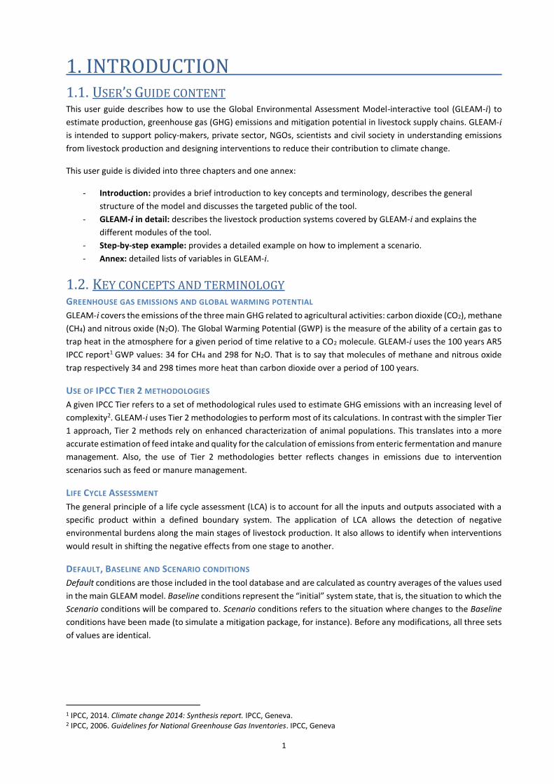
1.4. SOURCES OF EMISSIONS GLEAM-i covers the emissions from the three major GHGs associated with animal food chains: methane (CH4),

nitrous oxide (N2O) and carbon dioxide (CO2). Table 1 presents the emissions sources included in GLEAM-i.

Note that, in contrast with GLEAM, ‘Postfarm’ emissions (that is, CO2 emissions from the postfarm processing and

transport of livestock products) is not included in GLEAM-i. The reason to exclude them is that data needed to

estimate those emissions is rarely available at country level, making the estimation highly uncertain below a regional

or sub-continental scope.

HERD MODULE

Calculates:

The structure of the herd

The characteristics of the animals in

each cohort

FEED MODULE

Calculates:

Emissions and nutritional values

per kg of ration

Share of each feed type in the ration

MANURE MODULE

Calculates:

The amount of manure deposited on

pastures and applied to fields

Number reproductive adult animals

Herd parameters: fertility, mortality

and replacement rates

Share of manure treated in each

manure management system

PRODUCTION DATA

Animal numbers, meat, milk and eggs

EMISSION DATA

Total emissions, emissions by gas, species, source

SYSTEM MODULE

Calculates:

Total emissions from feed

Total emissions from enteric fermentation

Total emissions from manure management

Total production of meat, milk, eggs

Total animal numbers

Average weight and growth rates

Gross, digestible and metabolizable energy per kg of ration

Nitrogen per kg of ration

Emissions per kg of ration

User defined input

Calculation module

Intermediate result

Final results

Amount of manure deposited on pastures and applied to fields


4

TABLE 1. Emission sources covered in GLEAM-i Source of emissions Description FEED: production (N2O)

applied and deposited manure

N2O emissions from the conversion of nitrogenous compounds present in animal excreta: manure can be deposited in the fields by grazing and scavenging animals or applied to feed crop fields as organic fertilizer. It includes direct emissions (conversions of nitrogen into N2O through a combination of nitrification and denitrification processes) and indirect emissions (nitrogen is lost in forms of ammonia and NOx).

fertilizer and crop residues

N2O emissions from the conversion of nitrogenous compounds present in synthetic nitrogenous fertilizers applied to feed crops and from the decomposition of crop residues. It includes direct emissions (conversions of nitrogen into N2O through a combination of nitrification and denitrification processes) and indirect emissions (nitrogen is lost in forms of ammonia and NOx).

FEED: production (CO2)

production CO2 emissions arising from the production, transport and processing of feed. This includes emissions from fossil fuels use in fertilizer and pesticides manufacture, field operations and feed manufacture in feed mills.

FEED: land-use change (CO2)

soybean cultivation

CO2 emissions due to the expansion of soybean cultivation into natural areas. Emissions are related to changes in carbon stored in biomass, dead organic matter and soils.

palm kernel cake

CO2 emissions due to the expansion of palm oil plantations into natural areas. Emissions are related to changes in carbon stored in biomass, dead organic matter and soils.

pasture expansion

CO2 emissions due to the expansion of pastures into natural areas. Emissions are related to changes in carbon stored in biomass, dead organic matter and soils.

FEED: methane (CH4) CH4 emissions from the cultivation of rice used as feed. Emissions are related to anaerobic decomposition of organic matter in flooded rice fields.

ENTERIC (CH4) CH4 emissions from enteric fermentation of ruminant species and pigs. During the digestive process, microbial fermentation breaks down part of the carbohydrates in the diet, generating methane as a by-product. In general, fibrous materials cause higher enteric emissions.

MANURE MANAGEMENT (CH4) CH4 emissions from the anaerobic decomposition of organic material present in animal excreta. This is most common when urine and dung are stored and treated in liquid-based systems.

MANURE MANAGEMENT (N2O) N2O emissions from the conversion of nitrogenous compounds present in animal excreta. It includes direct emissions (conversions of nitrogen into N2O through a combination of nitrification and denitrification processes) and indirect emissions (nitrogen is lost in forms of ammonia and NOx).

ENERGY USE: direct (CO2) CO2 emissions from the on-site use of energy for animal production. This includes heating, ventilation, refrigerations, machinery, etc.

ENERGY USE: indirect (CO2) CO2 emissions from the energy used on the construction of facilities (animal housing) and equipment.

Source: Authors.

1.5. TARGETED USERS GLEAM-i users are national and international project planners in governments, producers and civil society

organizations with the aim of understanding GHG emissions from the sector and reducing its contribution to climate

change. Users of GLEAM-i should be those involved in GHG inventories and in the design, discussion or

implementation of mitigation projects at national or subnational scale.

5

2. GLEAM-i IN DETAIL 2.1. GENERAL ASPECTS

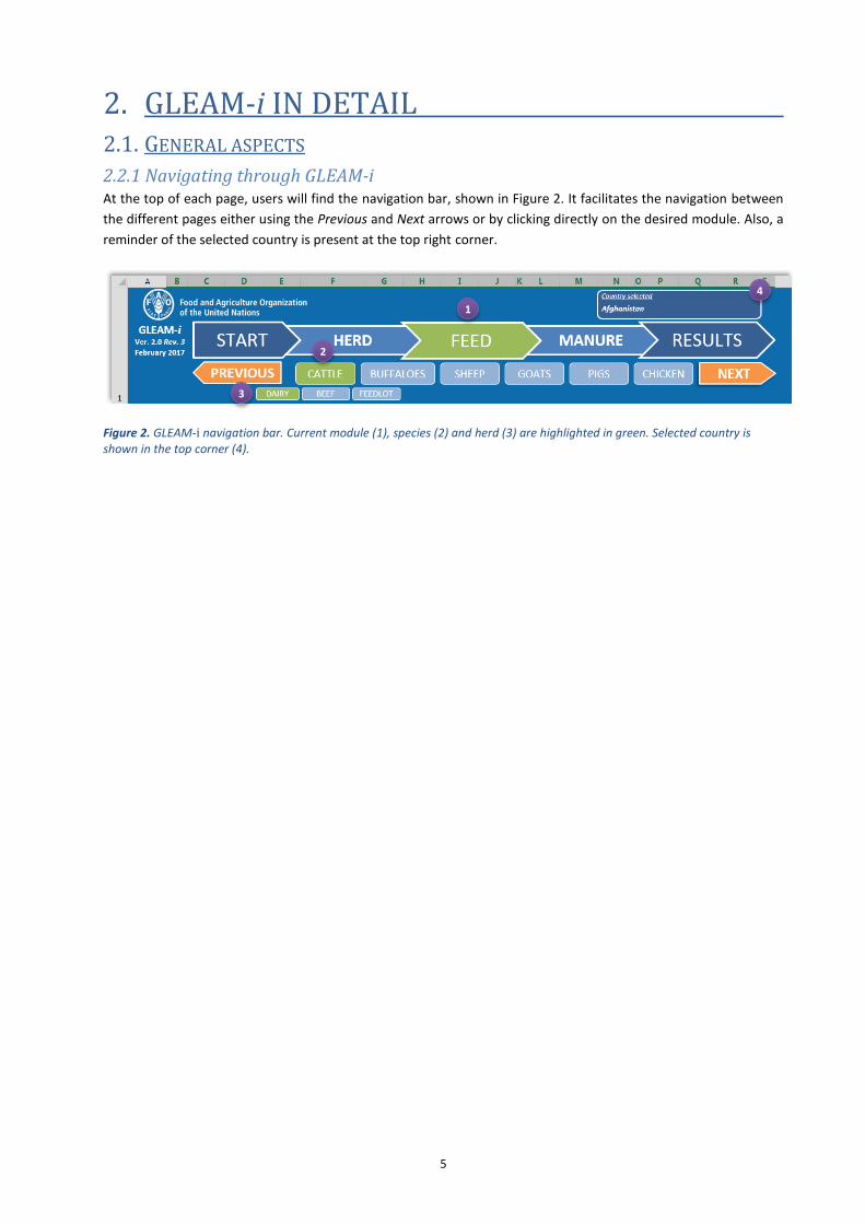
2.2.1 Navigating through GLEAM-i At the top of each page, users will find the navigation bar, shown in Figure 2. It facilitates the navigation between

the different pages either using the Previous and Next arrows or by clicking directly on the desired module. Also, a

reminder of the selected country is present at the top right corner.

Figure 2. GLEAM-i navigation bar. Current module (1), species (2) and herd (3) are highlighted in green. Selected country is shown in the top corner (4).

1

2

3

4

GLEAM-i GLEAM-i IN DETAIL Revision 3 – March 2017

6

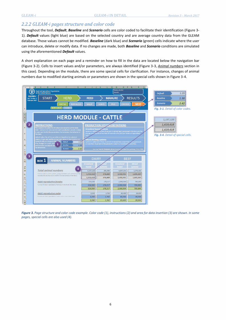
2.2.2 GLEAM-i pages structure and color code Throughout the tool, Default, Baseline and Scenario cells are color coded to facilitate their identification (Figure 3-

1). Default values (light blue) are based on the selected country and are average country data from the GLEAM

database. Those values cannot be modified. Baseline (dark blue) and Scenario (green) cells indicate where the user

can introduce, delete or modify data. If no changes are made, both Baseline and Scenario conditions are simulated

using the aforementioned Default values.

A short explanation on each page and a reminder on how to fill in the data are located below the navigation bar

(Figure 3-2). Cells to insert values and/or parameters, are always identified (Figure 3-3, Animal numbers section in

this case). Depending on the module, there are some special cells for clarification. For instance, changes of animal

numbers due to modified starting animals or parameters are shown in the special cells shown in Figure 3-4.

Figure 3. Page structure and color code example. Color code (1), instructions (2) and area for data insertion (3) are shown. In some pages, special cells are also used (4).

1

2

3

4

Fig. 3-1. Detail of color codes.

Fig. 3-4. Detail of special cells.


7

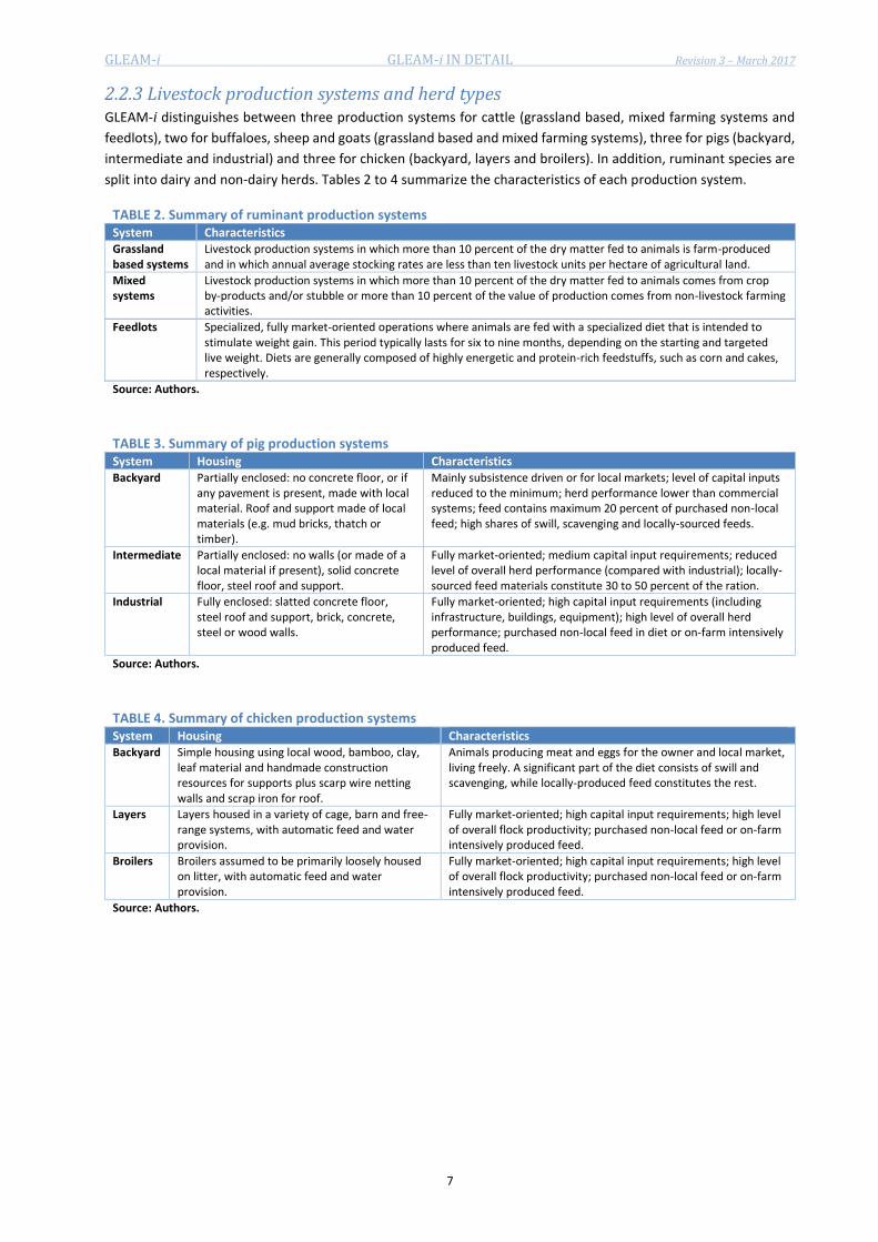
2.2.3 Livestock production systems and herd types GLEAM-i distinguishes between three production systems for cattle (grassland based, mixed farming systems and

feedlots), two for buffaloes, sheep and goats (grassland based and mixed farming systems), three for pigs (backyard,

intermediate and industrial) and three for chicken (backyard, layers and broilers). In addition, ruminant species are

split into dairy and non-dairy herds. Tables 2 to 4 summarize the characteristics of each production system.

TABLE 2. Summary of ruminant production systems System Characteristics Grassland based systems

Livestock production systems in which more than 10 percent of the dry matter fed to animals is farm-produced and in which annual average stocking rates are less than ten livestock units per hectare of agricultural land.

Mixed systems

Livestock production systems in which more than 10 percent of the dry matter fed to animals comes from crop by-products and/or stubble or more than 10 percent of the value of production comes from non-livestock farming activities.

Feedlots Specialized, fully market-oriented operations where animals are fed with a specialized diet that is intended to stimulate weight gain. This period typically lasts for six to nine months, depending on the starting and targeted live weight. Diets are generally composed of highly energetic and protein-rich feedstuffs, such as corn and cakes, respectively.

Source: Authors.

TABLE 3. Summary of pig production systems System Housing Characteristics Backyard Partially enclosed: no concrete floor, or if

any pavement is present, made with local material. Roof and support made of local materials (e.g. mud bricks, thatch or timber).

Mainly subsistence driven or for local markets; level of capital inputs reduced to the minimum; herd performance lower than commercial systems; feed contains maximum 20 percent of purchased non-local feed; high shares of swill, scavenging and locally-sourced feeds.

Intermediate Partially enclosed: no walls (or made of a local material if present), solid concrete floor, steel roof and support.

Fully market-oriented; medium capital input requirements; reduced level of overall herd performance (compared with industrial); locally-sourced feed materials constitute 30 to 50 percent of the ration.

Industrial Fully enclosed: slatted concrete floor, steel roof and support, brick, concrete, steel or wood walls.

Fully market-oriented; high capital input requirements (including infrastructure, buildings, equipment); high level of overall herd performance; purchased non-local feed in diet or on-farm intensively produced feed.

Source: Authors.

TABLE 4. Summary of chicken production systems System Housing Characteristics Backyard Simple housing using local wood, bamboo, clay,

leaf material and handmade construction resources for supports plus scarp wire netting walls and scrap iron for roof.

Animals producing meat and eggs for the owner and local market, living freely. A significant part of the diet consists of swill and scavenging, while locally-produced feed constitutes the rest.

Layers Layers housed in a variety of cage, barn and free-range systems, with automatic feed and water provision.

Fully market-oriented; high capital input requirements; high level of overall flock productivity; purchased non-local feed or on-farm intensively produced feed.

Broilers Broilers assumed to be primarily loosely housed on litter, with automatic feed and water provision.

Fully market-oriented; high capital input requirements; high level of overall flock productivity; purchased non-local feed or on-farm intensively produced feed.

Source: Authors.


8

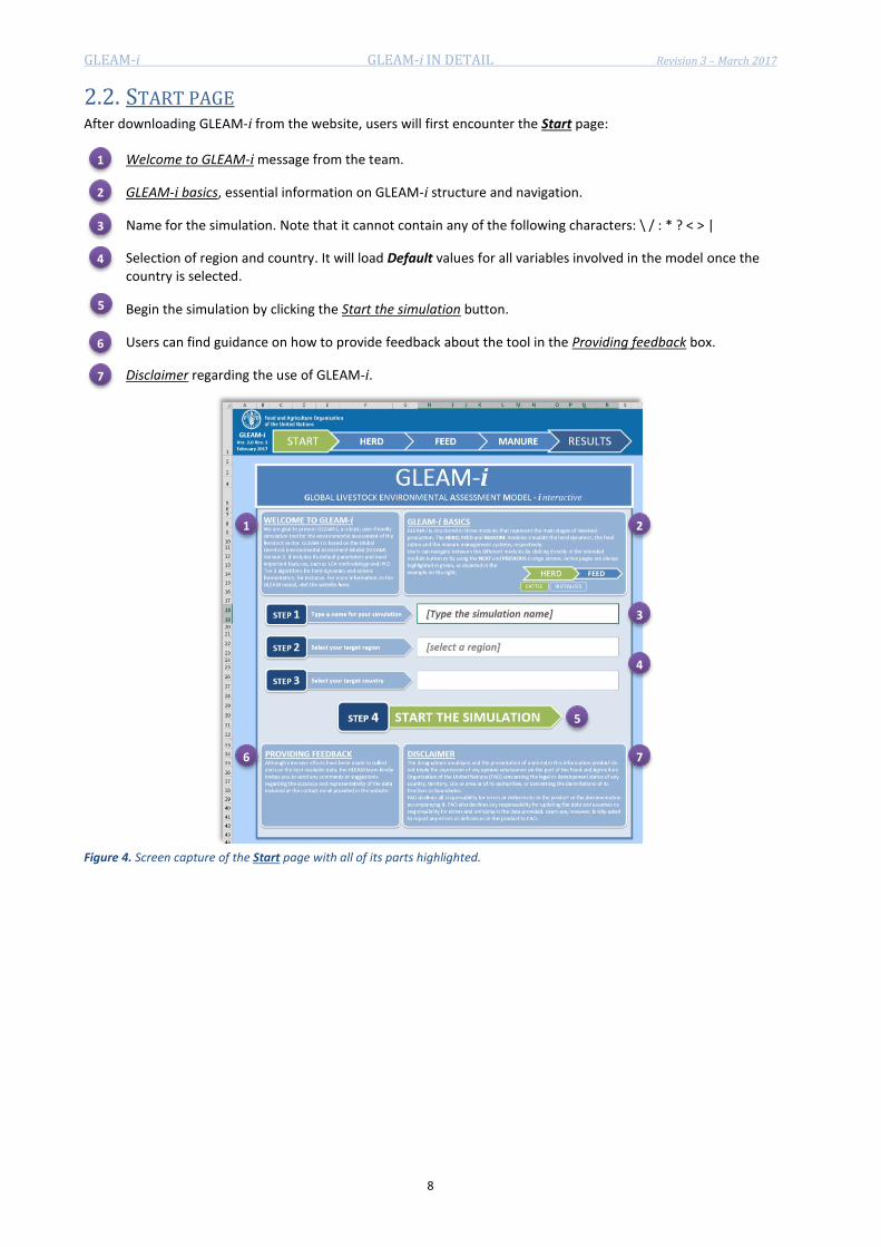
2.2. START PAGE After downloading GLEAM-i from the website, users will first encounter the Start page:

Welcome to GLEAM-i message from the team.

GLEAM-i basics, essential information on GLEAM-i structure and navigation.

Name for the simulation. Note that it cannot contain any of the following characters: \ / : * ? < > |

Selection of region and country. It will load Default values for all variables involved in the model once the country is selected.

Begin the simulation by clicking the Start the simulation button.

Users can find guidance on how to provide feedback about the tool in the Providing feedback box.

Disclaimer regarding the use of GLEAM-i.

Figure 4. Screen capture of the Start page with all of its parts highlighted.

1

2

3

4

5

6

7

1 2

3

4

5

7 6


9

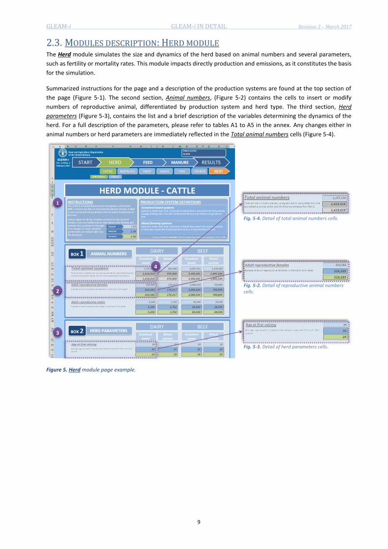
2.3. MODULES DESCRIPTION: HERD MODULE The Herd module simulates the size and dynamics of the herd based on animal numbers and several parameters,

such as fertility or mortality rates. This module impacts directly production and emissions, as it constitutes the basis

for the simulation.

Summarized instructions for the page and a description of the production systems are found at the top section of

the page (Figure 5-1). The second section, Animal numbers, (Figure 5-2) contains the cells to insert or modify

numbers of reproductive animal, differentiated by production system and herd type. The third section, Herd

parameters (Figure 5-3), contains the list and a brief description of the variables determining the dynamics of the

herd. For a full description of the parameters, please refer to tables A1 to A5 in the annex. Any changes either in

animal numbers or herd parameters are immediately reflected in the Total animal numbers cells (Figure 5-4).

Figure 5. Herd module page example.

3

1

2 Fig. 5-2. Detail of reproductive animal numbers cells.

Fig. 5-3. Detail of herd parameters cells.

Fig. 5-4. Detail of total animal numbers cells.

4


10

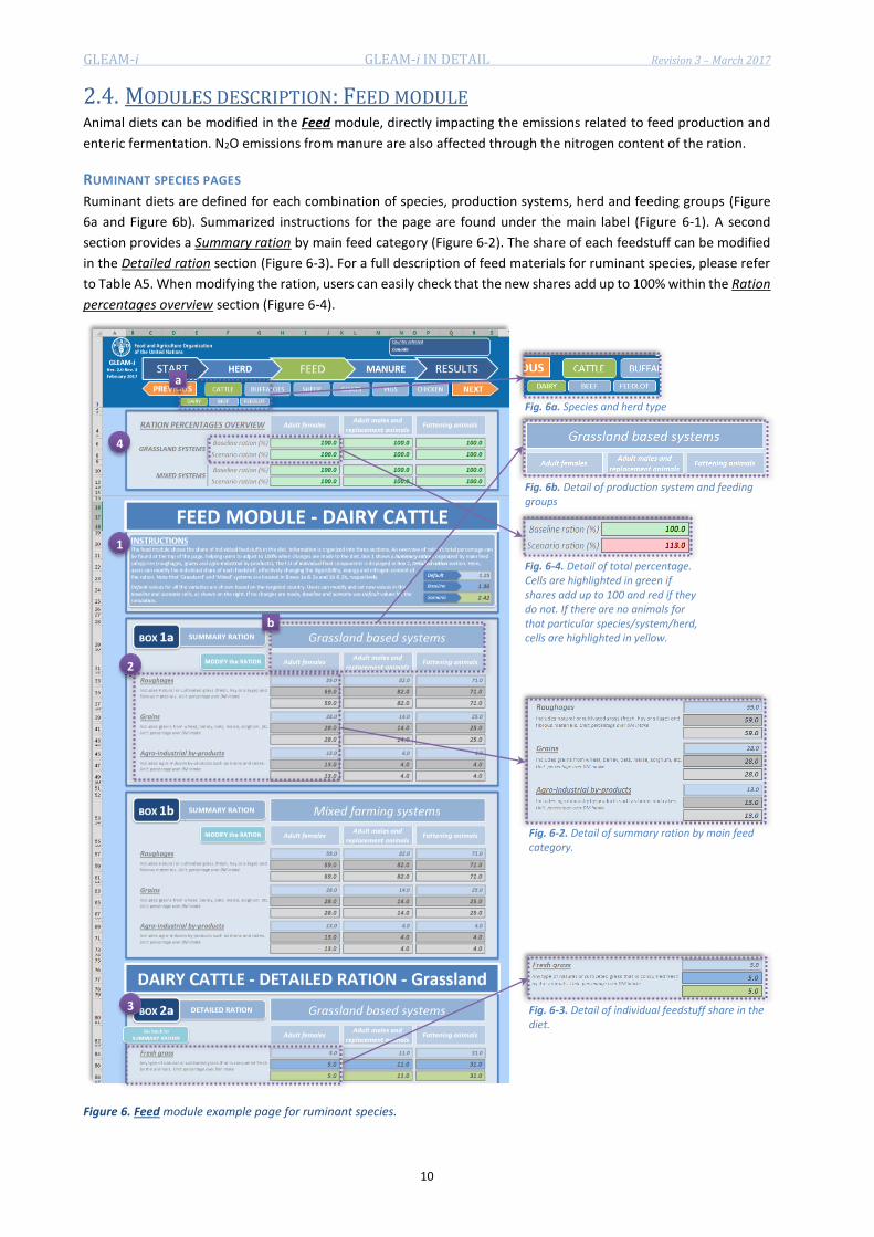
2.4. MODULES DESCRIPTION: FEED MODULE Animal diets can be modified in the Feed module, directly impacting the emissions related to feed production and

enteric fermentation. N2O emissions from manure are also affected through the nitrogen content of the ration.

RUMINANT SPECIES PAGES

Ruminant diets are defined for each combination of species, production systems, herd and feeding groups (Figure

6a and Figure 6b). Summarized instructions for the page are found under the main label (Figure 6-1). A second

section provides a Summary ration by main feed category (Figure 6-2). The share of each feedstuff can be modified

in the Detailed ration section (Figure 6-3). For a full description of feed materials for ruminant species, please refer

to Table A5. When modifying the ration, users can easily check that the new shares add up to 100% within the Ration

percentages overview section (Figure 6-4).

Figure 6. Feed module example page for ruminant species.

4

3

Fig. 6a. Species and herd type

Fig. 6-4. Detail of total percentage. Cells are highlighted in green if shares add up to 100 and red if they do not. If there are no animals for that particular species/system/herd, cells are highlighted in yellow.

Fig. 6b. Detail of production system and feeding groups

Fig. 6-2. Detail of summary ration by main feed category.

Fig. 6-3. Detail of individual feedstuff share in the diet.

a

b

2

1


11

EMISSIONS FROM PASTURE EXPANSION

This page presents the data on emissions arising from the expansion of pastures used for grazing into natural areas.

Following GLEAM, this calculation applies exclusively to specialized beef cattle in grazing systems in the following

countries of Latin America and the Caribbean: Brazil, Chile, Nicaragua, Honduras, Ecuador, Panama, El Salvador and

Belize. For further details on background data and the methodology, please refer to GLEAM model description.

Users can access the page through a dedicated button in the ‘Beef cattle – Grazing systems’ (Figure 7).

Figure 7. Dedicated button in the Beef cattle Feed page to open the Pasture expansion page.

Summarized instructions can be found at the top of the page (Figure 8-1), alongside the result of the calculation

(Figure 8-2). Emissions are calculated using the IPCC Stock-Difference method, which measures carbon stocks at two

points in time to assess carbon changes. Users can modify the length of the period (Figure 8-3) and the area of

expansion (Figure 8-4). Biomass figures depending on the country selection are given for reference (Figure 8-5).

Modifications of Default conditions regarding pasture expansion should be done with additional care, and it is not

recommended to change the given values unless users have a high degree of confidence in the new data.

Figure 8. Pasture expansion page.

1 2

3

4

5


12

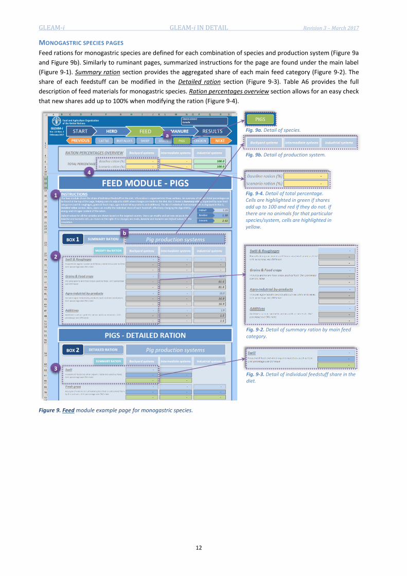
MONOGASTRIC SPECIES PAGES

Feed rations for monogastric species are defined for each combination of species and production system (Figure 9a

and Figure 9b). Similarly to ruminant pages, summarized instructions for the page are found under the main label

(Figure 9-1). Summary ration section provides the aggregated share of each main feed category (Figure 9-2). The

share of each feedstuff can be modified in the Detailed ration section (Figure 9-3). Table A6 provides the full

description of feed materials for monogastric species. Ration percentages overview section allows for an easy check

that new shares add up to 100% when modifying the ration (Figure 9-4).

Figure 9. Feed module example page for monogastric species.

Fig. 9b. Detail of production system.

Fig. 9-2. Detail of summary ration by main feed category.

b

2

3

Fig. 9a. Detail of species.

Fig. 9-4. Detail of total percentage. Cells are highlighted in green if shares add up to 100 and red if they do not. If there are no animals for that particular species/system, cells are highlighted in yellow.

1

Fig. 9-3. Detail of individual feedstuff share in the diet.

a

4


13

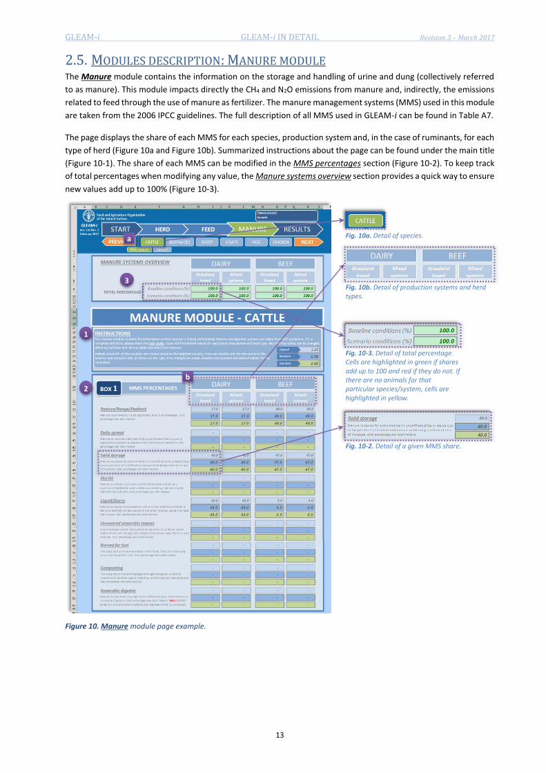
2.5. MODULES DESCRIPTION: MANURE MODULE The Manure module contains the information on the storage and handling of urine and dung (collectively referred

to as manure). This module impacts directly the CH4 and N2O emissions from manure and, indirectly, the emissions

related to feed through the use of manure as fertilizer. The manure management systems (MMS) used in this module

are taken from the 2006 IPCC guidelines. The full description of all MMS used in GLEAM-i can be found in Table A7.

The page displays the share of each MMS for each species, production system and, in the case of ruminants, for each

type of herd (Figure 10a and Figure 10b). Summarized instructions about the page can be found under the main title

(Figure 10-1). The share of each MMS can be modified in the MMS percentages section (Figure 10-2). To keep track

of total percentages when modifying any value, the Manure systems overview section provides a quick way to ensure

new values add up to 100% (Figure 10-3).

Figure 10. Manure module page example.

Fig. 10a. Detail of species. a

b

1

2

3 Fig. 10b. Detail of production systems and herd types.

Fig. 10-3. Detail of total percentage. Cells are highlighted in green if shares add up to 100 and red if they do not. If there are no animals for that particular species/system, cells are highlighted in yellow.

Fig. 10-2. Detail of a given MMS share.


14

2.6. RESULTS PAGES GLEAM-i provides the results of the simulation in two complementary formats. First, a dedicated Results page

contains a series of graphs and figures where Baseline and Scenario conditions are displayed side by side to facilitate

a visual and fast comparison between them. Second, a series of tables with more detailed results by species and

production systems are available for easy numeric comparisons.

At the top of the Results page, users will find the usual navigation bar with a direct access to every module (Figure

11-1). In addition, summary results and detailed tables for each species can be accessed by clicking in their

corresponding buttons (Figure 11-2). Additionally, users can save a copy of all the numeric tables in a separate file

using the Export results button (Figure 11-3). Macros must be enabled to use this feature.

Figure 11. Navigation bar in the Results page.

2.7.1 Graphs – Animal production Estimates on animal production are shown in this section. Graphs include meat production in carcass weight (Figure

12-1), milk production as fresh, raw milk (Figure 12-2) and egg production in shell weight (Figure 12-3). Baseline and

Scenario conditions are represented by blue and green bars, respectively. For Scenario conditions, a label with the

percentage of change respect to the Baseline is also shown to facilitate the comparison (Figure 12-4).

Figure 12. ‘Animal production’ graphs, including meat, milk and eggs production.

1

2 3

1 2 3

4


15

2.7.2 Graphs – Total GHG emissions This section contains the estimates on GHG emissions. First, sector’s total emissions are shown, both numerically

and graphically (Figure 13-1). A second graph shows the share of each gas (CO2, CH4 and N2O) in the aggregated

emissions’ tally (Figure 13-2). The third graphs shows, for each species, the contribution of each emission source

aggregated into four main categories: feed, enteric, manure and energy use. (Figure 13-3). The labels in Scenario

conditions (Figure 13-4) refer to the change of each species’ total emissions.

Figure 13. ‘Greenhouse gas emissions’ graphs, including sector’s total emissions, share by gas and total emissions and main sources by species.

2.7.3 Graphs – Source of emissions The shares and a brief description of all twelve sources included in GLEAM-i are given here, both in the form a

stacked bar graph (Figure 14-1) as well as numeric percentages (Figure 14-2).

Figure 14. ‘Source of emissions’ graphs, were detailed sources for total emissions are shown.

1 2

3

1

2

4


16

2.7.4 Graphs results – GLEAM-i and IPCC Tier 1 The graphs in this section compare the estimated emissions arising from GLEAM-i (Tier 2), and those arising from

IPCC Tier 1 approach. The comparison includes the three sources of emissions from livestock covered in the IPCC

Guidelines (Volume 4, Chapter 10): enteric fermentation and methane and nitrous oxide from manure management.

The graph includes the total of the three for additional reference. Users can find one graph for Baseline (Figure 15-

1) and Scenario conditions (Figure 15-2).

Figure 15. ‘GLEAM-i and IPCC TIER 1’ graphs, showing the comparison between Tier 1 and GLEAM-i estimations of enteric fermentation and manure related emissions.

2.7.5 Graphs results – Emission intensities Emissions related to the production of a given commodity are shown here (Figure 16-1). In order to compare the

environmental performance among different products, meat milk and eggs quantities are converted into edible

protein and production is divided by the emissions associated with their production. Regional average values from

GLEAM are also provided for reference purposes (Figure 16-2).

Figure 16. ‘Emission intensities’ graph, where Baseline and Scenario emission intensities are compared. Regional average values from GLEAM are also provided for reference.

1 2

1 2


17

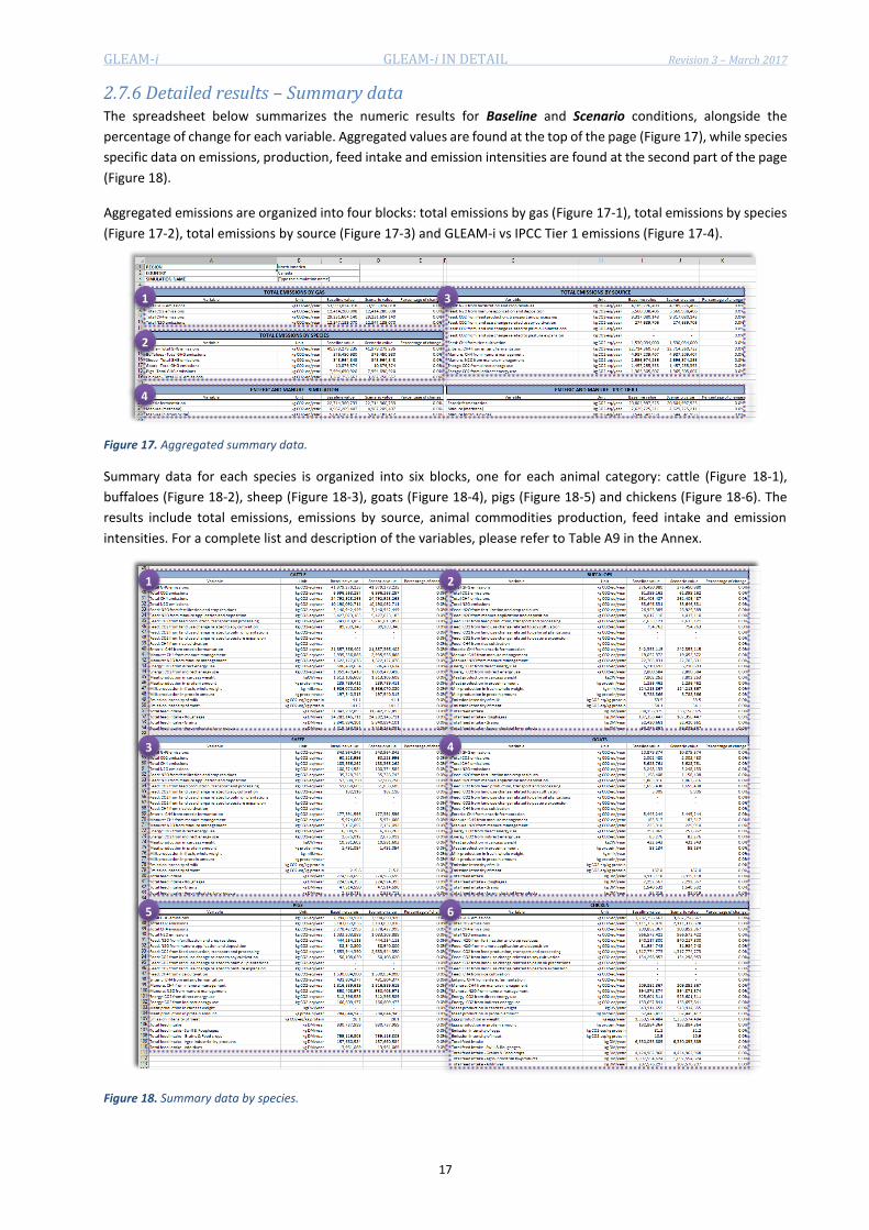
2.7.6 Detailed results – Summary data The spreadsheet below summarizes the numeric results for Baseline and Scenario conditions, alongside the

percentage of change for each variable. Aggregated values are found at the top of the page (Figure 17), while species

specific data on emissions, production, feed intake and emission intensities are found at the second part of the page

(Figure 18).

Aggregated emissions are organized into four blocks: total emissions by gas (Figure 17-1), total emissions by species

(Figure 17-2), total emissions by source (Figure 17-3) and GLEAM-i vs IPCC Tier 1 emissions (Figure 17-4).

Figure 17. Aggregated summary data.

Summary data for each species is organized into six blocks, one for each animal category: cattle (Figure 18-1),

buffaloes (Figure 18-2), sheep (Figure 18-3), goats (Figure 18-4), pigs (Figure 18-5) and chickens (Figure 18-6). The

results include total emissions, emissions by source, animal commodities production, feed intake and emission

intensities. For a complete list and description of the variables, please refer to Table A9 in the Annex.

Figure 18. Summary data by species.

1

2

3

4

1

3 4

5 6

2


18

2.7.7 Detailed results – Ruminant species Detailed, disaggregated data for ruminant species are displayed in this page (Figure 19). Users can filter the results

by species, production system, herd type and variable (Figure 19-1). The page presents results on total emissions,

emission sources, production, animal numbers, feed intake and emission intensities. Table A9 contains the full list

and description of all the variables.

Figure 19. Detailed data spreadsheet for ruminant species.

2.7.8 Detailed results – Monogastric species Detailed, disaggregated data on monogastrics can be found in the dedicated spreadsheets for pigs and chickens.

Similarly to ruminants, data can be filtered by species, production systems and variable (Figure 20-1). The page

presents results on total emissions, emission sources, production, animal numbers, feed intake and emission

intensities. Table A9 contains the full list and description of all the variables.

Figure 20. Example of detailed data spreadsheet for monogastric species.

1

Fig. 19-1. Detail of available filters in detailed results pages.

1 Fig. 20-1. Detail of available filters in detailed results pages.

19

3. STEP-BY-STEP EXAMPLE ________________________ This chapter provides a practical example on how to run a simulation that involves setting a Baseline and

implementing a Scenario that consists of several intervention measures in all modules.

3.1. SETTING THE BASELINE The first step to assess the impact of any intervention measures is to establish and characterize the starting

conditions. When defining the Baseline, users should consider two possibilities:

- Case 1. If users do not have complete and/or reliable information regarding any of the parameters and

values required to run the simulation, Baseline conditions should make use of the Default values provided

by the tool.

- Case 2. Otherwise, users should modify any value or parameter for which sufficient and reliable information

is available, setting more realistic Baseline conditions.

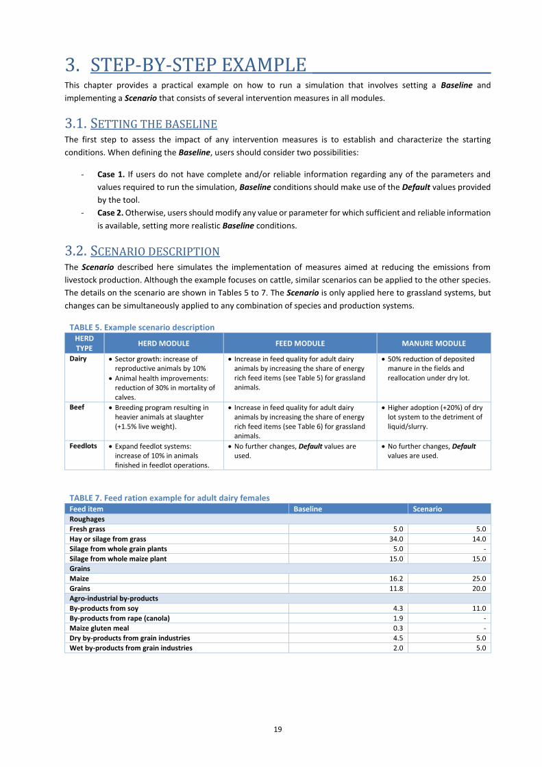
3.2. SCENARIO DESCRIPTION The Scenario described here simulates the implementation of measures aimed at reducing the emissions from

livestock production. Although the example focuses on cattle, similar scenarios can be applied to the other species.

The details on the scenario are shown in Tables 5 to 7. The Scenario is only applied here to grassland systems, but

changes can be simultaneously applied to any combination of species and production systems.

TABLE 5. Example scenario description HERD TYPE

HERD MODULE FEED MODULE MANURE MODULE

Dairy Sector growth: increase of reproductive animals by 10%

Animal health improvements: reduction of 30% in mortality of calves.

Increase in feed quality for adult dairy animals by increasing the share of energy rich feed items (see Table 5) for grassland animals.

50% reduction of deposited manure in the fields and reallocation under dry lot.

Beef Breeding program resulting in heavier animals at slaughter (+1.5% live weight).

Increase in feed quality for adult dairy animals by increasing the share of energy rich feed items (see Table 6) for grassland animals.

Higher adoption (+20%) of dry lot system to the detriment of liquid/slurry.

Feedlots Expand feedlot systems: increase of 10% in animals finished in feedlot operations.

No further changes, Default values are used.

No further changes, Default values are used.

TABLE 7. Feed ration example for adult dairy females Feed item Baseline Scenario Roughages

Fresh grass 5.0 5.0

Hay or silage from grass 34.0 14.0

Silage from whole grain plants 5.0 -

Silage from whole maize plant 15.0 15.0

Grains

Maize 16.2 25.0

Grains 11.8 20.0

Agro-industrial by-products

By-products from soy 4.3 11.0

By-products from rape (canola) 1.9 -

Maize gluten meal 0.3 -

Dry by-products from grain industries 4.5 5.0

Wet by-products from grain industries 2.0 5.0

GLEAM-i STEP-BY-STEP EXAMPLE Revision 3 – March 2017

20

TABLE 8. Feed ration example for fattening beef animals Feed item Baseline Scenario Roughages

Fresh grass 46.0 20.0

Hay or silage from grass 24.0 15.0

Silage from whole grain plants 8.0 5.0

Silage from whole maize plant 8.0 -

Grains

Maize 5.0 20.0

Grains 5.0 15.0


By-products from soy 1.0 10.0

By-products from rape (canola) 1.0 5.0

Dry by-products from grain industries 1.0 5.0

Wet by-products from grain industries 1.0 5.0


21

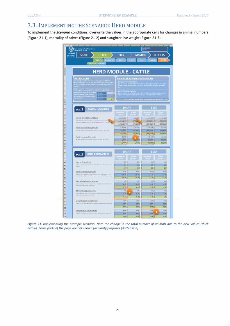
3.3. IMPLEMENTING THE SCENARIO: HERD MODULE To implement the Scenario conditions, overwrite the values in the appropriate cells for changes in animal numbers

(Figure 21-1), mortality of calves (Figure 21-2) and slaughter live weight (Figure 21-3).

Figure 21. Implementing the example scenario. Note the change in the total number of animals due to the new values (thick arrow). Some parts of the page are not shown for clarity purposes (dotted line).

1

2

3


22

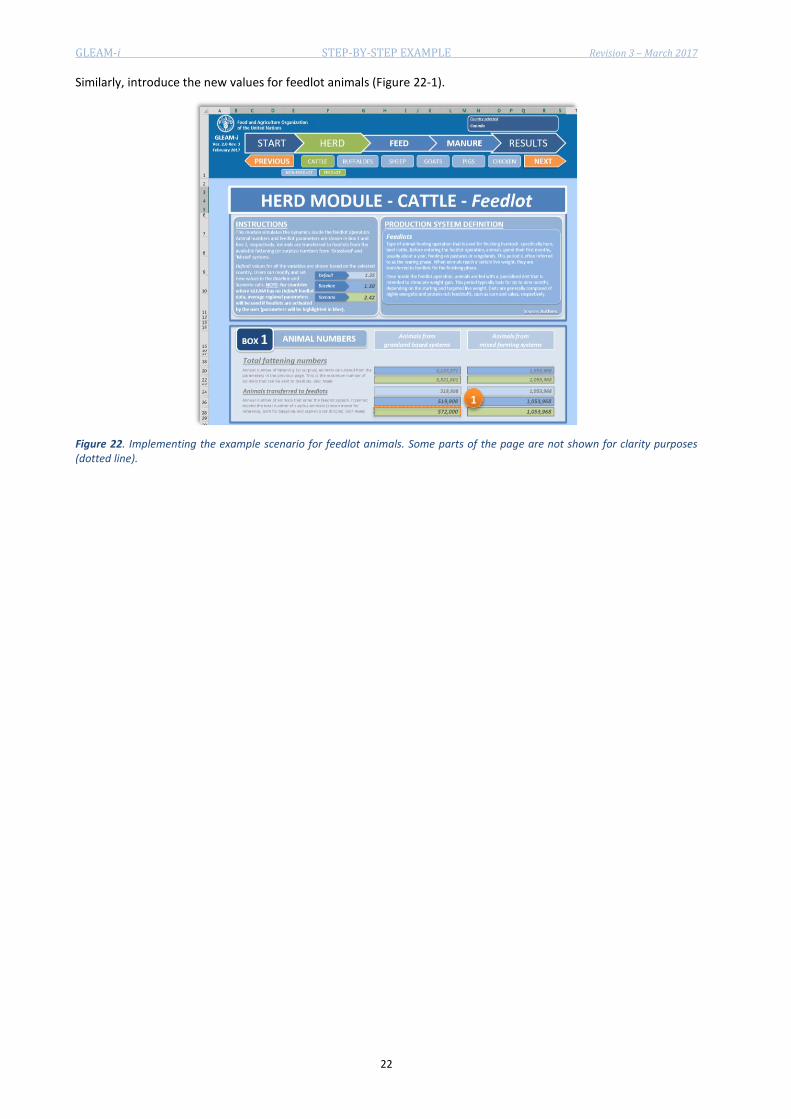
Similarly, introduce the new values for feedlot animals (Figure 22-1).

Figure 22. Implementing the example scenario for feedlot animals. Some parts of the page are not shown for clarity purposes (dotted line).

1


23

3.4. IMPLEMENTING THE SCENARIO: FEED MODULE

3.4.1 Implementing the scenario – Feed module for dairy animals Introduce the new values in the Scenario cells according to the diet defined in Table 6 (Figure 23-1). Check that the

total percentage adds up to 100% for the new conditions (Figure 23-2).

Figure 23. Implementing the example scenario. Some parts of the page are not shown for clarity purposes (dotted line).

1

2


24

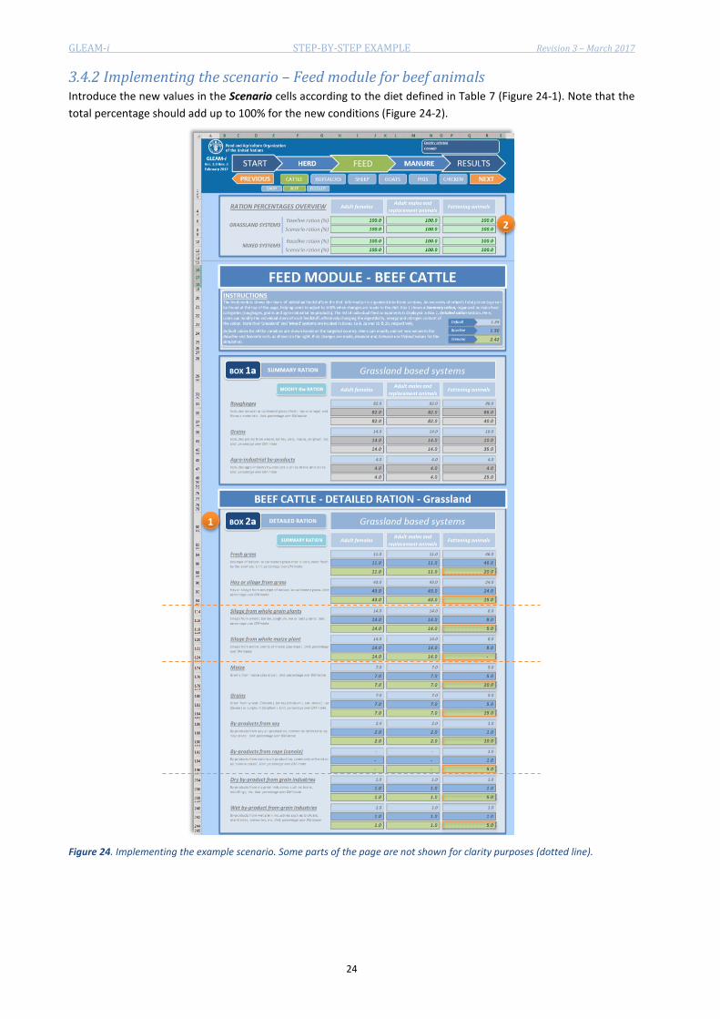
3.4.2 Implementing the scenario – Feed module for beef animals Introduce the new values in the Scenario cells according to the diet defined in Table 7 (Figure 24-1). Note that the

total percentage should add up to 100% for the new conditions (Figure 24-2).

Figure 24. Implementing the example scenario. Some parts of the page are not shown for clarity purposes (dotted line).

1

2


25

3.5. IMPLEMENTING THE SCENARIO: MANURE MODULE To implement the Scenario conditions, overwrite the values in the appropriate cells for each manure management

system for both dairy animals (Figure 25-1) and beef animals (Figure 25-2).

Figure 25. Implementing the example scenario. When modifying the share of manure management systems, make sure they add up to 100%, as shown in the Manure systems overview box.

1 2


26

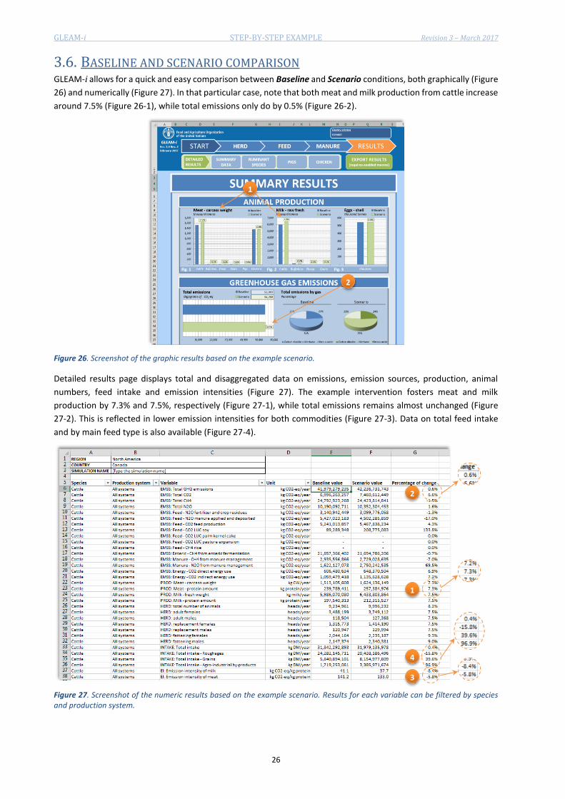
3.6. BASELINE AND SCENARIO COMPARISON GLEAM-i allows for a quick and easy comparison between Baseline and Scenario conditions, both graphically (Figure

26) and numerically (Figure 27). In that particular case, note that both meat and milk production from cattle increase

around 7.5% (Figure 26-1), while total emissions only do by 0.5% (Figure 26-2).

Figure 26. Screenshot of the graphic results based on the example scenario.

Detailed results page displays total and disaggregated data on emissions, emission sources, production, animal

numbers, feed intake and emission intensities (Figure 27). The example intervention fosters meat and milk

production by 7.3% and 7.5%, respectively (Figure 27-1), while total emissions remains almost unchanged (Figure

27-2). This is reflected in lower emission intensities for both commodities (Figure 27-3). Data on total feed intake

and by main feed type is also available (Figure 27-4).

Figure 27. Screenshot of the numeric results based on the example scenario. Results for each variable can be filtered by species and production system.

1

2

1

2

3

4


27

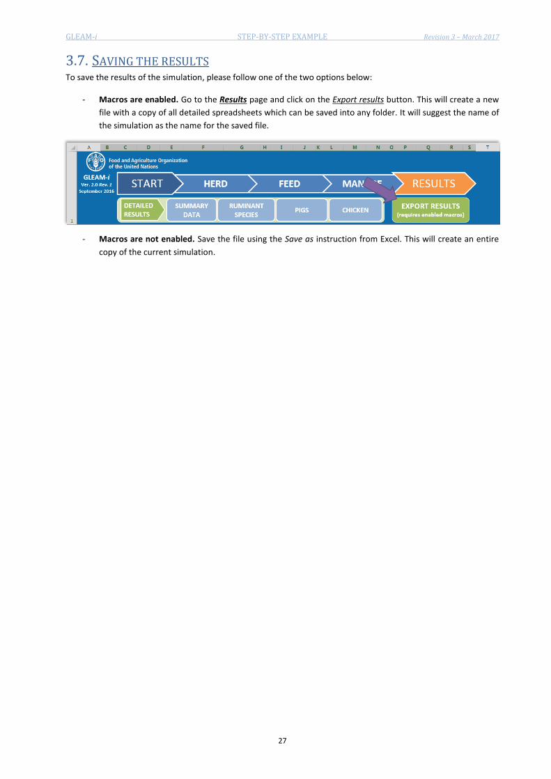
3.7. SAVING THE RESULTS To save the results of the simulation, please follow one of the two options below:

- Macros are enabled. Go to the Results page and click on the Export results button. This will create a new

file with a copy of all detailed spreadsheets which can be saved into any folder. It will suggest the name of

the simulation as the name for the saved file.

- Macros are not enabled. Save the file using the Save as instruction from Excel. This will create an entire

copy of the current simulation.

28

4. ANNEX _____________________________________________ This Annex presents the list and description of all parameters used in GLEAM-i.

TABLE A1. HERD module – Herd parameters: cattle and buffaloes Parameter Description Unit Age at first calving Average age at which cows have their first parturition, either it is a successful one or not. Months

Fertility of adult females

Average fertility rate, expressed as the percentage of calving adult cows over the total amount of adult cows. This includes born calves that die before reaching maturity.

Percentage

Mortality of young females

Annual average percentage of non-intended deaths of female animals before reaching maturity.

Percentage

Mortality of young males

Annual average percentage of non-intended deaths of male animals before reaching maturity. Percentage

Mortality of adult animals

Annual average percentage of non-intended deaths of animals (males and females), after reaching maturity.

Percentage

Adult females replacement

Annual average percentage of adult females’ replacement. Percentage

Weight at birth Average live weight of calves at birth. Kilograms/animal

Weight of adult females

Average live weight of cows once they reach maturity. Kilograms/animal

Weight of adult males

Average live weight of bulls once they reach maturity. Kilograms/animal

Weight of fattening females

Average live weight at slaughter of adult females culled for meat. Kilograms/animal

Weight of fattening males

Average live weight at slaughter of adult males culled for meat. Kilograms/animal

Milk yield Annual average milk yield per milking cow. Kilograms/animal

Milk fat Average milk total fat content. Percentage

Milk protein Average milk total protein content. Percentage

TABLE A2. HERD module – Herd parameters: feedlot operations

Parameter Description Unit Initial weight – Female animals Average live weight of female animals when are transferred to feedlot

operations Kilograms/animal

Weight at slaughter – Female animals

Average live weight at which feedlot female animals are slaughtered Kilograms/animal

Initial weight – Male animals Average live weight of male animals when are transferred to feedlot operations

Kilograms/animal

Weight at slaughter – Male animals Average live weight at which feedlot male animals are slaughtered Kilograms/animal

Finishing period Average duration of the finishing period Days

TABLE A3. HERD module – Herd parameters: sheep and goats

Parameter Description Unit Age at first calving Average age at which does/ewes have their first parturition, either it is a successful one or not. Months

Fertility of adult females

Average fertility rate, expressed as the percentage of lambing (or kidding) adult ewes (or does) over the total amount of adult ewes (or does). This includes born lambs/kids that die before reaching maturity.

Percentage

Parturition interval Average interval between two consecutive parturitions. Days

Litter size Average number of lambs/kids born in each parturition, including those that die before reaching maturity.

Number

Mortality of young animals

Annual average percentage of non-intended deaths of animals before they reach maturity. Percentage

Mortality of adult animals

Annual average percentage of non-intended deaths of adult animals after reaching maturity. Percentage

Adult females replacement

Annual average percentage of adult females’ replacement. Percentage

Weight at birth Average live weight of lambs/kids at birth. Kilograms/animal

Weight of adult females

Average live weight of does/ewes once they reach maturity. Kilograms/animal

Weight of adult males

Average live weight of rams/bucks once they reach maturity. Kilograms/animal

Weight of fattening females

Average live weight at slaughter of adult females culled for meat. Kilograms/animal

Weight of fattening males

Average live weight at slaughter of adult males culled for meat. Kilograms/animal

Milk yield Annual average milk yield per milking doe/ewe. Kilograms/animal

Milk fat Average milk total fat content. Percentage

Milk protein Average milk total protein content. Percentage

GLEAM-i ANNEX Revision 3 – March 2017

29

TABLE A4. HERD module – Herd parameters: pigs

Parameter Description Unit Age at first parturition Average age at which sows have their first parturition, either it is a successful

one or not. Weeks

Fertility of adult females Annual average of parturitions per sows, including all the sows in the herd. Number/animal

Gestation period Average duration of the gestation period. Days

Litter size Average number of piglets born in each parturition, including those that die before reaching maturity.

Number

Lactation period Average amount of time that piglets are lactated. Days

Idle period Average amount of time between one parturition and the consecutive pregnancy.

Days

Mortality of piglets before weaning

Annual average mortality of non-intended piglets’ deaths before weaning. Percentage

Weaning age Average age at which piglets are weaned. Days

Mortality of juvenile replacement animals

Annual average mortality of replacement animals with ages comprised between weaning and maturity.

Percentage

Mortality of adult replacement animals

Annual average mortality of replacement animals after reaching maturity. Percentage

Mortality of fattening animals Annual average mortality of adult fattening animals. Percentage

Replacement of adult females Rate of reproductive adult females’ replacement. Percentage

Replacement of adult males Rate of reproductive adult males’ replacement. Percentage

Weight of piglets at birth Average live weight of piglets at birth. Kilograms/animal

Weight of weaned piglets Average live weight of piglets at weaning age Kilograms/animal

Weight of adult females Average live weight of sows once they reach maturity. Kilograms/animal

Weight of adult males Average live weight of boars once they reach maturity. Kilograms/animal

Weight of fattening animals Average live weight at slaughter of fattening animals culled for meat. Kilograms/animal

Average daily weight gain Average daily weight gain of fattening animals. Kilograms/animal/day

Source: Authors

TABLE A5. HERD module – Herd parameters: chicken

Parameter Description Unit Laying age Average age at which hens starts laying eggs. Weeks

Annual laid eggs Annual average number of eggs laid per hen. Eggs/animal

Hatchability Average percentage of successfully hatched eggs. Percentage

Mortality of pullets Annual average percentage of non-intended deaths of pullets under 16 weeks old.

Percentage

Mortality of adult animals Annual average percentage of non-intended deaths of pullets after their first 16 weeks

Percentage

Egg weight Average weight of eggs Grams/egg

Weight of pullets at birth Average live weight of pullets at hatching Grams/animal

Slaughter weight of backyard hens Average live weight of hens when slaughter for meat in backyard production system

Kilograms/animal

Slaughter weight of backyard roosters

Average live weight of roosters when slaughter for meat in backyard production system

Kilograms/animal

Molting Is molting done in laying systems? Boolean

Initial weight of laying hens Average live weight of laying hens at the beginning of the first laying period Kilograms/animal

Final weight of laying hens Average live weight of laying hens at the end of the first laying period Kilograms/animal

Laying period Average length of the laying period for hens in layer and broiler systems Days

Mortality of adult broilers Average percentage of non-intended deaths of broiler animals after their first 16 weeks

Percentage

Slaughter weight of broilers Average live weight at slaughter of broiler animals Kilograms/animal

Source: Authors


30

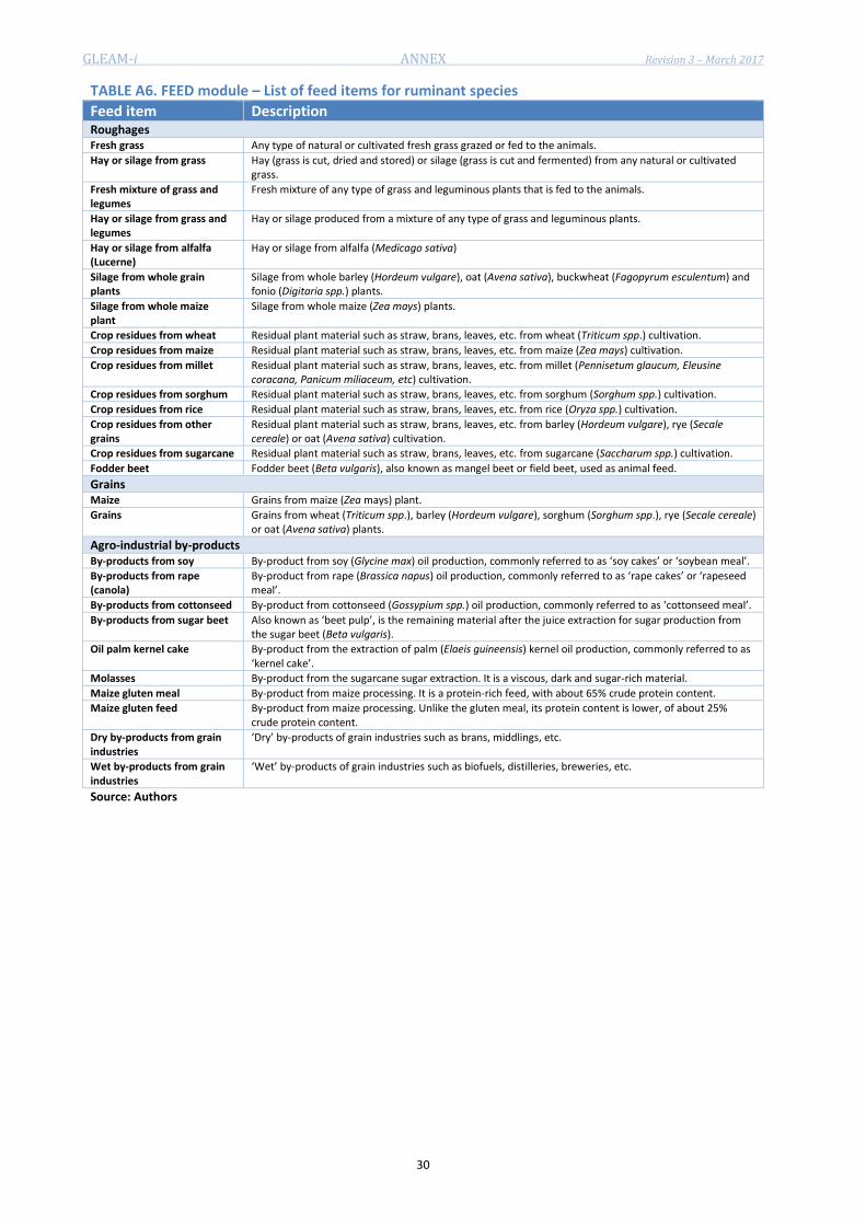
TABLE A6. FEED module – List of feed items for ruminant species

Feed item Description Roughages

Fresh grass Any type of natural or cultivated fresh grass grazed or fed to the animals.

Hay or silage from grass Hay (grass is cut, dried and stored) or silage (grass is cut and fermented) from any natural or cultivated grass.

Fresh mixture of grass and legumes

Fresh mixture of any type of grass and leguminous plants that is fed to the animals.

Hay or silage from grass and legumes

Hay or silage produced from a mixture of any type of grass and leguminous plants.

Hay or silage from alfalfa (Lucerne)

Hay or silage from alfalfa (Medicago sativa)

Silage from whole grain plants

Silage from whole barley (Hordeum vulgare), oat (Avena sativa), buckwheat (Fagopyrum esculentum) and fonio (Digitaria spp.) plants.

Silage from whole maize plant

Silage from whole maize (Zea mays) plants.

Crop residues from wheat Residual plant material such as straw, brans, leaves, etc. from wheat (Triticum spp.) cultivation.

Crop residues from maize Residual plant material such as straw, brans, leaves, etc. from maize (Zea mays) cultivation.

Crop residues from millet Residual plant material such as straw, brans, leaves, etc. from millet (Pennisetum glaucum, Eleusine coracana, Panicum miliaceum, etc) cultivation.

Crop residues from sorghum Residual plant material such as straw, brans, leaves, etc. from sorghum (Sorghum spp.) cultivation.

Crop residues from rice Residual plant material such as straw, brans, leaves, etc. from rice (Oryza spp.) cultivation.

Crop residues from other grains

Residual plant material such as straw, brans, leaves, etc. from barley (Hordeum vulgare), rye (Secale cereale) or oat (Avena sativa) cultivation.

Crop residues from sugarcane Residual plant material such as straw, brans, leaves, etc. from sugarcane (Saccharum spp.) cultivation.

Fodder beet Fodder beet (Beta vulgaris), also known as mangel beet or field beet, used as animal feed.

Grains

Maize Grains from maize (Zea mays) plant.

Grains Grains from wheat (Triticum spp.), barley (Hordeum vulgare), sorghum (Sorghum spp.), rye (Secale cereale) or oat (Avena sativa) plants.

Agro-industrial by-products By-products from soy By-product from soy (Glycine max) oil production, commonly referred to as ‘soy cakes’ or ‘soybean meal’.

By-products from rape (canola)

By-product from rape (Brassica napus) oil production, commonly referred to as ‘rape cakes’ or ‘rapeseed meal’.

By-products from cottonseed By-product from cottonseed (Gossypium spp.) oil production, commonly referred to as ‘cottonseed meal’.

By-products from sugar beet Also known as ‘beet pulp’, is the remaining material after the juice extraction for sugar production from the sugar beet (Beta vulgaris).

Oil palm kernel cake By-product from the extraction of palm (Elaeis guineensis) kernel oil production, commonly referred to as ‘kernel cake’.

Molasses By-product from the sugarcane sugar extraction. It is a viscous, dark and sugar-rich material.

Maize gluten meal By-product from maize processing. It is a protein-rich feed, with about 65% crude protein content.

Maize gluten feed By-product from maize processing. Unlike the gluten meal, its protein content is lower, of about 25% crude protein content.

Dry by-products from grain industries

‘Dry’ by-products of grain industries such as brans, middlings, etc.

Wet by-products from grain industries

‘Wet’ by-products of grain industries such as biofuels, distilleries, breweries, etc.

Source: Authors


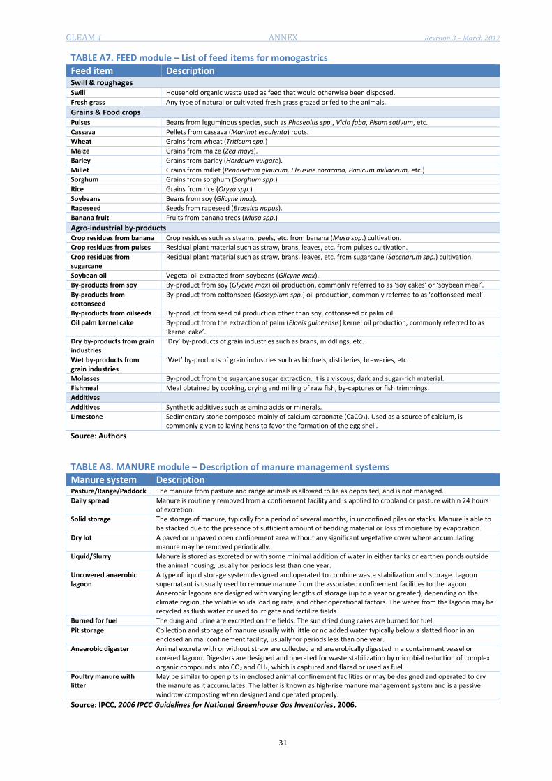
31

TABLE A7. FEED module – List of feed items for monogastrics

Feed item Description Swill & roughages

Swill Household organic waste used as feed that would otherwise been disposed.

Fresh grass Any type of natural or cultivated fresh grass grazed or fed to the animals.

Grains & Food crops

Pulses Beans from leguminous species, such as Phaseolus spp., Vicia faba, Pisum sativum, etc.

Cassava Pellets from cassava (Manihot esculenta) roots.

Wheat Grains from wheat (Triticum spp.)

Maize Grains from maize (Zea mays).

Barley Grains from barley (Hordeum vulgare).

Millet Grains from millet (Pennisetum glaucum, Eleusine coracana, Panicum miliaceum, etc.)

Sorghum Grains from sorghum (Sorghum spp.)

Rice Grains from rice (Oryza spp.)

Soybeans Beans from soy (Glicyne max).

Rapeseed Seeds from rapeseed (Brassica napus).

Banana fruit Fruits from banana trees (Musa spp.)


Crop residues from banana Crop residues such as steams, peels, etc. from banana (Musa spp.) cultivation.

Crop residues from pulses Residual plant material such as straw, brans, leaves, etc. from pulses cultivation.

Crop residues from sugarcane

Residual plant material such as straw, brans, leaves, etc. from sugarcane (Saccharum spp.) cultivation.

Soybean oil Vegetal oil extracted from soybeans (Glicyne max).

By-products from soy By-product from soy (Glycine max) oil production, commonly referred to as ‘soy cakes’ or ‘soybean meal’.

By-products from cottonseed

By-product from cottonseed (Gossypium spp.) oil production, commonly referred to as ‘cottonseed meal’.

By-products from oilseeds By-product from seed oil production other than soy, cottonseed or palm oil.

Oil palm kernel cake By-product from the extraction of palm (Elaeis guineensis) kernel oil production, commonly referred to as ‘kernel cake’.

Dry by-products from grain industries

‘Dry’ by-products of grain industries such as brans, middlings, etc.

Wet by-products from grain industries

‘Wet’ by-products of grain industries such as biofuels, distilleries, breweries, etc.

Molasses By-product from the sugarcane sugar extraction. It is a viscous, dark and sugar-rich material.

Fishmeal Meal obtained by cooking, drying and milling of raw fish, by-captures or fish trimmings.

Additives

Additives Synthetic additives such as amino acids or minerals.

Limestone Sedimentary stone composed mainly of calcium carbonate (CaCO3). Used as a source of calcium, is commonly given to laying hens to favor the formation of the egg shell.

Source: Authors

TABLE A8. MANURE module – Description of manure management systems

Manure system Description Pasture/Range/Paddock The manure from pasture and range animals is allowed to lie as deposited, and is not managed.

Daily spread Manure is routinely removed from a confinement facility and is applied to cropland or pasture within 24 hours of excretion.

Solid storage The storage of manure, typically for a period of several months, in unconfined piles or stacks. Manure is able to be stacked due to the presence of sufficient amount of bedding material or loss of moisture by evaporation.

Dry lot A paved or unpaved open confinement area without any significant vegetative cover where accumulating manure may be removed periodically.

Liquid/Slurry Manure is stored as excreted or with some minimal addition of water in either tanks or earthen ponds outside the animal housing, usually for periods less than one year.

Uncovered anaerobic lagoon

A type of liquid storage system designed and operated to combine waste stabilization and storage. Lagoon supernatant is usually used to remove manure from the associated confinement facilities to the lagoon. Anaerobic lagoons are designed with varying lengths of storage (up to a year or greater), depending on the climate region, the volatile solids loading rate, and other operational factors. The water from the lagoon may be recycled as flush water or used to irrigate and fertilize fields.

Burned for fuel The dung and urine are excreted on the fields. The sun dried dung cakes are burned for fuel.

Pit storage Collection and storage of manure usually with little or no added water typically below a slatted floor in an enclosed animal confinement facility, usually for periods less than one year.

Anaerobic digester Animal excreta with or without straw are collected and anaerobically digested in a containment vessel or covered lagoon. Digesters are designed and operated for waste stabilization by microbial reduction of complex organic compounds into CO2 and CH4, which is captured and flared or used as fuel.

Poultry manure with litter

May be similar to open pits in enclosed animal confinement facilities or may be designed and operated to dry the manure as it accumulates. The latter is known as high-rise manure management system and is a passive windrow composting when designed and operated properly.

Source: IPCC, 2006 IPCC Guidelines for National Greenhouse Gas Inventories, 2006.


32

TABLE A9. DETAILED RESULTS page – Description of variables

Variable Description EMSS: Total GHG emissions Total GHG emissions.

EMSS: Total CO2 Total carbon dioxide emissions.

EMSS: Total CH4 Total methane emissions.

EMSS: Total N2O Total nitrous oxide emissions.

EMSS: Feed - N2O fertilizer and crop residues

N2O emissions from the conversion of nitrogenous compounds present in synthetic nitrogenous fertilizers applied to feed crops and from the decomposition of crop residues. It includes direct emissions (conversions of nitrogen into N2O through a combination of nitrification and denitrification processes) and indirect emissions (nitrogen is lost in forms of ammonia and NOx).

EMSS: Feed - N2O manure applied and deposited

N2O emissions from the conversion of nitrogenous compounds present in animal excreta: manure can be deposited in the fields by grazing and scavenging animals or applied to feed crop fields as organic fertilizer. It includes direct emissions (conversions of nitrogen into N2O through a combination of nitrification and denitrification processes) and indirect emissions (nitrogen is lost in forms of ammonia and NOx).

EMSS: Feed - CO2 feed production CO2 emissions arising from the production, transport and processing of feed. This includes emissions from fossil fuels use in fertilizer and pesticides manufacture, field operations and feed manufacture in feed mills.

EMSS: Feed - CO2 LUC soy CO2 emissions due to the expansion of soybean cultivation into natural areas. Emissions are related to changes in carbon stored in biomass, dead organic matter and soils.

EMSS: Feed - CO2 LUC palm kernel cake

CO2 emissions due to the expansion of palm oil plantations into natural areas. Emissions are related to changes in carbon stored in biomass, dead organic matter and soils.

EMSS: Feed - CO2 LUC pasture expansion

CO2 emissions due to the expansion of pastures into natural areas. Emissions are related to changes in carbon stored in biomass, dead organic matter and soils.

EMSS: Feed - CH4 rice CH4 emissions from the cultivation of rice used as feed. Emissions are related to anaerobic decomposition of organic matter in flooded rice fields.

EMSS: Enteric - CH4 from enteric fermentation

CH4 emissions from enteric fermentation of ruminant species and pigs. During the digestive process, microbial fermentation breaks down part of the carbohydrates in the diet, generating methane as a by-product. In general, fibrous materials cause higher enteric emissions.

EMSS: Manure - CH4 from manure management

CH4 emissions from the anaerobic decomposition of organic material present in animal excreta. This is most common when urine and dung are stored and treated in liquid-based systems.

EMSS: Manure - N2O from manure management

N2O emissions from the conversion of nitrogenous compounds present in animal excreta. It includes direct emissions (conversions of nitrogen into N2O through a combination of nitrification and denitrification processes) and indirect emissions (nitrogen is lost in forms of ammonia and NOx).

EMSS: Energy - CO2 direct energy use CO2 emissions from the use of energy in the animal production site for heating, ventilation, refrigeration, machinery, etc.

EMSS: Energy - CO2 indirect energy use CO2 emissions from the use of energy on the construction of facilities (animal housing) and equipment.

PROD: Meat - carcass weight Total production of meat expressed in carcass weight

PROD: Meat - protein amount Total production of meat expressed in protein amount

PROD: Milk - fresh weight Total production of milk expressed in whole, fresh weight

PROD: Milk - protein amount Total production of milk expressed in protein amount

PROD: Eggs - shell weight Total production of eggs expressed in whole, shell weight

PROD: Eggs - protein amount Total production of eggs expressed in protein amount

HERD: total number of animals Total number of animal heads. It includes all cohorts for a given species. Applies to all species.

HERD: adult females Total number of adult female animals for a given species. Applies to all species.

HERD: adult males Total number of adult male animals for a given species. Applies to all species.

HERD: replacement females Total number of replacement female animals for a given species. Applies to all species.

HERD: replacement males Total number of replacement male animals for a given species. Applies to all species.

HERD: fattening females Total number of surplus female animals for a given species. Applies to ruminant species and chicken.

HERD: fattening males Total number of surplus male animals for a given species. Applies to ruminant species and chicken.

HERD: fattening animals Total number of surplus animals. Applies to pigs and chicken only.

INTAKE: Total intake Total annual dry matter intake by the herd (or flock) of a given species. Applies to all species.

INTAKE: Total intake - Roughages Total annual dry matter intake of roughages for ruminant species.

INTAKE: Total intake - Grains Total annual dry matter intake of grains for ruminant species.

INTAKE: Total intake - Agro-industrial by-products

Total annual dry matter intake of agro-industrial by-products. Applies to all species.

INTAKE: Total intake - Swill & Roughages

Total annual dry matter intake of swill and roughages. Applies to pigs and chicken.

INTAKE: Total intake - Grains & Food crops

Total annual dry matter intake of grains and food crops. Applies to pigs and chicken.

INTAKE: Total intake – Additives Total annual dry matter intake of additives. Applies to pigs and chicken.

EI: Emission intensity of milk Emission intensity of milk, expressed as emissions per unit of edible protein. Applies to ruminant species.

EI: Emission intensity of meat Emission intensity of meat, expressed as emissions per unit of edible protein. Applies to all species.

EI: Emission intensity of eggs Emission intensity of eggs, expressed as emissions per unit of edible protein. Applies to chickens.

Source: Authors and Gerber, P. et. al., Tackling climate change through livestock. A global assessment of emissions and mitigation opportunities. FAO, 2013.

Documents

GLOBAL LIVESTOCK ENVIRONMENTAL ASSESSMENT MODEL interactive€¦ · 3. STEP-BY-STEP EXAMPLE ... HERD MODULE ... GLEAM-i is based on the Global Livestock Environmental Assessment Model