Embed Size (px)
Citation preview
Global Methods for Image Motion Analysis
by
Venkataraman Sundareswaran
A dissertation submitted in partial ful�llment
of the requirements for the degree of
Doctor of Philosophy
Department of Computer Science
New York University
October, 1992
Approved: .
Robert Hummel
(Faculty adviser)

c Venkataraman Sundareswaran
All Rights Reserved 1992


To
My Parents
iv
ACKNOWLEDGEMENTS
I wish to thank my advisor Bob Hummel for his advice and guidance, in particular for teaching
me the mathematical approach to solving problems in vision, and for showing me how to present
the results. I would like to thank Stephane Mallat for introducing me to the �eld of visual motion
analysis and for his encouragement and support. The experience with Rob Kelly and his group at
Grumman and the support that they provided were valuable. Ken Perlin's interest in my work, his
encouragement, and cheerfulness inspired me to tide many a hard day.
I would like to thank all my friends for all the inspiration, the encouragement, and all the good
times we had together. In particular, my thanks go to Pankaj who inspired me in research, to
Prasad from whom I have learned so much, and to Ronie and Laureen, the memories of whose
company during my stay here I will cherish forever.
Support from Air Force contract F33615-89-C-1087 and ONR grant N00014-91-J-1967 is grate-
fully acknowledged.
v
Contents
Acknowledgements v
List of Figures ix
List of Tables xi
1 Introduction 1
1.1 Preliminaries : : : : : : : : : : : : : : : : : : : : : : : : : : : : : : : : : : : : : : : : 1
1.2 Global methods : : : : : : : : : : : : : : : : : : : : : : : : : : : : : : : : : : : : : : : 2
1.3 Overview of the thesis : : : : : : : : : : : : : : : : : : : : : : : : : : : : : : : : : : : 4
2 Review of Previous Work 7
2.1 Introduction : : : : : : : : : : : : : : : : : : : : : : : : : : : : : : : : : : : : : : : : : 7
2.2 Problem statement : : : : : : : : : : : : : : : : : : : : : : : : : : : : : : : : : : : : : 7
2.3 Optical ow computation : : : : : : : : : : : : : : : : : : : : : : : : : : : : : : : : : 8
2.3.1 Gradient-based methods : : : : : : : : : : : : : : : : : : : : : : : : : : : : : : 8
2.3.2 Energy model-based methods : : : : : : : : : : : : : : : : : : : : : : : : : : : 11
2.4 Correspondence computation : : : : : : : : : : : : : : : : : : : : : : : : : : : : : : : 12
2.5 Parameter estimation: previous work : : : : : : : : : : : : : : : : : : : : : : : : : : : 15
3 The Optical Flow Equations 20
3.1 Introduction : : : : : : : : : : : : : : : : : : : : : : : : : : : : : : : : : : : : : : : : : 20
3.2 The coordinate systems : : : : : : : : : : : : : : : : : : : : : : : : : : : : : : : : : : 21
3.3 Observations on the equations : : : : : : : : : : : : : : : : : : : : : : : : : : : : : : : 23
4 Rotational parameter estimation 26
4.1 Introduction : : : : : : : : : : : : : : : : : : : : : : : : : : : : : : : : : : : : : : : : : 26
4.2 Curl and circulation values : : : : : : : : : : : : : : : : : : : : : : : : : : : : : : : : 27
4.3 Rotation from curl : : : : : : : : : : : : : : : : : : : : : : : : : : : : : : : : : : : : : 28
vi
4.4 The ow circulation algorithm : : : : : : : : : : : : : : : : : : : : : : : : : : : : : : 31
5 Translational parameter estimation 33
5.1 Introduction : : : : : : : : : : : : : : : : : : : : : : : : : : : : : : : : : : : : : : : : : 33
5.2 The circular-component function : : : : : : : : : : : : : : : : : : : : : : : : : : : : : 34
5.3 Finding the FOE : : : : : : : : : : : : : : : : : : : : : : : : : : : : : : : : : : : : : : 35
5.3.1 The center-surround kernel method : : : : : : : : : : : : : : : : : : : : : : : : 36
5.3.2 The quadratic functionals : : : : : : : : : : : : : : : : : : : : : : : : : : : : : 39
5.3.3 The quadratic polynomial projection method : : : : : : : : : : : : : : : : : : 41
5.3.4 The subspace projection method : : : : : : : : : : : : : : : : : : : : : : : : : 43
5.4 The quadratic error surface result : : : : : : : : : : : : : : : : : : : : : : : : : : : : : 45
5.4.1 The center-surround kernel method : : : : : : : : : : : : : : : : : : : : : : : : 46
5.4.2 The quadratic polynomial projection method : : : : : : : : : : : : : : : : : : 47
5.4.3 Invariance under noise : : : : : : : : : : : : : : : : : : : : : : : : : : : : : : : 47
5.4.4 Using the quadratic error surface result : : : : : : : : : : : : : : : : : : : : : 48
5.5 A fast method: the NCC algorithm : : : : : : : : : : : : : : : : : : : : : : : : : : : : 49
6 Applicability of the algorithms 53
6.1 Introduction : : : : : : : : : : : : : : : : : : : : : : : : : : : : : : : : : : : : : : : : : 53
6.2 Flow circulation algorithm : : : : : : : : : : : : : : : : : : : : : : : : : : : : : : : : : 53
6.3 The FOE search algorithms : : : : : : : : : : : : : : : : : : : : : : : : : : : : : : : : 59
6.4 The fast method : : : : : : : : : : : : : : : : : : : : : : : : : : : : : : : : : : : : : : 62
6.5 Relationship to Heeger and Jepson method : : : : : : : : : : : : : : : : : : : : : : : 63
7 Experimental Results: Synthetic Data 65
7.1 Introduction : : : : : : : : : : : : : : : : : : : : : : : : : : : : : : : : : : : : : : : : : 65
7.2 Rotation estimation : : : : : : : : : : : : : : : : : : : : : : : : : : : : : : : : : : : : 65
7.3 Translation estimation : : : : : : : : : : : : : : : : : : : : : : : : : : : : : : : : : : : 71
7.3.1 Center-surround kernel method : : : : : : : : : : : : : : : : : : : : : : : : : : 73
7.3.2 Quadratic polynomial projection method : : : : : : : : : : : : : : : : : : : : 75
7.3.3 Subspace projection method : : : : : : : : : : : : : : : : : : : : : : : : : : : : 77
7.4 Performance with noisy data : : : : : : : : : : : : : : : : : : : : : : : : : : : : : : : 79
7.4.1 Noise models : : : : : : : : : : : : : : : : : : : : : : : : : : : : : : : : : : : : 79
7.4.2 Experimental results with noisy data : : : : : : : : : : : : : : : : : : : : : : : 81
8 Experimental Results: Real Data 91
8.1 Introduction : : : : : : : : : : : : : : : : : : : : : : : : : : : : : : : : : : : : : : : : : 91
8.2 The Straight ight sequence : : : : : : : : : : : : : : : : : : : : : : : : : : : : : : : : 91
8.3 The Turning Flight sequence : : : : : : : : : : : : : : : : : : : : : : : : : : : : : : : 98
8.4 The Ridge sequence : : : : : : : : : : : : : : : : : : : : : : : : : : : : : : : : : : : : 101
vii

8.5 The Yosemite sequence : : : : : : : : : : : : : : : : : : : : : : : : : : : : : : : : : : : 102
9 Conclusions 114
viii
List of Figures
1.1 Thesis contents: a wire diagram : : : : : : : : : : : : : : : : : : : : : : : : : : : : : : 8
2.1 Optical ow �eld created due to forward motion of the sensor : : : : : : : : : : : : : 8
2.2 The gradient direction : : : : : : : : : : : : : : : : : : : : : : : : : : : : : : : : : : : 9
2.3 Normal component along a contour : : : : : : : : : : : : : : : : : : : : : : : : : : : : 10
2.4 Orientation in spatiotemporal domain : : : : : : : : : : : : : : : : : : : : : : : : : : 11
2.5 The Planarity Constraint : : : : : : : : : : : : : : : : : : : : : : : : : : : : : : : : : 15
3.1 The coordinate systems and the parameters : : : : : : : : : : : : : : : : : : : : : : : 22
4.1 Two analytic surfaces and their associated R values : : : : : : : : : : : : : : : : : : 29
4.2 Cycles used in the ow circulation algorithm : : : : : : : : : : : : : : : : : : : : : : 31
5.1 The circular vector �eld : : : : : : : : : : : : : : : : : : : : : : : : : : : : : : : : : : 37
5.2 A slice of the symmetric kernel : : : : : : : : : : : : : : : : : : : : : : : : : : : : : : 37
5.3 A plot of the asymmetric kernel : : : : : : : : : : : : : : : : : : : : : : : : : : : : : : 38
5.4 The K �K plot for the symmetric kernel : : : : : : : : : : : : : : : : : : : : : : : : : 40
5.5 The �K �K plot for the asymmetric kernel : : : : : : : : : : : : : : : : : : : : : : : : 40
6.1 The n1=R and n2=R plots for a typical scene : : : : : : : : : : : : : : : : : : : : : : 56
6.2 Situation where curl values are identical : : : : : : : : : : : : : : : : : : : : : : : : : 58
6.3 An example of confounding parameters : : : : : : : : : : : : : : : : : : : : : : : : : : 61
7.1 The curl of the ow �eld due to an imaged ellipsoid : : : : : : : : : : : : : : : : : : 67
7.2 A depth image used in ow computation : : : : : : : : : : : : : : : : : : : : : : : : : 68
7.3 The ow �eld computed using the depth image : : : : : : : : : : : : : : : : : : : : : 68
7.4 Curl values for the scene with depth data : : : : : : : : : : : : : : : : : : : : : : : : 69
7.5 The corridor, and the view from the sensor : : : : : : : : : : : : : : : : : : : : : : : 70
7.6 The curl of the ow �eld for the corridor scene : : : : : : : : : : : : : : : : : : : : : 71
7.7 Circulation values for the corridor scene : : : : : : : : : : : : : : : : : : : : : : : : : 72
7.8 The ow �eld for the corridor scene : : : : : : : : : : : : : : : : : : : : : : : : : : : : 74
ix
7.9 The error surface for the corridor scene : : : : : : : : : : : : : : : : : : : : : : : : : 74
7.10 Error function for the depth image, using the center-surround kernel method : : : : 75
7.11 Error function for the corridor scene, using the center-surround kernel method : : : 76
7.12 Error function using the quadratic polynomial projection method : : : : : : : : : : : 78
7.13 Error function using the subspace projection method : : : : : : : : : : : : : : : : : : 79
7.14 Error plots for random depth data, for zero angular velocity : : : : : : : : : : : : : : 82
7.15 Error plots for the random depth data, with non-zero angular velocity : : : : : : : : 83
7.16 Error plots for the corridor scene, with zero angular velocity : : : : : : : : : : : : : : 84
7.17 Error plots for the corridor scene, with non-zero angular velocity : : : : : : : : : : : 86
7.18 Error plots with zero translation and additive noise : : : : : : : : : : : : : : : : : : : 87
7.19 Error plots for zero translation and smoothed Gaussian noise : : : : : : : : : : : : : 88
7.20 Error plots for non-zero translation and additive uniform noise : : : : : : : : : : : : 89
7.21 Error plots for non-zero translation and smoothed Gaussian noise : : : : : : : : : : : 90
8.1 Sample frame from the Straight ight sequence : : : : : : : : : : : : : : : : : : : : : 92
8.2 Results using the convolution method : : : : : : : : : : : : : : : : : : : : : : : : : : 93
8.3 Results using the variance method : : : : : : : : : : : : : : : : : : : : : : : : : : : : 94
8.4 Results using the quadratic polynomial projection method : : : : : : : : : : : : : : : 95
8.5 Results using the subspace projection method : : : : : : : : : : : : : : : : : : : : : : 96
8.6 Results using the NCC algorithm : : : : : : : : : : : : : : : : : : : : : : : : : : : : : 97
8.7 The error plot for the Center-surround kernel method : : : : : : : : : : : : : : : : : 98
8.8 The error plot for the Center-surround kernel method using the variance computation 99
8.9 The error plot for the Quadratic polynomial projection method : : : : : : : : : : : : 99
8.10 The error plot for the Subspace projection method : : : : : : : : : : : : : : : : : : : 100
8.11 The error plot for the NCC algorithm : : : : : : : : : : : : : : : : : : : : : : : : : : 100
8.12aResults for the ridge sequence using the convolution method : : : : : : : : : : : : : : 103
8.12bResults contd. : : : : : : : : : : : : : : : : : : : : : : : : : : : : : : : : : : : : : : : : 104
8.12cResults contd. : : : : : : : : : : : : : : : : : : : : : : : : : : : : : : : : : : : : : : : : 105
8.12dResults contd. : : : : : : : : : : : : : : : : : : : : : : : : : : : : : : : : : : : : : : : : 106
8.13aResults for the ridge sequence using the NCC algorithm : : : : : : : : : : : : : : : : 107
8.13bResults contd. : : : : : : : : : : : : : : : : : : : : : : : : : : : : : : : : : : : : : : : : 108
8.13cResults contd. : : : : : : : : : : : : : : : : : : : : : : : : : : : : : : : : : : : : : : : : 109
8.13dResults contd. : : : : : : : : : : : : : : : : : : : : : : : : : : : : : : : : : : : : : : : : 110
8.14 A sample frame from the Yosemite sequence : : : : : : : : : : : : : : : : : : : : : : : 111
8.15 Flow �eld for the Yosemite sequence : : : : : : : : : : : : : : : : : : : : : : : : : : : 112
8.16 Computed depth map for the Yosemite scene : : : : : : : : : : : : : : : : : : : : : : 113
x

List of Tables
8.1 Results from the ow circulation algorithm : : : : : : : : : : : : : : : : : : : : : : : 101
xi
Chapter 1
Introduction
1.1 Preliminaries
Visual experience forms a tremendously large part of our everyday sensory perception. Visual
information is utilized to a surprisingly high extent to conduct everything from daily chores to
complicated activities like ying a �ghter aircraft. It has even been shown that suggestions from
the visual experience supersede those from other sources like inertial inputs [40]. A vast amount
of information is contained in the visual imagery obtained by motion. It is the processing of visual
motion information that is the central concern of this thesis.
Let us consider visual motion perception. The motion of a sensor alone or its motion combined
with the motion of other objects in the world gives rise to imagery that is rich in information about
the world and the motion itself. Seeing an object hurled towards the observer provides enough
data for the observer to avoid or catch the object! In less dramatic circumstances, we are able to
navigate around obstacles by observing their relative motion as we walk.
Human beings and other organisms equipped with visual perception utilize changing information
in the environment to judge self-motion [50] and to characterize the objects in the scene [76,34].
Technologically, the interest is to be able to provide robots with such a visual capability to enable
them to navigate in known as well as unknown environments. This requires the ability to process
the changing image of the environment. Thus the �eld of visual motion analysis is about analyzing
sequences of images to determine egomotion and to extract information from the scene.
Research in motion analysis has been focussed on the problems of estimating the structure of
the environment (structure from motion) and in computing the three-dimensional motion of the
sensor (egomotion estimation, or passive navigation). The analysis is typically broken down into
two stages. In the �rst stage, the motion of intensity points or feature points is computed. For
this purpose, one can talk about small-scale motion and large-scale motion. Small-scale motion is
the case where the motion in the image is small, i.e., comparable to the inter-pixel distance on a
discrete image. On the other hand, large displacements result in large-scale motion. It has been
suggested that the human visual system might have two di�erent mechanisms to deal with these
1
two di�erent kinds of motion [73].
For the small-scale motion, the instantaneous motion of the intensity patterns can be de�ned;
the vector �eld denoting the motion is termed the optical ow. For the large-scale motion, one can
compute the displacements of important features in the image, and is termed the correspondence.
The second stage of the analysis makes use of one of these two (optical ow or the correspondence)
to estimate the structure and the motion parameters.
In this thesis, we are concerned with the situation where the optical ow has already been
computed and we are interested in determining the egomotion parameters. The problem is rendered
di�cult because of the following two reasons [4]:
� The relationship between the three-dimensional motion parameters and the optical ow is
nonlinear, and
� the space of unknowns has a dimensionality of �ve.
In other words, the straightforward methods to solve the problem are non-linear and involve min-
imization in a �ve-dimensional space. In developing our algorithms, we exploit the fact that even
though the relationship between the parameters and the optical ow is nonlinear, it is actually
bilinear (in some parameters). Certain observations about the structure of the equations that de-
scribe this relationship enable us to reduce the dimensionality of the search space to two. We also
provide approximate algorithms that involve no search. One important feature of all the algorithms
is that they are global; that is, they use all the available information in the image optical ow data
to compute the parameters of motion.
1.2 Global methods
Methods to compute useful information from images can be either local or global. Local methods
use local information, i.e., from a pixel or from a small neighborhood of a pixel, in order to determine
the desired information. For example, edge detectors (algorithms to compute \edge points" in an
image) use local information such as the pointwise derivatives of the image intensity function. On
the other hand, Hough transform techniques use global information to determine the parameters
of interest. Global methods are more robust, compared to local methods. We proceed to consider
some standard image processing techniques.
Edge detection: This is a local process. Typically, �rst order derivatives of the image intensity
function are used to determine the magnitude and the orientation of the edge. The process is
sensitive to noise and can give very unstable results unless the image has been presmoothed.
Hough transform: This is a global process in which the parameters of a curve that we are
2
looking for are obtained by using all available data. It is a very robust method that has been used
in numerous applications.
Contour following: Local process; unstable.
Optical ow using the motion constraint equation: Local process; very unstable. It requires
global smoothing techniques to obtain stable (but possibly incorrect) solutions.
Motion from correspondence: Linear algorithms exist but are very unstable. Use of global
information makes it stable, but not completely.
Structure from motion: Local process; very unstable.
Stereo depth computation: Local process; very sensitive to noise unless there is a prior model
of the environment.
Relaxation methods: Local iterative process that eventually integrates global information. For
typical parameter values, the process is global, and produces stable results.
Calibration: Global processes used in calibration are robust, but tedious.
Object recognition: Global methods, such as geometric hashing, have also been shown to perform
well [58].
Surface reconstruction: Global methods that use regularization are robust, but local methods
are not.
Least squares methods: Least squares error methods which use redundant (globally) well-
distributed data produce more robust results than those that use the minimum data required, with
noisy data.
In summary, techniques that are global are more tolerant to noisy inputs, as opposed to local
techniques which tend to be sensitive. This is only to be expected because errors arising due to
(unsystematic) noise tend to cancel out when a large region of the image is used in the analysis.
For the case of a sensor moving in a static environment, information about the motion param-
3
eters is contained throughout the image. A change in the parameters a�ects the perceived motion
everywhere. Thus instead of moving forwards, if the sensor moves sideways, the perception changes
completely everywhere. On the other hand, structure (depth) information is contained locally; i.e.,
the depth to a scene structure a�ects the perceived motion (on the image plane) in a local fashion,
namely, only the part of the image onto which the structure is projected. Thus, it is necessary to
do local processing if the goal is to compute the structure of the scene. However, if we need to
compute the motion parameters, it is to our advantage to make use of all the available information;
such a global process will be more robust than a local process that uses only a few points.
Note that if self-moving objects are present in the scene, the algorithms presented here are not
directly applicable. There is a need to segment the image ( ow) into regions of same relative motion.
This problem is not addressed in this thesis. However, if the segmented ow �eld is available, the
algorithms can be applied to each of the regions to obtain the relative motion parameters.
1.3 Overview of the thesis
In this thesis, we present the results of algorithms to compute the parameters of the sensor motion.
In particular, we describe the ow circulation algorithm to determine the rotational parameters
using the curl of the optical ow �eld (a vector �eld of the instantaneous image motion), which
under many conditions is approximately a linear function. The coe�cients of the linear function
are the desired rotational parameters. Instead of the curl values, we can use circulation values,
de�ned to be contour integrals of the optical ow �eld on the image plane, resulting in robustness.
We also describe a second algorithm that determines the translational parameters of the motion.
The inner product of the optical ow �eld and a certain circular vector �eld gives rise to a scalar
function that is of a particular quadratic polynomial form when the center of the circular �eld is
chosen appropriately. This correct choice of the center is related to the translational parameters
and can be found by projecting the inner product function onto suitable subspaces determined by
the quadratic polynomial form.
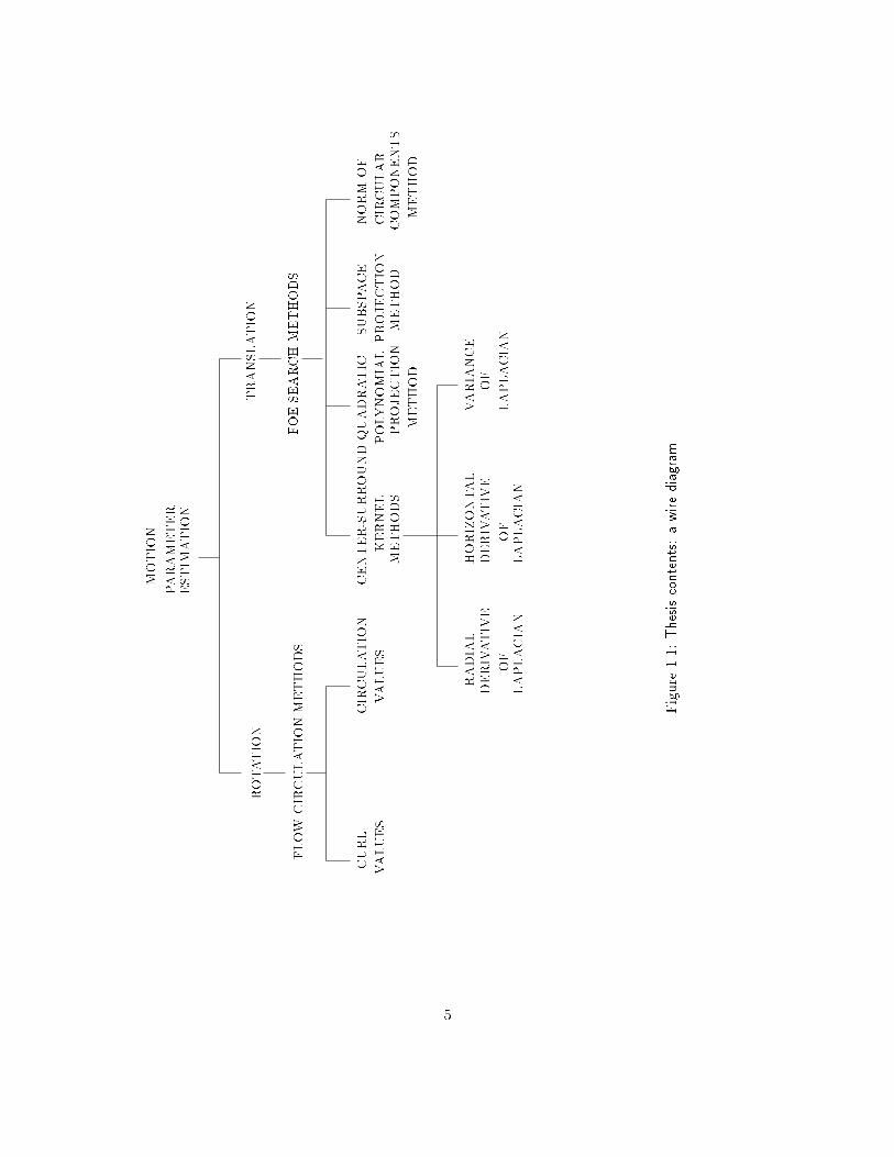
A wire diagram representing the contents of this thesis is shown in Fig. (1.1). The motion
parameter estimation is shown divided into two: rotational parameter estimation and translational
parameter estimation. The di�erent methods developed here appear at the leaves of the wire
diagram.
In Chapter 2, we present a review of existing methods for motion analysis. In Chapter 3,
we develop the relationship between the motion of a point in the three-dimensional scene and
the instantaneous vector that is observed on the image plane. In Chapter 4, we present the ow
circulation algorithm, a method to determine the rotational motion of the sensor. In Chapter 5,
we describe methods to estimate the translational motion of a sensor; these methods constitute the
FOE search algorithm. In Chapter 6, we analyze the applicability of the various methods presented
in the thesis, considering various scene and motion situations. In Chapter 7, experimental results
with synthetic data are presented. In Chapter 8, we present experimental results using real data,
4
METHOD
COMPONENTS
CIRCULAR
METHOD
PROJECTION
POLYNOMIAL
QUADRATIC
VALUES
VALUES
CIRCULATION
CURL
FLOW
CIRCULATIONMETHODS
ROTATION
ESTIMATION
PARAMETER
MOTION
CENTER-SURROUND
KERNEL
METHODS
SUBSPACE
PROJECTION
METHOD
NORM
OF
TRANSLATION
FOESEARCH
METHODS
RADIAL
DERIVATIVE
OF
LAPLACIAN
HORIZONTAL
DERIVATIVE
OF
LAPLACIAN
VARIANCE
OF
LAPLACIAN
Figure1.1:Thesiscontents:awirediagram.
5

and �nally provide a summary and directions for possible future work in Chapter 9.
6
Chapter 2
Review of Previous Work
2.1 Introduction
The problem of analyzing visual motion has attracted the attention of a lot of researchers.
It will be noted that a great majority of the work in visual motion analysis has been with the
extraction of structural information (structure from motion, or SFM). It is di�cult to do justice to
the numerous publications in this area. We will brie y survey the results that are relevant to the
material presented in this thesis. An extensive review of visual motion algorithms can be found
in [3]. A recent analysis of optical ow computation techniques is in Barron et. al. [7].
2.2 Problem statement
Our concern here is the situation where the sensor is in motion and the objects in the environment
are rigid and stationary; we would like to determine the motion of the camera. The other problem
of interest is to determine the structure of the environment. A more general scenario is one in
which not only the sensor is in motion, but some objects in the scene are also moving, as in the
case of driving on a busy highway; in addition, the objects in the scene could be non-rigid, like
clouds or people. It has been noted [72] that the imposition of the rigidity constraint is one way of
dealing with the ill-posedness of the problem. In our algorithms, we will restrict our attention to
the case of rigid, static objects.
Formally, the problem is, given a sequence of images, we would like to determine the motion
parameters (the translational and rotational velocities of the sensor). This is typically done in two
stages. In the �rst stage, a representation of the motion of image features is computed. This could
be in the form of a dense vector �eld denoting the instantaneous motion of intensity points. This
vector �eld is the optical ow �eld. Alternatively, one could compute the corresponding points in
two consecutive images. This is usually a sparse representation. In the second stage, the parameters
of motion and the structure of the scene are computed, using the representation produced by the
�rst stage. We begin by reviewing the methods for computing the optical ow; then we look at
7
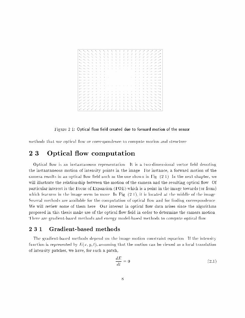
Figure 2.1: Optical ow �eld created due to forward motion of the sensor.
methods that use optical ow or correspondence to compute motion and structure.
2.3 Optical ow computation
Optical ow is an instantaneous representation. It is a two-dimensional vector �eld denoting
the instantaneous motion of intensity points in the image. For instance, a forward motion of the
camera results in an optical ow �eld such as the one shown in Fig. (2.1). In the next chapter, we
will illustrate the relationship between the motion of the camera and the resulting optical ow. Of
particular interest is the Focus of Expansion (FOE) which is a point in the image towards (or from)
which features in the image seem to move. In Fig. (2.1), it is located at the middle of the image.
Several methods are available for the computation of optical ow and for �nding correspondence.
We will review some of them here. Our interest in optical ow data arises since the algorithms
proposed in this thesis make use of the optical ow �eld in order to determine the camera motion.
There are gradient-based methods and energy model-based methods to compute optical ow.
2.3.1 Gradient-based methods
The gradient-based methods depend on the image motion constraint equation. If the intensity
function is represented by E(x; y; t), assuming that the motion can be viewed as a local translation
of intensity patches, we have, for such a patch,
dE
dt= 0 (2:1)
8
bright
dark
(Ex; Ey)
x
y
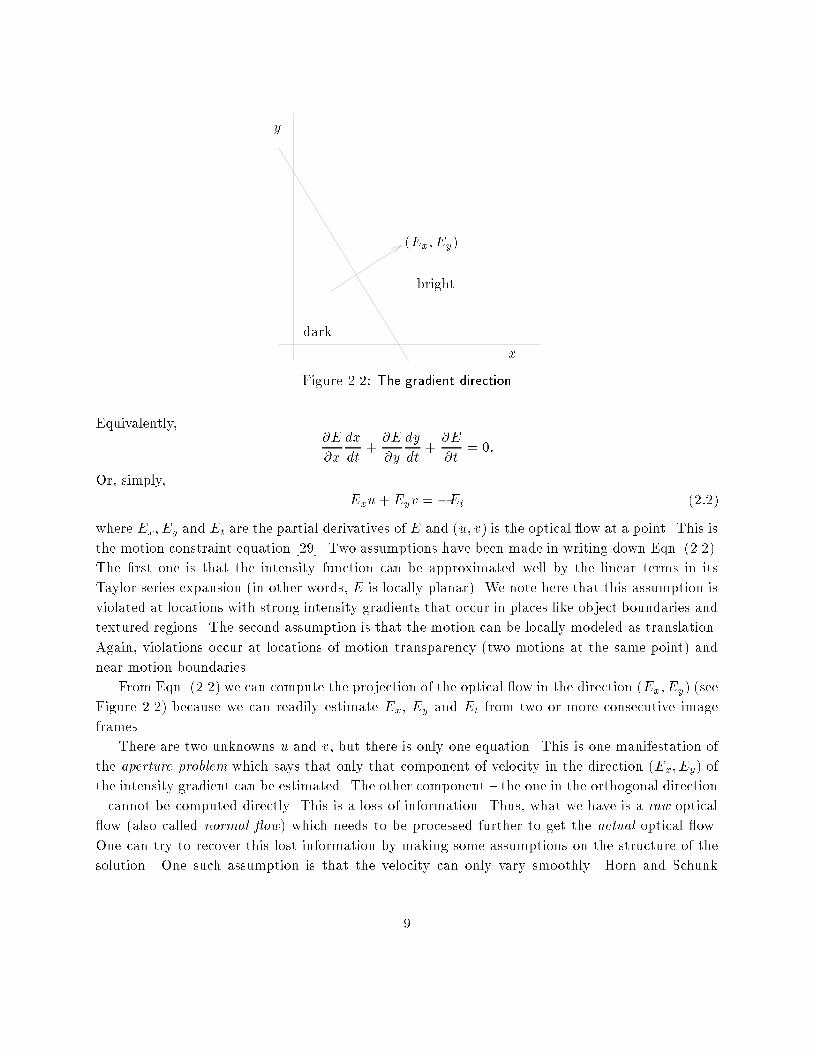
Figure 2.2: The gradient direction
Equivalently,@E
@x
dx
dt+@E
@y
dy
dt+@E
@t= 0:
Or, simply,
Exu+Eyv = �Et (2:2)
where Ex; Ey and Et are the partial derivatives of E and (u; v) is the optical ow at a point. This is
the motion constraint equation [29]. Two assumptions have been made in writing down Eqn. (2.2).
The �rst one is that the intensity function can be approximated well by the linear terms in its
Taylor series expansion (in other words, E is locally planar). We note here that this assumption is
violated at locations with strong intensity gradients that occur in places like object boundaries and
textured regions. The second assumption is that the motion can be locally modeled as translation.
Again, violations occur at locations of motion transparency (two motions at the same point) and
near motion boundaries.
From Eqn. (2.2) we can compute the projection of the optical ow in the direction (Ex; Ey) (see
Figure 2.2) because we can readily estimate Ex, Ey and Et from two or more consecutive image
frames.
There are two unknowns u and v, but there is only one equation. This is one manifestation of
the aperture problem which says that only that component of velocity in the direction (Ex; Ey) of
the intensity gradient can be estimated. The other component { the one in the orthogonal direction
{ cannot be computed directly. This is a loss of information. Thus, what we have is a raw optical
ow (also called normal ow) which needs to be processed further to get the actual optical ow.
One can try to recover this lost information by making some assumptions on the structure of the
solution. One such assumption is that the velocity can only vary smoothly. Horn and Schunk
9
v?
u?
V
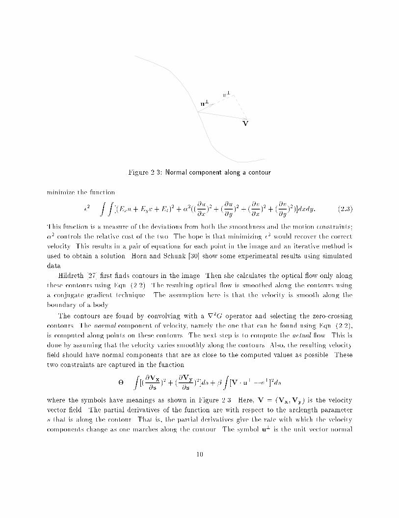
Figure 2.3: Normal component along a contour
minimize the function
�2 =Z Z
[(Exu+ Eyv +Et)2 + �2((
@u
@x)2 + (
@u
@y)2 + (
@v
@x)2 + (
@v
@y)2)]dxdy: (2:3)
This function is a measure of the deviations from both the smoothness and the motion constraints;
�2 controls the relative cost of the two. The hope is that minimizing �2 would recover the correct
velocity. This results in a pair of equations for each point in the image and an iterative method is
used to obtain a solution. Horn and Schunk [30] show some experimental results using simulated
data.
Hildreth [27] �rst �nds contours in the image. Then she calculates the optical ow only along
these contours using Eqn. (2.2). The resulting optical ow is smoothed along the contours using
a conjugate gradient technique. The assumption here is that the velocity is smooth along the
boundary of a body.
The contours are found by convolving with a r2G operator and selecting the zero-crossing
contours. The normal component of velocity, namely the one that can be found using Eqn. (2.2),
is computed along points on these contours. The next step is to compute the actual ow. This is
done by assuming that the velocity varies smoothly along the contours. Also, the resulting velocity
�eld should have normal components that are as close to the computed values as possible. These
two constraints are captured in the function
� =Z[(@Vx
@s)2 + (
@Vy
@s)2]ds+ �
Z[V � u? � v?]2ds
where the symbols have meanings as shown in Figure 2.3. Here, V = (Vx;Vy) is the velocity
vector �eld. The partial derivatives of the function are with respect to the arclength parameter
s that is along the contour. That is, the partial derivatives give the rate with which the velocity
components change as one marches along the contour. The symbol u? is the unit vector normal
10
y
x
(a)
x
y
t
(b)
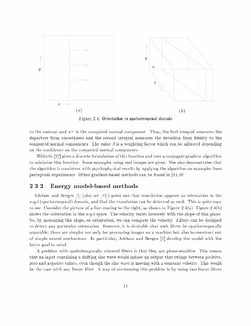
Figure 2.4: Orientation in spatiotemporal domain
to the contour and v? is the computed normal component. Thus, the �rst integral measures the
departure from smoothness and the second integral measures the deviation from �delity to the
computed normal components. The value � is a weighting factor which can be adjusted depending
on the con�dence on the computed normal components.
Hildreth [27] gives a discrete formulation of this function and uses a conjugate gradient algorithm
to minimize this function. Some examples using real images are given. She also demonstrates that
the algorithm is consistent with psychophysical results by applying the algorithm on examples from
perceptual experiments. Other gradient-based methods can be found in [44,49].
2.3.2 Energy model-based methods
Adelson and Bergen [1] (also see [12]) point out that translation appears as orientation in the
x-y-t (spatiotemporal) domain, and that the translation can be detected as such. This is quite easy
to see. Consider the picture of a line moving to the right, as shown in Figure 2.4(a). Figure 2.4(b)
shows the orientation in the x-y-t space. The velocity varies inversely with the slope of this plane.
So, by measuring this slope, or orientation, we can compute the velocity. Filters can be designed
to detect any particular orientation. However, it is desirable that such �lters be spatiotemporally
separable; these are simpler not only for processing images on a machine but also to construct out
of simple neural mechanisms. In particular, Adelson and Bergen [1] develop the model with the
latter goal in mind.
A problem with spatiotemporally oriented �lters is that they are phase-sensitive. This means
that an input containing a drifting sine wave would induce an output that swings between positive,
zero and negative values, even though the sine wave is moving with a constant velocity. This would
be the case with any linear �lter. A way of overcoming this problem is by using two linear �lters
11
whose responses are 90 degrees out of phase { called a quadrature pair { and by taking the sum of
squares of their outputs. An example of such a quadrature pair is a set of oriented Gabor �lters,
one with a cosine phase and the other with a sine phase.
The key observation behind another energy model is that the Fourier transform energy of a
translating image lies on a plane whose slope depends on the velocity of the movement. This can
be derived quite easily [60]. The idea behind Heeger's algorithm [22] is to estimate the orientation
of this plane by sampling the energy of the Fourier transform and by �tting a plane.
The sampling is done by Gabor �lters. A one-dimensional sine-phase Gabor �lter is given by
g(t) =1p2��
exp(�t
2
2�2) sin(2�!t)
The power spectrum is a pair of gaussians centered at ! and �!. Convolving this �lter with an
one-dimensional function is equivalent to multiplying their Fourier transforms. The result is a
sampling of the power spectrum of that function around ! and �!, yielding the Gabor energy.
Such a �lter is called a Gabor-energy �lter.
A sine-phase �lter and a cosine-phase �lter are convolved with the image sequence. The power
outputs are squared and added. This quadrature pair is employed to avoid the phase-dependency,
as outlined earlier in this section. The model uses a family of Gabor-energy �lters; the motion
energy is predicted by computing the response of the �lters to a random-dot texture translating
with velocity (u; v). This is an analytical expression involving u and v. The computed motion
energy has to be close to this predicted value if the pattern is moving with velocity (u; v). Thus, a
least-squares estimate for (u; v) can be found by minimizing some measure of the di�erence between
the computed and predicted motion energies. This amounts to �nding the plane that best �ts the
computed energy in the three dimensional Fourier space.
Other methods using spatiotemporal �ltering can be found in [62,15,18].
2.4 Correspondence computation
Many algorithms have been developed to solve the matching problem in stereo vision, where
there are two pictures of the same scene taken from two di�erent camera positions. This can be
considered equivalent to a camera motion; that is, the camera took the picture from one position
and then moved to the other position to take the second picture. However, this is only a particular
case of camera motion. In general, the camera could have a rotational movement; and it might
translate towards the objects. Also, objects in the scene might move. Thus, when compared to
stereo, the matching problem for motion applications is more di�cult. Matching can be done over
two frames at a time or over more frames. We describe a correlation based scheme [5] that computes
dense correspondence (i.e., for each pixel). We make use of an implementation of this scheme to
compute the optical ow �eld data for our motion computation.
Anandan's algorithm [5] matches features at multiple resolutions using a Laplacian pyramid
[11,10]. He �rst matches at the coarsest level where even a large-scale movement will be seen as
12
a sub-pixel displacement. The result is then passed onto �ner levels by an overlapped pyramid
projection scheme. The coarse estimate is used at the �ner level to get a better estimate of the
motion. The �nal estimates are obtained at the �nest level.
The Laplacian pyramid [10] can be constructed by �rst building a Gaussian low-pass-�lter
pyramid from the input image and then by computing the di�erence between adjacent levels of
the Gaussian pyramid. The result is a set of band-pass-�ltered images. The matching starts from
the coarsest level where the �ner details are not present. The matching is done using a correlation
scheme based on the minimization of the sum of squared di�erences (SSD) [59]. For every pixel
of the �rst image, a candidate pixel on the other image is found by using the results from the
coarser level. The SSD for this pair is a Gaussian weighted sum of the squared di�erences between
the values of the corresponding pixels in the 5 � 5 windows centered around the source and the
candidate pixels.
A pixel at level l in the pyramid passes its estimates to all the pixels in a 4� 4 area in the next
�ner level l+1. Thus each pixel receives estimates from 4 parents above (hence the name overlapped
pyramid projection scheme) , and the SSD measure is minimized over these. A con�dence measure
is established by observing the following: the location of the minimum of the SSD which is supposed
to give the disparity is frequently not at the exact disparity. Its distance from the actual disparity
depends on the type of surface being matched: the best is for unoccluded corner points and the
worst for homogeneous surfaces and occluded corner points. The accuracy of the match can be
estimated by �nding the local curvature of the SSD surface. The larger the curvature, the more
accurate the answer is. This con�dence measure, which is useful in the smoothing process, consists
of two magnitudes (cmax and cmin) and two direction vectors (emax and emin, which are the unit
vectors along the principal axes of the SSD surface). The magnitudes are given by
cmax =Cmax
k1 + k2Smin + k3Cmax
and
cmin =Cmin
k1 + k2Smin + k3Cmin
where k1, k2 and k3 are normalization parameters, Smin is the SSD value corresponding to the best
match, and Cmax and Cmin are the curvatures of the SSD surface along the axes of maximum and
minimum curvature.
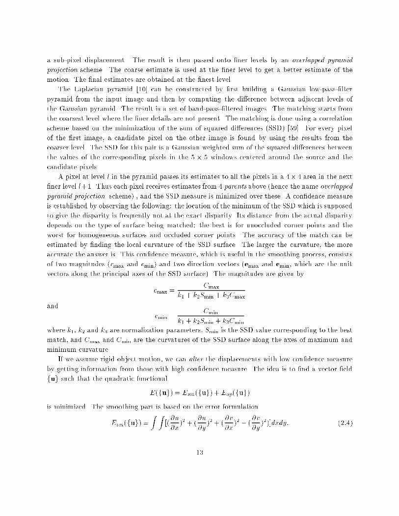
If we assume rigid object motion, we can alter the displacements with low con�dence measure
by getting information from those with high con�dence measure. The idea is to �nd a vector �eld
fug such that the quadratic functional
E(fug) = Esm(fug) + Eap(fug)is minimized. The smoothing part is based on the error formulation
Esm(fug) =Z Z
[(@u
@x)2 + (
@u
@y)2 + (
@v
@x)2 + (
@v
@y)2)]dxdy: (2:4)
13
where fug is the set of the displacement vectors u(x; y) = (u(x; y); v(x; y)). The function in
Eqn. (2.4) is the same as in Eqn. (2.3), except that Esm(fug) contains only the smoothness con-
straint. The approximation error Eap measures how well the computed �eld approximates the
measured displacement �eld:
Eap(fug) =Xx;y
[cmax(u � emax� d � emax)2 + cmin(u � emin � d � emin)
2]
where d gives the match estimate at each point. Minimizing the error function E(fug) in discrete
form results in a system of coupled linear equations and is solved using the Gauss-Seidel relaxation
algorithm. After the displacements and the associated con�dences are computed within each level,
the displacement �eld is smoothed before it is projected to the next level in the pyramid.
This algorithm gives good qualitative results in most regions of images [5], but has problems with
occluded regions and at motion boundaries. For instance, displacements in areas of background
near the boundary of a moving object are in uenced by the moving object; occluded areas do
not have reliable local estimates, and so the more reliable estimates from the neighborhood are
propagated into these areas.
Barnard and Thompson [6] give an iterative relaxation algorithm which tries to �nd the best
possible match for two sets of points (features) in two images. First, a set of candidate points are
chosen from each image by using some interest point detection technique, such as the Moravec's
operator [48]. The next step is to determine the matching. For each point Pi in the �rst image,
a set of candidate points are chosen from the second image as those within some distance from Pi
(compute this distance by imagining that Pi is in the second image). With each Pi, we associate a
set Li of labels. Each label l is either a disparity vector or a distinguished symbol l�. Each label
is a potential disparity for that point; l� means that no match in the second image and hence no
disparity can be assigned to the point. Initially Li contains only a l�. In addition, there is a number
pi(l) associated with each label l which can be interpreted as the probability that the point Pi has
disparity l. A relaxation procedure iteratively modi�es all these probabilities so that for each point
one of the probabilities, say, that of label l1 is expected to dominate while the others tend to zero.
This suggests that l1 is the disparity for that point.
The algorithm proposed by Sethi and Jain [61] uses more than two images in a time sequence to
�nd matching points. The main idea is path coherence which says that the trajectory traced by a
point is smooth. The trajectory of a point is the curve connecting it through all its matching points
in the sequence. The fundamental assumption here is that objects are in constant motion, without
undergoing sudden changes in their movements. A measure of the smoothness of the trajectory is
de�ned and it is minimized to get the best match satisfying path coherence.
An algorithm that combines both a gradient-based method and a feature-based method has
been proposed by Heitz and Bouthemy [25]. It is based on a Bayesian formulation using Markov
random �elds. The motion constraint in Eqn. (2.2) is used to compute ow, simultaneously with a
Moving Edge constraint described in [8]. Validation factors are de�ned for each of these constraints.
14
C1C2
m2m1
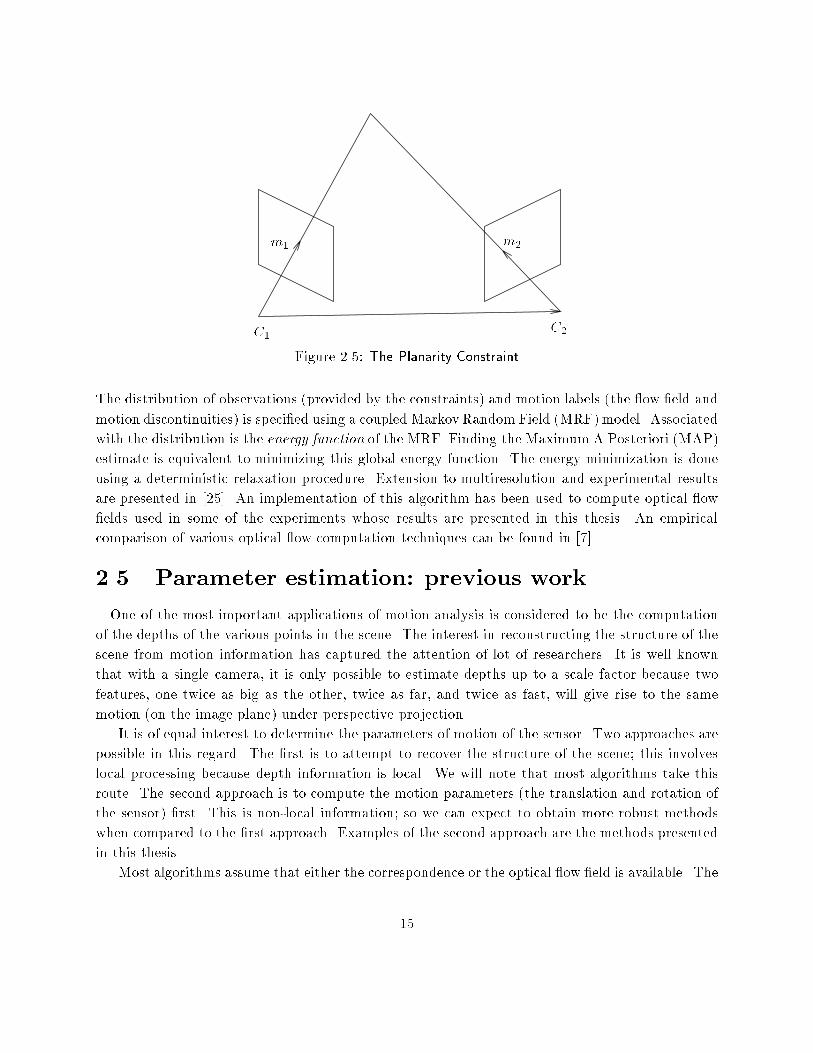
Figure 2.5: The Planarity Constraint
The distribution of observations (provided by the constraints) and motion labels (the ow �eld and
motion discontinuities) is speci�ed using a coupled MarkovRandom Field (MRF)model. Associated
with the distribution is the energy function of the MRF. Finding the Maximum A Posteriori (MAP)
estimate is equivalent to minimizing this global energy function. The energy minimization is done
using a deterministic relaxation procedure. Extension to multiresolution and experimental results
are presented in [25]. An implementation of this algorithm has been used to compute optical ow
�elds used in some of the experiments whose results are presented in this thesis. An empirical
comparison of various optical ow computation techniques can be found in [7].
2.5 Parameter estimation: previous work
One of the most important applications of motion analysis is considered to be the computation
of the depths of the various points in the scene. The interest in reconstructing the structure of the
scene from motion information has captured the attention of lot of researchers. It is well known
that with a single camera, it is only possible to estimate depths up to a scale factor because two
features, one twice as big as the other, twice as far, and twice as fast, will give rise to the same
motion (on the image plane) under perspective projection.
It is of equal interest to determine the parameters of motion of the sensor. Two approaches are
possible in this regard. The �rst is to attempt to recover the structure of the scene; this involves
local processing because depth information is local. We will note that most algorithms take this
route. The second approach is to compute the motion parameters (the translation and rotation of
the sensor) �rst. This is non-local information; so we can expect to obtain more robust methods
when compared to the �rst approach. Examples of the second approach are the methods presented
in this thesis.
Most algorithms assume that either the correspondence or the optical ow �eld is available. The
15
algorithm of Longuet-Higgins [41] (see also [71],[13] and [80] ) assumes that the correspondence of
points between two consecutive frames is available. The quantities computed are the translation ~t
and the rotation R for moving the camera from C1 to C2 (see Fig. (2.5)). The constraint for every
matching pair (for instance, m1 and m2 in Fig. (2.5)) is that the lines of projection for these two
image points meet in space (simply because they are the images of the same world point). This
planarity constraint can be expressed as follows:
~C1m1 � ~t �R ~C2m2 = 0 (2:5)
Equivalently,~C1m1 � TxR ~C2m2 = 0
where Tx is a matrix formed out of the elements of ~t. The constraint, applied to each pair of
corresponding points, results in an equation linear in the elements of the matrix E = TxR. With
correspondence for eight points, we obtain eight equations as in Eqn. (2.5) and we can solve for the
elements of the matrix E. From E, we can compute the translation vector ~t and the rotation matrix
R, as described in [41] or in [13]. The algorithm in [13] is more robust because it uses redundancy
to combat noise. That is, it uses more than eight points in solving for E. A cogent presentation of
the method can be found in [80].
Another algorithm, based on optical ow �eld input, is described by Heeger and Jepson [24].
This makes use of the bilinear form of the optical ow equations:
~�(x; y) = A(x; y; T )p(x; y)+ B(x; y)~! (2:6)
where ~�(x; y) is the optical ow at (x; y), T is the three parameters of the translation of the camera
and ~! is the vector of rotations with respect to the three axes. The 2� 3 matrix B depends only
on the image position (x; y) and the 2 � 1 matrix A depends only on the image position and the
translation T . The inverse depth is denoted by p(x; y). By choosing the optical ow at �ve points,
the Eqn. (2.6) can be rewritten in the form
~� = C(T )~r
where ~� is a 10� 1 vector of optical ow at the �ve points, C(T ) is a 10� 8 matrix depending on
the translation T and ~r is a 8 element vector consisting of the inverse depths of the �ve points and
the three axis rotations. Since ~� has to be in the range of the matrix C(T ), the appropriate value
of T can be determined by minimizing the projection of ~� on the space which is the orthogonal
complement to the range of C(T ). Knowing T , the rotations can also be computed [23]. We will
return to this algorithm again to point out the similarity it bears to some methods described in
this thesis.
Analysis of the optical ow �eld, also called the motion parallax �eld, has received considerable
research attention. J. J. Gibson, in 1950, discussed the motion parallax �eld, and de�ned and
16
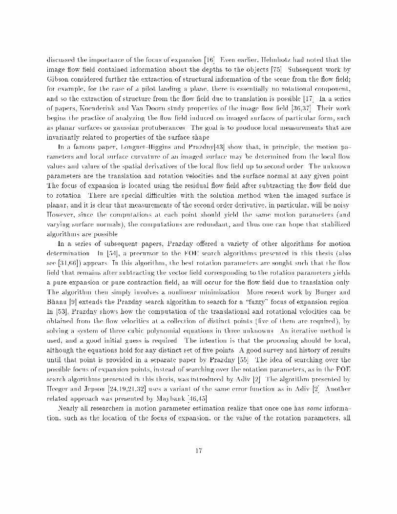
discussed the importance of the focus of expansion [16]. Even earlier, Helmhotz had noted that the
image ow �eld contained information about the depths to the objects [75]. Subsequent work by
Gibson considered further the extraction of structural information of the scene from the ow �eld;
for example, for the case of a pilot landing a plane, there is essentially no rotational component,
and so the extraction of structure from the ow �eld due to translation is possible [17]. In a series
of papers, Koenderink and Van Doorn study properties of the image ow �eld [36,37]. Their work
begins the practice of analyzing the ow �eld induced on imaged surfaces of particular form, such
as planar surfaces or gaussian protuberances. The goal is to produce local measurements that are
invariantly related to properties of the surface shape.
In a famous paper, Longuet-Higgins and Prazdny[43] show that, in principle, the motion pa-
rameters and local surface curvature of an imaged surface may be determined from the local ow
values and values of the spatial derivatives of the local ow �eld up to second order. The unknown
parameters are the translation and rotation velocities and the surface normal at any given point.
The focus of expansion is located using the residual ow �eld after subtracting the ow �eld due
to rotation. There are special di�culties with the solution method when the imaged surface is
planar, and it is clear that measurements of the second order derivative, in particular, will be noisy.
However, since the computations at each point should yield the same motion parameters (and
varying surface normals), the computations are redundant, and thus one can hope that stabilized
algorithms are possible.
In a series of subsequent papers, Prazdny o�ered a variety of other algorithms for motion
determination. In [54], a precursor to the FOE search algorithms presented in this thesis (also
see [31,66]) appears. In this algorithm, the best rotation parameters are sought such that the ow
�eld that remains after subtracting the vector �eld corresponding to the rotation parameters yields
a pure expansion or pure contraction �eld, as will occur for the ow �eld due to translation only.
The algorithm then simply involves a nonlinear minimization. More recent work by Burger and
Bhanu [9] extends the Prazdny search algorithm to search for a \fuzzy" focus of expansion region.
In [53], Prazdny shows how the computation of the translational and rotational velocities can be
obtained from the ow velocities at a collection of distinct points (�ve of them are required), by
solving a system of three cubic polynomial equations in three unknowns. An iterative method is
used, and a good initial guess is required. The intention is that the processing should be local,
although the equations hold for any distinct set of �ve points. A good survey and history of results
until that point is provided in a separate paper by Prazdny [55]. The idea of searching over the
possible focus of expansion points, instead of searching over the rotation parameters, as in the FOE
search algorithms presented in this thesis, was introduced by Adiv [2]. The algorithm presented by
Heeger and Jepson [24,19,21,32] uses a variant of the same error function as in Adiv [2]. Another
related approach was presented by Maybank [46,45].
Nearly all researchers in motion parameter estimation realize that once one has some informa-
tion, such as the location of the focus of expansion, or the value of the rotation parameters, all
17
other parameters are easily obtained. Hence there is considerable motivation for separating the
ow �eld due to rotational parameters from the ow �eld due to translational parameters. Already
noted by Helmholtz [75] and mentioned by Longuet-Higgins and Prazdny[43] is the idea of making
use of either depth discontinuities or motion parallax of a translucent surface (such as a dusty
window). In these cases, the di�erence or jump in the ow velocities cancels the ow component
due to the rotational parameters, leaving a ow dependent only on translational parameters. Pro-
viding there are enough such points, then the focus of expansion, and hence all other parameters,
may be determined. Lawton and Rieger exploit this idea to build a system based on di�erences of
neighboring ow velocities [57]. Unfortunately, noise tends to make this method rather unreliable.
Lawton built another system that assumes that the rotational parameters are nearly zero, and thus
�nds the focus of expansion by means of a \Hough transform" technique [39]. A solution method
that assumes that the translational parameters are zero would be quite easy; the ow circulation
method presented in this thesis (also in [68]) provides an exact procedure, and other methods are
straightforward.
In a series of papers, Waxman and collaborators revisited the problem of motion parameter
estimation and local surface structure determination from local ow parameters (i.e., values of the
ow velocities and derivatives of the ow velocities through second order). A solution method is
presented for the case of planar surface patches and quadratic ow velocity �elds [65] together
with an analysis of the ambiguities, followed by a new method for quadratic surfaces and quadratic
velocity �elds [77] which improves upon an earlier method of Waxman and Ullman [78]. More detail
and extensions to binocular image ows are given in [82]. In all of these works, the structure of the
surface and the motion parameters are considered as the unknowns relative to a single image point.
That is, the analysis is local. Measurements must be given of derivatives of ow velocity values
through second order, in which case it is possible to solve for local surface structure up to a second
order Taylor expansion. The curl of the ow �eld is one of the twelve \deformation parameters"
(D6 to be exact), and the \kinematic relation" for this parameter is precisely the equation that we
require for the ow circulation algorithm. However, since the problem that Waxman addresses is
the exact computation of motion parameters coupled with surface parameters based upon local data
(deformation data at a single point), the approximations and the global method leading to the ow
circulation algorithm is missed. Using instead correspondences of curves, the local quadratic nature
of the velocity �eld can be obtained providing a su�cient number of curves are matched, as studied
by Wohn [79,82] (who also makes use of some temporal smoothing). Solution methods based on
the use of a su�cient number of correspondences of points, without involving explicit derivatives
of the ow �eld, and without explicit representation of surface parameters, are provided by Jerian
and Jain [33]; their work, like that of Tsai and Huang [71] is directed for the case of determining
rotation and translation parameters from correspondences, as opposed to rotation and translation
velocities from an image velocity ow �eld. An approach to factor a matrix of motion measurements
into two matrices that represent shape and motion, for the case of orthographic projection has been
18
proposed by Tomasi and Kanade [70]. Direct methods for recovering the motion parameters have
been described by Horn and coworkers [28,52]. The direct methods apply only for restricted kinds
of motion, such as pure translation.
Clearly, the surface parameters, to the extent that they can be recovered, must be based on
local measurements. The motion parameters, however, are global. Most researchers have noted
that their methods provide redundant computation of motion parameters, providing a test for
the rigidity assumption. Unfortunately, many of the algorithms forgo the stability that can be
obtained by deriving the motion parameters from an integrative approach i.e., by making use of
the constancy over the image. Of course, if one's focus is on surface parameter reconstruction, then
local processing is essential. However, if one �rst derives the motion parameters, and then uses
knowledge of the motion parameters to assist in surface depth estimates, then global methods may
be used for motion parameter estimation. Methods that can potentially make use of distributed
information include those of Prazdny [53], Adiv [2], and Heeger and Jepson [21].
The curl of the ow �eld, which is the basis of our ow circulation algorithm, has long been
recognized as an important property of the motion �eld. However, the observation that the curl
of the �eld is approximated by a linear function, and the use of that approximation to determine
the rotational parameters, appears to be new. Koenderink and Van Doorn [36] calculate explicitly
the curl (and other functionals). We begin with their computation of the curl (converted to planar
image coordinates as opposed to polar coordinates), but make use of the function to solve for the
rotational parameters. They instead studied the properties of these elementary �elds in the case of
an observer moving with respect to a plane [37,38]. The existence of receptive �elds sensitive to the
curl (and also to the divergence) was hypothesised by Koenderink and Van Doorn [36] and Longuet-
Higgins and Prazdny [43], but the motivation is for surface structure determination, and not for
global synthesis of motion parameters. Regan and Beverly [56] followed up on the hypothesis of
Longuet-Higgins and Prazdny by conducting psychophysical experiments, and concluded that the
existence of vorticity receptors is plausible. Cell recordings in the dorsal part of MST of Macaque
monkeys suggest cells tuned to expansion/contraction and other cells sensitive to rotation [69].
More recently, Werkhoven and Koenderink [81] have considered methods for directly computing
ow �eld invariants, including the curl, from time-varying image irradiance data. The considerable
interest and evidence for the importance of the curl of the ow �eld, or equivalently, the circulation
values, lends credence to the ow circulation algorithm presented in this thesis.
In the next chapter we relate the optical ow �eld to the motion parameters of the sensor. The
model so obtained would enable us to point out how one can estimate the motion parameters by
suitably processing the optical ow �eld.
19
Chapter 3
The Optical Flow Equations
3.1 Introduction
We consider the imagery that is produced by a moving sensor. The sensor produces images whose
contents are altered over time due to either the motion of the sensor, or the motion of objects in
the scene, or both. Thus, two kinds of motion are possible: sensor motion and object motion. The
sensor could move about in its environment. A camera mounted on an Autonomous Land Vehicle
is one example. On the other hand, objects in the scene could move. In general, both kinds of
motion can happen simultaneously. Mathematically, it is natural to consider the relative motion
between the sensor and each of the objects in the scene. The prerequisite for using relative motion
in image processing is the availability of segmented images, namely, the segregation of the di�erent
objects in each image. This would conceivably be done at an earlier stage of processing, using
either a static segmentation technique operating on each image in turn or a dynamic method using
the motion information obtained from more than one image.
Optical sensors like the retina or a camera �lm are sensitive to illumination; so, the motion
information is available as changes in the illumination intensity patterns falling on the sensor array.
The instantaneous movement of the intensity pattern on the sensor array can be represented by
a vector �eld; the vector �eld value at location P represents the instantaneous motion of the
pattern at the point P . The vector �eld is referred to as the optical ow �eld, or simply, the ow
�eld. It is customary to assume that the ow �eld represents a projection of the instantaneous
three-dimensional motion even though this is not always true [74].
We need to model the ow �eld in terms of the parameters of the real world motion and the
structure of the environment, in order to interpret the ow �eld. The aim of this chapter is to
present a model of the ow �eld as a set of equations that relate the ow �eld to the motion
parameters and the scene structure, and to make certain observations about the form of these
equations.
One of the issues in the modeling is the choice of a coordinate system. The coordinate system
can be either ego-centric or exo-centric. The ego-centric system is one in which the coordinate
20
system is �xed with respect to the sensor (typically, the origin will be located within the sensor).
This means that the coordinates of a point that is not rigidly attached to the sensor will change
with time as the sensor moves. In the exo-centric system, the coordinate system is located outside
the sensor, usually in a static location or object.
A second, less critical choice concerns the representation which is typically either cartesian or
spherical. The cartesian coordinate system is a natural choice for cameras with a planar imaging
array, and the spherical coordinate system is the best choice for the human eye because the retina
is roughly spherical.
In this chapter, we derive the optical ow equations for an ego-centric cartesian coordinate
system and observe some of the properties of these equations. The results could be derived in other
coordinate systems, but would be more complicated.
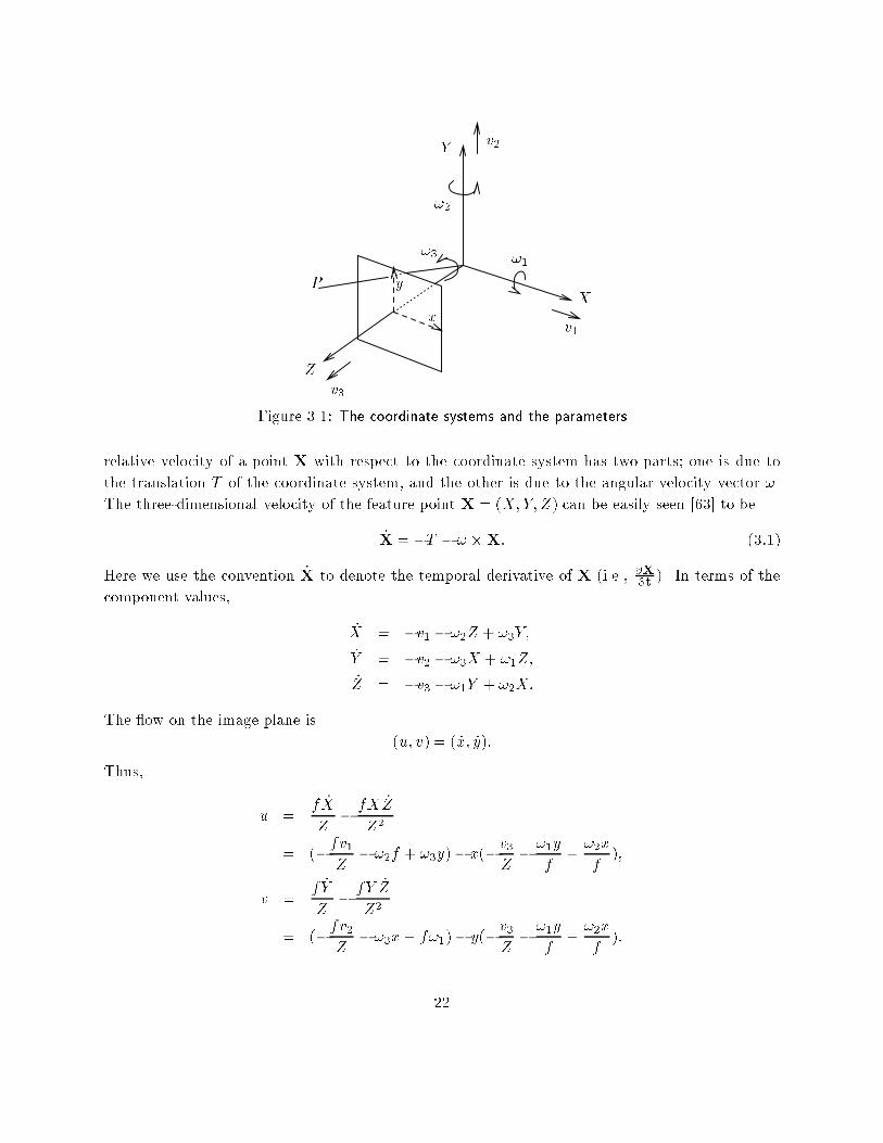
3.2 The coordinate systems
The optical ow equations for the perspective projection of a scene on a planar imaging sensor are
well-known and understood. We provide here an independent derivation, similar to the development
in [21,29,43]. We will adopt the cartesian coordinate system and the motion parameters as shown in
Fig. (3.1). The three-dimensional coordinate system is centered at the camera's center of projection
and the coordinates are denoted using upper-case letters X , Y and Z. This is the sensor coordinate
system. The imaging surface is a plane located at Z = f , f being the focal length. The x and y
coordinate axes lie on this plane, with the origin at the center of the image. The transformation
from spatial coordinates to the image coordinates is given by the equations of perspective projection
which can be easily derived using a pin-hole approximation to the lens:
x = fX=Z; y = fY=Z
where (X; Y; Z) = (X(x; y); Y (x; y); Z(x; y)) is the position of the point in three-dimensional space
that is imaged at (x; y). We assume that the objects in the scene are �xed and rigid. We want
to determine the ow �eld which is observed due to the motion of the sensor, as a function of the
image coordinates x and y.
The camera moves with a translational velocity of T = (v1; v2; v3) and a rotational velocity of
! = (!1; !2; !3). The values v1, v2 and v3 are the X , Y and Z components of the instantaneous
vector describing the translation of the sensor. The rotation that the sensor coordinate system
undergoes can be described either using a rotation matrix R, or equivalently, by the angular velocity
magnitude M! about an axis of rotation A!. In the latter case, one can simplify the details by
de�ning an angular velocity vector ! that has magnitude M! and direction A!. Again, !1, !2 and
!3 are the components of !.
The optical ow V = (u; v) at the image point (x; y) can be obtained by projecting the three-
dimensional relative velocity of the feature point X imaged at (x; y) onto the image plane. The
21
X
v3
v2
v1
P y
x
!3
!2
!1
Y
Z
Figure 3.1: The coordinate systems and the parameters
relative velocity of a point X with respect to the coordinate system has two parts; one is due to
the translation T of the coordinate system, and the other is due to the angular velocity vector !.
The three-dimensional velocity of the feature point X = (X; Y; Z) can be easily seen [63] to be
_X = �T � ! �X: (3:1)
Here we use the convention _X to denote the temporal derivative of X (i.e., @X@t
). In terms of the
component values,
_X = �v1 � !2Z + !3Y;
_Y = �v2 � !3X + !1Z;
_Z = �v3 � !1Y + !2X:
The ow on the image plane is
(u; v) = ( _x; _y):
Thus,
u =f _X
Z�fX _Z
Z2
= (�fv1Z� !2f + !3y)� x(�
v3Z�!1y
f+!2x
f);
v =f _Y
Z�fY _Z
Z2
= (�fv2Z� !3x+ f!1)� y(�
v3Z�!1y
f+!2x
f):
22
Making explicit the dependence on the image coordinates and rearranging terms, we get
u(x; y) = 1Z(x;y) [�fv1 + xv3] + !1
hxyf
i� !2
hf + x2
f
i+ !3y;
v(x; y) = 1Z(x;y) [�fv2 + yv3] + !1
hf + y2
f
i� !2
hxyf
i� !3x:
(3:2)
Here, u(x; y) and v(x; y) are the x and y components of the optical ow �eld V (x; y).
In a similar fashion, one can derive the equations of the ow �eld for a spherical imaging surface.
All procedures that work in the cartesian coordinate system can be transformed to work in the
spherical coordinate system.
3.3 Observations on the equations
The equations in (3.2) have certain properties that we note here. The ow equations may be
grouped into the sum of two terms, as is noted, for example, in [43]: the �rst term gives the ow
�eld due to the translational components, and is modulated by the inverse depths, and the second
term is a ow �eld due to the rotational components, and is independent of the depths. Thus,
V (x; y) =
"u(x; y)
v(x; y)
#= Vv(x; y) + V!(x; y); (3:3)
with (for the case v3 6= 0)
Vv(x; y) = v3�(x; y)
"x � �
y � �
#;
� =fv1v3
; � =fv2v3
; �(x; y) =1
Z(x; y)(3.4)
and
V!(x; y) = !1
"xyf
f + y2
f
#+ !2
"�f � x2
f�xyf
#+ !3
"y
�x
#: (3:5)
The ow due to the translational components has a radial structure, expanding or contracting
about a focus of expansion at location (�; �) and with a magnitude modulated by the distance from
the focus of expansion, the component of translation in the viewing direction (v3), and the inverse
depth to the point imaged at each pixel, �(x; y) = 1=Z(x; y). In the case v3 = 0, the situation is
nearly the same, except that Vv is now a parallel vector �eld:
Vv(x; y) = �f�(x; y)
"v1v2
#(v3 = 0); (3:6)
in the direction of the translational velocity, modulated by inverse depths as before. In both cases,
the ow due to the rotational components is the linear combination of three �xed ow �elds,
weighted by the angular (rotational) velocity components.
23
The rotational part, namely V!, is linear (see Eqn. (3.5)) in the rotational parameters ! =
(!1; !2; !3). On the other hand, the translational part Vv(x; y) is bilinear, i.e., linear in �(x; y) for
�xed translation T and linear in T for �xed inverse depths �(x; y). In essence, the translational
parameters appear in product form with the inverse depth values (note the forms v1Z, v2
Zand v3
Z
appearing in Eqn. (3.2)). We can multiply both the translation vector T and the depth function
Z(x; y) by the same factor, say a constant k, and the equations (3.2) will still hold. Thus, it is
not possible to recover the absolute values of the translational parameters and the absolute inverse
depths. They can be estimated only up to a scale factor; only relative depths can be computed from
a monocular image sequence, and only two translational parameters can be recovered. There is a
need to choose a unit of measure. A good choice for the unit of distance measure is the translation
vector; the depth value corresponding to a feature point in units of the translation vector indicates
how long it will take for the camera to hit that feature point if moving towards it. For such a choice,
the translation vector is necessarily of unit length (i.e., with its tip on a unit sphere). Heeger and
Jepson [20] make use of this normalization and search for the translation vector by tessellating the
surface of a unit sphere.
Another possible normalization is to set one of the motion parameters to be unity. For instance,
if we choose v3 to be unity (for v3 6= 0), the other two are measured in terms of v3. The focus of
expansion (FOE) is precisely this. Recall from Eqn. 3.4 that the FOE is de�ned by (� = fv1v3; � =
fv2v3
), for the case v3 6= 0, and (� = fv1; � = fv2), for v3 = 0. We will adopt this choice and in a
later chapter present methods to compute the FOE.
If the structure of the scene (and hence �(x; y)) is known, the optical ow equations are linear
in all the motion parameters and can be easily solved, given a su�cient number of ow vectors.
However, it is seldom the case that �(x; y) is known except in certain controlled situations. Alter-
natively, if the translation T is known, then one can solve for the rotational parameters ! and the
scene structure because the equations will now be linear in the unknowns. In a general situation
where none of these quantities is known, it is possible to consider a collection of ow vectors re-
sulting in a system of nonlinear equations and solve for the unknowns. Note that we obtain two
equations per ow vector. The unknowns are the �ve motion parameters and one inverse depth per
ow vector position. Thus, given the ow vectors at �ve or more points, it is possible to solve for all
the unknowns. However, solving the set of nonlinear equations is non-trivial and the performance
of procedures to do this rely on a good initial guess. Some methods along these lines are presented
by Horn [29].
The �nal comment here concerns the appropriateness of using measured optical ow in con-
junction with the model in Eqns. (3.2). The optical ow that is induced on the imaging surface
is treated as a vector �eld that is a projection of the three-dimensional velocity of the feature in
motion. The optical ow does not necessarily always correspond to such a projection. One example
where such a correspondence does not hold is that of a rotating, featureless sphere. Optically, no
motion is seen even though there is physical movement. A formal treatment of the distinction
24
between the projection and the optical ow was done by Verri and Poggio [74]. They use the term
\motion �eld" to denote the projection of the three-dimensional velocity vectors, and point out that
the motion �eld and the optical ow are same only under certain conditions such as high contrast.
However, note that only the optical ow can be computed from the intensity images whereas the
motion �eld is the one that is easier to model. Also, modeling the optical ow requires assumptions
about illumination and surface re ectance properties; it is hard to choose the right assumptions.
Therefore, it is customary to assume that the motion �eld and the optical ow are the same, as we
do here.
In the approaches presented in this thesis, we will attempt to cancel out the contribution from
either the translation or the rotation, thus enabling us to estimate the other. The ow circulation
algorithm presented in the next chapter eliminates the translational part of the ow �eld in order
to estimate the rotational parameters. The FOE search algorithms presented in a later chapter
cancel the rotational part to estimate the focus of expansion. The focus of expansion is directly
related to the translational parameters.
25
Chapter 4
Rotational parameter estimation
4.1 Introduction
An object in motion can have both translational and rotational motion. For many applications,
it is necessary to determine the translational and rotational velocity. For instance, the sensor
on a spinning satellite may need to determine the angular velocity to adjust the motion of the
satellite. The source of a sensor's rotational velocity may be due to an intentional movement,
or due to vibrations. A helicopter in a turning ight has a rotational velocity that is nonzero.
A camera mounted on a vehicle that is moving on a rough terrain could experience vibrations
that produce an e�ect as though the camera is rotating about an axis that is changing rapidly.
In either case, it is important to determine the instantaneous rotational parameters. In the case
of the helicopter, the rotational parameters provide valuable information about the motion itself
while in the latter case, the estimated rotational parameters will be useful to eliminate the \jitter"
produced by the vibrations. In general, it is well known that estimation of the rotational parameters
helps to eliminate the rotational component of the ow �eld; this leaves behind the translational
component from which the translational parameters and the depth map can be computed by simple
algorithms. While this observation is theoretically sound, errors introduced in the estimation of
one set of parameters compound the errors that appear in the second stage of processing, namely
in estimating the other set of parameters.
Presented in this thesis are two independent algorithms, one to estimate the rotational param-
eters and the other to estimate the translational parameters, providing independent pathways to
estimate the di�erent parameters, thus eliminating the compounding of errors. We begin by �rst
presenting an algorithm to determine the rotational parameters.
We should note here that the rotational parameters depend on the choice of the origin. If the
location of the motive power for the physical rotation is known, one can choose that location to be
the origin of the model. In such a case, pure rotation (i.e., no translation) will be estimated as pure
rotation with respect to an axis passing through the chosen origin. However, if the mechanism for
the source of rotation is unknown, the natural choice for the origin is the focal point of the sensor.
26
In such a case, if the rotation axis does not pass through the origin, the rotation will be seen as a
combination of a rotation with respect to an axis through the chosen origin and a translation. Note
that once the quantities are estimated with respect to one choice of the origin, they can always be
transformed for another choice; the judgement of egomotion is thus una�ected by the choice.
The angular velocity ! of the sensor induces an image ow �eld that depends only on the
physical location of the image points and not on their depths. It is the ow �eld due to the
translation that depends on the depth to scene points. Looking at the equations of optical ow,
u(x; y) = 1Z(x;y) [�fv1 + xv3] + !1
hxyf
i� !2
hf + x2
f
i+ !3y;
v(x; y) = 1Z(x;y) [�fv2 + yv3] + !1
hf + y2
f
i� !2
hxyf
i� !3x;
(4:1)
we again note that the optical ow �eld is a vector sum of two ow �elds, one arising due to the
translation and the other arising due to the rotation:
V (x; y) = V v(x; y) + V !(x; y):
Also, note the linearity of the ow �eld in !. The method described here attempts to cancel the
contribution from translation and the depth values, while still retaining the linearity in !. We
show here that under certain assumptions, this is exactly possible, and under other conditions, it
is achieved in a global approximate sense. We provide the background mathematics, the technical
derivation and a description of the algorithm which will be called the ow circulation algorithm.
An analysis of the e�ect of violations of the assumptions is contained in Chapter 6. Experimental
results are presented in Chapters 7 and 8.
4.2 Curl and circulation values
The main observation behind the algorithm is that the curl of the ow vector �eld produces two
terms: A term that is linear in the rotational parameters, and a term that is dependent on the
translational parameters as well as the depth gradient. Under suitable conditions, we argue that
the latter contribution can be ignored, yielding an approximate linear method to determine the
rotational parameters.
We begin by reviewing the curl of a vector function and a related theorem which will be useful
to us. The curl of a two-dimensional vector �eld V (with u and v as the x and y components),
also denoted by r�V, is de�ned as
r�V =@v
@x�
@u
@y:
To be precise, this is the pointwise magnitude of a vector �eld in a direction orthogonal to the
two-dimensional plane containing the vector �eld V. Since the whole (curl) �eld is pointed in the
same direction, we will use the curl as though it is a scalar function. If the vector �eld V lies on a
27
spherical retina instead of a planar surface, then the curl values will point in a direction orthogonal
to the spherical surface. Here we are concerned only with the planar imaging surface.
An important property of the curl of a vector �eld is provided by Stoke's theorem [26]:
Z ZD
r�V dx dy =I@D
V � ds; (4:2)
where the right hand side, which we will call the circulation of the ow about the circuit @D,
denotes the contour integral of the vector �eld about the boundary of D. The theorem is quite
general, requiring only certain di�erentiability conditions on V and the boundary of the domain D.
Note that the contour integral is independent of the parameterization of the contour. For example,
when D is a disk of radius r about an image point (x0; y0), the circulation may be calculated from
I@D
V � ds =
Z 2�
0V (x0 + r cos �; y0 + r sin �) � (�r sin �; r cos �)d�:
Mitiche, Grisell and Aggarwal [47] provide a discrete version of Stoke's theorem, and discuss its use
for smoothing ow �eld data given time-varying intensity image data; we need only the continuous
version, for smoothing the curl of the ow �eld information.
Interestingly, by using Stoke's theorem, we will not lose any precision, nor do we require any
approximations, in order to take advantage of the smoothing. Although the circulation feature
values are obtained more stably than would be curl (vorticity) values of the ow �eld, they are just
as useful to the ow circulation algorithm.
4.3 Rotation from curl
Applying the curl to Eqn. (4.1),
r�V (x; y) = v3 �
�@�
@x� (y � �)�
@�
@y� (x� �)
��
1
f[x!1 + y!2 + 2f!3] : (4:3)
We want to show that the �rst term on the right hand side of Eqn. (4.3) can be neglected, and thus
the curl values lie on a linear surface de�ned by the function g(x; y) = �(x!1+ y!2+2f!3)=f . We
begin by computing the curl that results at a point where an analytic surface element is imaged.
Suppose that (x0; y0) is the image of an analytic surface point P (X0; Y0; Z0) and the analytic surface
is described (implicitly) by the equation
n1(X �X0) + n2(Y � Y0) + n3(Z � Z0) +Xj�j�2
(X �X0)�1(Y � Y0)
�2(Z � Z0)�3 = 0:
In this, � is a multi-index with integer components �i, and j�j is the order of the multi-index, i.e.,
the sum of the components. Any analytic surface can be locally described this way. The tangent
28
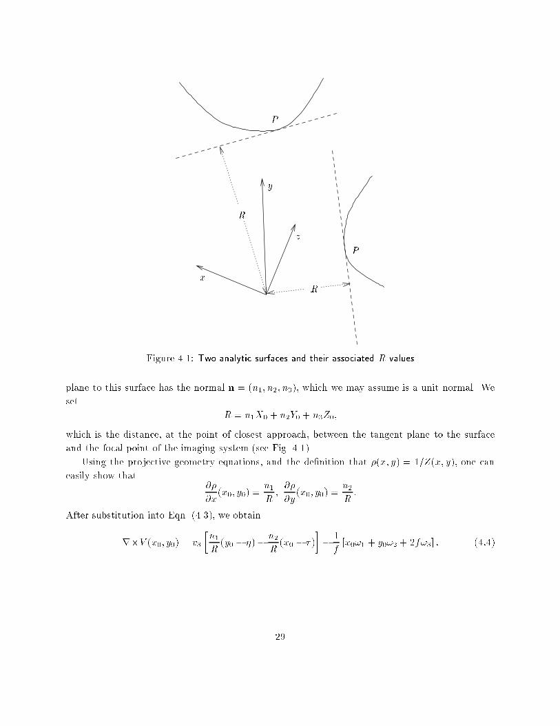
P
P
R
y
z
xR
Figure 4.1: Two analytic surfaces and their associated R values
plane to this surface has the normal n = (n1; n2; n3), which we may assume is a unit normal. We
set
R = n1X0 + n2Y0 + n3Z0;
which is the distance, at the point of closest approach, between the tangent plane to the surface
and the focal point of the imaging system (see Fig. 4.1).
Using the projective geometry equations, and the de�nition that �(x; y) = 1=Z(x; y), one can
easily show that@�
@x(x0; y0) =
n1R;@�
@y(x0; y0) =
n2R:
After substitution into Eqn. (4.3), we obtain
r�V (x0; y0) = v3
�n1R(y0 � �)�
n2R(x0 � �)
��
1
f[x0!1 + y0!2 + 2f!3] : (4:4)
29
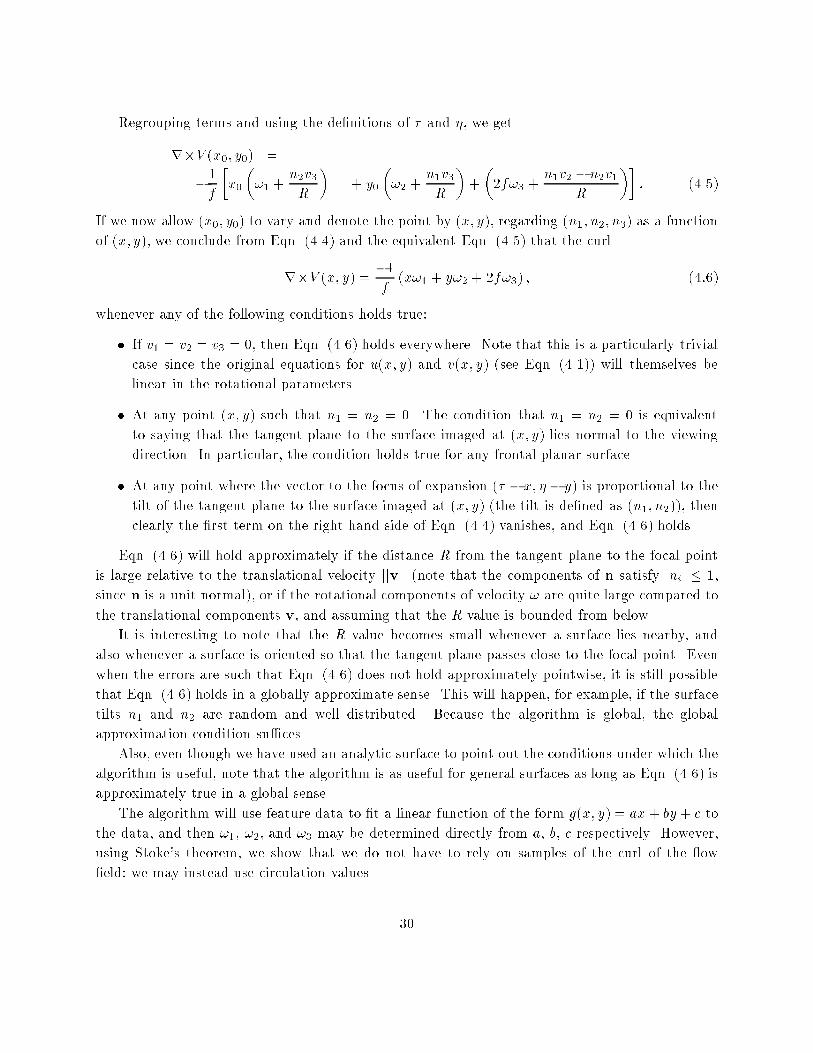
Regrouping terms and using the de�nitions of � and �, we get
r�V (x0; y0) =
�1
f
�x0
�!1 +
n2v3R
�+ y0
�!2 +
n1v3R
�+
�2f!3 +
n1v2 � n2v1R
��: (4.5)
If we now allow (x0; y0) to vary and denote the point by (x; y), regarding (n1; n2; n3) as a function
of (x; y), we conclude from Eqn. (4.4) and the equivalent Eqn. (4.5) that the curl
r�V (x; y) =�1
f(x!1 + y!2 + 2f!3) ; (4:6)
whenever any of the following conditions holds true:
� If v1 = v2 = v3 = 0, then Eqn. (4.6) holds everywhere. Note that this is a particularly trivial
case since the original equations for u(x; y) and v(x; y) (see Eqn. (4.1)) will themselves be
linear in the rotational parameters.
� At any point (x; y) such that n1 = n2 = 0. The condition that n1 = n2 = 0 is equivalent
to saying that the tangent plane to the surface imaged at (x; y) lies normal to the viewing
direction. In particular, the condition holds true for any frontal planar surface.
� At any point where the vector to the focus of expansion (� � x; � � y) is proportional to the
tilt of the tangent plane to the surface imaged at (x; y) (the tilt is de�ned as (n1; n2)), then
clearly the �rst term on the right hand side of Eqn. (4.4) vanishes, and Eqn. (4.6) holds.
Eqn. (4.6) will hold approximately if the distance R from the tangent plane to the focal point
is large relative to the translational velocity jjvjj (note that the components of n satisfy jnij � 1,
since n is a unit normal), or if the rotational components of velocity ! are quite large compared to
the translational components v, and assuming that the R value is bounded from below.
It is interesting to note that the R value becomes small whenever a surface lies nearby, and
also whenever a surface is oriented so that the tangent plane passes close to the focal point. Even
when the errors are such that Eqn. (4.6) does not hold approximately pointwise, it is still possible
that Eqn. (4.6) holds in a globally approximate sense. This will happen, for example, if the surface
tilts n1 and n2 are random and well distributed. Because the algorithm is global, the global
approximation condition su�ces.
Also, even though we have used an analytic surface to point out the conditions under which the
algorithm is useful, note that the algorithm is as useful for general surfaces as long as Eqn. (4.6) is
approximately true in a global sense.
The algorithm will use feature data to �t a linear function of the form g(x; y) = ax+ by + c to
the data, and then !1, !2, and !3 may be determined directly from a, b, c respectively. However,
using Stoke's theorem, we show that we do not have to rely on samples of the curl of the ow
�eld: we may instead use circulation values.
30
Figure 4.2: A collection of cycles and their centroids, where data for the ow circulation algorithm is
collected. The algorithm will simply �t a linear function to the circulation values given at each centroid.
Consider a region of the image domain D (not necessarily circular), such that at most of the
points (x; y) in D, one of the above conditions holds true. We do not require that D be a small
region, nor do we require that the same condition hold true over all of D, nor are we concerned
about substantial violations as long as the average of the violations is small. We will average the
values of the curl over D:1
jDj
Z ZD
r�V dx dy �1
jDj
Z ZD
�1
f[x!1 + y!2 + 2f!3]dx dy
= �1
f[x0!1 + y0!2 + 2f!3] ; (4.7)
where (x0; y0) is the centroid in the image plane of the region D. Here, jDj refers to the area of
D in the image domain. Applying Stoke's theorem to the left hand side of (4.7), we see that the
circulation value of V about the boundary of D satis�es
1
jDj
I@D
V � dS � �1
f[x0!1 + y0!2 + 2f!3] : (4:8)
4.4 The ow circulation algorithm
We now state the algorithm. Suppose we have a collection of image domains Di, i = 1; . . . ; N .
Suppose that we have normalized the circulation values measured for each such domain:
i =1
jDij
I@Di
V � ds:
Let us suppose that the centroid of each region Di is known, and is denoted by (xi; yi) (see Fig. 4.2).
From Eqn. (4.7), we know that the data (xi; yi; i), for i = 1; . . . ; N , satis�es, approximately,
i = axi + byi + c;
31
where a = �!1=f , b = �!2=f , and c = �2!3. We can determine the coe�cients a, b, and c by
�tting a linear function to the available data. Outliers, of course, can be discarded by standard
regression methods, so that violations of the conditions are not consequential. Clearly, the rotational
parameters are determined from a, b, and c.
If the collection of centroids of regions (xi; yi) is su�ciently dense and symmetrically distributed
about the image plane origin, then the determination of the rotational parameters from the cir-
culation data becomes especially simple, since then the parameters are coe�cients of mutually
orthogonal functions, Speci�cally, a will be proportional to the average value of xi � i, and b will
be proportional to the average value of yi � i, and c will be equal to the average value of i. Then
!1 = �fa, !2 = �fb, and !3 = �c=2. Once again, outliers may be discarded from the averages so
as to improve the quality of the estimates.
Thus, the algorithm simply involves computing contour integrals (which might be directly pro-
vided by feature detectors) and �tting a linear surface to this data.
32
Chapter 5
Translational parameter estimation
5.1 Introduction
The translation of a sensor, v = (v1; v2; v3), is an important quantity to be determined in visual
motion analysis. For instance, in navigation, it is important to determine the direction of movement
in order to avoid obstacles in the path. In turn, knowledge of the translation helps to determine
the scene structure and is useful in detecting obstacles. From monocular imagery, the translation
can be estimated only up to a scale factor, due to the combined e�ect of translation and depth
values on the ow �eld. One way to see this is to note that the same sequence can be produced by
a nearby point moving slowly or a distant point moving (proportionally) fast. This scale factor can
be absorbed into the unknown quantities in several ways. In particular, we will be interested in
determining the focus of expansion (FOE) which is nothing but the projection of the translational
velocity vector on the image plane.
The FOE is particularly easy to compute in the case where there is pure translation (i.e., zero
angular velocity). In such a case, the optical ow �eld is radially expanding or contracting, and the
FOE is found to be the point where the ow �eld vectors intersect. The simple-minded procedure
of �nding the FOE as the intersection point of the vectors does not work in practice for several
reasons. First, the optical ow �eld cannot be determined exactly, due to the aperture problem.
Secondly, noise adversely a�ects the ow �eld computation; and thirdly, pure translation is seldom
\pure" | there is always some rotation due to vibrations resulting in a turning of the camera
and other causes of rotation. Under such conditions, there is a need to somehow eliminate the
contribution from the rotation because the ow �eld is no longer of the radially expanding type.
Determination of the translation enables one to solve for the rotation and the structure of the
scene. Note that if the translation is known, then the optical ow equations become linear, and so
a collection of ow vectors provides enough information to solve for the other unknown quantities
using a linear algorithm. However, computation of the translation is made di�cult by the fact that
33
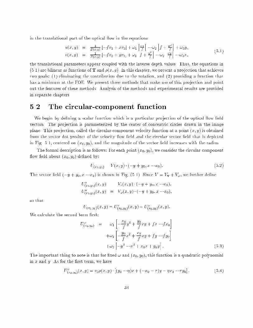
in the translational part of the optical ow in the equations
u(x; y) = 1Z(x;y) [�fv1 + xv3] + !1
hxyf
i� !2
hf + x2
f
i+ !3y;
v(x; y) = 1Z(x;y) [�fv2 + yv3] + !1
hf + y2
f
i� !2
hxyf
i� !3x;
(5:1)
the translational parameters appear coupled with the inverse depth values. Thus, the equations in
(5.1) are bilinear as functions of T and �(x; y). In this chapter, we present a projection that achieves
two goals: (1) eliminating the contribution due to the rotation, and (2) providing a function that
has a minimum at the FOE. We present three methods that make use of this projection and point
out the features of these methods. Analysis of the methods and experimental results are provided
in separate chapters.
5.2 The circular-component function
We begin by de�ning a scalar function which is a particular projection of the optical ow �eld
vectors. The projection is parameterized by the center of concentric circles drawn in the image
plane. This projection, called the circular-component velocity function at a point (x; y) is obtained
from the vector dot product of the velocity ow �eld and the circular vector �eld that is depicted
in Fig. 5.1, centered on (x0; y0), and the magnitude of the vector �eld increases with the radius.
The formal description is as follows: For each point (x0; y0), we consider the circular component
ow �eld about (x0; y0) de�ned by:
U(x0;y0) = V (x; y) � (�y + y0; x� x0): (5:2)
The vector �eld (�y + y0; x� x0) is shown in Fig. (5.1). Since V = Vv + V!, we further de�ne
Uv(x0;y0)
(x; y) = Vv(x; y) � (�y + y0; x� x0);
U!(x0;y0)
(x; y) = V!(x; y) � (�y + y0; x� x0);
so that
U(x0;y0)(x; y) = Uv(x0;y0)
(x; y) + U!(x0;y0)
(x; y):
We calculate the second term �rst:
U!(x0;y0)
= !1
��x0fy2 +
y0fxy + fx� fx0
�
+!2
��y0fx2 +
x0fxy + fy � fy0
�
+!3h�y2 � x2 + x0x+ y0y
i: (5.3)
The important thing to note is that for �xed ! and (x0; y0), this function is a quadratic polynomial
in x and y. As for the �rst term, we have
Uv(x0;y0)(x; y) = v3�(x; y) � [(y0 � �)x+ (�x0 + �)y + �x0 � �y0] : (5:4)
34
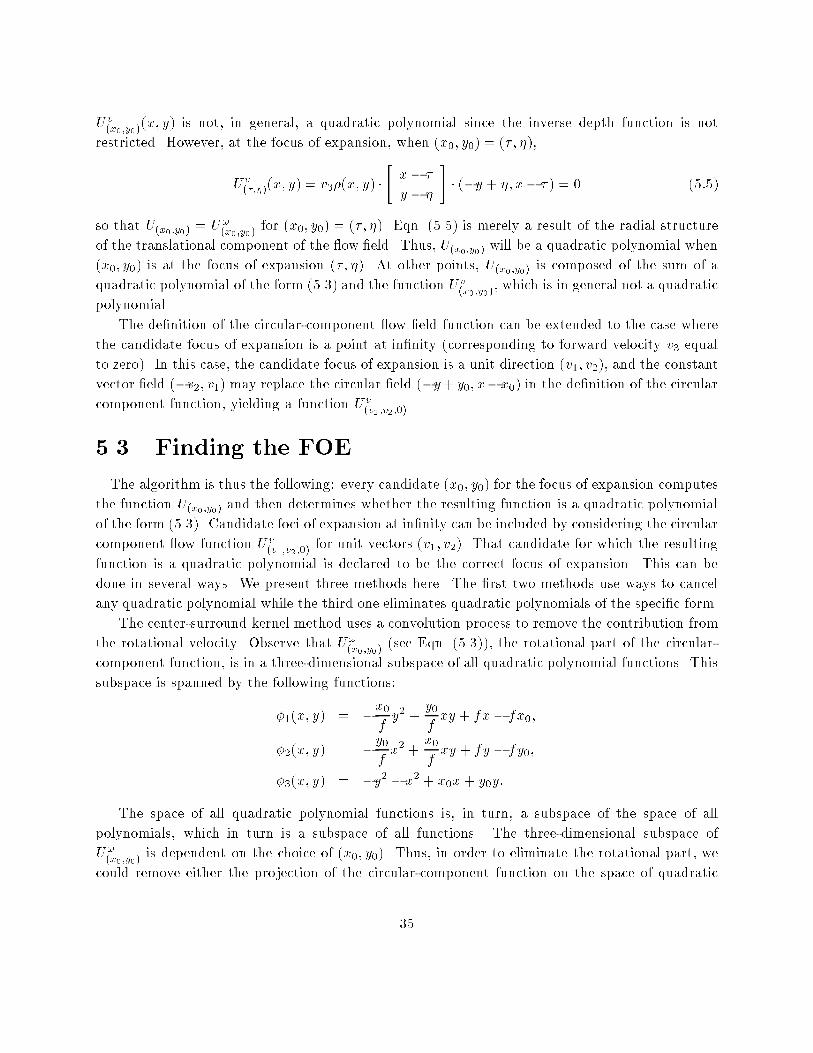
Uv(x0;y0)
(x; y) is not, in general, a quadratic polynomial since the inverse depth function is not
restricted. However, at the focus of expansion, when (x0; y0) = (�; �),
Uv(�;�)(x; y) = v3�(x; y) �
"x� �
y � �
#� (�y + �; x� �) = 0 (5:5)
so that U(x0;y0) = U!(x0;y0)
for (x0; y0) = (�; �). Eqn. (5.5) is merely a result of the radial structure
of the translational component of the ow �eld. Thus, U(x0;y0) will be a quadratic polynomial when
(x0; y0) is at the focus of expansion (�; �). At other points, U(x0;y0) is composed of the sum of a
quadratic polynomial of the form (5.3) and the function Uv(x0;y0)
, which is in general not a quadratic
polynomial.
The de�nition of the circular-component ow �eld function can be extended to the case where
the candidate focus of expansion is a point at in�nity (corresponding to forward velocity v3 equal
to zero). In this case, the candidate focus of expansion is a unit direction (v1; v2), and the constant
vector �eld (�v2; v1) may replace the circular �eld (�y+ y0; x�x0) in the de�nition of the circular
component function, yielding a function Uv(v1;v2;0)
.
5.3 Finding the FOE
The algorithm is thus the following: every candidate (x0; y0) for the focus of expansion computes
the function U(x0;y0) and then determines whether the resulting function is a quadratic polynomial
of the form (5.3). Candidate foci of expansion at in�nity can be included by considering the circular
component ow function Uv(v1;v2 ;0)
for unit vectors (v1; v2). That candidate for which the resulting
function is a quadratic polynomial is declared to be the correct focus of expansion. This can be
done in several ways. We present three methods here. The �rst two methods use ways to cancel
any quadratic polynomial while the third one eliminates quadratic polynomials of the speci�c form.
The center-surround kernel method uses a convolution process to remove the contribution from
the rotational velocity. Observe that U!(x0;y0)
(see Eqn. (5.3)), the rotational part of the circular-
component function, is in a three-dimensional subspace of all quadratic polynomial functions. This
subspace is spanned by the following functions:
�1(x; y) = �x0fy2 +
y0fxy + fx� fx0;
�2(x; y) = �y0fx2 +
x0fxy + fy � fy0;
�3(x; y) = �y2 � x2 + x0x+ y0y:
The space of all quadratic polynomial functions is, in turn, a subspace of the space of all
polynomials, which in turn is a subspace of all functions. The three-dimensional subspace of
U!(x0;y0)
is dependent on the choice of (x0; y0). Thus, in order to eliminate the rotational part, we
could remove either the projection of the circular-component function on the space of quadratic
35
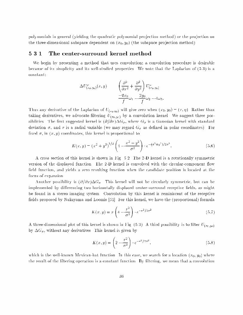
polynomials in general (yielding the quadratic polynomial projection method) or the projection on
the three-dimensional subspace dependent on (x0; y0) (the subspace projection method).
5.3.1 The center-surround kernel method
We begin by presenting a method that uses convolution; a convolution procedure is desirable
because of its simplicity and its well-studied properties. We note that the Laplacian of (5.3) is a
constant:
�U!(x0;y0)
(x; y) =
@2
@x2+
@2
@y2
!U!(x0;y0)
=�2x0f
!1 � 2y0f!2 � 4!3:
Thus any derivative of the Laplacian of U(x0;y0) will give zero when (x0; y0) = (�; �). Rather than
taking derivatives, we advocate �ltering U(x0;y0) by a convolution kernel. We suggest three pos-
sibilities. The �rst suggested kernel is (@=@r)�G�, where G� is a Gaussian kernel with standard
deviation �, and r is a radial variable (we may regard G� as de�ned in polar coordinates). For
�xed �, in (x; y) coordinates, this kernel is proportional to
K(x; y) = (x2 + y2)1=2
4� x2 + y2
�2
!� e�(x2+y2)=2�2 : (5:6)
A cross section of this kernel is shown in Fig. 5.2. The 2-D kernel is a rotationally symmetric
version of the displayed function. The 2-D kernel is convolved with the circular-component ow
�eld function, and yields a zero resulting function when the candidate position is located at the
focus of expansion.
Another possibility is (@=@x)�G�. This kernel will not be circularly symmetric, but can be
implemented by di�erencing two horizontally displaced center-surround receptive �elds, as might
be found in a stereo imaging system. Convolution by this kernel is reminiscent of the receptive
�elds proposed by Nakayama and Loomis [51]. For this kernel, we have the (proportional) formula
K(x; y) = x
4� r2
�2
!� e�r2=2�2 (5:7)
A three-dimensional plot of this kernel is shown in Fig. (5.3). A third possibility is to �lter U(x0;y0)
by �G�, without any derivatives. This kernel is given by
K(x; y) =
2� r2
�2
!� e�r2=2�2 ; (5:8)
which is the well-known Mexican-hat function. In this case, we search for a location (x0; y0) where
the result of the �ltering operation is a constant function. By �ltering, we mean that a convolution
36
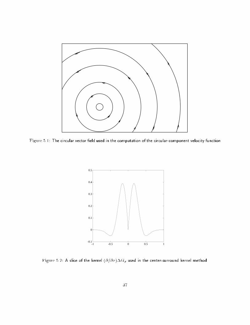
Figure 5.1: The circular vector �eld used in the computation of the circular-component velocity function
-0.1
0
0.1
0.2
0.3
0.4
0.5
-1 -0.5 0 0.5 1
Figure 5.2: A slice of the kernel (@=@r)�G� used in the center-surround kernel method.
37
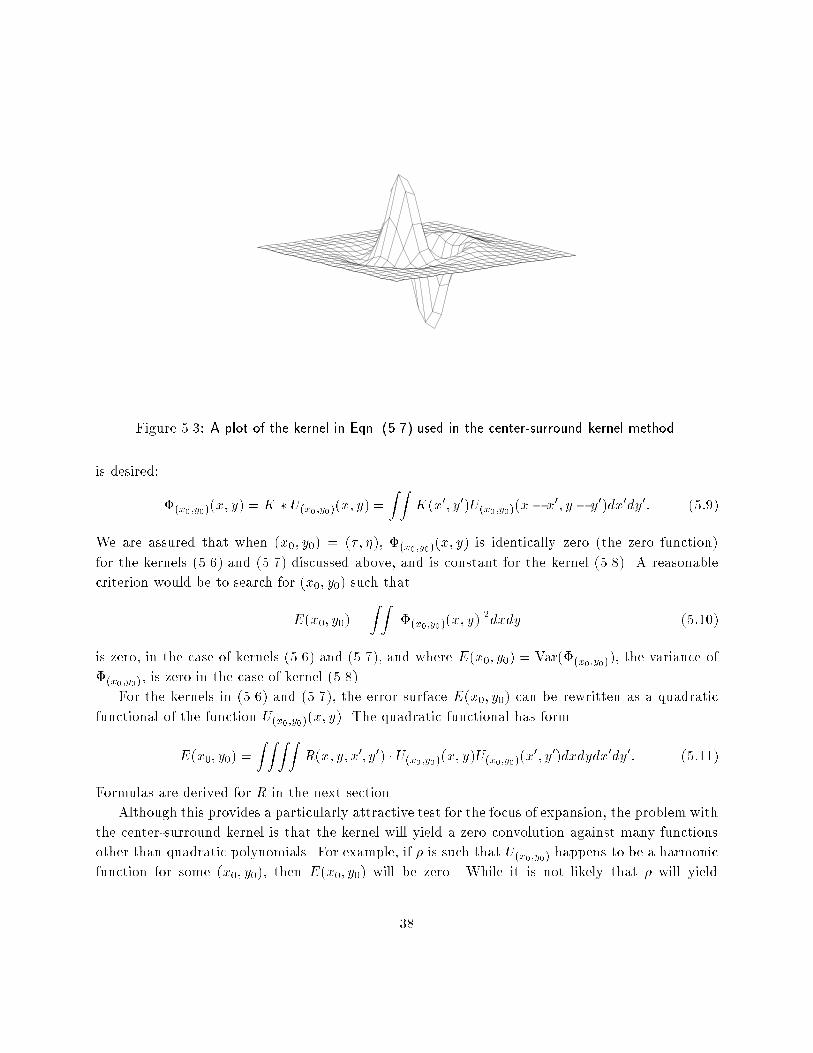
Figure 5.3: A plot of the kernel in Eqn. (5.7) used in the center-surround kernel method.
is desired:
�(x0;y0)(x; y) = K � U(x0;y0)(x; y) =Z Z
K(x0; y0)U(x0;y0)(x� x0; y � y0)dx0dy0: (5:9)
We are assured that when (x0; y0) = (�; �), �(x0;y0)(x; y) is identically zero (the zero function)
for the kernels (5.6) and (5.7) discussed above, and is constant for the kernel (5.8). A reasonable
criterion would be to search for (x0; y0) such that
E(x0; y0) =
Z Zj�(x0;y0)(x; y)j2dxdy (5:10)
is zero, in the case of kernels (5.6) and (5.7), and where E(x0; y0) = Var(�(x0;y0)), the variance of
�(x0;y0), is zero in the case of kernel (5.8).
For the kernels in (5.6) and (5.7), the error surface E(x0; y0) can be rewritten as a quadratic
functional of the function U(x0;y0)(x; y). The quadratic functional has form
E(x0; y0) =Z Z Z Z
R(x; y; x0; y0) �U(x0;y0)(x; y)U(x0;y0)(x0; y0)dxdydx0dy0: (5:11)
Formulas are derived for R in the next section.
Although this provides a particularly attractive test for the focus of expansion, the problem with
the center-surround kernel is that the kernel will yield a zero convolution against many functions
other than quadratic polynomials. For example, if � is such that U(x0;y0) happens to be a harmonic
function for some (x0; y0), then E(x0; y0) will be zero. While it is not likely that � will yield
38
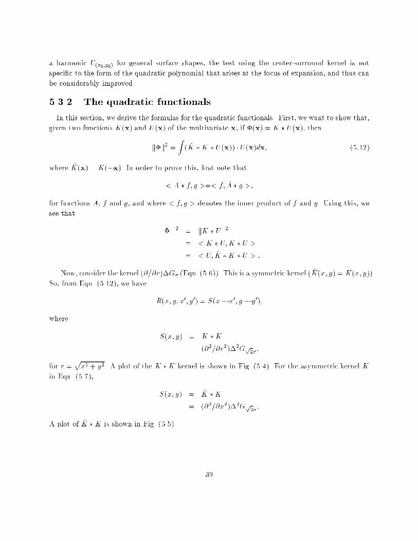
a harmonic U(x0;y0) for general surface shapes, the test using the center-surround kernel is not
speci�c to the form of the quadratic polynomial that arises at the focus of expansion, and thus can
be considerably improved.
5.3.2 The quadratic functionals
In this section, we derive the formulas for the quadratic functionals. First, we want to show that,
given two functions K(x) and U(x) of the multivariate x, if �(x) = K �U(x), then
k�k2 =Z( �K �K � U(x)) � U(x)dx; (5:12)
where �K(x) = K(�x). In order to prove this, �rst note that
< A � f; g >=< f; �A � g >;
for functions A, f and g, and where < f; g > denotes the inner product of f and g. Using this, we
see that
k � k2 = kK �Uk2= < K � U;K � U >
= < U; �K �K � U > :
Now, consider the kernel (@=@r)�G� (Eqn. (5.6)). This is a symmetric kernel ( �K(x; y) = K(x; y)).
So, from Eqn. (5.12), we have
R(x; y; x0; y0) = S(x� x0; y � y0);
where
S(x; y) = K �K= (@2=@r2)�2Gp
2�;
for r =px2 + y2. A plot of the K �K kernel is shown in Fig. (5.4). For the asymmetric kernel K
in Eqn. (5.7),
S(x; y) = �K �K= (@2=@x2)�2Gp
2�:
A plot of �K �K is shown in Fig. (5.5).
39
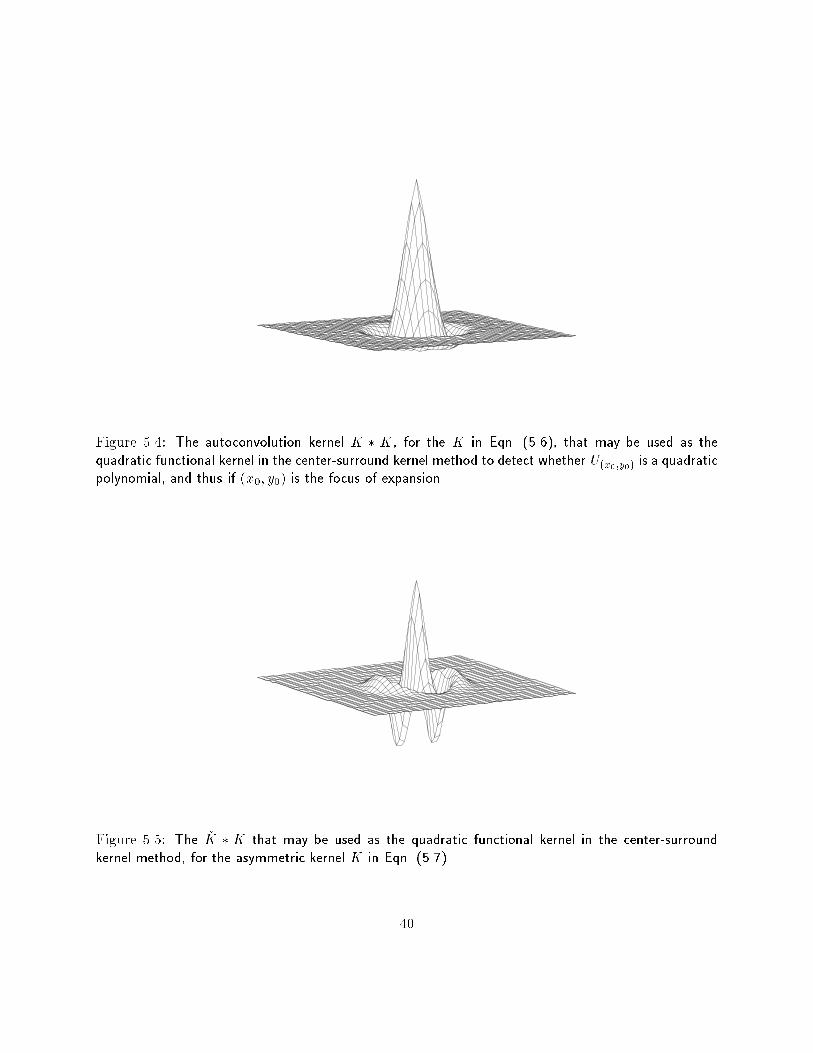
Figure 5.4: The autoconvolution kernel K � K, for the K in Eqn. (5.6), that may be used as thequadratic functional kernel in the center-surround kernel method to detect whether U(x0;y0) is a quadraticpolynomial, and thus if (x0; y0) is the focus of expansion.
Figure 5.5: The �K � K that may be used as the quadratic functional kernel in the center-surroundkernel method, for the asymmetric kernel K in Eqn. (5.7).
40
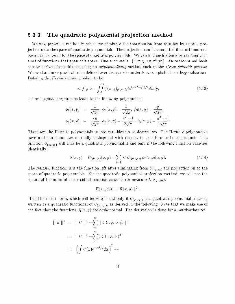
5.3.3 The quadratic polynomial projection method
We now present a method in which we eliminate the contribution from rotation by using a pro-
jection onto the space of quadratic polynomials. The projection can be computed if an orthonormal
basis can be found for the space of quadratic polynomials. We can �nd such a basis by starting with
a set of functions that span this space. One such set is: f1; x; y; xy; x2; y2g. An orthonormal basis
can be derived from this set using an orthogonalizing method such as the Gram-Schmidt process.
We need an inner product to be de�ned over the space in order to accomplish the orthogonalization.
De�ning the Hermite inner product to be
< f; g >=
Z Zf(x; y)g(x; y)e(�x
2�y2)=2dxdy; (5:13)
the orthogonalizing process leads to the following polynomials:
�1(x; y) =1p2�
; �2(x; y) =xp2�
; �3(x; y) =yp2�
;
�4(x; y) =xyp2�
; �5(x; y) =x2 � 1
2p�; �6(x; y) =
y2 � 1
2p�:
These are the Hermite polynomials in two variables up to degree two. The Hermite polynomials
have unit norm and are mutually orthogonal with respect to the Hermite inner product. The
function U(x0;y0) will thus be a quadratic polynomial if and only if the following function vanishes
identically:
(x; y) = U(x0;y0)(x; y)�6X
i=1
< U(x0;y0); �i > �i(x; y): (5:14)
The residual function is the function left after eliminating from U(x0;y0) the projection on to the
space of quadratic polynomials. For the quadratic polynomial projection method, we will use the
square of the norm of this residual function as our error measure E(x0; y0):
E(x0; y0) =k (x; y) k2 :
The (Hermite) norm, which will be zero if and only if U(x0;y0) is a quadratic polynomial, may be
written as a quadratic functional of U(x0;y0), as derived in the following. Note that we make use of
the fact that the functions �i(x; y) are orthonormal. The derivation is done for a multivariate x:
k k2 = k U k2 �6X
i=1
k< U; �i > �i k2
= k U k2 �6X
i=1
(< U; �i >)2
=
�ZU(x)e�x
2=2dx
�2�
41
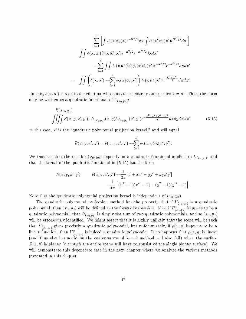
6Xi=1
�ZU(x)�i(x)e
�x2=2dxZU(x0)�i(x
0)ex02=2dx0
�
=Z Z
�(x;x0)U(x)U(x0)e�x2=2e�x
02=2dxdx0
�6X
i=1
Z ZU(x)U(x0)�i(x)�i(x
0)e�x2=2e�x
02=2dxdx0
=
Z Z �(x;x0)�
6Xi=1
�i(x)�i(x0)
!U(x)U(x0)e�
x2+x
02
2 dxdx0:
In this, �(x;x0) is a delta distribution whose mass lies entirely on the slice x = x0. Thus, the norm
may be written as a quadratic functional of U(x0;y0):
E(x0; y0) =ZZZZR(x; y; x0; y0) � U(x0;y0)(x; y)U(x0;y0)(x
0; y0)e�x2+y
2+x
02+y
02
2 dxdydx0dy0: (5.15)
In this case, R is the \quadratic polynomial projection kernel," and will equal
R(x; y; x0; y0) = �(x; y; x0; y0)�6X
i=1
�i(x; y)�i(x0; y0):
We thus see that the test for (x0; y0) depends on a quadratic functional applied to U(x0;y0), and
that the kernel of the quadratic functional in (5.15) has the form
R(x; y; x0; y0) = �(x; y; x0; y0)� 1
2�
�1 + xx0 + yy0 + xyx0y0
�� 1
4�
h(x2 � 1)(x02� 1) + (y2 � 1)(y02 � 1)
i:
Note that the quadratic polynomial projection kernel is independent of (x0; y0).
The quadratic polynomial projection method has the property that if U(x0;y0) is a quadratic
polynomial, then (x0; y0) will be de�ned as the focus of expansion. Alas, if Uv(x0;y0)
happens to be a
quadratic polynomial, then U(x0;y0) is simply the sum of two quadratic polynomials, and so (x0; y0)
will be erroneously identi�ed. We might assert that it is highly unlikely that the scene will be such
that Uv(x0;y0)
gives precisely a quadratic polynomial, but unfortunately, if �(x; y) happens to be a
linear function, then Uv(x0;y0)
is indeed a quadratic polynomial. It so happens that �(x; y) is linear
(and thus also harmonic, so the center-surround kernel method will also fail) when the surface
Z(x; y) is planar (although the entire scene will have to consist of the single planar surface). We
will demonstrate this degenerate case in the next chapter where we analyze the various methods
presented in this chapter.
42
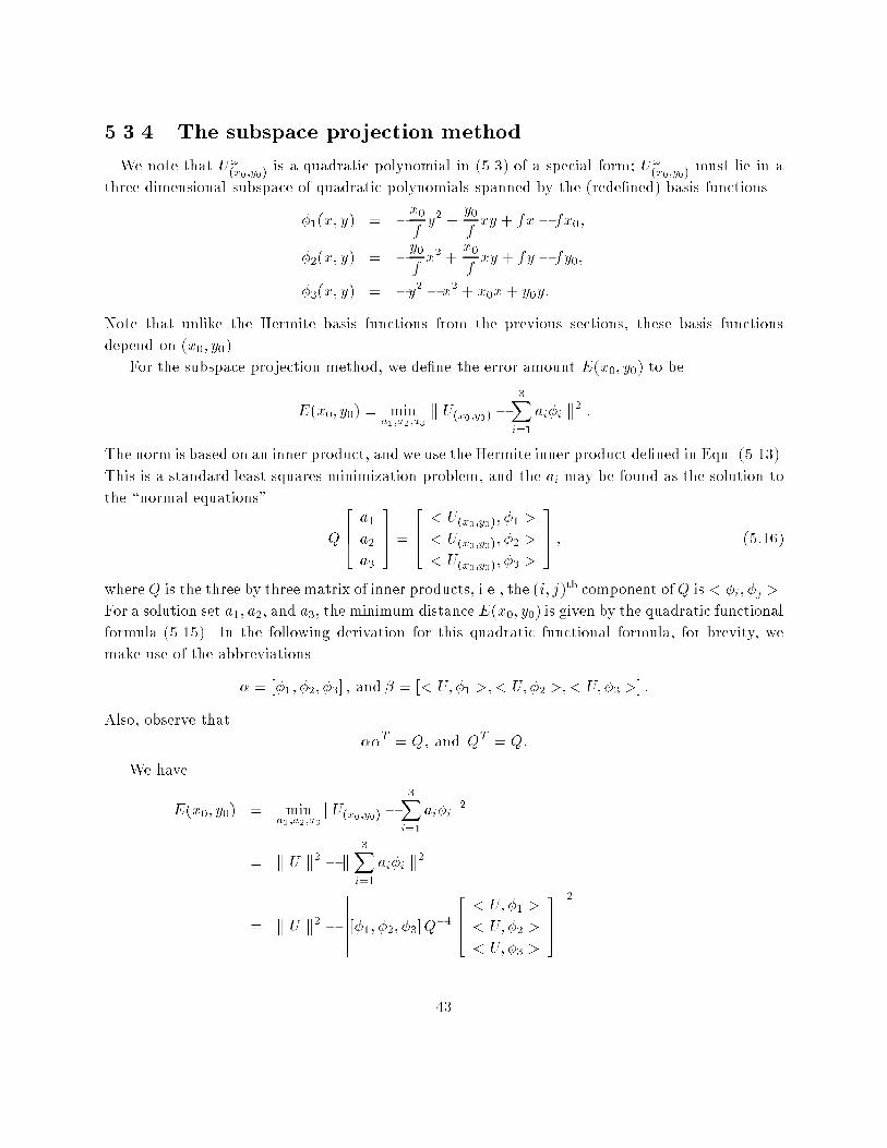
5.3.4 The subspace projection method
We note that U!(x0;y0)
is a quadratic polynomial in (5.3) of a special form; U!(x0;y0)
must lie in a
three dimensional subspace of quadratic polynomials spanned by the (rede�ned) basis functions
�1(x; y) = �x0fy2 +
y0fxy + fx� fx0;
�2(x; y) = �y0fx2 +
x0fxy + fy � fy0;
�3(x; y) = �y2 � x2 + x0x+ y0y:
Note that unlike the Hermite basis functions from the previous sections, these basis functions
depend on (x0; y0).
For the subspace projection method, we de�ne the error amount E(x0; y0) to be
E(x0; y0) = mina1;a2;a3
k U(x0;y0) �3X
i=1
ai�i k2 :
The norm is based on an inner product, and we use the Hermite inner product de�ned in Eqn. (5.13).
This is a standard least squares minimization problem, and the ai may be found as the solution to
the \normal equations"
Q
264a1a2a3
375 =
264< U(x0;y0); �1 >
< U(x0;y0); �2 >
< U(x0;y0); �3 >
375 ; (5:16)
where Q is the three by three matrix of inner products, i.e., the (i; j)th component ofQ is < �i; �j >.
For a solution set a1; a2, and a3, the minimum distance E(x0; y0) is given by the quadratic functional
formula (5.15). In the following derivation for this quadratic functional formula, for brevity, we
make use of the abbreviations
� = [�1; �2; �3] ; and � = [< U; �1 >;< U; �2 >;< U; �3 >] :
Also, observe that
��T = Q; and QT = Q:
We have
E(x0; y0) = mina1;a2;a3
kU(x0;y0) �3X
i=1
ai�ik2
= k U k2 � k3X
i=1
ai�i k2
= k U k2 �
��������������[�1; �2; �3]Q
�1
264< U; �1 >
< U; �2 >
< U; �3 >
375��������������2
43
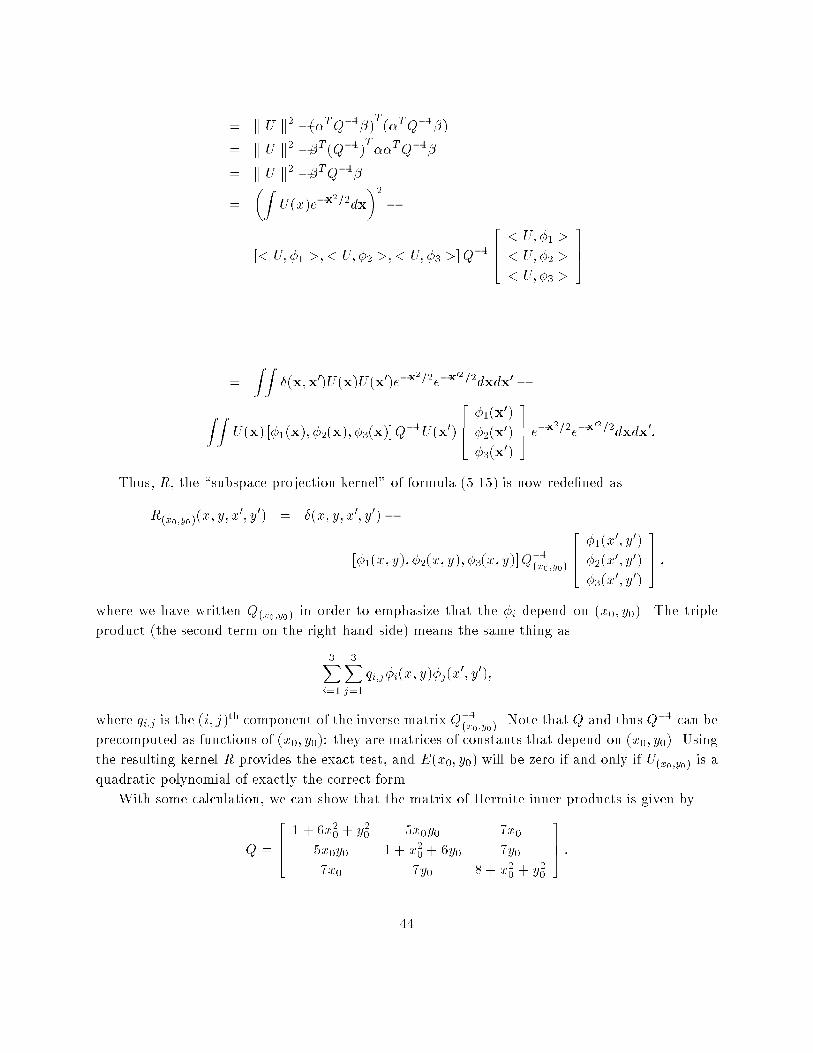
= k U k2 �(�TQ�1�)T(�TQ�1�)
= k U k2 ��T (Q�1)T��TQ�1�
= k U k2 ��TQ�1�
=
�ZU(x)e�x
2=2dx
�2�
[< U; �1 >;< U; �2 >;< U; �3 >]Q�1
264< U; �1 >
< U; �2 >
< U; �3 >
375
=Z Z
�(x;x0)U(x)U(x0)e�x2=2e�x
02=2dxdx0�
Z ZU(x) [�1(x); �2(x); �3(x)]Q
�1U(x0)
264�1(x0)�2(x0)�3(x0)
375 e�x2=2e�x02=2dxdx0:
Thus, R, the \subspace projection kernel" of formula (5.15) is now rede�ned as
R(x0;y0)(x; y; x0; y0) = �(x; y; x0; y0)�
[�1(x; y); �2(x; y); �3(x; y)]Q�1(x0;y0)
264�1(x
0; y0)�2(x
0; y0)�3(x0; y0)
375 ;
where we have written Q(x0;y0) in order to emphasize that the �i depend on (x0; y0). The triple
product (the second term on the right hand side) means the same thing as
3Xi=1
3Xj=1
qi;j�i(x; y)�j(x0; y0);
where qi;j is the (i; j)th component of the inverse matrix Q�1(x0;y0)
. Note that Q and thus Q�1 can beprecomputed as functions of (x0; y0): they are matrices of constants that depend on (x0; y0). Using
the resulting kernel R provides the exact test, and E(x0; y0) will be zero if and only if U(x0;y0) is a
quadratic polynomial of exactly the correct form.
With some calculation, we can show that the matrix of Hermite inner products is given by
Q =
2641 + 6x20 + y20 5x0y0 7x0
5x0y0 1 + x20 + 6y0 7y07x0 7y0 8 + x20 + y20
375 :
44
We discover that an inverse always exists, and that the coe�cients are quotients of sixth order
polynomials (i.e., rational polynomials) in the two position values. These functions do not have to
be solved! They are merely evaluated for each (x0; y0) that is considered. The nine values qi;j of
the inverse matrix Q�1 can be computed for each (x0; y0) using the following formulas:
q1;1 = (8 + 9x20 + 7x20y20 + x40 + 6y40)=P;
q2;2 = (8 + 9y20 + 7x20y20 + 6x40 + y40)=P;
q3;3 = (1 + 7(x20 + y20) + 6(x40 + y40) + 12x20y20)=P;
q1;2 = (�5x30y0 � 5x0y30 + 9x0y0)=P;
q1;3 = �7x0(1 + x20 + y20)=P;
q2;3 = �7y0(1 + y20 + x20)=P;
(5:17)
where
P = det(Q) = 8 + 8(x20 + y20) + 12x20y20 + 6(x40 + y40) + 18(x20y
40 + x40y
20) + 6(x60 + y60);
and
q3;2 = q2;3; q1;2 = q2;1; q1;3 = q3;1: (5:18)
To summarize, the task for any given point (x0; y0) is to compute the function U(x0;y0) using
(5.2) and the values of qi;j using (5.17) and (5.18), and to use these values to compose the quadratic
functional kernel, and then to compute the value of the quadratic functional applied to the function
U(x0;y0) using (5.11). The result will be zero if (x0; y0) is at the focus of expansion.
In the methods presented so far, there are two ways to compute the error surface value E(x0; y0)
from U(x0;y0)(x; y). One way is to convolve with a kernel (center-surround kernel method) or, to
compute an explicit projection on a subspace (quadratic polynomial projection method, subspace
projection method) and then to eliminate this projection from U(x0;y0)(x; y); the norm of the func-
tion left after this operation is the error surface value. The second way is to calculate the quadratic
functional kernel R(x; y; x0; y0) and then to directly compute the error value by doing a quadratic
functional computation in the four dimensional space of (x; y; x0; y0), as shown in Eqn. (5.15). If
there are n points in the discrete domain where the ow values are known, the latter method in-
volving a quadratic functional kernel is of complexity O(n2) and the former method is of complexity
O(n).
5.4 The quadratic error surface result
It will be shown that the error function E(x0; y0) in the case of the center-surround kernel method
and the quadratic polynomial projection method is itself a quadratic polynomial. The implication
of such a result is that one does not have to search over all possible candidate FOEs in order to
determine the minimum of the error function. Indeed, there is no need for a minimization procedure,
either. Given the values of the function E(x0; y0) at six points, the function E(x0; y0) is completely
45
determined because of its quadratic nature. The coe�cients of the quadratic polynomial can be
found from the values at the six points and the minimum of the function can be expressed in closed
form in terms of these coe�cients.
5.4.1 The center-surround kernel method
For the center-surround kernel method, the function E(x0; y0) is obtained by a convolution
process. Note �rst that the function U(x0;y0)(x; y) is linear in x0 and y0:
U(x0;y0)(x; y) = V (x; y) � (�y + y0; x� x0):
Let us make explicit the linearity in (x0; y0):
U(x0;y0)(x; y) = A(x; y)x0+ B(x; y)y0 + C(x; y); (5:19)
where the functions A(x; y), B(x; y) and C(x; y) will depend on the ow �eld V (x; y). The convo-
lution kernel K, which is also a function of x and y, is independent of (x0; y0). So, when U(x0;y0) is
convolved with K, the resulting function �(x0;y0) is still linear in x0 and y0:
�(x0;y0)(x; y) = U(x0;y0) �K(x; y)
= (A �K(x; y))x0+ (B �K(x; y))y0+ (C �K(x; y))
= A1(x; y)x0+B1(x; y)y0+ C1(x; y);
where A1(x; y), B1(x; y) and C1(x; y) are respectively, the results of the convolution of A(x; y),
B(x; y) and C(x; y) with the kernel K(x; y). The form of �(x0;y0) is seen to be linear in x0 and
y0. Note that this observation does not depend on the choice of K, as long as K is independent of
(x0; y0). The error function E(x0; y0) is de�ned to be the norm square of �(x0;y0) (see Eqn. (5.10)):
E(x0; y0) =k �(x0;y0)(x; y) k2 :Since we know that �(x0;y0) is linear in x0 and y0, we can show that E(x0; y0) is quadratic in x0and y0. In the following, for simplicity, we do not show the dependence on x and y.
E(x0; y0) = k �(x0;y0) k2
=
Z Z[A1x0 +B1y0 + C1]
2 dxdy
= kA1k2 x20+ kB1 k2 y20 + 2 kA1B1 k x0y0 + 2 kA1C1k x0+2 kB1C1k y0+ kC1k2 : (5.20)
For the variance case,
E(x0; y0) =Z Z
(�(x0;y0) � �a(x0;y0)
)2dxdy (5:21)
Here �a(x0;y0)
is the mean value of the function �(x0;y0), and is also linear in x0 and y0. Thus the
expression inside the integral in Eqn. 5.21 is linear in x0 and y0. By a development similar to the
one in Eqn. (5.20), the error function is quadratic in this case also.
Thus, E(x0; y0) is a quadratic polynomial in x0 and y0, for the center-surround kernel method.
46
5.4.2 The quadratic polynomial projection method
For the quadratic polynomial projection method, the error function E(x0; y0) is obtained as the
norm of the orthogonal complement function which is the residual left after subtracting o� the
projection on to the space of quadratic polynomials. That is, E(x0; y0) is the norm of the following
function reproduced from Eqn. (5.14):
�(x; y) = U(x0;y0)(x; y)�6X
i=1
< U(x0;y0); �i > �i(x; y):
The function U(x0;y0)(x; y) is linear in x0 and y0 (see Eqn. (5.19). We have noted that the basis
functions �i that span the space of quadratic polynomials are independent of x0 and y0. This means
that the projections
< U(x0;y0); �i > �i(x; y) = < A; �i > x0�i(x; y)+ < B; �i > y0�i(x; y)
+ < C; �i > �i(x; y)
are linear functions of x0 and y0. Here, we have used the linearity of the inner product. Continuing,
we see that the summation6X
i=1
< U(x0;y0); �i > �i(x; y)
and so the orthogonal complement
�(x; y) = U(x0;y0)(x; y)�6X
i=1
< U(x0;y0); �i > �i(x; y)
are also linear functions of x0 and y0. As a result the error, which is the norm square of the function
�(x; y), is quadratic in x0 and y0, as shown for the center-surround kernel method in Eqn. (5.20).
5.4.3 Invariance under noise
It can be easily seen that additive noise will contribute another linear term to the functions; thus,
the error function would still be quadratic. Let N(x; y) represent the additive noise in the optical
ow computation. We replace V (x; y) by V (x; y)+N(x; y) in the equations involving V (x; y). The
circular-component function for this noisy ow �eld is
U(x0;y0)(x; y) = (V (x; y) +N(x; y)) � (�y + y0; x� x0):
The function U(x0;y0)(x; y) still remains linear in x0 and y0. Thus, the reasoning for the quadratic
nature of the error function E(x0; y0) would still carry through as in the noiseless case. In general,
the vector ow �eld V (x; y) in the de�nition of the circular-component function can be replaced
by any arbitrary vector �eld (in particular, such a ow �eld can be produced by an arbitrary
47
transformation of the optical ow �eld); but the error function E(x0; y0) would still be quadratic
in x0 and y0 by means of the same arguments we presented so far. However, the minimum of the
quadratic surface need no longer be at the correct FOE. Indeed, in general, the minimum would
occur at a location di�erent from the correct FOE because of the transformation brought upon
V (x; y). Even though the nature of the surface remains quadratic, the minimum value need no
longer be zero. The departure of the minimum value from zero is a measure of the noise in the ow
�eld.
5.4.4 Using the quadratic error surface result
So, the algorithm in both the center-surround kernel method and the quadratic polynomial
projection method is as follows: Choose six locations (x0i; y0i). The choice of the locations is
immaterial, and could be done at random, as long as they are in a non-degenerate con�guration.
For each (x0i; y0i), compute the error function E(x0i; y0i) by convolving or projecting the circular
component U(x0;y0)(x; y) (depending on which method is used) and then taking the norm of the
resulting function. Fit a quadratic surface to these six values of E. The quadratic surface is of the
form
E(x0i; y0i) = a1x20i + a2y
20i + a3x0iy0i + a4x0i + a5y0i + a6:
Since we know the value of E for six (x0i; y0i), we get six linear equations in the six unknowns aj ,
1�j�6. This linear system can be solved using standard techniques. Of course, one could choose
a speci�c set of six points (x0i; y0i) in advance and precompute the inverse matrix required in the
linear system solution.
The minimum of this quadratic surface E, which is the FOE, can be easily determined as a
closed-form function of the parameters of the quadratic surface. The minimum of the surface is
located at �2a1a5 � a3a4a23 � 4a1a2
;2a2a4 � a3a5a23 � 4a1a2
�:
as can be seen by solving for that (x0i; y0i) for which
@E
@x0i= 0; and
@E
@y0i= 0:
Note that the coe�cients aj are determined from the values of E at six points by solving a linear
system of equations. In this sense, no search is involved in the center-surround kernel and the
quadratic polynomial projection methods. However, the error surface in the third method (the
subspace projection method) does not have the quadratic nature because the projection itself
depends on the values of x0i and y0i. So, in this case, a good strategy for locating the minimum
would be of advantage.
Note that obtaining the values of E at more than six points is redundant. This is so because
the quadratic error surface is perfectly quadratic, irrespective of the input ow �eld. So, no gain is
achieved by computing the value of E at more than six points.
48
5.5 A fast method: the NCC algorithm
In this section, we present a variation of the FOE search algorithm that o�ers certain compu-
tational advantages over the previous algorithms. In certain circumstances, the method performs
better. This method is an approximate method in that it requires that the rotational parameters
be small. We want to ignore the part of the ow �eld resulting from the rotational motion. In
other words, we require that the translational motion dominate. Then we can avoid doing one of
the steps (that of eliminating the contribution to the ow �eld by the rotational velocity) in the
previous methods. The result is a faster algorithm (compared to the ones presented so far) that
does very well under pure or nearly-pure translational motion. In most real-life motion there is
hardly any rotation; the fast method we present here will be useful under such conditions.
The circular component function is composed of two parts, one (Uv(x0;y0)
) from the translational
velocity, and the other (U!(x0;y0)
) due to the rotational velocity:
U(x0;y0)(x; y) = Uv(x0;y0)
(x; y) + U!(x0;y0)
(x; y):
Recall that all the FOE search methods described so far try to eliminate U!(x0;y0)
by either convolv-
ing with a kernel (center-surround kernel method) or by projecting on to a subspace (quadratic
polynomial projection method, subspace projection method). Here we consider the option of ig-
noring the step of eliminating U!(x0;y0)
. To this end, we de�ne an error function E(x0; y0) as the
norm of U(x0;y0)(x; y):
E(x0; y0) = kU(x0;y0)k2: (5:22)
The important observation, as noted before, is that U(x0;y0)(x; y) is linear in the parameters x0 and
y0:
U(x0;y0)(x; y) = V (x; y) � (�y + y0; x� x0);
or, more explicitly,
U(x0;y0)(x; y) = A(x; y)x0+ B(x; y)y0 + C(x; y);
where the functions A(x; y), B(x; y) and C(x; y) will depend on the ow �eld V (x; y). The norm
of U(x0;y0)(x; y) as shown in Eqn. (5.22) gives an error function
E(x0; y0) = k U(x0;y0)(x0; y0) k2
=
Z Z[Ax0 +By0 + C]2 dxdy
= k A k2 x20+ k B k2 y20 + 2 k AB k x0y0+2 k AC k x0 + 2 k BC k y0+ k C k2 :
Thus the error function de�ned in Eqn. (5.22) is quadratic in x0 and y0. The minimum of this
quadratic surface is purported to occur at the Focus of Expansion (FOE). We will justify this claim
49
shortly. But �rst, if the claim is correct, we have a simple procedure [67] { the Norm of the Circular
Component (NCC) algorithm { that we describe now.
The �rst step is to choose six candidate coordinate positions (x0i; y0i) in a non-degenerate
con�guration (i.e., six points on the image plane that are not on a straight line). Next, for each of
these candidates, compute the circular component function and de�ne E(x0i; y0i) to be the norm
of that function. In a discrete setting, the error value is simply the sum of the squares of the
circular component values. Note that this can be done even in the case of a sparse ow �eld. The
error function values at these six points completely de�ne the error surface because of its quadratic
nature. If we write the error surface to be
E(x0i; y0i) = a1x20i + a2y
20i + a3x0iy0i + a4x0i + a5y0i + a6;
we can solve for the unknowns aj ; 1�j�6, given the error values for the six candidates (x0i; y0i); 1�i� 6, by solving a system of six linear equations in six unknowns. The location of the minimum
can be found using the closed-form expression�2a1a5 � a3a4a23 � 4a1a2
;2a2a4 � a3a5a23 � 4a1a2
�;
as shown in the previous section. This location is the computed FOE. Thus the algorithm involves
computing the norm of the circular component function for six candidates, calculating the param-
eters of the quadratic error surface by solving a linear system, and then computing the FOE using
a closed form expression.
Let us now examine the claim about the minimum being at the the FOE. Note that the function
U(x0;y0)(x; y) is made up of two parts; one is the translational part shown in Eqn. (5.4), and the
other is the rotational, in (Eqn. (5.3)):
Uv(x0;y0)
(x; y) = v3�(x; y) � [(y0 � �)x+ (�x0 + �)y + �x0 � �y0] ;
and,
U!(x0;y0)
= !1
��x0fy2 +
y0fxy + fx� fx0
�
+!2
��y0fx2 +
x0fxy + fy � fy0
�
+!3h�y2 � x2 + x0x+ y0y
i:
We can rewrite these as
Uv(x0;y0)
(x; y) = f1x0 + f2y0 + f3;
where
f1 = v3�(x; y)(�y+ �);
f2 = v3�(x; y)(x� �); and
f3 = v3�(x; y)(�x�+ y�):
50
Similarly,
U!(x0;y0)
(x; y) = g1x0 + g2y0 + g3;
where
g1 = �!1fy2 +
!2fxy + !3x� !1f;
g2 =!1fxy � !2
fx2 + !3y � !2f; and
g3 = !1fx+ !2fy + !3(�y2 � x2):
The translational part Uv(x0;y0)
(x; y) vanishes at the FOE, as shown in Eqn. (5.5) repeated here:
Uv(�;�)(x; y) = v3�(x; y) �
"x� �
y � �
#� (�y + �; x� �) = 0;
and it is non-zero elsewhere. Thus, the norm kUv(x0;y0)
(x; y)k2 is positive quadratic with minimum
(equal to zero) at the FOE:
k Uv(x0;y0)
(x; y) k2 = k f1 k2 x20+ k f2 k2 y20 + 2 k f1f2 k x0y0+ k f1f3 k x0+ k f2f3 k y0+ k f3 k2 : (5.23)
The minimum is no longer at the FOE once we add the rotational part. However, as long as the
contribution from the rotational part is small compared to that from the translational part, we can
approximate the behavior of kUv(x0;y0)
(x; y)k2 by kU(x0;y0)(x; y)k2. We have
k U(x0;y0)(x; y) k2 = k h1 k2 x20+ k h2 k2 y20 + 2 k h1h2 k x0y0+ k h1h3 k x0+ k h2h3 k y0+ k h3 k2; (5.24)
where
h1 = f1 + g1; h2 = f2 + g2; and h3 = f3 + g3:
The norm in Eqn. (5.24) would closely approximate the norm in Eqn. (5.23), if the following
conditions are satis�ed:
k gi k�k fi k; i = 1; 2; 3:
It is hard to give an exact interpretation of these conditions. However, the conditions are satis�ed
when the rotational ow magnitudes are small compared to the translational ow magnitudes; in
other words, translation should be the dominant cause of the ow �eld.
The method is exact for pure translation and is approximate when the rotation is small compared
to the translation or when the depth of objects is small (i.e., high �(x; y)) as would be the case
in indoor situations. Also, there is no apparent reason for this method to fail in the case where a
51

planar surface occupies the whole �eld of view. We will show in the next chapter why the planar
surface poses problems for the other algorithms and not to the NCC algorithm.
Good results are obtained for this approximate method when tested on real image sequences.
Experimental results using this method and the other methods described in this chapter are pre-
sented in chapter 8.
52
Chapter 6
Applicability of the algorithms
6.1 Introduction
In the previous chapters, we presented methods to determine the motion parameters of a moving
sensor. In this chapter, we analyze the e�ect of violating the assumptions, and point out conditions
where the algorithms are likely to perform poorly or fail completely.
There are certain intrinsic di�culties in motion analysis which we would like to point out here.
When presented with a single planar surface occupying the whole �eld of view, all the algorithms for
motion analysis fail in some way. Mathematically, such a situation produces either unconstrained
or underconstrained systems, resulting in a family of solutions. Further information is required
to constrain the solution. In general, all algorithms bene�t from a rich depth structure. Indeed,
Longuet-Higgins has shown that the planar situation is inherently ambiguous [42]. The velocity
vector and the plane normal can be interchanged, and reversed in direction, to produce the same
ow �eld.
The assumption of rigidity is quite critical for most motion algorithms. For optical ow-based
algorithms, the use of the optical ow equations (Eqn. (3.2)) automatically relies on the rigidity
assumption made in deriving the optical ow equations. Thus, if the objects in the scene are not
rigid, the methods presented in this thesis, as well as many other optical ow-based methods, will
fail, unless the nonrigidity is not apparent due to �ne temporal sampling. In that case, it would
amount to using a rigid approximation to nonrigid motion.
The rigidity constraint is implicit in the planarity constraint [41,13] and its various manifesta-
tions used in the correspondence based schemes. Violation of rigidity implies that the constraint is
no longer valid and the algorithms can be expected to fail.
Here, we analyze the methods presented so far, to identify situations that cause the methods
to fail. We start by summarizing the algorithms and then comment on their applicability.
53
6.2 Flow circulation algorithm
The Flow circulation algorithm is easily understood. We choose several closed contours (or cycles)
on the image plane. Circulation values are obtained for these cycles. A circulation value is simply
a contour integral of the vector ow �eld around the cycle, and measures the \swirling" of the ow
�eld around the cycle. Mathematically, a circulation value is proportional to the average of the
curl of the vector �eld in the region enclosed by the cycle. We have shown in a Chapter 4 that
these values, taken as data points at the centroids of the regions, will approximately lie on a linear
surface: g(x; y) = ax+by+c. Thus, given such data points for several contours, by �tting a linear
surface to the given data, the parameters a; b; and c are determined. These are proportional to the
rotational parameters of motion !1, !2, and !3 respectively. Clearly, �tting a linear surface to the
data is a global process, which we believe will lead to a more stable determination of the rotational
parameters than by using local methods based on local deformation parameters (i.e., higher order
derivatives of the vector ow �eld). Further, �tting a linear surface is a particularly simple global
process; the coe�cients can be determined by a regression analysis that will essentially use weighted
sums of the data points.
The fact that the circulation values only approximately lie on a linear surface makes the ow
circulation algorithm an approximate method. Shortly, we will consider the magnitude of errors
that can result pointwise. However, the real issue is the extent of the errors in an average sense,
and there are ways that the errors can be managed so as to improve the accuracy of the globally-
obtained rotational parameters. We mention three techniques here: (1) discarding of outliers, (2)
depth �ltering, and (3) surface normal balancing. For discarding outliers, an iterative approach
may be used, which �rst �ts a linear surface, and then improves upon the parameters de�ning the
surface by discarding data that lies far from the norm. For depth �ltering, we might intentionally
discard cycles that enclose points that lie on nearby surfaces. Such surfaces are frequently located
near the periphery of the visual �eld; other nearby surfaces (that do not lie normal to the line of
sight) might be identi�ed and discarded from the ow circulation algorithm by independent depth
sensing mechanisms.
54
Recalling the equation for the curl,
r�V (x0; y0) =
�
�x0
�!1 +
n2v3R
�+ y0
�!2 +
n1v3R
�+
�2f!3 +
n1v2 � n2v1R
��: (6.1)
For surface normal balancing, we note from Eqn. (6.1) that perturbations to the estimates of !1,
!2, and !3 are mediated by the values of the surface component normals n2, n1, and n1v2 � n2v1respectively. Here, n1 and n2 are the horizontal and vertical components of the surface normal. The
vector (v1; v2) is the (orthographic) projection of the velocity vector onto the image; so, n1v2�n2v1is the cross product of the projections on the image plane of the velocity vector (which will be in
the same direction as the FOE) and the surface normal. Thus if the circulation values obtained for
the ow circulation algorithm encompass elements such that the tilts (n1; n2) are balanced, then
errors will cancel. When surfaces with large tilts are present, we should choose circulation values
such that the union of the enclosed regions contains surfaces that have an even balance of tilts with
respect to the horizontal axis, the vertical axis, and the axis de�ned by the direction to the focus of
expansion. Again, independent surface structure methods, such as stereo and shading clues, may
be used to make the selection.
Now, we investigate the validity of the linearity assumption for the ow circulation values. We
�rst consider the situation with pointwise evaluations of the curl. Looking at Eqn. (6.1), our ability
to estimate the parameters !1, !2, and !3 will depend on the size of the remaining terms in the
corresponding coe�cients. That is, we need that the terms
n2v3R
;n1v3R
;n1v2 � n2v1
2R
be small in magnitude, respectively, relative to the expected sizes of !1, !2, and !3. In the worst
case, the magnitudes of any of these three terms can attain the respective values of
jv3j
R;
jv3j
R;
qv21 + v22
2R:
If this is all the information that is given, then we will need large values of R. Speci�cally, suppose
that a reasonable value for a rotational parameter is on the order of 0.1 or 0.2 radians per second.
Then as long as R is greater than jv3j by a factor of 50 or so, the rotational parameters !1 and !2should be deducible to within an accuracy of 0.02 radians per second. Likewise, R should be larger
than the magnitude of the lateral velocity in the (X; Y )-plane by a factor of 25 or so. Recalling
that R is the distance from the nearest approach of the tangent plane to the focal point, we observe
that tangent planes to surfaces visible in the scene should, for the most part, stay outside of a
sphere whose radius is the distance to be traversed at the current velocity in the next 50 seconds.
This is quite a large bound, and hardly ever true in practice, unless the translational velocity is
zero. However, if the forward velocity component is zero, then accurate estimation of !1 and !2 is
assured by this method, whereas if the lateral translational velocity is zero, then !3 will be precise.
55
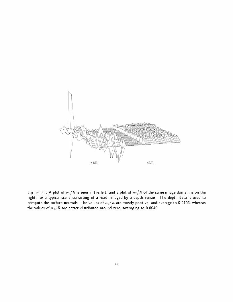
n1/R n2/R
Figure 6.1: A plot of n1=R is seen in the left, and a plot of n2=R of the same image domain is on the
right, for a typical scene consisting of a road, imaged by a depth sensor. The depth data is used to
compute the surface normals. The values of n2=R are mostly positive, and average to 0.0103, whereas
the values of n1=R are better distributed around zero, averaging to 0.0040.
56
More realistically, it is the average values of n1 and n2 throughout the image that in uences
the accuracy of the linear regression that is used to estimate the components of !. For example, if
n1 and n2 average to 0.1, then the previous bounds may be reduced by a factor of 10. Although
typical values of the average surface normal tilts must be determined empirically, many scenes
are composed of a variety of tilt directions. Such variety makes it possible to apply the surface
normal balancing technique. Fig. (6.1) shows plots of n1=R and n2=R for a typical scene of a road,
computed using depth data. The values of n1=R are well-distributed about zero, and average to
0.0040. The values of n2=R, on the other hand, are predominantly positive, and average to 0.0103.
The result is that using this scene, the value of the horizontal rotational component !1 is likely to
be estimated with greater error when using the ow circulation algorithm.
We observe in this example that the rotation component about the horizontal axis, !1, is
confounded by forward velocity and horizontal surfaces with large n2=R. Likewise, rotation about
the vertical axis, !2, which would arise as a sensor rotates from left to right, is confounded by a
forward velocity and a surface patch whose tilt lies horizontally.
Consider for instance a person walking next to a vertical wall (see Fig. (6.2)). Instantaneously,
the motion �eld induced by the wall can indicate either forward velocity or rotation of the head
away from the wall. As shown in Fig. (6.2), the two instantaneous ow �elds are similar, although
not equal. The curl of these ow �elds, along the wall, are equal (equal curls do not imply equal
vector �elds). In any given vertical slice along the wall, the ow �elds are qualitatively extremely
similar. The sense in which they di�er is that the magnitude of the vector �eld due to forward
translation decreases with the range, so that the velocity vectors are quite small at the far end of
the wall. Since the curls are identical, the ow circulation algorithm will not distinguish between
the two cases. The ambiguity may easily be resolved by higher-level processing, such as analyzing
over time the scene at the gaze point. A similar analysis shows that rotation about the line of
sight (optical axis) is readily confused with lateral motion with respect to a surface such that
�n2v1 + n1v2 is large.
Our conclusion is that for some scenes, the ow circulation algorithm should be able to estimate
the rotational parameters correctly; for other scenes, accurate estimation of rotational parameters
from the velocity �eld using the ow circulation algorithm is an unstable process, and that other
processing, such as scene analysis of the gaze point or global analysis of some feature of the ow
�eld in addition to the curl will be necessary.
The confounding of parameters is more general than what has been presented here. It has been
observed [35,2] that by reducing the size of the �eld of view, optical ows from a horizontal rotation
and that from a leftward FOE can be made to look very similar. We discuss this problem, with
an example, in the next section.
One interesting observation about this algorithm is that the most favorable case for the algo-
rithm in terms of depth structure, is the frontal planar situation. This should not be surprising
because in this algorithm, the quantities being computed are the rotational parameters whose
57
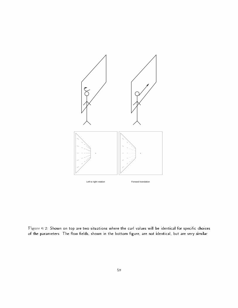
Left to right rotation
g
Forward translation
g
Figure 6.2: Shown on top are two situations where the curl values will be identical for speci�c choices
of the parameters. The ow �elds, shown in the bottom �gure, are not identical, but are very similar.
58
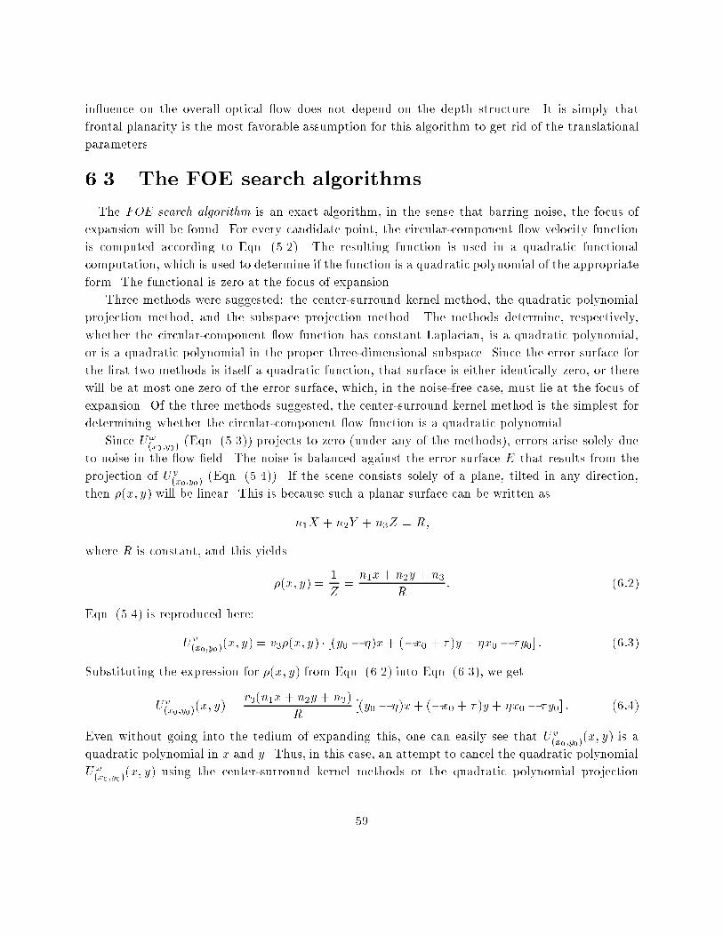
in uence on the overall optical ow does not depend on the depth structure. It is simply that
frontal planarity is the most favorable assumption for this algorithm to get rid of the translational
parameters.
6.3 The FOE search algorithms
The FOE search algorithm is an exact algorithm, in the sense that barring noise, the focus of
expansion will be found. For every candidate point, the circular-component ow velocity function
is computed according to Eqn. (5.2). The resulting function is used in a quadratic functional
computation, which is used to determine if the function is a quadratic polynomial of the appropriate
form. The functional is zero at the focus of expansion.
Three methods were suggested: the center-surround kernel method, the quadratic polynomial
projection method, and the subspace projection method. The methods determine, respectively,
whether the circular-component ow function has constant Laplacian, is a quadratic polynomial,
or is a quadratic polynomial in the proper three-dimensional subspace. Since the error surface for
the �rst two methods is itself a quadratic function, that surface is either identically zero, or there
will be at most one zero of the error surface, which, in the noise-free case, must lie at the focus of
expansion. Of the three methods suggested, the center-surround kernel method is the simplest for
determining whether the circular-component ow function is a quadratic polynomial.
Since U!(x0;y0)
(Eqn. (5.3)) projects to zero (under any of the methods), errors arise solely due
to noise in the ow �eld. The noise is balanced against the error surface E that results from the
projection of Uv(x0;y0)
(Eqn. (5.4)). If the scene consists solely of a plane, tilted in any direction,
then �(x; y) will be linear. This is because such a planar surface can be written as
n1X + n2Y + n3Z = R;
where R is constant, and this yields
�(x; y) =1
Z=
n1x+ n2y + n3R
: (6:2)
Eqn. (5.4) is reproduced here:
Uv(x0;y0)
(x; y) = v3�(x; y) � [(y0 � �)x+ (�x0 + �)y + �x0 � �y0] : (6:3)
Substituting the expression for �(x; y) from Eqn. (6.2) into Eqn. (6.3), we get
Uv(x0;y0)
(x; y) =v3(n1x+ n2y + n3)
R[(y0 � �)x+ (�x0 + �)y + �x0 � �y0] : (6:4)
Even without going into the tedium of expanding this, one can easily see that Uv(x0;y0)
(x; y) is a
quadratic polynomial in x and y. Thus, in this case, an attempt to cancel the quadratic polynomial
U!(x0;y0)
(x; y) using the center-surround kernel methods or the quadratic polynomial projection
59
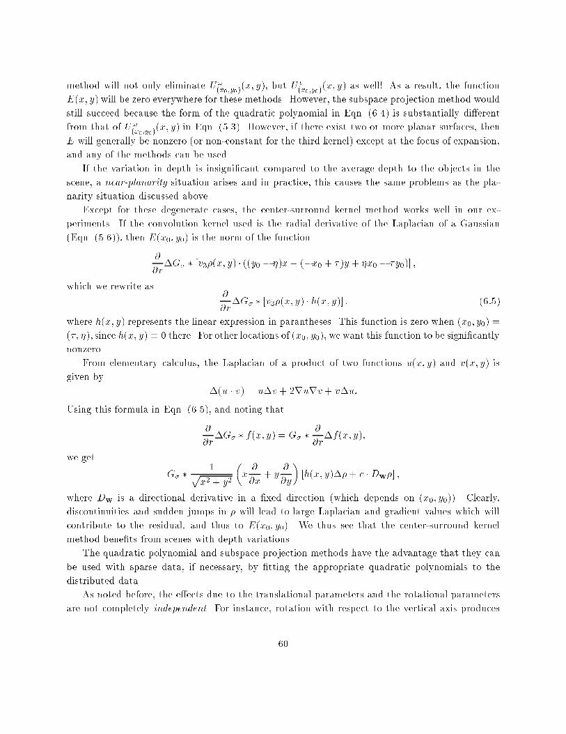
method will not only eliminate U!(x0;y0)
(x; y), but Uv(x0;y0)
(x; y) as well! As a result, the function
E(x; y) will be zero everywhere for these methods. However, the subspace projection method would
still succeed because the form of the quadratic polynomial in Eqn. (6.4) is substantially di�erent
from that of U!(x0;y0)
(x; y) in Eqn. (5.3). However, if there exist two or more planar surfaces, then
E will generally be nonzero (or non-constant for the third kernel) except at the focus of expansion,
and any of the methods can be used.
If the variation in depth is insigni�cant compared to the average depth to the objects in the
scene, a near-planarity situation arises and in practice, this causes the same problems as the pla-
narity situation discussed above.
Except for these degenerate cases, the center-surround kernel method works well in our ex-
periments. If the convolution kernel used is the radial derivative of the Laplacian of a Gaussian
(Eqn. (5.6)), then E(x0; y0) is the norm of the function
@
@r�G� � [v3�(x; y) � ((y0 � �)x+ (�x0 + �)y + �x0 � �y0)] ;
which we rewrite as@
@r�G� � [v3�(x; y) � h(x; y)] : (6:5)
where h(x; y) represents the linear expression in parantheses. This function is zero when (x0; y0) =
(�; �), since h(x; y) � 0 there. For other locations of (x0; y0), we want this function to be signi�cantly
nonzero.
From elementary calculus, the Laplacian of a product of two functions u(x; y) and v(x; y) is
given by
�(u � v) = u�v + 2rurv + v�u:
Using this formula in Eqn. (6.5), and noting that
@
@r�G� � f(x; y) = G� �
@
@r�f(x; y);
we get
G� �1p
x2 + y2
�x@
@x+ y
@
@y
�[h(x; y)��+ c �Dw�] ;
where Dw is a directional derivative in a �xed direction (which depends on (x0; y0)). Clearly,
discontinuities and sudden jumps in � will lead to large Laplacian and gradient values which will
contribute to the residual, and thus to E(x0; y0). We thus see that the center-surround kernel
method bene�ts from scenes with depth variations.
The quadratic polynomial and subspace projection methods have the advantage that they can
be used with sparse data, if necessary, by �tting the appropriate quadratic polynomials to the
distributed data.
As noted before, the e�ects due to the translational parameters and the rotational parameters
are not completely independent. For instance, rotation with respect to the vertical axis produces
60
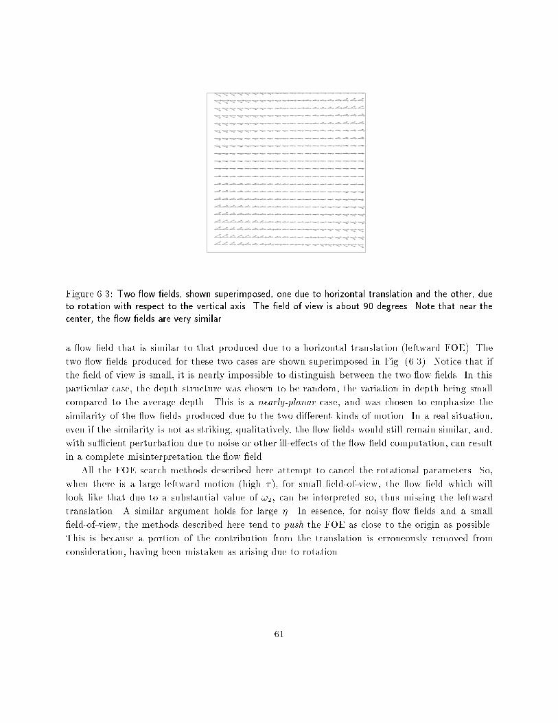
Figure 6.3: Two ow �elds, shown superimposed, one due to horizontal translation and the other, due
to rotation with respect to the vertical axis. The �eld of view is about 90 degrees. Note that near the
center, the ow �elds are very similar
a ow �eld that is similar to that produced due to a horizontal translation (leftward FOE). The
two ow �elds produced for these two cases are shown superimposed in Fig. (6.3). Notice that if
the �eld of view is small, it is nearly impossible to distinguish between the two ow �elds. In this
particular case, the depth structure was chosen to be random, the variation in depth being small
compared to the average depth. This is a nearly-planar case, and was chosen to emphasize the
similarity of the ow �elds produced due to the two di�erent kinds of motion. In a real situation,
even if the similarity is not as striking, qualitatively, the ow �elds would still remain similar, and,
with su�cient perturbation due to noise or other ill-e�ects of the ow �eld computation, can result
in a complete misinterpretation the ow �eld.
All the FOE search methods described here attempt to cancel the rotational parameters. So,
when there is a large leftward motion (high �), for small �eld-of-view, the ow �eld which will
look like that due to a substantial value of !2, can be interpreted so, thus missing the leftward
translation. A similar argument holds for large �. In essence, for noisy ow �elds and a small
�eld-of-view, the methods described here tend to push the FOE as close to the origin as possible.
This is because a portion of the contribution from the translation is erroneously removed from
consideration, having been mistaken as arising due to rotation.
61
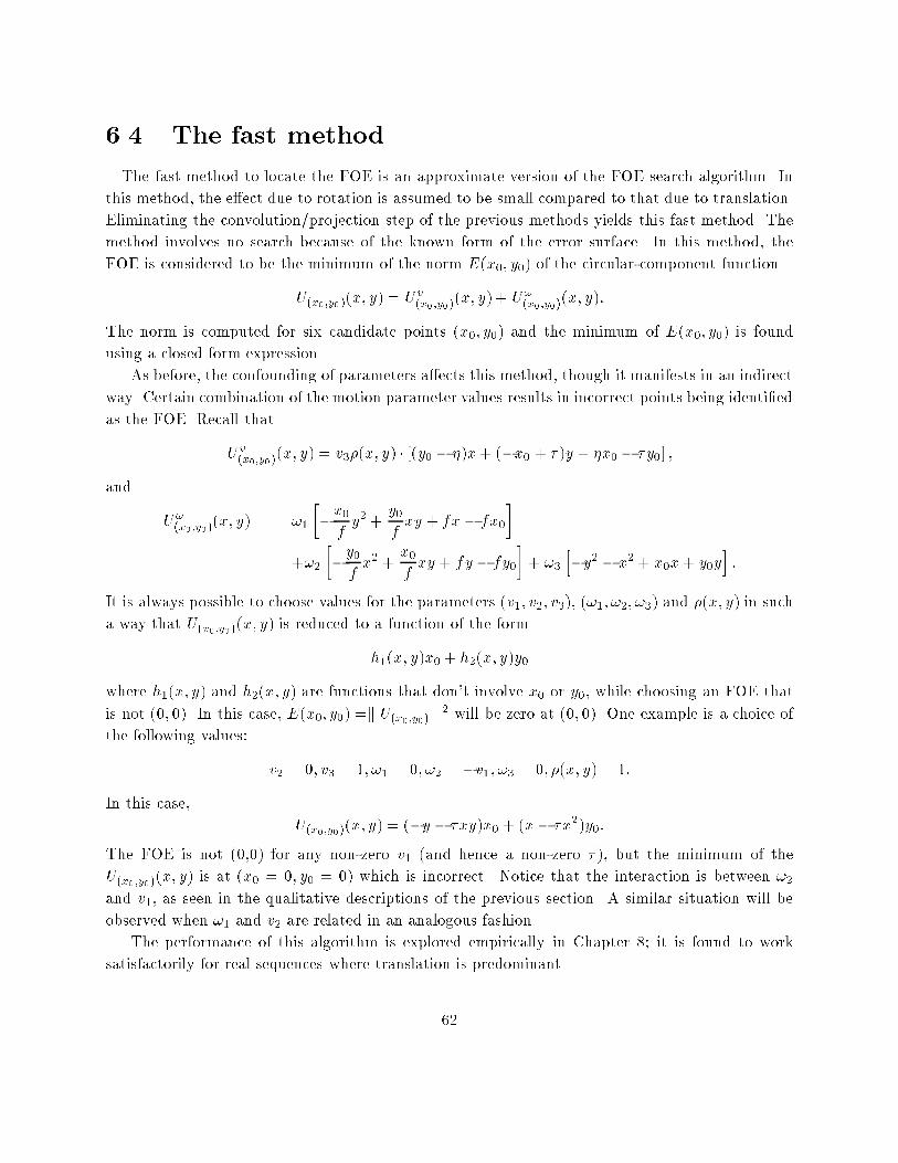
6.4 The fast method
The fast method to locate the FOE is an approximate version of the FOE search algorithm. In
this method, the e�ect due to rotation is assumed to be small compared to that due to translation.
Eliminating the convolution/projection step of the previous methods yields this fast method. The
method involves no search because of the known form of the error surface. In this method, the
FOE is considered to be the minimum of the norm E(x0; y0) of the circular-component function
U(x0;y0)(x; y) = Uv(x0;y0)
(x; y) + U!(x0;y0)
(x; y):
The norm is computed for six candidate points (x0; y0) and the minimum of E(x0; y0) is found
using a closed form expression.
As before, the confounding of parameters a�ects this method, though it manifests in an indirect
way. Certain combination of the motion parameter values results in incorrect points being identi�ed
as the FOE. Recall that
Uv(x0;y0)
(x; y) = v3�(x; y) � [(y0 � �)x+ (�x0 + �)y + �x0 � �y0] ;
and
U!(x0;y0)
(x; y) = !1
��x0fy2 +
y0fxy + fx � fx0
�
+!2
��y0fx2 +
x0fxy + fy � fy0
�+ !3
h�y2 � x2 + x0x+ y0y
i:
It is always possible to choose values for the parameters (v1; v2; v3), (!1; !2; !3) and �(x; y) in such
a way that U(x0;y0)(x; y) is reduced to a function of the form
h1(x; y)x0+ h2(x; y)y0
where h1(x; y) and h2(x; y) are functions that don't involve x0 or y0, while choosing an FOE that
is not (0; 0). In this case, E(x0; y0) =k U(x0;y0) k2 will be zero at (0; 0). One example is a choice of
the following values:
v2 = 0; v3 = 1; !1 = 0; !2 = �v1; !3 = 0; �(x; y) = 1:
In this case,
U(x0;y0)(x; y) = (�y � �xy)x0 + (x� �x2)y0:
The FOE is not (0,0) for any non-zero v1 (and hence a non-zero �), but the minimum of the
U(x0;y0)(x; y) is at (x0 = 0; y0 = 0) which is incorrect. Notice that the interaction is between !2and v1, as seen in the qualitative descriptions of the previous section. A similar situation will be
observed when !1 and v2 are related in an analogous fashion.
The performance of this algorithm is explored empirically in Chapter 8; it is found to work
satisfactorily for real sequences where translation is predominant.
62
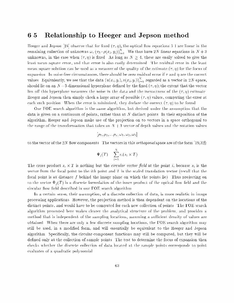
6.5 Relationship to Heeger and Jepson method
Heeger and Jepson [24] observe that for �xed (�; �), the optical ow equations 5.1 are linear in the
remaining collection of unknowns !, (v3 � �(xi; yi))Ni=1. We thus have 2N linear equations in N + 3
unknowns, in the case when (�; �) is �xed. As long as N � 4, these are easily solved to give the
least mean square error, and that error is also easily determined. The residual error in the least
mean square solution can be used as a measure of the quality of the estimate (�; �) for the focus of
expansion. In noise-free circumstances, there should be zero residual error if � and � are the correct
values. Equivalently, we see that the data (u(xi; yi); v(xi; yi))Ni=1 regarded as a vector in 2N -space,
should lie on an N+3-dimensional hyperplane de�ned by the �xed (�; �); the extent that the vector
lies o� this hyperplane measures the noise in the data and the inexactness of the (�; �) estimate.
Heeger and Jepson then simply check a large array of possible (�; �) values, computing the error at
each such position. When the error is minimized, they declare the correct (�; �) to be found.
Our FOE search algorithm is the same algorithm, but derived under the assumption that the
data is given on a continuum of points, rather than at N distinct points. In their exposition of the
algorithm, Heeger and Jepson make use of the projection on to vectors in a space orthogonal to
the range of the transformation that takes an N + 3 vector of depth values and the rotation values
[�1; �2; :::�n; !1; !2; !3]
to the vector of the 2N ow components. The vectors in this orthogonal space are of the form [19,32]:
j(T ) =NXi=1
ci(si � T )
The cross product si � T is nothing but the circular vector �eld at the point i, because si is the
vector from the focal point to the ith point and T is the scaled translation vector (recall that the
focal point is at distance f behind the image plane on which the points lie). Thus projecting on
to the vector j(T ) is a discrete formulation of the inner product of the optical ow �eld and the
circular ow �eld described in our FOE search algorithm.
In a certain sense, their assumption, of a discrete collection of data, is more realistic in image
processing applications. However, the projection method is then dependent on the locations of the
distinct points, and would have to be computed for each new collection of points. The FOE search
algorithm presented here makes clearer the analytical structure of the problem, and provides a
method that is independent of the sampling locations, assuming a su�cient density of values are
obtained. When there are only a few discrete sampling locations, the FOE search algorithm may
still be used, in a modi�ed form, and will essentially be equivalent to the Heeger and Jepson
algorithm. Speci�cally, the circular-component functions may still be computed, but they will be
de�ned only at the collection of sample points. The test to determine the focus of expansion then
checks whether the discrete collection of data located at the sample points corresponds to point
evaluates of a quadratic polynomial.
63

In the next two chapters, we will see the results of applying our algorithms to synthetic and
real data.
64
Chapter 7
Experimental Results: Synthetic
Data
7.1 Introduction
In the previous chapters, several methods to compute the motion parameters of a moving sensor
were presented and analyzed. In this chapter, we present the implementation details of the algo-
rithms and show experimental results from synthetic data. In the next chapter, we present results
from actual image sequences.
7.2 Rotation estimation
Recall that the rotation estimation method involves the computation of curl values at several
locations on the image plane. Three kinds of experiments are possible. The �rst is to determine
circulation values, which are equivalent to the curl values of the ow �eld at the centroids of the
circulation contour areas. The second way is to compute the curl values directly by taking discrete
di�erences; this is possible if the ow �eld is synthetic or not noisy. Alternatively, one can compute
the curl values analytically if the structure of the environment is known. Here we shall present
experiments of all these three types.
The optical ow �eld can be generated synthetically using the equations in (3.2), providing
the depth data (Z(x; y)) and the motion parameters (T and !) are known. If depth information
is available analytically or as the output of a sensor, we can synthesize ow �elds by choosing
appropriate values for the motion parameters. We begin by taking an object of known shape to be
in the environment and compute the curl values analytically.
Consider the image of an ellipsoid de�ned by
�X �X0
a
�2
+
�Y � Y0
b
�2
+
�Z � Z0
c
�2
= 1: (7:1)
65
We assume that the ellipsoid center is 150 focal units away (along the Z-axis), and the semiradii are
50, 30 and 70 focal units respectively. We assume the ellipsoid is in front of a planar background.
Choosing an observer moving with a velocity of (0:3; 0; 0:2) focal units per second, and rotating
with an angular velocity of (0:2; 0:1; 0:5) radians per second, we can analytically compute the
curl of the ow �eld. This is possible since we can compute @�@x
and @�@y, given the equation of the
ellipsoid in Eqn. (7.1). Recalling that � = 1=Z, x = fX=Z and y = fY=Z, multiplying both sides
of Eqn. (7.1) by f� and taking derivatives with respect to x, we get
@�
@x(x; y) =
1
d(x; y)
�x� f�X0
f2a2
�;
where d(x; y) is given by
d(x; y) =
��+
X0(x� f�X0)
fa2+Y0(y � f�Y0)
fb2+Z0(1� �Z0)
c2
�:
Note that the inverse depth is a function of x and y. For simplicity, we have written � instead of
�(x; y). Similarly, taking derivatives with respect to y, we get
@�
@y(x; y) =
1
d(x; y)
�y � f�X0
f2b2
�:
We can compute the curl values for any (x; y) which corresponds to the projection of a surface
point on the ellipsoid, using the computed gradient of � in the equation
r�V (x; y) =�@�
@x� (v3y � fv2)� @�
@y� (v3x� fv1)
�� 1
f[x!1 + y!2 + 2f!3] :
Knowing the geometry of the scene, for a given point (x; y), it is straightforward to determine if
the point is on the image of the ellipsoid or the background plane. Recall that for all the other
points (corresponding to a planar background), the translational part of the curl vanishes and only
the linear, rotational part remains.
The curl will have values as graphed in Fig. (7.1). The true linear surface is seen in the
background region (which is a frontal planar surface and hence gives the exact results); the distortion
in the other regions is caused by the translational velocity in conjunction with the surface tilts.
If there is an error in the determination of the curl of the vector �eld, then the resulting surface
shown in Fig. (7.1) will be perturbed. Estimates of the linear surface will most likely be based on
averaged values over regions, and not on local gradients of the displayed surface; the least squares
error estimate of the linear surface �nds the best-�tting plane. Clearly, the best-�t linear surface to
the surface shown in Fig. (7.1) will give an accurate estimate of the parameters of the unperturbed
linear surface. For the surface shown, the estimated rotation parameters are accurate to the fourth
decimal place. This example shows that accurate results can be obtained using the method, if there
is a good distribution of the surface normals about the normal to the frontal planar surface.
66
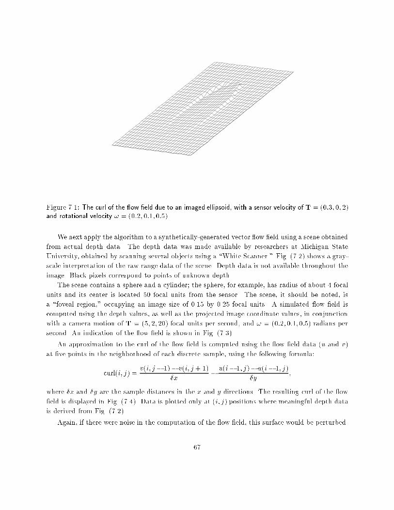
Figure 7.1: The curl of the ow �eld due to an imaged ellipsoid, with a sensor velocity of T = (0:3; 0; 2)and rotational velocity ! = (0:2; 0:1; 0:5).
We next apply the algorithm to a synthetically-generated vector ow �eld using a scene obtained
from actual depth data. The depth data was made available by researchers at Michigan State
University, obtained by scanning several objects using a \White Scanner." Fig. (7.2) shows a gray-
scale interpretation of the raw range data of the scene. Depth data is not available throughout the
image. Black pixels correspond to points of unknown depth.
The scene contains a sphere and a cylinder; the sphere, for example, has radius of about 4 focal
units and its center is located 50 focal units from the sensor. The scene, it should be noted, is
a \foveal region," occupying an image size of 0.15 by 0.25 focal units. A simulated ow �eld is
computed using the depth values, as well as the projected image coordinate values, in conjunction
with a camera motion of T = (5; 2; 20) focal units per second, and ! = (0:2; 0:1; 0:5) radians per
second. An indication of the ow �eld is shown in Fig. (7.3).
An approximation to the curl of the ow �eld is computed using the ow �eld data (u and v)
at �ve points in the neighborhood of each discrete sample, using the following formula:
curl(i; j) =v(i; j� 1)� v(i; j+ 1)
�x� u(i� 1; j)� u(i� 1; j)
�y;
where �x and �y are the sample distances in the x and y directions. The resulting curl of the ow
�eld is displayed in Fig. (7.4). Data is plotted only at (i; j) positions where meaningful depth data
is derived from Fig. (7.2).
Again, if there were noise in the computation of the ow �eld, this surface would be perturbed.
67
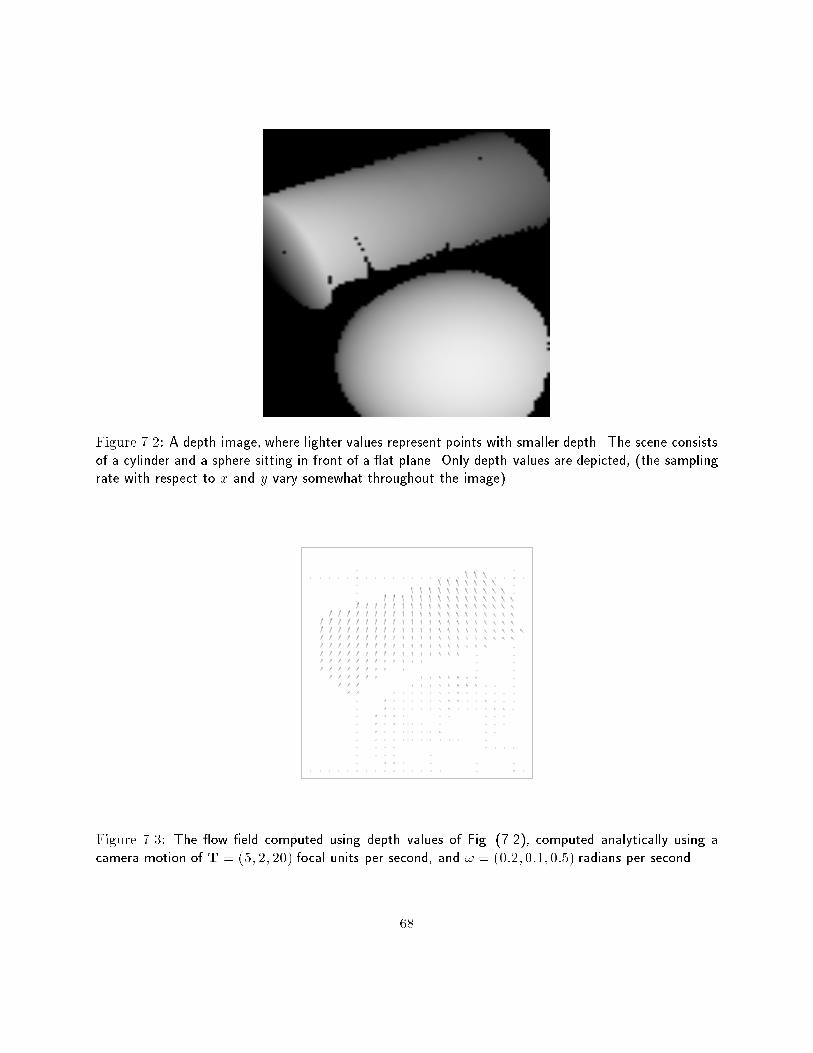
Figure 7.2: A depth image, where lighter values represent points with smaller depth. The scene consistsof a cylinder and a sphere sitting in front of a at plane. Only depth values are depicted, (the samplingrate with respect to x and y vary somewhat throughout the image).
Figure 7.3: The ow �eld computed using depth values of Fig. (7.2), computed analytically using acamera motion of T = (5; 2; 20) focal units per second, and ! = (0:2; 0:1; 0:5) radians per second.
68
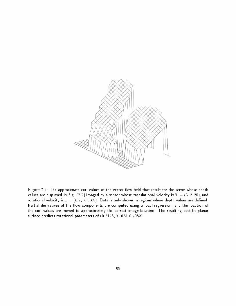
Figure 7.4: The approximate curl values of the vector ow �eld that result for the scene whose depthvalues are displayed in Fig. (7.2) imaged by a sensor whose translational velocity is T = (5; 2; 20), androtational velocity is ! = (0:2; 0:1; 0:5). Data is only shown in regions where depth values are de�ned.Partial derivatives of the ow components are computed using a local regression, and the location ofthe curl values are moved to approximately the correct image location. The resulting best-�t planarsurface predicts rotational parameters of (0:2126; 0:1023; 0:4982).
69
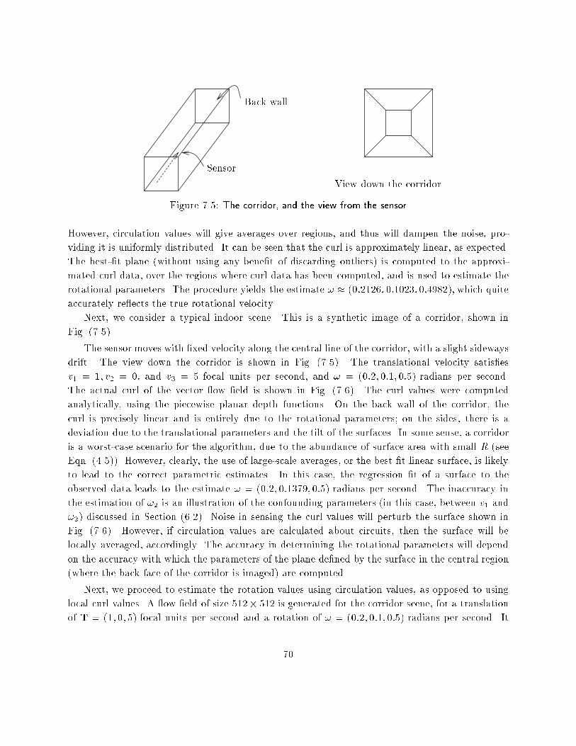
View down the corridor
Back wall
Sensor
Figure 7.5: The corridor, and the view from the sensor
However, circulation values will give averages over regions, and thus will dampen the noise, pro-
viding it is uniformly distributed. It can be seen that the curl is approximately linear, as expected.
The best-�t plane (without using any bene�t of discarding outliers) is computed to the approxi-
mated curl data, over the regions where curl data has been computed, and is used to estimate the
rotational parameters. The procedure yields the estimate ! � (0:2126; 0:1023; 0:4982), which quite
accurately re ects the true rotational velocity.
Next, we consider a typical indoor scene. This is a synthetic image of a corridor, shown in
Fig. (7.5).
The sensor moves with �xed velocity along the central line of the corridor, with a slight sideways
drift. The view down the corridor is shown in Fig. (7.5). The translational velocity satis�es
v1 = 1; v2 = 0, and v3 = 5 focal units per second, and ! = (0:2; 0:1; 0:5) radians per second.
The actual curl of the vector ow �eld is shown in Fig. (7.6). The curl values were computed
analytically, using the piecewise planar depth functions. On the back wall of the corridor, the
curl is precisely linear and is entirely due to the rotational parameters; on the sides, there is a
deviation due to the translational parameters and the tilt of the surfaces. In some sense, a corridor
is a worst-case scenario for the algorithm, due to the abundance of surface area with small R (see
Eqn. (4.5)). However, clearly, the use of large-scale averages, or the best �t linear surface, is likely
to lead to the correct parametric estimates. In this case, the regression �t of a surface to the
observed data leads to the estimate ! = (0:2; 0:1379; 0:5) radians per second. The inaccuracy in
the estimation of !2 is an illustration of the confounding parameters (in this case, between v1 and
!2) discussed in Section (6.2). Noise in sensing the curl values will perturb the surface shown in
Fig. (7.6). However, if circulation values are calculated about circuits, then the surface will be
locally averaged, accordingly. The accuracy in determining the rotational parameters will depend
on the accuracy with which the parameters of the plane de�ned by the surface in the central region
(where the back face of the corridor is imaged) are computed.
Next, we proceed to estimate the rotation values using circulation values, as opposed to using
local curl values. A ow �eld of size 512� 512 is generated for the corridor scene, for a translation
of T = (1; 0; 5) focal units per second and a rotation of ! = (0:2; 0:1; 0:5) radians per second. It
70
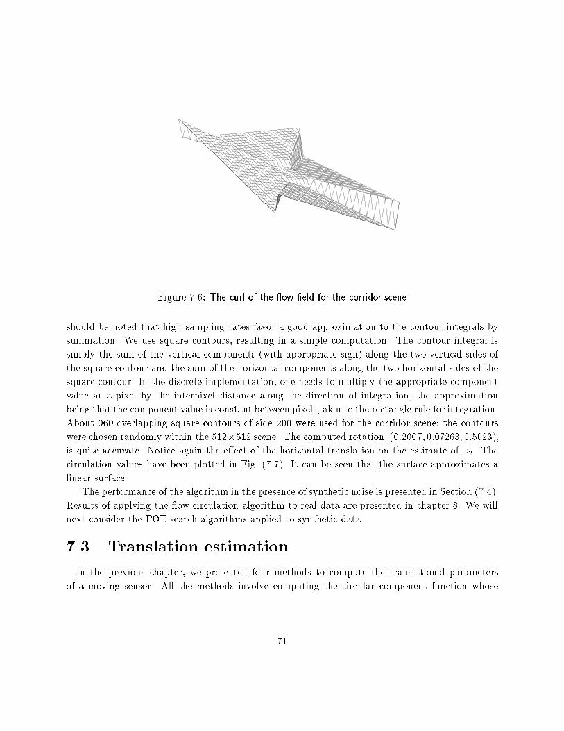
Figure 7.6: The curl of the ow �eld for the corridor scene
should be noted that high sampling rates favor a good approximation to the contour integrals by
summation. We use square contours, resulting in a simple computation. The contour integral is
simply the sum of the vertical components (with appropriate sign) along the two vertical sides of
the square contour and the sum of the horizontal components along the two horizontal sides of the
square contour. In the discrete implementation, one needs to multiply the appropriate component
value at a pixel by the interpixel distance along the direction of integration, the approximation
being that the component value is constant between pixels, akin to the rectangle rule for integration.
About 960 overlapping square contours of side 200 were used for the corridor scene; the contours
were chosen randomly within the 512�512 scene. The computed rotation, (0:2007; 0:07263; 0:5023),is quite accurate. Notice again the e�ect of the horizontal translation on the estimate of !2. The
circulation values have been plotted in Fig. (7.7). It can be seen that the surface approximates a
linear surface.
The performance of the algorithm in the presence of synthetic noise is presented in Section (7.4).
Results of applying the ow circulation algorithm to real data are presented in chapter 8. We will
next consider the FOE search algorithms applied to synthetic data.
7.3 Translation estimation
In the previous chapter, we presented four methods to compute the translational parameters
of a moving sensor. All the methods involve computing the circular component function whose
71
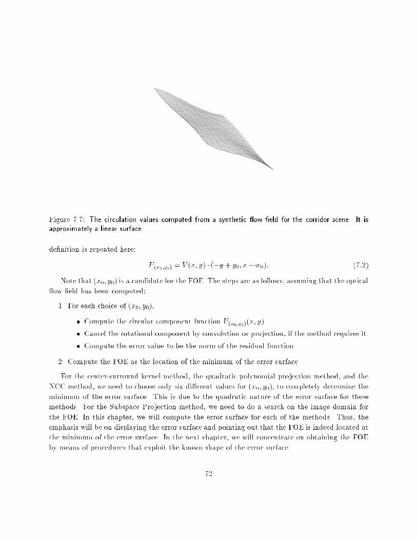
Figure 7.7: The circulation values computed from a synthetic ow �eld for the corridor scene. It isapproximately a linear surface.
de�nition is repeated here:
U(x0;y0) = V (x; y) � (�y + y0; x� x0): (7:2)
Note that (x0; y0) is a candidate for the FOE. The steps are as follows, assuming that the optical
ow �eld has been computed:
1. For each choice of (x0; y0),
� Compute the circular component function U(x0;y0)(x; y).
� Cancel the rotational component by convolution or projection, if the method requires it.
� Compute the error value to be the norm of the residual function.
2. Compute the FOE as the location of the minimum of the error surface.
For the center-surround kernel method, the quadratic polynomial projection method, and the
NCC method, we need to choose only six di�erent values for (x0; y0), to completely determine the
minimum of the error surface. This is due to the quadratic nature of the error surface for these
methods. For the Subspace Projection method, we need to do a search on the image domain for
the FOE. In this chapter, we will compute the error surface for each of the methods. Thus, the
emphasis will be on displaying the error surface and pointing out that the FOE is indeed located at
the minimum of the error surface. In the next chapter, we will concentrate on obtaining the FOE
by means of procedures that exploit the known shape of the error surface.
72
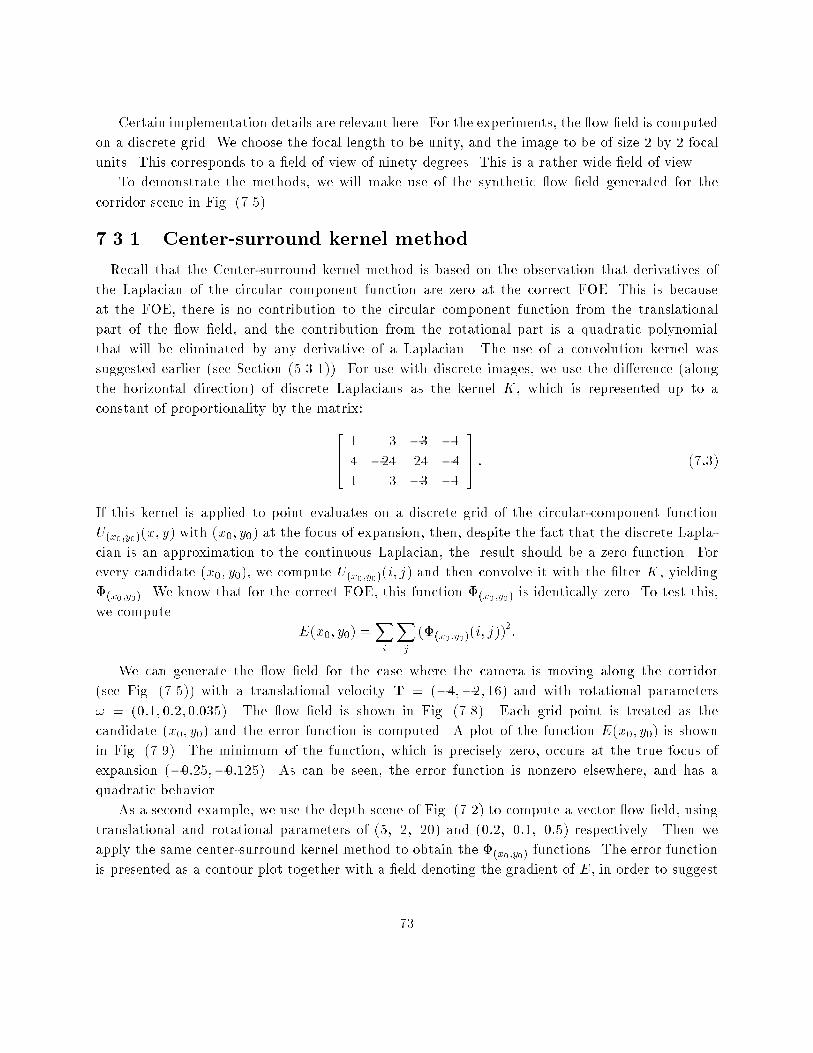
Certain implementation details are relevant here. For the experiments, the ow �eld is computed
on a discrete grid. We choose the focal length to be unity, and the image to be of size 2 by 2 focal
units. This corresponds to a �eld of view of ninety degrees. This is a rather wide �eld of view.
To demonstrate the methods, we will make use of the synthetic ow �eld generated for the
corridor scene in Fig. (7.5).
7.3.1 Center-surround kernel method
Recall that the Center-surround kernel method is based on the observation that derivatives of
the Laplacian of the circular component function are zero at the correct FOE. This is because
at the FOE, there is no contribution to the circular component function from the translational
part of the ow �eld, and the contribution from the rotational part is a quadratic polynomial
that will be eliminated by any derivative of a Laplacian. The use of a convolution kernel was
suggested earlier (see Section (5.3.1)). For use with discrete images, we use the di�erence (along
the horizontal direction) of discrete Laplacians as the kernel K, which is represented up to a
constant of proportionality by the matrix:
2641 3 �3 �14 �24 24 �41 3 �3 �1
375 : (7:3)
If this kernel is applied to point evaluates on a discrete grid of the circular-component function
U(x0;y0)(x; y) with (x0; y0) at the focus of expansion, then, despite the fact that the discrete Lapla-
cian is an approximation to the continuous Laplacian, the result should be a zero function. For
every candidate (x0; y0), we compute U(x0;y0)(i; j) and then convolve it with the �lter K, yielding
�(x0;y0). We know that for the correct FOE, this function �(x0;y0) is identically zero. To test this,
we compute
E(x0; y0) =Xi
Xj
(�(x0;y0)(i; j))2:
We can generate the ow �eld for the case where the camera is moving along the corridor
(see Fig. (7.5)) with a translational velocity T = (�4;�2; 16) and with rotational parameters
! = (0:1; 0:2; 0:035). The ow �eld is shown in Fig. (7.8). Each grid point is treated as the
candidate (x0; y0) and the error function is computed. A plot of the function E(x0; y0) is shown
in Fig. (7.9). The minimum of the function, which is precisely zero, occurs at the true focus of
expansion (�0:25;�0:125). As can be seen, the error function is nonzero elsewhere, and has a
quadratic behavior.
As a second example, we use the depth scene of Fig. (7.2) to compute a vector ow �eld, using
translational and rotational parameters of (5; 2; 20) and (0:2; 0:1; 0:5) respectively. Then we
apply the same center-surround kernel method to obtain the �(x0;y0) functions. The error function
is presented as a contour plot together with a �eld denoting the gradient of E, in order to suggest
73
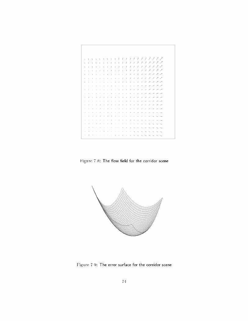
Figure 7.8: The ow �eld for the corridor scene
Figure 7.9: The error surface for the corridor scene
74
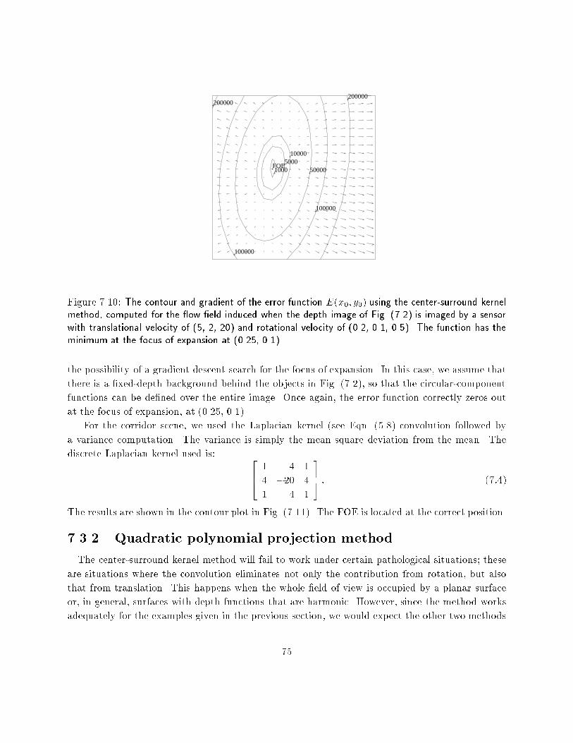
+FOE+1000
+5000+10000
+50000
+100000
+100000
+200000+200000
Figure 7.10: The contour and gradient of the error function E(x0; y0) using the center-surround kernelmethod, computed for the ow �eld induced when the depth image of Fig. (7.2) is imaged by a sensorwith translational velocity of (5, 2, 20) and rotational velocity of (0.2, 0.1, 0.5). The function has theminimum at the focus of expansion at (0.25, 0.1).
the possibility of a gradient descent search for the focus of expansion. In this case, we assume that
there is a �xed-depth background behind the objects in Fig. (7.2), so that the circular-component
functions can be de�ned over the entire image. Once again, the error function correctly zeros out
at the focus of expansion, at (0.25, 0.1).
For the corridor scene, we used the Laplacian kernel (see Eqn. (5.8) convolution followed by
a variance computation. The variance is simply the mean square deviation from the mean. The
discrete Laplacian kernel used is: 2641 4 1
4 �20 4
1 4 1
375 : (7:4)
The results are shown in the contour plot in Fig. (7.11). The FOE is located at the correct position.
7.3.2 Quadratic polynomial projection method
The center-surround kernel method will fail to work under certain pathological situations; these
are situations where the convolution eliminates not only the contribution from rotation, but also
that from translation. This happens when the whole �eld of view is occupied by a planar surface
or, in general, surfaces with depth functions that are harmonic. However, since the method works
adequately for the examples given in the previous section, we would expect the other two methods
75
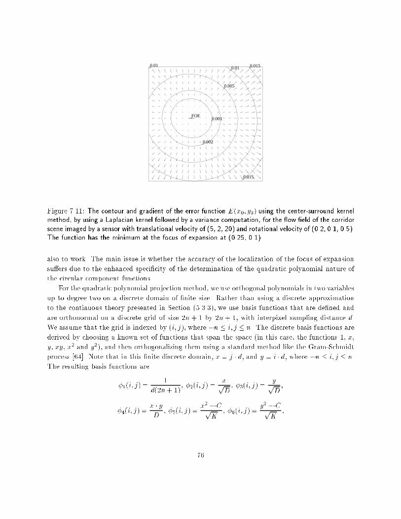
+FOE+0.001
+0.002
+0.005
+0.01+0.01
+0.015
+0.015
Figure 7.11: The contour and gradient of the error function E(x0; y0) using the center-surround kernelmethod, by using a Laplacian kernel followed by a variance computation, for the ow �eld of the corridorscene imaged by a sensor with translational velocity of (5, 2, 20) and rotational velocity of (0.2, 0.1, 0.5).The function has the minimum at the focus of expansion at (0.25, 0.1).
also to work. The main issue is whether the accuracy of the localization of the focus of expansion
su�ers due to the enhanced speci�city of the determination of the quadratic polynomial nature of
the circular component functions.
For the quadratic polynomial projection method, we use orthogonal polynomials in two variables
up to degree two on a discrete domain of �nite size. Rather than using a discrete approximation
to the continuous theory presented in Section (5.3.3), we use basis functions that are de�ned and
are orthonormal on a discrete grid of size 2n + 1 by 2n + 1, with interpixel sampling distance d.
We assume that the grid is indexed by (i; j), where �n � i; j � n. The discrete basis functions are
derived by choosing a known set of functions that span the space (in this case, the functions 1, x,
y, xy, x2 and y2), and then orthogonalizing them using a standard method like the Gram-Schmidt
process [64]. Note that in this �nite discrete domain, x = j � d, and y = i � d, where �n � i; j � n.
The resulting basis functions are
�1(i; j) =1
d(2n+ 1); �2(i; j) =
xpD; �3(i; j) =
ypD;
�4(i; j) =x � yD
; �5(i; j) =x2 � Cp
K; �6(i; j) =
y2 � CpK
;
76
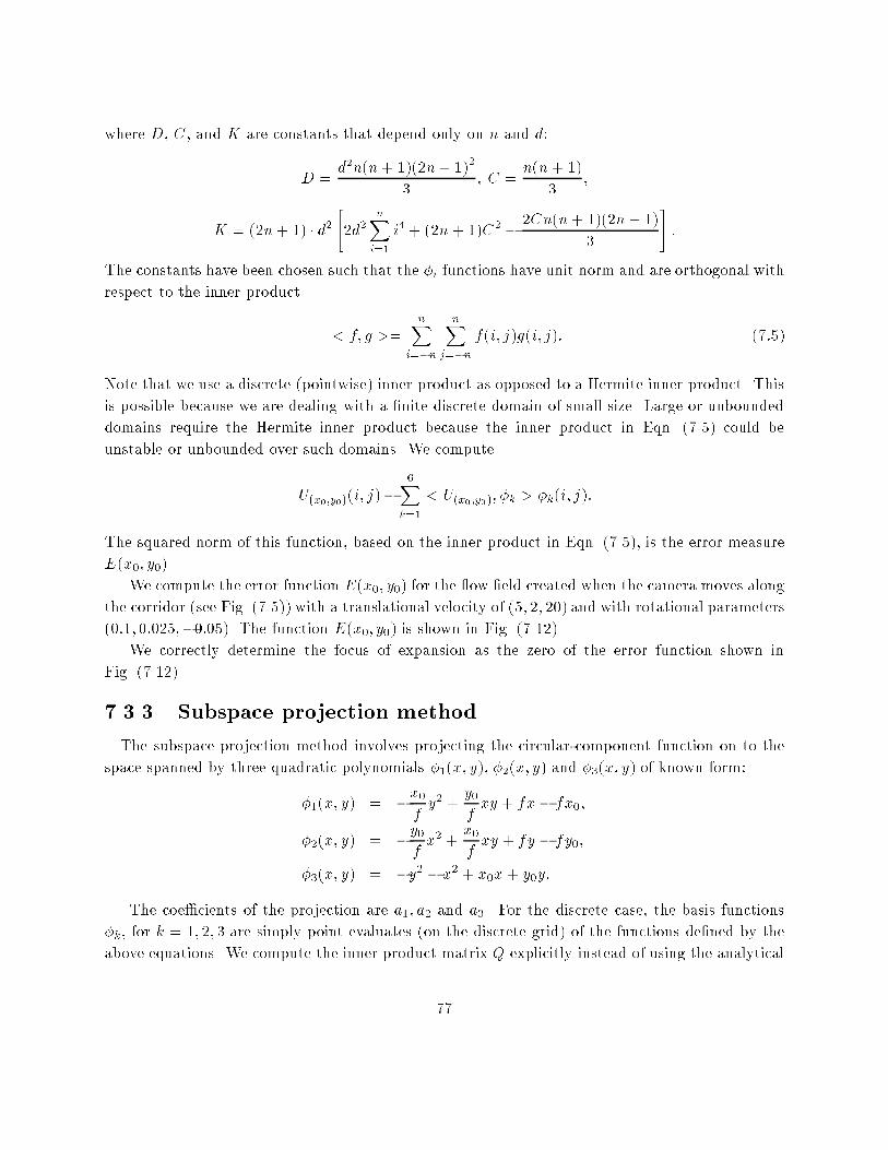
where D, C, and K are constants that depend only on n and d:
D =d2n(n+ 1)(2n+ 1)2
3; C =
n(n+ 1)
3;
K = (2n+ 1) � d2"2d2
nXi=1
i4 + (2n+ 1)C2 � 2Cn(n+ 1)(2n+ 1)
3
#:
The constants have been chosen such that the �i functions have unit norm and are orthogonal with
respect to the inner product
< f; g >=nX
i=�n
nXj=�n
f(i; j)g(i; j): (7:5)
Note that we use a discrete (pointwise) inner product as opposed to a Hermite inner product. This
is possible because we are dealing with a �nite discrete domain of small size. Large or unbounded
domains require the Hermite inner product because the inner product in Eqn. (7.5) could be
unstable or unbounded over such domains. We compute
U(x0;y0)(i; j)�6X
k=1
< U(x0;y0); �k > �k(i; j):
The squared norm of this function, based on the inner product in Eqn. (7.5), is the error measure
E(x0; y0).
We compute the error function E(x0; y0) for the ow �eld created when the camera moves along
the corridor (see Fig. (7.5)) with a translational velocity of (5; 2; 20) and with rotational parameters
(0:1; 0:025;�0:05). The function E(x0; y0) is shown in Fig. (7.12).
We correctly determine the focus of expansion as the zero of the error function shown in
Fig. (7.12).
7.3.3 Subspace projection method
The subspace projection method involves projecting the circular-component function on to the
space spanned by three quadratic polynomials �1(x; y), �2(x; y) and �3(x; y) of known form:
�1(x; y) = �x0fy2 +
y0fxy + fx� fx0;
�2(x; y) = �y0fx2 +
x0fxy + fy � fy0;
�3(x; y) = �y2 � x2 + x0x+ y0y:
The coe�cients of the projection are a1; a2 and a3. For the discrete case, the basis functions
�k, for k = 1; 2; 3 are simply point evaluates (on the discrete grid) of the functions de�ned by the
above equations. We compute the inner product matrix Q explicitly instead of using the analytical
77
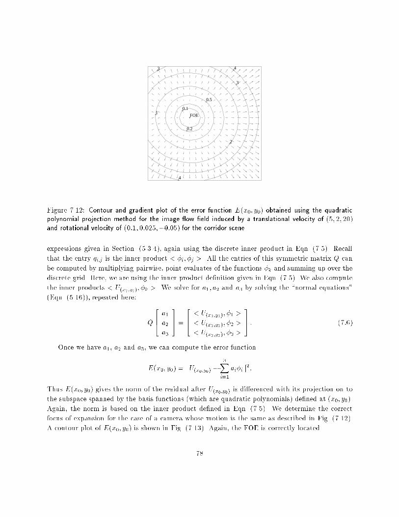
+FOE+0.1
+0.2
+0.5
+1
+2
+3
+3
+4
+4
Figure 7.12: Contour and gradient plot of the error function E(x0; y0) obtained using the quadraticpolynomial projection method for the image ow �eld induced by a translational velocity of (5; 2; 20)and rotational velocity of (0:1; 0:025;�0:05) for the corridor scene.
expressions given in Section. (5.3.4), again using the discrete inner product in Eqn. (7.5). Recall
that the entry qi;j is the inner product < �i; �j >. All the entries of this symmetric matrix Q can
be computed by multiplying pairwise, point evaluates of the functions �k and summing up over the
discrete grid. Here, we are using the inner product de�nition given in Eqn. (7.5). We also compute
the inner products < U(x0;y0); �k >. We solve for a1; a2 and a3 by solving the \normal equations"
(Eqn. (5.16)), repeated here:
Q
264a1a2a3
375 =
264< U(x0;y0); �1 >
< U(x0;y0); �2 >
< U(x0;y0); �3 >
375 : (7:6)
Once we have a1, a2 and a3, we can compute the error function
E(x0; y0) = kU(x0;y0) �3X
i=1
ai�ik2:
Thus E(x0; y0) gives the norm of the residual after U(x0;y0) is di�erenced with its projection on to
the subspace spanned by the basis functions (which are quadratic polynomials) de�ned at (x0; y0).
Again, the norm is based on the inner product de�ned in Eqn. (7.5). We determine the correct
focus of expansion for the case of a camera whose motion is the same as described in Fig. (7.12).
A contour plot of E(x0; y0) is shown in Fig. (7.13). Again, the FOE is correctly located.
78
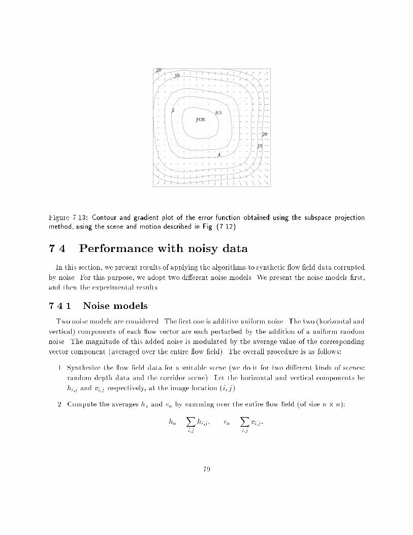
+FOE+0.5+2
+4
+10
+15
+20
+20
Figure 7.13: Contour and gradient plot of the error function obtained using the subspace projectionmethod, using the scene and motion described in Fig. (7.12).
7.4 Performance with noisy data
In this section, we present results of applying the algorithms to synthetic ow �eld data corrupted
by noise. For this purpose, we adopt two di�erent noise models. We present the noise models �rst,
and then the experimental results.
7.4.1 Noise models
Two noise models are considered. The �rst one is additive uniform noise. The two (horizontal and
vertical) components of each ow vector are each perturbed by the addition of a uniform random
noise. The magnitude of this added noise is modulated by the average value of the corresponding
vector component (averaged over the entire ow �eld). The overall procedure is as follows:
1. Synthesize the ow �eld data for a suitable scene (we do it for two di�erent kinds of scenes:
random depth data and the corridor scene). Let the horizontal and vertical components be
hi;j and vi;j respectively, at the image location (i; j).
2. Compute the averages ha and va by summing over the entire ow �eld (of size n � n):
ha =Xi;j
hi;j ; va =Xi;j
vi;j :
79
3. For each image location (i; j), perturb each component by a random value from a uniform
distribution, modulated by (a fraction of) the average values:
h0i;j = hi;j + f � ha � rhi;j; v0i;j = vi;j + f � va � rvi;j ;
where f is a fraction (a parameter in the experiments), and rh and rv are random values
distributed uniformly in the interval [�0:5; 0:5].
By varying the fraction f , the ow �eld is perturbed to varying extents and the algorithms
are tested on these ow �elds. For each value of f , each experiment is repeated several times (the
exact number is reported along with the results) and the error is averaged over the several runs.
The additive uniform noise model has been used before [24]. So, this method serves to compare
the results with previous ones.
The second model attempts to account for the way optical ow computations work. A majority
of the algorithms to compute optical ow use some form of regularization (smoothing), to overcome
the aperture problem. Because of this smoothing, the resulting optical ow, even though noisy,
tends to have noise components that are not independent identically distributed (i.i.d.), but are
correlated. To mimic this non-i.i.d. behavior, we add two di�erent noise components to the
synthetic ow �eld. First, we add Gaussian distributed random values to the magnitude of the
ow �eld vectors. Observation of error in real ow �elds suggests that Gaussian distribution is a
reasonable approximation [7,14]. Next, we add \smoothed" random values to the phase angle of the
ow �eld vectors, resulting in a systematic distortion of the ow �eld. Thus, the noise modulation
consists of two steps:
1. Let Mi;j and Pi;j be the magnitude and the phase angle of the (synthetic) optical ow vector
at image location (i; j). Add Gaussian random noise to the magnitude:
M 0
i;j =Mi;j � (1 + � � ri;j);
where ri;j is Gaussian randomly distributed with zero mean and unit variance (N(0; 1)), and
� is a fraction determining the extent of the noise modulation. Note that the additive noise
is proportional to the magnitude of individual ow vectors (as opposed to the average value
in the previous noise model).
2. Modulate the phase angles by a smoothed noise �eld:
P 0 = P + � � (r � s);
where r is randomly distributed noise with distribution N(0; 1), � is a fraction determining
the extent of the noise modulation, s is a smoothing �lter, and \�" indicates the convolutionoperation.
80
We generate synthetic ow �elds for both the corridor scene and random depth data. The
corridor scene is as described in Section 7.2. The random depth data is similar to the one used
in [24]; the depth values are randomly distributed uniformly between 2 units and 4 units, the unit
of measure being the focal length. The ow is computed over a grid of size 21�21. We next present
the results of applying the algorithms to the ow �elds with noise.
7.4.2 Experimental results with noisy data
We begin with experiments on the ow computed using random depth data. Depth values be-
tween 2 and 4 units were generated by sampling a uniform distribution. Recall (see Section 6.3)
that depth variations favor the FOE search algorithms. We synthesized ow �elds using a trans-
lation of v1 = 0:6, v2 = 0, and v3 = 0:8 units, and zero rotational velocity. The results are shown
in Fig. (7.14). The plots show the variation of the angular error (angle between the direction of
actual translation and the direction computed) with respect to the extent of noise, measured by
the fraction that modulates the noise amplitude.
For the uniform noise model, we note that the error is consistently the highest for the center-
surround kernel method, less for the quadratic polynomial projection method and the least for the
NCC algorithm. However, even for the value of f = 0:2, all the methods have errors below 2.5
degrees; this is quite accurate. For the smoothed Gaussian noise model, the worst performance is by
far the quadratic polynomial projection method, followed by the center-surround kernel method and
the NCC algorithm. Systematic distortions seem to be unfavorable for the quadratic polynomial
projection method. Also, all the methods have larger errors for this noise. Note that in both noise
situations, the NCC algorithm performs very well; it is to be expected, because there is no rotation,
and this is the best situation for the NCC algorithm.
In the second experiment, the parameters are the same as in the �rst, except that the rotation
is [0:0081;�0:0116;�0:0168] radians/sec (a typical angular velocity taken from an actual motion
sequence data). The results are shown in Fig. (7.15). As expected, the NCC algorithm has a
high error, even in the noise-free case (corresponding to f = 0 in the plots), but hardly degrades
with noise. The behavior of the other two methods is similar to that in the �rst experiment. In
both experiments, we see that the degradation with noise (for the noise models considered here) is
graceful. The error values are very low for the additive noise case, as in the zero angular velocity
situation. The errors are higher for the smoothed Gaussian noise, as before.
Next, we consider the corridor scene (Section 7.2). For the �rst experiment, we use a translation
of [5; 2; 20] units and zero angular velocity. The �eld of view is again about 30 degrees. The
error plots are in Fig. (7.16). The NCC algorithm has the best performance, and the quadratic
polynomial projection method has a performance comparable to the random depth data. However,
the center-surround kernel method has a much higher error rate, possibly due to the lack of large
depth variations.
Finally, we repeat the experiment for the case where the rotation is [0:0081� 0:0116� 0:0168].
81
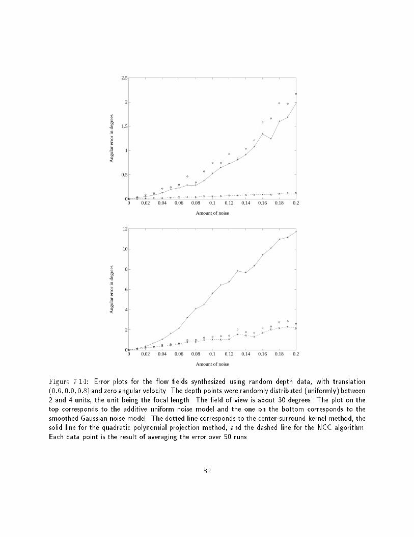
0
0.5
1
1.5
2
2.5
0 0.02 0.04 0.06 0.08 0.1 0.12 0.14 0.16 0.18 0.2
Amount of noise
Ang
ular
err
or in
deg
rees
o oo o
o oo
o
o
o
o o
oo
o
o
oo
o o
o
+ + + + ++ +
+ ++
+
++
+
+
+
+
+
++
+
x x x x x x x x x x x x x x x x x x x x x
0
2
4
6
8
10
12
0 0.02 0.04 0.06 0.08 0.1 0.12 0.14 0.16 0.18 0.2
Amount of noise
Ang
ular
err
or in
deg
rees
o o o o o o oo o
o o o o
oo o
o oo o
o
+ + ++
+
+
+
+
++
+
++
+ +
+
+
+
++
+
x x x x x x xx x x x x x
x x xx
x x x x
Figure 7.14: Error plots for the ow �elds synthesized using random depth data, with translation(0:6; 0:0; 0:8) and zero angular velocity. The depth points were randomly distributed (uniformly) between2 and 4 units, the unit being the focal length. The �eld of view is about 30 degrees. The plot on thetop corresponds to the additive uniform noise model and the one on the bottom corresponds to thesmoothed Gaussian noise model. The dotted line corresponds to the center-surround kernel method, thesolid line for the quadratic polynomial projection method, and the dashed line for the NCC algorithm.Each data point is the result of averaging the error over 50 runs.
82
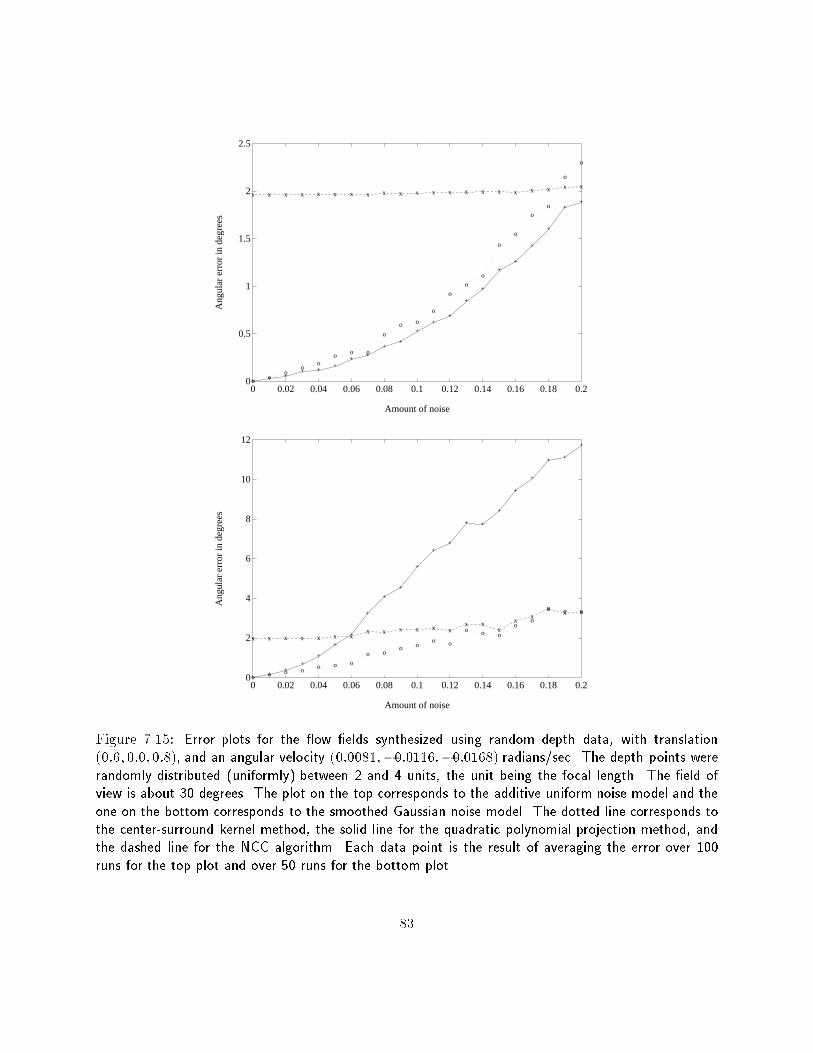
0
0.5
1
1.5
2
2.5
0 0.02 0.04 0.06 0.08 0.1 0.12 0.14 0.16 0.18 0.2
Amount of noise
Ang
ular
err
or in
deg
rees
o oo
oo
o o o
o
o o
o
oo
o
o
o
oo
o
o
+ + ++ +
++ +
++
++
+
+
+
++
+
+
++
x x x x x x x x x x x x x x x x x x x x x
0
2
4
6
8
10
12
0 0.02 0.04 0.06 0.08 0.1 0.12 0.14 0.16 0.18 0.2
Amount of noise
Ang
ular
err
or in
deg
rees
o o o o o o oo o
o oo o
o o o
oo
o o o
+ ++
++
+
+
+
++
+
++
+ +
+
+
+
+ +
+
x x x x x x xx x x x x x
x xx
xx
xx x
Figure 7.15: Error plots for the ow �elds synthesized using random depth data, with translation(0:6; 0:0; 0:8), and an angular velocity (0:0081;�0:0116;�0:0168) radians/sec. The depth points wererandomly distributed (uniformly) between 2 and 4 units, the unit being the focal length. The �eld ofview is about 30 degrees. The plot on the top corresponds to the additive uniform noise model and theone on the bottom corresponds to the smoothed Gaussian noise model. The dotted line corresponds tothe center-surround kernel method, the solid line for the quadratic polynomial projection method, andthe dashed line for the NCC algorithm. Each data point is the result of averaging the error over 100runs for the top plot and over 50 runs for the bottom plot.
83
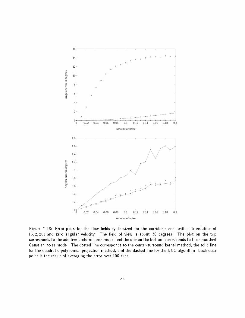
0
2
4
6
8
10
12
14
16
0 0.02 0.04 0.06 0.08 0.1 0.12 0.14 0.16 0.18 0.2
Amount of noise
Ang
ular
err
or in
deg
rees
o
o
o
o
o
o
o
o
oo
oo o o
o o o oo o o
+ + + + + + + + + + + + + + + + + + + + +
x x x x x x x x x x x x x x x x x x x x x
0
0.2
0.4
0.6
0.8
1
1.2
1.4
1.6
1.8
0 0.02 0.04 0.06 0.08 0.1 0.12 0.14 0.16 0.18 0.2
Amount of noise
Ang
ular
err
or in
deg
rees
o
o oo o
oo
oo o
o
o o oo
o o o
oo
o
+
+
+
+
+
+
+
++
++
+
+
++
+
+
++
+
+
xx
xx x
x xx
xx
xx
xx
x
x x x x x
x
Figure 7.16: Error plots for the ow �elds synthesized for the corridor scene, with a translation of(5; 2; 20) and zero angular velocity. The �eld of view is about 30 degrees. The plot on the topcorresponds to the additive uniform noise model and the one on the bottom corresponds to the smoothedGaussian noise model. The dotted line corresponds to the center-surround kernel method, the solid linefor the quadratic polynomial projection method, and the dashed line for the NCC algorithm. Each datapoint is the result of averaging the error over 100 runs.
84
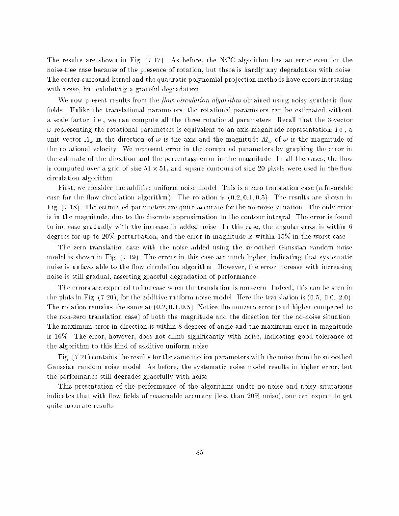
The results are shown in Fig. (7.17). As before, the NCC algorithm has an error even for the
noise-free case because of the presence of rotation, but there is hardly any degradation with noise.
The center-surround kernel and the quadratic polynomial projection methods have errors increasing
with noise, but exhibiting a graceful degradation.
We now present results from the ow circulation algorithm obtained using noisy synthetic ow
�elds. Unlike the translational parameters, the rotational parameters can be estimated without
a scale factor; i.e., we can compute all the three rotational parameters. Recall that the 3-vector
! representing the rotational parameters is equivalent to an axis-magnitude representation; i.e., a
unit vector A! in the direction of ! is the axis and the magnitude M! of ! is the magnitude of
the rotational velocity. We represent error in the computed parameters by graphing the error in
the estimate of the direction and the percentage error in the magnitude. In all the cases, the ow
is computed over a grid of size 51� 51, and square contours of side 20 pixels were used in the ow
circulation algorithm.
First, we consider the additive uniform noise model. This is a zero translation case (a favorable
case for the ow circulation algorithm). The rotation is (0:2; 0:1; 0:5). The results are shown in
Fig. (7.18). The estimated parameters are quite accurate for the no-noise situation. The only error
is in the magnitude, due to the discrete approximation to the contour integral. The error is found
to increase gradually with the increase in added noise. In this case, the angular error is within 6
degrees for up to 20% perturbation, and the error in magnitude is within 15% in the worst case.
The zero translation case with the noise added using the smoothed Gaussian random noise
model is shown in Fig. (7.19). The errors in this case are much higher, indicating that systematic
noise is unfavorable to the ow circulation algorithm. However, the error increase with increasing
noise is still gradual, asserting graceful degradation of performance.
The errors are expected to increase when the translation is non-zero. Indeed, this can be seen in
the plots in Fig. (7.20), for the additive uniform noise model. Here the translation is (0:5; 0:0; 2:0).
The rotation remains the same at (0:2; 0:1; 0:5). Notice the nonzero error (and higher compared to
the non-zero translation case) of both the magnitude and the direction for the no-noise situation.
The maximum error in direction is within 8 degrees of angle and the maximum error in magnitude
is 16%. The error, however, does not climb signi�cantly with noise, indicating good tolerance of
the algorithm to this kind of additive uniform noise.
Fig. (7.21) contains the results for the same motion parameters with the noise from the smoothed
Gaussian random noise model. As before, the systematic noise model results in higher error, but
the performance still degrades gracefully with noise.
This presentation of the performance of the algorithms under no-noise and noisy situtations
indicates that with ow �elds of reasonable accuracy (less than 20% noise), one can expect to get
quite accurate results.
85
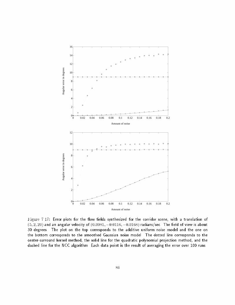
0
2
4
6
8
10
12
14
16
0 0.02 0.04 0.06 0.08 0.1 0.12 0.14 0.16 0.18 0.2
Amount of noise
Ang
ular
err
or in
deg
rees
o
o
o
o
o
o
o
o
oo
oo
o oo o o o
o o o
+ + + + + + + + + + + + + + + + + + + + +
x x x x x x x x x x x x x x x x x x x x x
0
2
4
6
8
10
12
0 0.02 0.04 0.06 0.08 0.1 0.12 0.14 0.16 0.18 0.2
Amount of noise
Ang
ular
err
or in
deg
rees
o
o
o
o
oo
o oo o o o o o o o o o o o o
+ + + ++
++
++
++
++
++
++
++
+ +
x x x x x x x x x x x x x x x x x x x x x
Figure 7.17: Error plots for the ow �elds synthesized for the corridor scene, with a translation of(5; 2; 20) and an angular velocity of (0:0081;�0:0116;�0:0168) radians/sec. The �eld of view is about30 degrees. The plot on the top corresponds to the additive uniform noise model and the one onthe bottom corresponds to the smoothed Gaussian noise model. The dotted line corresponds to thecenter-surround kernel method, the solid line for the quadratic polynomial projection method, and thedashed line for the NCC algorithm. Each data point is the result of averaging the error over 100 runs.
86
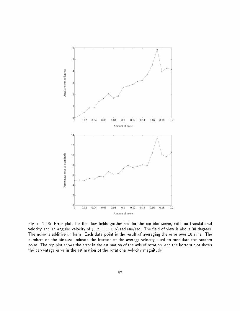
0
1
2
3
4
5
6
0 0.02 0.04 0.06 0.08 0.1 0.12 0.14 0.16 0.18 0.2o
o
o
o o
oo
o
oo
oo
o
o o
o
o
o
o
o o
Ang
ular
err
or in
deg
rees
Amount of noise
0
2
4
6
8
10
12
14
0 0.02 0.04 0.06 0.08 0.1 0.12 0.14 0.16 0.18 0.2
o o oo o
o o
oo o
o
oo
oo o
o
o
oo
o
Perc
enta
ge e
rror
of
mag
nitu
de
Amount of noise
Figure 7.18: Error plots for the ow �elds synthesized for the corridor scene, with no translationalvelocity and an angular velocity of (0:2; 0:1; 0:5) radians/sec. The �eld of view is about 30 degrees.The noise is additive uniform. Each data point is the result of averaging the error over 10 runs. Thenumbers on the abscissa indicate the fraction of the average velocity, used to modulate the randomnoise. The top plot shows the error in the estimation of the axis of rotation, and the bottom plot showsthe percentage error in the estimation of the rotational velocity magnitude.
87
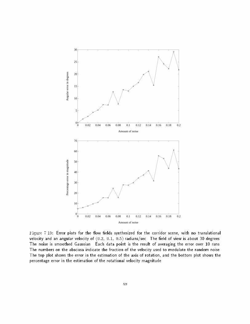
0
5
10
15
20
25
30
0 0.02 0.04 0.06 0.08 0.1 0.12 0.14 0.16 0.18 0.2o
oo
oo
o o
o
o
oo
o
o
o
o
o
o
o
o
o
oA
ngul
ar e
rror
in d
egre
es
Amount of noise
0
10
20
30
40
50
60
70
0 0.02 0.04 0.06 0.08 0.1 0.12 0.14 0.16 0.18 0.2
oo
oo
o
o o
o
o
o oo
o
o
o
o
oo
o
o
o
Perc
enta
ge e
rror
in m
agni
tude
Amount of noise
Figure 7.19: Error plots for the ow �elds synthesized for the corridor scene, with no translationalvelocity and an angular velocity of (0:2; 0:1; 0:5) radians/sec. The �eld of view is about 30 degrees.The noise is smoothed Gaussian. Each data point is the result of averaging the error over 10 runs.The numbers on the abscissa indicate the fraction of the velocity used to modulate the random noise.The top plot shows the error in the estimation of the axis of rotation, and the bottom plot shows thepercentage error in the estimation of the rotational velocity magnitude.
88
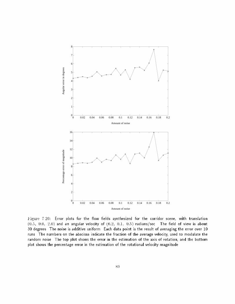
0
1
2
3
4
5
6
7
8
0 0.02 0.04 0.06 0.08 0.1 0.12 0.14 0.16 0.18 0.2
o o oo
o
o
oo o
o
o
o
o
o o
o
o
o
o
oo
Amount of noise
Ang
ular
err
or in
deg
rees
0
2
4
6
8
10
12
14
16
0 0.02 0.04 0.06 0.08 0.1 0.12 0.14 0.16 0.18 0.2
o o o o o
o
o
oo
o
o
o
o
o o
o
o
o
o
oo
Perc
enta
ge e
rror
of
mag
nitu
de
Amount of noise
Figure 7.20: Error plots for the ow �elds synthesized for the corridor scene, with translation(0:5; 0:0; 2:0) and an angular velocity of (0:2; 0:1; 0:5) radians/sec. The �eld of view is about30 degrees. The noise is additive uniform. Each data point is the result of averaging the error over 10runs. The numbers on the abscissa indicate the fraction of the average velocity, used to modulate therandom noise. The top plot shows the error in the estimation of the axis of rotation, and the bottomplot shows the percentage error in the estimation of the rotational velocity magnitude.
89
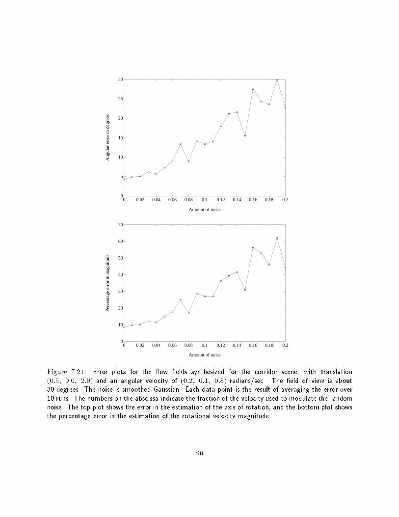
0
5
10
15
20
25
30
0 0.02 0.04 0.06 0.08 0.1 0.12 0.14 0.16 0.18 0.2
oo o
o o
o
o
o
o
oo
o
o
o o
o
o
oo
o
oA
ngul
ar e
rror
in d
egre
es
Amount of noise
0
10
20
30
40
50
60
70
0 0.02 0.04 0.06 0.08 0.1 0.12 0.14 0.16 0.18 0.2
oo o
o o
o
o
o
o
oo o
o
oo
o
o
o
o
o
o
Amount of noise
Perc
enta
ge e
rror
in m
agni
tude
Figure 7.21: Error plots for the ow �elds synthesized for the corridor scene, with translation(0:5; 0:0; 2:0) and an angular velocity of (0:2; 0:1; 0:5) radians/sec. The �eld of view is about30 degrees. The noise is smoothed Gaussian. Each data point is the result of averaging the error over10 runs. The numbers on the abscissa indicate the fraction of the velocity used to modulate the randomnoise. The top plot shows the error in the estimation of the axis of rotation, and the bottom plot showsthe percentage error in the estimation of the rotational velocity magnitude.
90
Chapter 8
Experimental Results: Real Data
8.1 Introduction
In this chapter, we present the results from applying the algorithms to real image sequences.
Two di�erent methods were used to compute the ow �elds. One is the multiscale matching
approach of Anandan [5], and the other is a multiscale MRF procedure [25]. Brief descriptions of
the multiscale matching method of Anandan and the multiscale MRF procedure were presented in
Section 2.4 of Chapter 2.
In most of the experiments, we compare the computed motion parameters to the parameters
available from the calibration information. The structure computation is possible only for relatively
noise-free ow �elds because relative depth is local information encoded in the optical ow vectors
in a pointwise fashion. So, in some of the experiments, we compute the relative depth (structure)
information and display the computed depth data much like a range map.
The implementation details are identical to those described in the previous chapter about ex-
periments on synthetic data, unless otherwise noted.
8.2 The Straight ight sequence
This sequence was shot from a helicopter ying in a straight line, with very little rotational
velocity. A sample picture from the sequence is shown in Fig. 8.1. The ow �eld was computed
using the multiscale matching method. The original images are of the size 512 � 512 pixels. The
ow �elds were computed at a lower resolution (128� 128) to save computation time and space.
The results of the Center-surround kernel method (with the horizontal di�erential of a Lapla-
cian, as in Eqn. (5.7)) are shown in Fig. (8.2). The FOEs computed using the variance of the
output of the convolution with a Laplacian kernel (Eqn. (5.8)) are shown in Fig. (8.3). The results
of the quadratic polynomial projection method, computed using the same ow �elds, are shown
in Fig. (8.4). The results of using the subspace projection method and the fast (approximate)
method are in Fig. (8.5) and Fig. (8.6) respectively. Angular measurements of errors are shown in
91
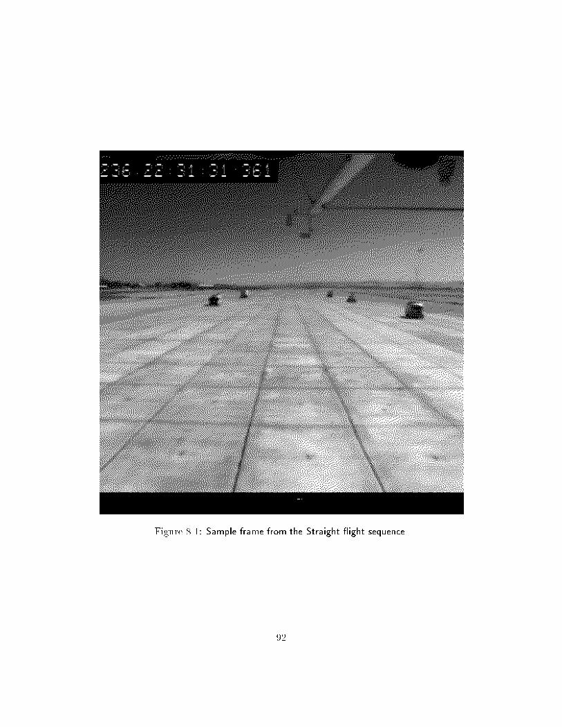
Figure 8.1: Sample frame from the Straight ight sequence.
92
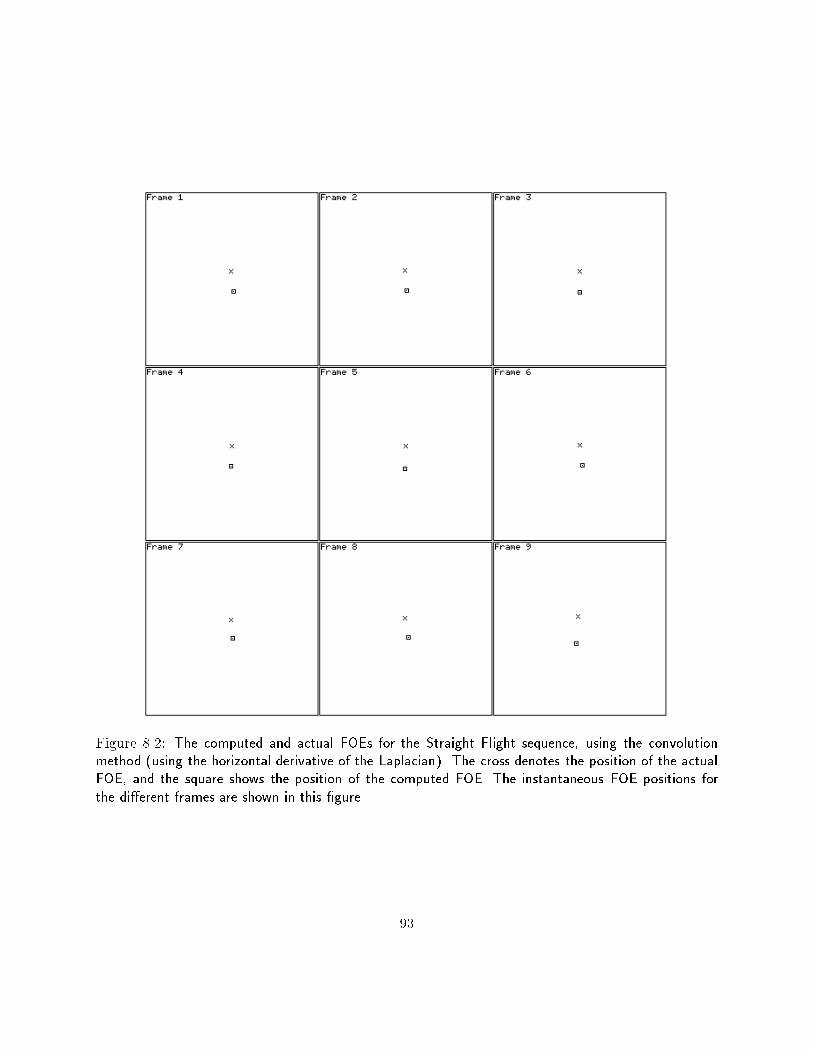
Figure 8.2: The computed and actual FOEs for the Straight Flight sequence, using the convolutionmethod (using the horizontal derivative of the Laplacian). The cross denotes the position of the actualFOE, and the square shows the position of the computed FOE. The instantaneous FOE positions forthe di�erent frames are shown in this �gure.
93
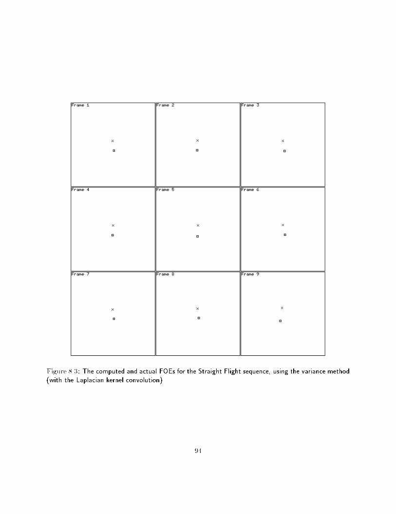
Figure 8.3: The computed and actual FOEs for the Straight Flight sequence, using the variance method(with the Laplacian kernel convolution).
94
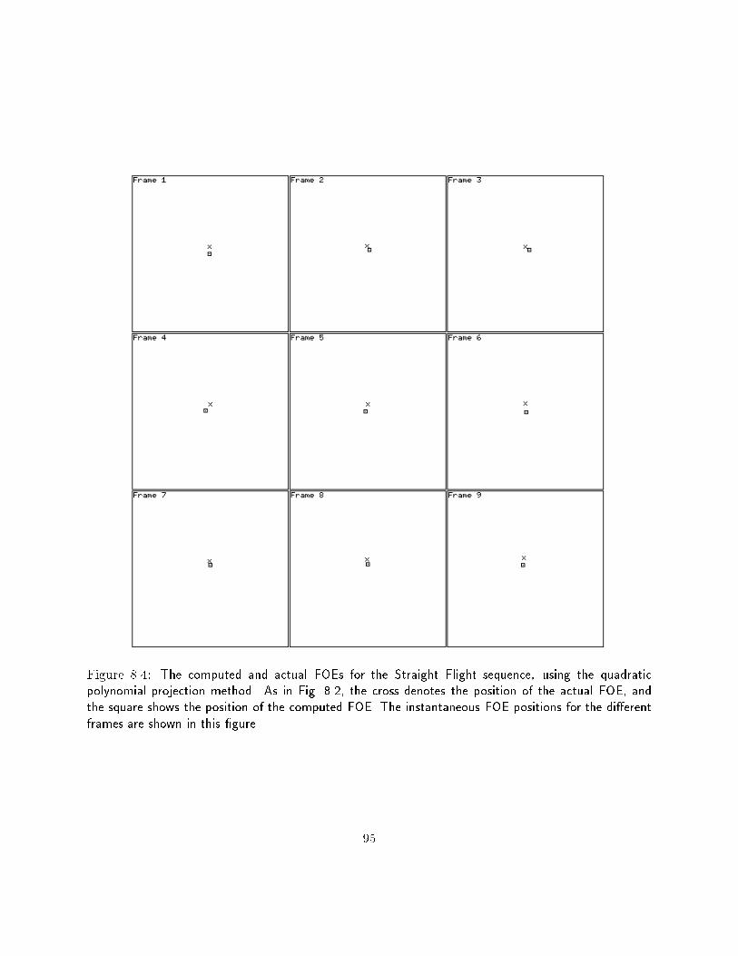
Figure 8.4: The computed and actual FOEs for the Straight Flight sequence, using the quadraticpolynomial projection method. As in Fig. 8.2, the cross denotes the position of the actual FOE, andthe square shows the position of the computed FOE. The instantaneous FOE positions for the di�erentframes are shown in this �gure.
95
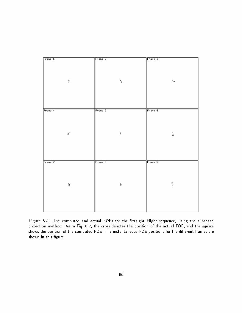
Figure 8.5: The computed and actual FOEs for the Straight Flight sequence, using the subspaceprojection method. As in Fig. 8.2, the cross denotes the position of the actual FOE, and the squareshows the position of the computed FOE. The instantaneous FOE positions for the di�erent frames areshown in this �gure.
96
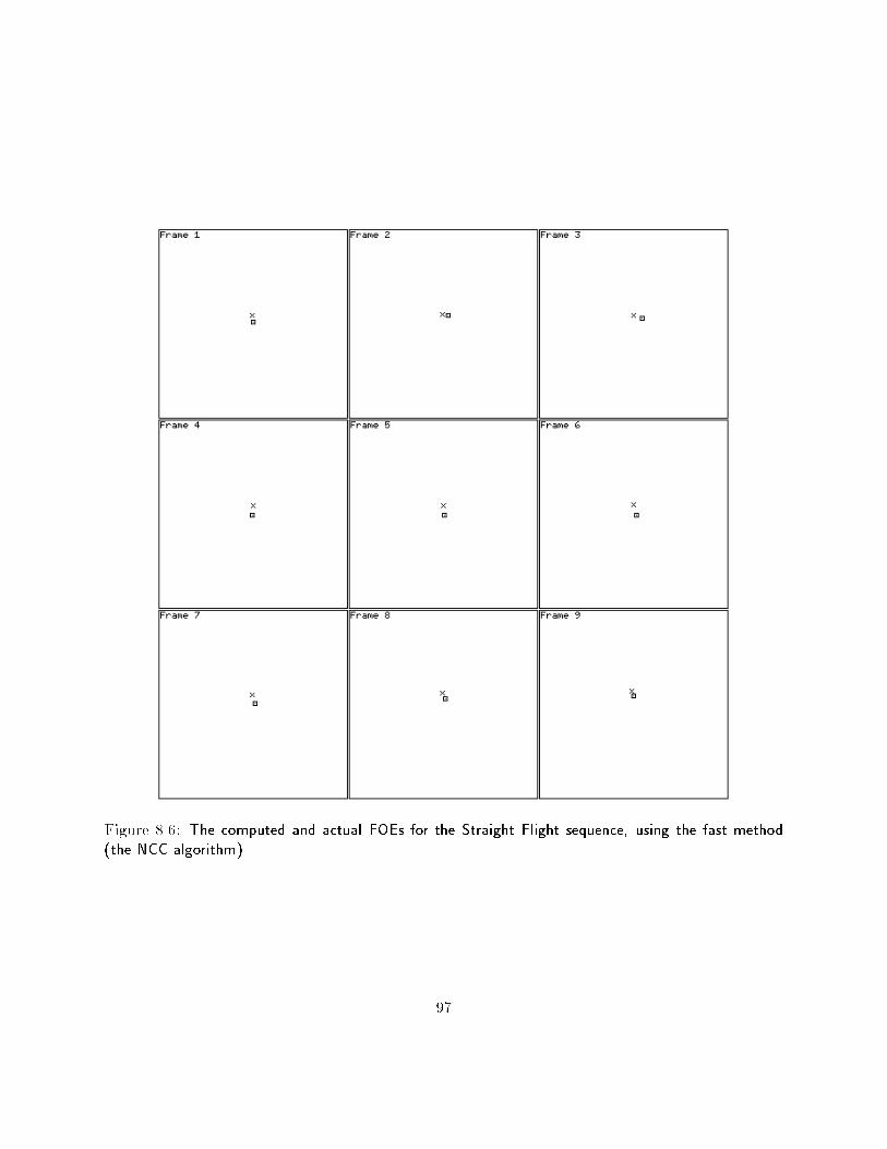
Figure 8.6: The computed and actual FOEs for the Straight Flight sequence, using the fast method(the NCC algorithm).
97
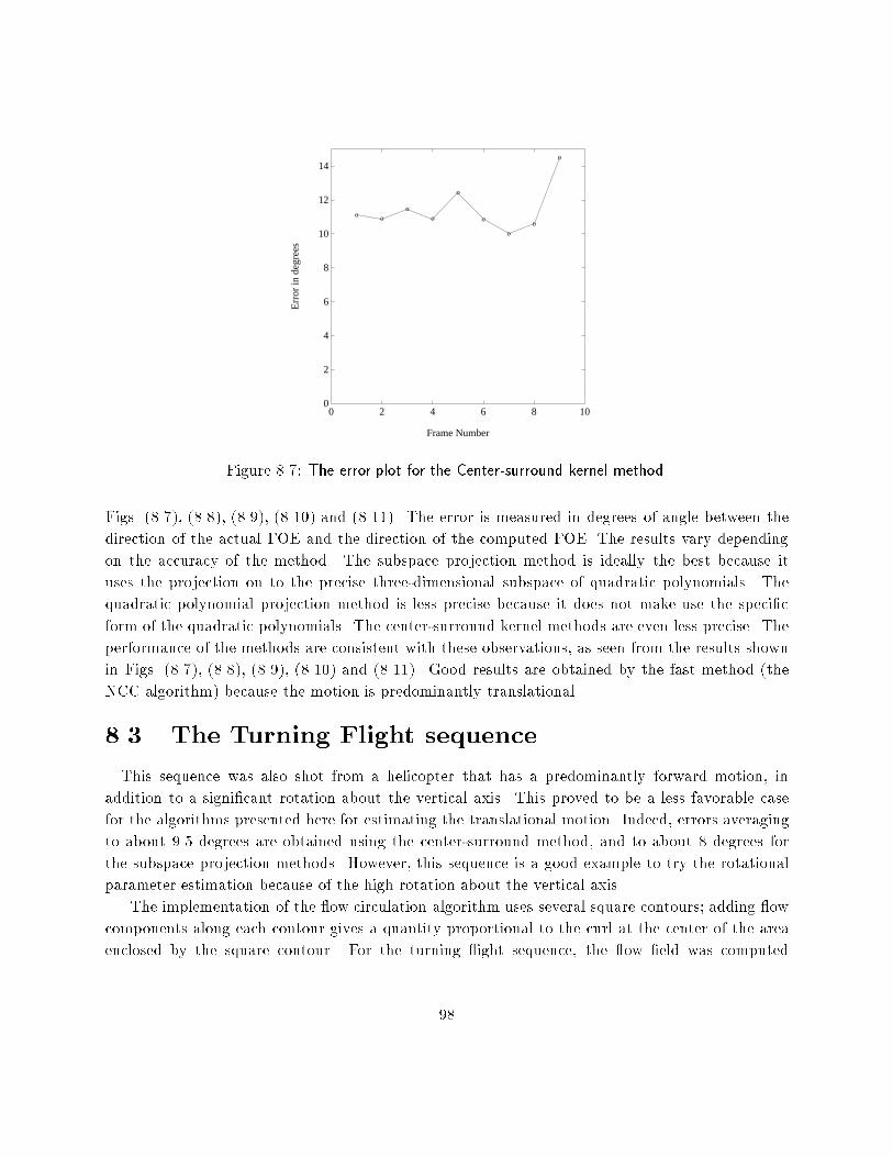
0
2
4
6
8
10
12
14
0 2 4 6 8 10
o oo
o
o
o
oo
o
Frame Number
Err
or in
deg
rees
Figure 8.7: The error plot for the Center-surround kernel method.
Figs. (8.7), (8.8), (8.9), (8.10) and (8.11). The error is measured in degrees of angle between the
direction of the actual FOE and the direction of the computed FOE. The results vary depending
on the accuracy of the method. The subspace projection method is ideally the best because it
uses the projection on to the precise three-dimensional subspace of quadratic polynomials. The
quadratic polynomial projection method is less precise because it does not make use the speci�c
form of the quadratic polynomials. The center-surround kernel methods are even less precise. The
performance of the methods are consistent with these observations, as seen from the results shown
in Figs. (8.7), (8.8), (8.9), (8.10) and (8.11). Good results are obtained by the fast method (the
NCC algorithm) because the motion is predominantly translational.
8.3 The Turning Flight sequence
This sequence was also shot from a helicopter that has a predominantly forward motion, in
addition to a signi�cant rotation about the vertical axis. This proved to be a less favorable case
for the algorithms presented here for estimating the translational motion. Indeed, errors averaging
to about 9.5 degrees are obtained using the center-surround method, and to about 8 degrees for
the subspace projection methods. However, this sequence is a good example to try the rotational
parameter estimation because of the high rotation about the vertical axis.
The implementation of the ow circulation algorithm uses several square contours; adding ow
components along each contour gives a quantity proportional to the curl at the center of the area
enclosed by the square contour. For the turning ight sequence, the ow �eld was computed
98
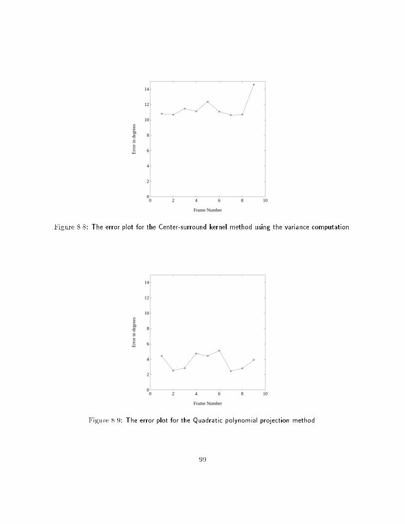
0
2
4
6
8
10
12
14
0 2 4 6 8 10
o o
oo
o
oo o
o
Err
or in
deg
rees
Frame Number
Figure 8.8: The error plot for the Center-surround kernel method using the variance computation.
0
2
4
6
8
10
12
14
0 2 4 6 8 10
o
oo
oo
o
oo
o
Frame Number
Err
or in
deg
rees
Figure 8.9: The error plot for the Quadratic polynomial projection method.
99
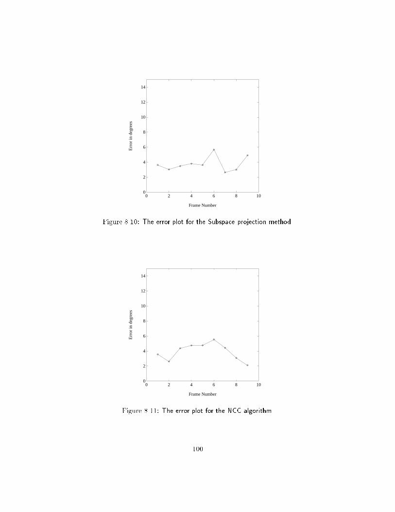
0
2
4
6
8
10
12
14
0 2 4 6 8 10
o
oo
o o
o
oo
o
Frame Number
Err
or in
deg
rees
Figure 8.10: The error plot for the Subspace projection method.
0
2
4
6
8
10
12
14
0 2 4 6 8 10
o
o
oo o
o
o
o
o
Frame Number
Err
or in
deg
rees
Figure 8.11: The error plot for the NCC algorithm.
100
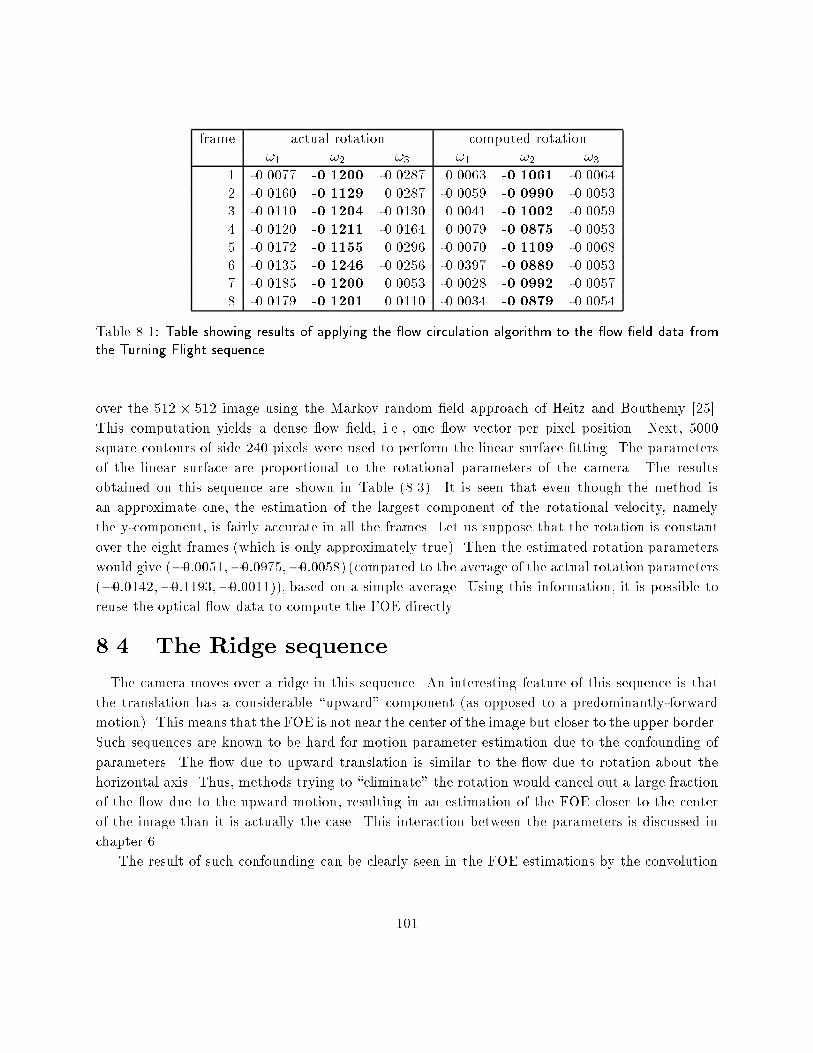
frame actual rotation computed rotation!1 !2 !3 !1 !2 !3
1 -0.0077 -0.1200 -0.0287 0.0063 -0.1061 -0.00642 -0.0160 -0.1129 0.0287 -0.0059 -0.0990 -0.00533 -0.0110 -0.1204 -0.0130 0.0041 -0.1002 -0.00594 -0.0120 -0.1211 -0.0164 0.0079 -0.0875 -0.00535 -0.0172 -0.1155 0.0296 -0.0070 -0.1109 -0.00686 -0.0135 -0.1246 -0.0256 -0.0397 -0.0889 -0.00537 -0.0185 -0.1200 0.0053 -0.0028 -0.0992 -0.00578 -0.0179 -0.1201 0.0110 -0.0034 -0.0879 -0.0054
Table 8.1: Table showing results of applying the ow circulation algorithm to the ow �eld data fromthe Turning Flight sequence.
over the 512 � 512 image using the Markov random �eld approach of Heitz and Bouthemy [25].
This computation yields a dense ow �eld, i.e., one ow vector per pixel position. Next, 5000
square contours of side 240 pixels were used to perform the linear surface �tting. The parameters
of the linear surface are proportional to the rotational parameters of the camera. The results
obtained on this sequence are shown in Table (8.3). It is seen that even though the method is
an approximate one, the estimation of the largest component of the rotational velocity, namely
the y-component, is fairly accurate in all the frames. Let us suppose that the rotation is constant
over the eight frames (which is only approximately true). Then the estimated rotation parameters
would give (�0:0051;�0:0975;�0:0058) (compared to the average of the actual rotation parameters
(�0:0142;�0:1193;�0:0011)), based on a simple average. Using this information, it is possible to
reuse the optical ow data to compute the FOE directly.
8.4 The Ridge sequence
The camera moves over a ridge in this sequence. An interesting feature of this sequence is that
the translation has a considerable \upward" component (as opposed to a predominantly-forward
motion). This means that the FOE is not near the center of the image but closer to the upper border.
Such sequences are known to be hard for motion parameter estimation due to the confounding of
parameters. The ow due to upward translation is similar to the ow due to rotation about the
horizontal axis. Thus, methods trying to \eliminate" the rotation would cancel out a large fraction
of the ow due to the upward motion, resulting in an estimation of the FOE closer to the center
of the image than it is actually the case. This interaction between the parameters is discussed in
chapter 6.
The result of such confounding can be clearly seen in the FOE estimations by the convolution
101
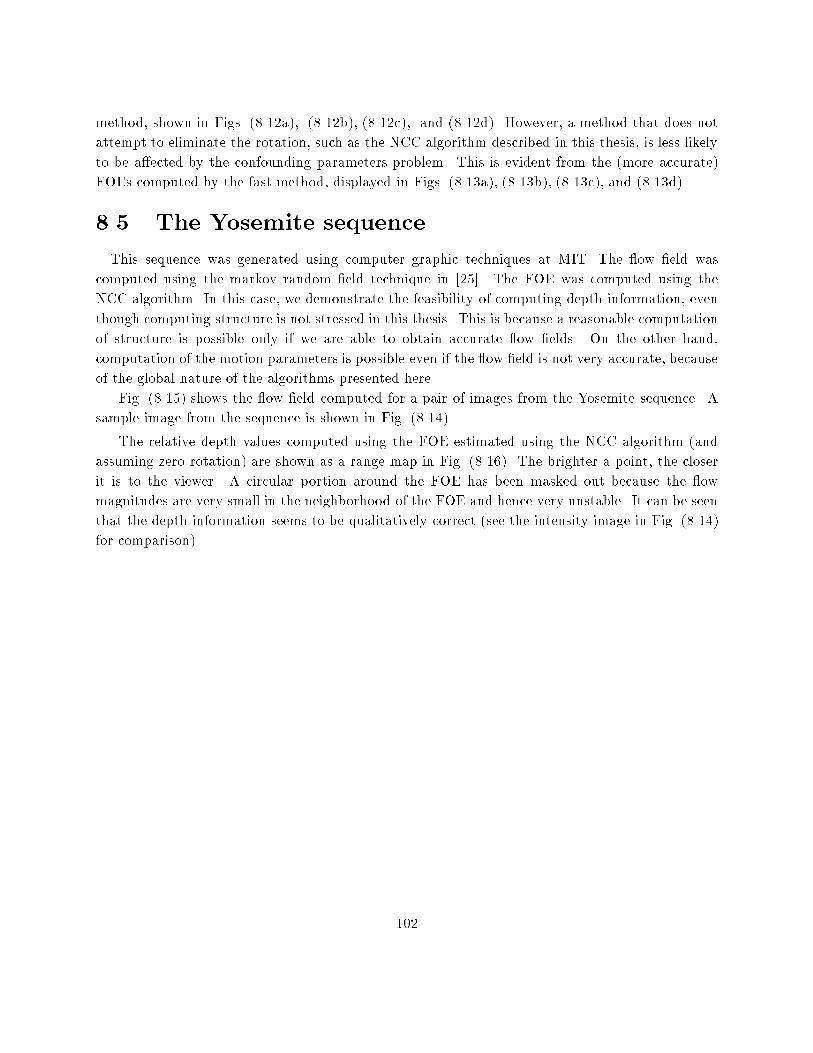
method, shown in Figs. (8.12a), (8.12b), (8.12c), and (8.12d). However, a method that does not
attempt to eliminate the rotation, such as the NCC algorithm described in this thesis, is less likely
to be a�ected by the confounding parameters problem. This is evident from the (more accurate)
FOEs computed by the fast method, displayed in Figs. (8.13a), (8.13b), (8.13c), and (8.13d).
8.5 The Yosemite sequence
This sequence was generated using computer graphic techniques at MIT. The ow �eld was
computed using the markov random �eld technique in [25]. The FOE was computed using the
NCC algorithm. In this case, we demonstrate the feasibility of computing depth information, even
though computing structure is not stressed in this thesis. This is because a reasonable computation
of structure is possible only if we are able to obtain accurate ow �elds. On the other hand,
computation of the motion parameters is possible even if the ow �eld is not very accurate, because
of the global nature of the algorithms presented here.
Fig. (8.15) shows the ow �eld computed for a pair of images from the Yosemite sequence. A
sample image from the sequence is shown in Fig. (8.14).
The relative depth values computed using the FOE estimated using the NCC algorithm (and
assuming zero rotation) are shown as a range map in Fig. (8.16). The brighter a point, the closer
it is to the viewer. A circular portion around the FOE has been masked out because the ow
magnitudes are very small in the neighborhood of the FOE and hence very unstable. It can be seen
that the depth information seems to be qualitatively correct (see the intensity image in Fig. (8.14)
for comparison).
102
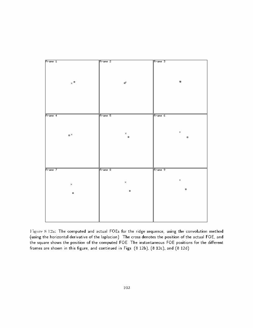
Figure 8.12a: The computed and actual FOEs for the ridge sequence, using the convolution method(using the horizontal derivative of the laplacian). The cross denotes the position of the actual FOE, andthe square shows the position of the computed FOE. The instantaneous FOE positions for the di�erentframes are shown in this �gure, and continued in Figs. (8.12b), (8.12c), and (8.12d).
103

Figure 8.12b: See the note in Fig. (8.12a).
104
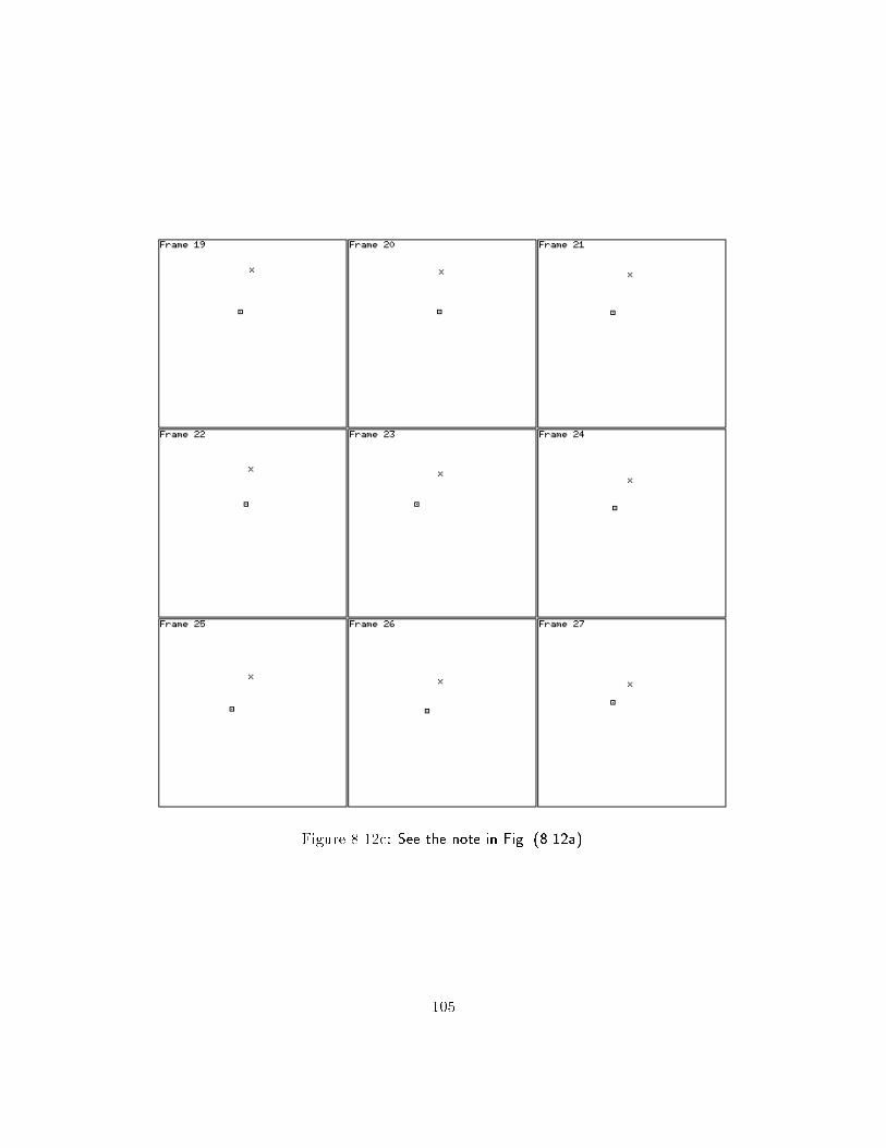
Figure 8.12c: See the note in Fig. (8.12a).
105
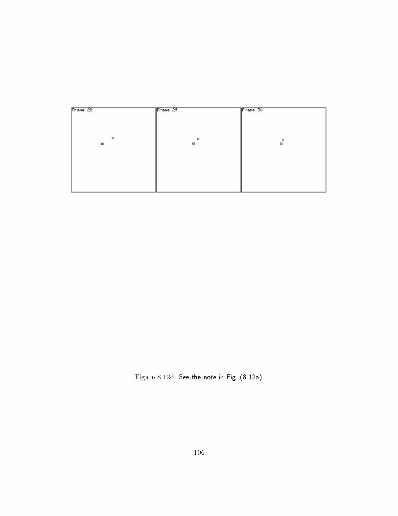
Figure 8.12d: See the note in Fig. (8.12a).
106
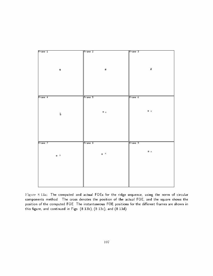
Figure 8.13a: The computed and actual FOEs for the ridge sequence, using the norm of circularcomponents method. The cross denotes the position of the actual FOE, and the square shows theposition of the computed FOE. The instantaneous FOE positions for the di�erent frames are shown inthis �gure, and continued in Figs. (8.13b), (8.13c), and (8.13d).
107
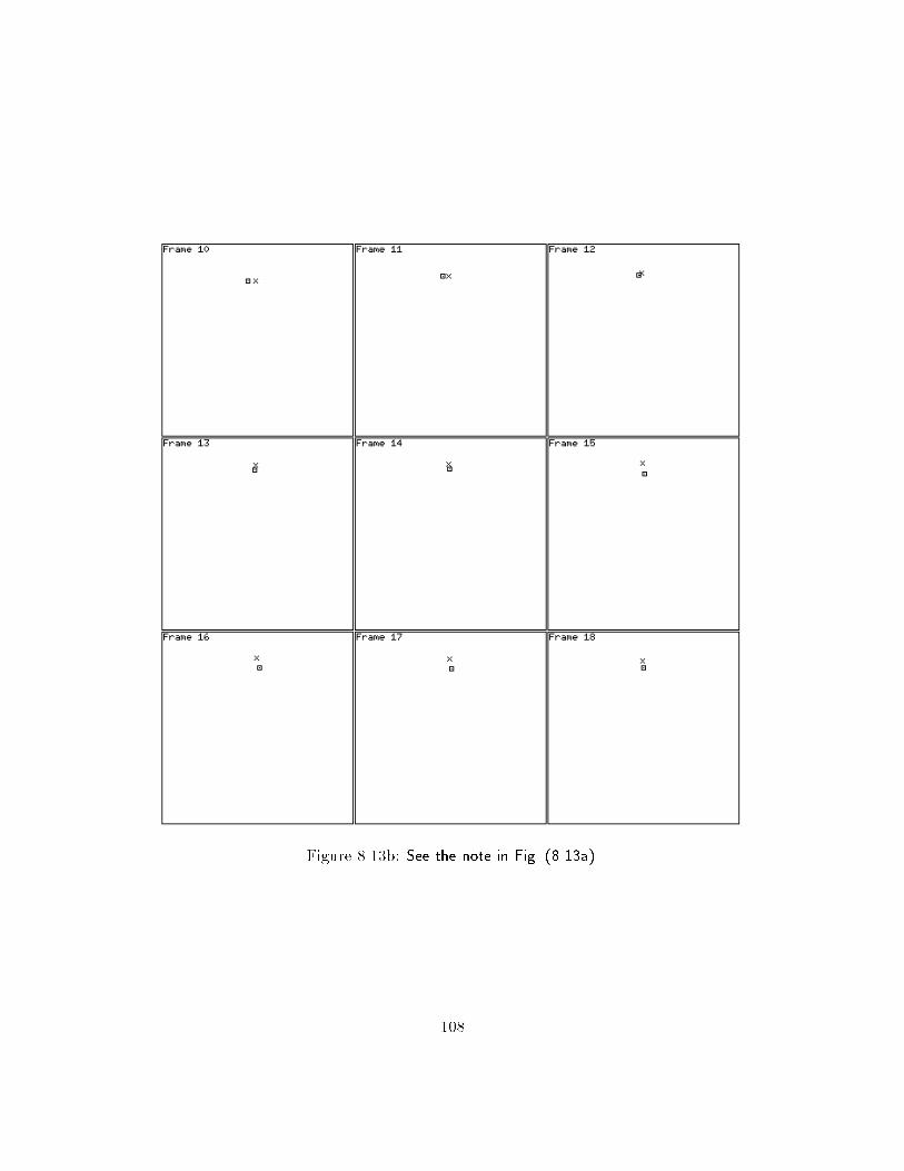
Figure 8.13b: See the note in Fig. (8.13a).
108
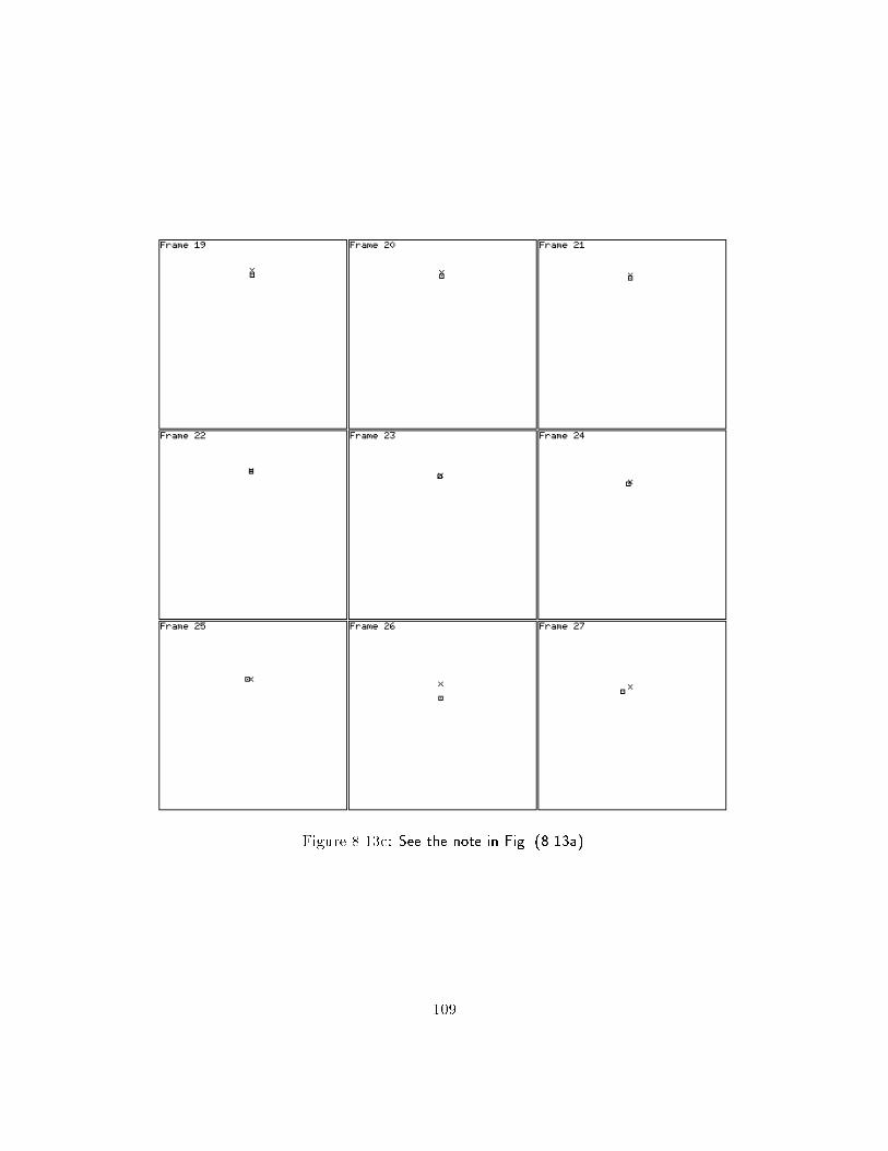
Figure 8.13c: See the note in Fig. (8.13a).
109
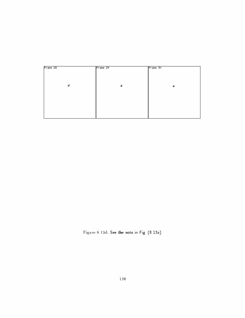
Figure 8.13d: See the note in Fig. (8.13a).
110
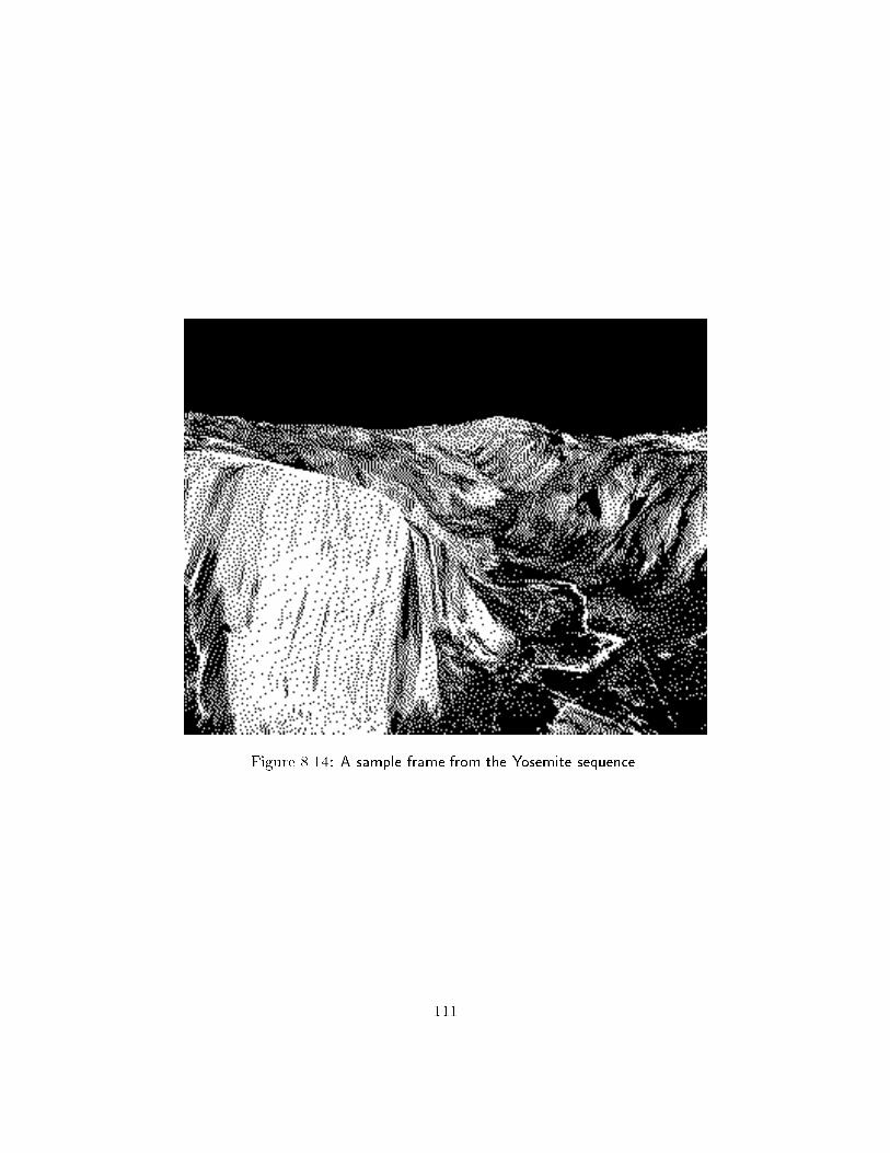
Figure 8.14: A sample frame from the Yosemite sequence.
111
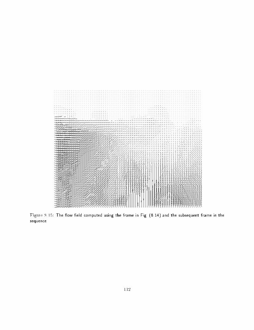
Figure 8.15: The ow �eld computed using the frame in Fig. (8.14) and the subsequent frame in thesequence.
112
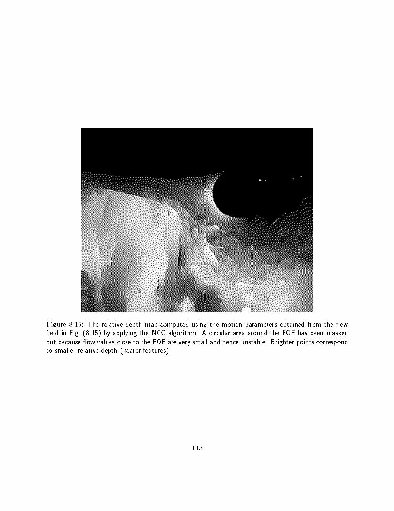
Figure 8.16: The relative depth map computed using the motion parameters obtained from the ow�eld in Fig. (8.15) by applying the NCC algorithm. A circular area around the FOE has been maskedout because ow values close to the FOE are very small and hence unstable. Brighter points correspondto smaller relative depth (nearer features).
113
Chapter 9
Conclusions
We presented algorithms to compute the motion parameters of a sensor. Unlike existing alternative
methods, our methods use all available data, qualifying as global methods. These can be expected
to be more robust when compared to local methods that operate on data from a small region of
the image. This is supported by experimental results that were shown in this thesis.
The ow circulation algorithm computes the rotational parameters. It is based on the observa-
tion that the curl of the vector optical ow �eld is linear in the rotational parameters. Instead of
using the curl values, equivalently, we make use of circulation values which are contour integrals on
the image plane. The parameters of the linear �t are declared to be the rotational velocities. The
algorithm is approximate, in that the curl values are composed of not just the linear terms from
the rotational parameters, but also contain contribution from the translational parameters. The
e�ect of the translational terms is nulli�ed for pure rotation and for frontal planar surfaces; under
such conditions, the linearity is exact and we obtain the correct rotational parameters (for no-noise
situations). Under other conditions, the linearity is only approximate, and the approximation is
expected to hold well in a global sense; i.e., if we use data from all over the image, we expect the
deviations from the linearity to cancel out under typical circumstances.
From the experiments, we �nd that this is indeed the case. We obtained very accurate results for
ow �elds simulated using range data (of non-planar objects), even in the presence of translation.
Using ow �elds computed from a real image sequence (taken from an aircraft), we obtained
quite accurate estimates for the angular velocity. We observe from our derivations and from the
experiments that the algorithm is exact for pure rotation, and is globally approximate for typical
situations. The algorithm is very easy to implement because of the simplicity of the computations.
Integrating along square contours is particularly simple if a dense ow �eld is available on the
cartesian image plane. Note however, that it is su�cient to obtain a few measurements of the curl
value from areas of the image with the same relative motion parameters. This could conceivably be
done by feature detectors measuring circulation. The results from the noise experiments suggest
that the performance of the algorithm degrades gracefully with respect to noise, starting with zero
error in the case of pure rotation.
114
The FOE search algorithms are also easily understood. For candidate FOEs, circular component
functions are computed; the projection of the circular component function on suitable spaces leaves
behind a residual function whose norm is a measure of the correctness of the choice of the FOE. In
particular, for the correct choice of the FOE, this norm is zero, and is non-zero for the other choices.
We provide several methods to perform this computation. Of particular interest are the methods
that exploit the known (quadratic) shape of the error surface in order to simplify the algorithms.
As a result, the center-surround kernel and the quadratic polynomial projection method involve no
search; we need to do the residue computation only for six choices of the FOE. The correct FOE is
obtained by a simple computation (a linear system solution).
The algorithms perform well on synthetic and real data. For the noise models treated here,
the degradation with increasing noise magnitude is smooth. The quadratic polynomial projection
method performs better than the center-surround kernel method. The NCC algorithm performs
better than either of these if there is little or no rotational velocity. This can be seen from the
results from both synthetic and real data. The subspace projection method involves searching
and so is not as computationally e�cient as the other methods. Also, in the experiments on real
images, the quadratic polynomial projection method seems to perform as well as the subspace pro-
jection method. The center-surround kernel method, even though fast, does not do well on real
image sequences possibly because of its local derivative operation. Thus, the quadratic polyno-
mial projection method seems to be a good compromise since it is fast and quite accurate. For
sequences where motion is known to be predominantly translational, the method of choice is the
NCC algorithm because it is the fastest one and is the most accurate for such sequences.
For the methods presented in this thesis, we have assumed that the optical ow �eld is given to
us. For the experiments with real image sequences, we used available code to do the computation.
Often, the optical ow �eld was very noisy. Obtaining noise-free optical ow �elds is still an elusive
issue and is provably impossible to obtain in many situations, due to the aperture problem. Any
advances in better computation methods for optical ow �elds will directly bene�t the algorithms
presented in this thesis.
In the methods presented in this thesis, we have ignored certain issues of visual motion analysis.
We mention them here. The judgement of egomotion and scene structure does not necessarily have
to be obtained exclusively from the optical ow �eld. Correspondence of features is also a powerful
clue to self-motion and structure. Also, the analysis here has been implicitly restricted to two-frame
motion. It is possible to consider several frames at once, not merely to obtain a reliable optical
ow (as attempted by Heeger [22], for example), but integration of information across time by
the use of techniques such as Kalman �ltering might be necessary to reduce the noise-sensitivity
of the computations. Future work in visual motion analysis should consider integration of the
di�erent sources of information, arising from modalities such as optical ow and correspondence
and temporal consistency. Other useful techniques that are likely to simplify motion analysis include
tracking, active vision, and qualitative vision.
115
There is also a need to study the confounding parameters problem. As discussed in Chapter 6,
there is an interplay between the rotational parameters and the translational parameters. The
e�ect is worsened when the �eld of view is small or when the entire scene consists of planar or
nearly-planar structures. This is an issue that a�ects not only the algorithms presented here; all
the algorithms that exist to do motion parameter estimation or structure from motion are plagued
by this issue. It would be useful to �nd a di�erent set of motion parameters which does not su�er
from this problem of interaction between parameters.
116
Bibliography
[1] E.H. Adelson and J.R Bergen. Spatiotemporal energy models for the perception of motion.Journal of the Optical Society of America A, 2:284{299, 1985.
[2] G. Adiv. Determining three-dimensional motion and structure from optical ow generatedby several moving objects. IEEE Transactions on Pattern Analysis and Machine Intelligence,7:384{401, 1985.
[3] J. K. Aggarwal and N. Nandhakumar. On the compuation of motion from sequences of images{a review. Proceedings of the IEEE, 76(8):917{935, August 1988.
[4] J. Aloimonos, I. Weiss, and A. Bandyopadhyay. Active vision. International Journal of Com-puter Vision, 1:333{356, 1988.
[5] P. Anandan. A computational framework and an algorithm for the measurement of visualmotion. International Journal of Computer Vision, 2:283{310, 1989.
[6] S.T. Barnard and W.B. Thompson. Disparity analysis of images. IEEE Transactions onPattern Analysis and Machine Intelligence, 2:333{340, 1980.
[7] J. L. Barron, D. J. Fleet, and S. S. Beauchemin. Performance of optical ow techniques.Technical Report RPL-TR-9107, Robotics and Perception Laboratory, Queens University,Kingston, Ontario, Canada, July 1992. Also as TR No. 299, Dept. of Comp. Sci., U of WesternOntario.
[8] P. Bouthemy. A maximum-likelihood framework for determining moving edges. IEEE Trans-actions on Pattern Analysis and Machine Intelligence, 11(5):499{511, May 1989.
[9] W. Burger and B. Bhanu. Estimating 3-d egomotion from perspective image sequences.IEEE Transactions on Pattern Analysis and Machine Intelligence, 12(11):1040{1058, Novem-ber 1990.
[10] P. Burt and E.H. Adelson. The laplacian pyramid as a compact image code. IEEE Transac-tions on Communications, 31:532{540, 1983.
[11] P.J. Burt. Fast algorithms for estimating local image properties. Computer Vision, Graphicsand Image Processing, 21:368{382, 1983.
[12] M. Fahle and T. Poggio. Visual hyperacuity: Spatio-temporal interpolation in human vision.Proceedings of the Royal Society of London B 213, B 213:451{477, 1981.
[13] F. Faugeras, O.D. Lustman and G. Toscani. Motion and structure from point and line matches.In Proc. of the First International Conference on Computer Vision, 1987.
117
[14] D. Fleet. Personal communication, 1992.
[15] D. J. Fleet and A. D. Jepson. Computation of component image velocity from local phaseinformation. International Journal of Computer Vision, 5:77{104, 1990.
[16] J. J. Gibson. The Perception of the Visual World. The Riverside Press, Cambridge, Mass,1950.
[17] J. J. Gibson, P. Olum, and F. Rosenblatt. Parallax and perspective during aircraft landings.American Journal of Psychology, 68:372{385, 1955.
[18] N. M. Grzywacz and A. L. Yuille. A model for the estimate of local image velocity by cells inthe visual cortex. Proc. Royal Soc. Lond. A, 239:129{161, 1990.
[19] D. Heeger and A. Jepson. Simple method for computing 3d motion and depth. In Proceed-ings of the 3rd International Conference on Computer Vision, pages 96{100, Osaka, Japan,December 1990.
[20] D. Heeger and A. Jepson. Visual perception of 3d motion. Neural Computation, 2:127{135,1990.
[21] D. Heeger and A Jepson. Subspace methods for recovering rigid motion i: Algorithm andimplementation. Research in Biological and Computational Vision Tech Rep RBCV-TR-90-35, University of Toronto, 1991.
[22] D. J. Heeger. Optical ow using spatiotemporal �lters. International Journal of ComputerVision, 1:279{302, 1988.
[23] D. J. Heeger and A. Jepson. Visual perception of three-dimensional motion. MIT Medialaboratory technical report 124, Massachusetts Institute of Technology, December 1989.
[24] D. J. Heeger and A. D. Jepson. Subspace methods for recovering rigid motion i: Algorithmand implementation. International Journal of Computer Vision, 7(2):95{117, 1992.
[25] F. Heitz and P. Bouthemy. Multimodal estimation of discontinuous optical ow using markovrandom �elds. Technical report, IRISA/INRIA, Campus Universitaire de Beaulieu, 35042-Rennes Cedex, France, 1990.
[26] F. B. Hildebrand. Advanced Calculus for Applications. Prentice-Hall, Inc, Englewood Cli�s,New Jersey, 1962.
[27] E.C Hildreth. Computations underlying the measurement of visual motion. Arti�cial Intelli-gence, 23:309{354, 1984.
[28] B. K. P. Horn and E. J. Weldon. Direct methods for recovering motion. International Journalof Computer Vision, 2:51{76, 1988.
[29] B.K.P Horn. Robot Vision. The MIT Press, 1987.
[30] B.K.P Horn and B.G Schunk. Determining optical ow. Arti�cial Intelligence, 17:185{203,1981.
[31] R. Hummel and V. Sundareswaran. Motion parameter estimation from global ow �eld data.IEEE Transactions on Pattern Analysis and Machine Intelligence, to appear.
118
[32] A. Jepson and D. Heeger. Subspace methods for recovering rigid motion ii: Theory. Researchin Biological and Computational Vision Tech Rep RBCV-TR-90-36, University of Toronto,1991.
[33] C. Jerian and R. Jain. Polynomial methods for structure from motion. IEEE Transactions onPattern Analysis and Machine Intelligence, 12:1150{1166, 1990.
[34] G. Johansson. Visual motion perception. Scienti�c American, 232:76{88, 1975.
[35] J. J. Koenderink. Some theoretical aspects of optic ow. In Rik Warren and Alexander H.Wertheim, editors, Perception and control of self-motion, chapter 2, pages 53{68. LawrenceErlbaum Associates, Hillsdale, New Jersey, 1990.
[36] J. J. Koenderink and A. J. Van Doorn. Invariant properties of the motion parallax �eld dueto the movement of rigid bodies relative to an observer. Optica Acta, 22(9):773{791, 1975.
[37] J. J. Koenderink and A. J. Van Doorn. Local structure of movement parallax of the plane.Journal of the Optical Society of America, 66(7), 1976.
[38] J. J. Koenderink and A. J. Van Doorn. Exterospeci�c component of the motion parallax �eld.Journal of the Optical Society of America, 71(8):953{957, 1981.
[39] D. Lawton. Processing translational image sequences. Computer Vision, Graphics and ImageProcessing, 22:116{144, 1983.
[40] J. R. Lishman and D. N. Lee. The autonomy of visual kinaesthesis. Perception, 2:287{294,1973.
[41] H.C. Longuet-Higgins. A computer algorithm for reconstructing a scene from two projections.Nature, 293:133{135, 1981.
[42] H.C. Longuet-Higgins. The visual ambiguity of a moving plane. Proc. Royal Soc. Lond. B,223:165{175, 1984.
[43] H.C. Longuet-Higgins and K. Prazdny. The interpretation of a moving retinal image. Proc.Royal Soc. Lond. B, 208:385{397, 1980.
[44] B. D. Lucas and T. Kanade. An iterative image registration technique with an application tostereo vision. In Proc. 7th Intern. Joint Conference on AI, pages 674{679, Vancouver, 1981.
[45] S. J. Maybank. Algorithm for analysing optical ow based on the least-squares method. Imageand Vision Computing, 4:38{42, 1986.
[46] S. J. Maybank. A Theoretical Study of Optical ow. PhD thesis, University of London, 1987.
[47] A. Mitiche, R. Grisell, and J.K. Aggarwal. On the smoothness of a vector �eld{application tooptical ow. IEEE Transactions on Pattern Analysis and Machine Intelligence, 10(6):943{949,1988.
[48] H.P. Moravec. Towards automatic visual obstacle avoidance. In Proc. 5th International JointConference on Arti�cial Intelligence, page 584, 1977.
[49] H. H. Nagel. On the estimation of optical ow: relations between di�erent approaches andsome new results. Arti�cial Intelligence, 33:299{324, 1987.
119
[50] K. Nakayama. Biological image motion processing: A review. Vision Research, 25:625{660,1985.
[51] K. Nakayama and J. Loomis. Optical velocity patterns, velocity-sensitive neurons, and spaceperception: a hypothesis. Perception, 3:63{80, 1974.
[52] S. Negahdaripour and B. K. P. Horn. A direct method for locating the focus of expansion.Computer Vision, Graphics and Image Processing, 46:303{326, 1989.
[53] K. Prazdny. Egomotion and relative depth from optical ow. Biological Cybernetics, 36:87{102, 1980.
[54] K. Prazdny. Determining the instantaneous direction of motion from optical ow generated bya curvilinearly moving observer. Computer Vision, Graphics and Image Processing, 17:238{248, 1981.
[55] K. Prazdny. On the information in optical ows. Computer Vision, Graphics and ImageProcessing, 22:239{259, 1983.
[56] D. Regan and K. I. Beverley. Visual responses to vorticity and the neural analysis of optic ow. Journal of the Optical Society of America A, 2(2):280{283, February 1985.
[57] J. H. Rieger and D. T. Lawton. Processing di�erential image motion. Journal of the OpticalSociety of America A, 2:354, 1985.
[58] I. Rigoutsos. Massively parallel Bayesian object recognition. PhD thesis, New York University,New York, Aug 1992.
[59] A. Rosenfeld and A.C. Kak. Digital Picture Processing. Academic Press, New York, 1976.
[60] R. Schalko�. Digital Image Processing and Computer Vision. John Wiley, 1989.
[61] I.K. Sethi and R. Jain. Finding trajectories of feature points in a monocular image sequence.IEEE Transactions on Pattern Analysis and Machine Intelligence, 9:56{73, January 1987.
[62] E.P. Simoncelli, E. H. Adelson, and D. J. Heeger. Probability distributions of optical ow. InProc. Computer Vision and Patter Recognition, pages 310{315, Maui, Hawaii, June 1991.
[63] M. W. Spong and M. Vidyasagar. Robot Dynamics and Control. John Wiley & Sons, 1989.
[64] G. Strang. Linear Algebra and its Applications. Harcourt Brace Jovanovich, San Diego, thirdedition, 1988.
[65] M. Subbarao and A. Waxman. On the uniqueness of image ow solutions for planar surfacesin motion. Computer Vision, Graphics and Image Processing, 36:208{228, 1986.
[66] V. Sundareswaran. Egomotion from global ow �eld data. In IEEE Workshop on VisualMotion, pages 140{145, Princeton, New Jersey, Oct 1991.
[67] V. Sundareswaran. A fast method to estimate sensor translation. In Proceedings of the SecondEuropean Conference on Computer Vision, Santa Margherita, Italy, May 1992.
[68] V. Sundareswaran and R. Hummel. Motion parameter estimation using the curl of the ow�eld. In Eighth Israeli Conference on AI and Computer Vision, Tel-Aviv, Dec 1991.
120
[69] K. Tanaka and Hide-Aki Saito. Analysis of motion of the visual �eld by direction, expan-sion/contraction, and rotation cells clustered in the dorsal part of the medial superior temporalarea of the macaque monkey. Journal of Neurophysiology, 62(3):626, September 1989. Alsosee page 642.
[70] C. Tomasi and T. Kanade. Factoring image sequences into shape and motion. In IEEEWorkshop on Visual Motion, pages 21{28, Princeton, New Jersey, Oct 1991.
[71] R. Tsai and T. Huang. Uniqueness and estimation of three-dimensional motion parametersof rigid bodies with curved surfaces. IEEE Transactions on Pattern Analysis and MachineIntelligence, 6:13{27, 1984.
[72] S. Ullman. The interpretation of visual motion. M. I. T. Press, Cambridge, 1979.
[73] S. Ullman. Analysis of visual motion by biological and computer systems. Computer, 14(8):57{69, 1981.
[74] A. Verri and T. Poggio. Motion �eld and optical ow: Qualitative properties. IEEE Transac-tions on Pattern Analysis and Machine Intelligence, 11:490{498, 1989.
[75] H. von Helmholtz. Handbuck der Physiologischen Optik. Verlag von Leopold Voss, Hamburg,1896. Translation published by Dover Press.
[76] H. Wallach and D.N. O'Connell. The kinetic depth e�ect. Journal of Experimental Psychology,45:205{217, 1953.
[77] A. Waxman, B. Kamgar-Parsi, and M. Subbarao. Closed form solutions to image ow equa-tions. In Proc. of the First International Conference on Computer Vision, pages 12{24, Lon-don, 1987.
[78] A. Waxman and S. Ullman. Surface structure and 3-d motion from image ow: A kinematicanalysis. International Journal of Robotics Research, 4(3):72{94, 1985.
[79] A. Waxman and K. Wohn. Contour evolution, neighborhood deformation, and global image ow: Planar surfaces in motion. International Journal of Robotics Research, 4:95{108, 1985.
[80] T.S. Weng, J. Huang and N. Ahuja. Motion and structure from two perspective views: Al-gorithms, error analysis and error estimation. IEEE Transactions on Pattern Analysis andMachine Intelligence, 11:451{476, 1989.
[81] P. Werkhoven and J. J. Koenderink. Extraction of motion parallax structure in the visualsystem i. Biological Cybernetics, 63:185{191, 1990. Also see pages 193{199.
[82] K. Wohn and A. Waxman. The analytic structure of image ows: deformations and segmen-tation. Computer Vision, Graphics and Image Processing, 49:127{151, 1990.
121