Global monitoring of terrestrial chlorophyll ﬂuorescence ... · of GOME-2 is to make measurements of atmospheric trace gases. While not optimal for ﬂuorescence measurements ow-ingtoitsrelativelylargegroundfootprintandmoderatespec-

Atmos. Meas. Tech., 6, 2803–2823, 2013www.atmos-meas-tech.net/6/2803/2013/doi:10.5194/amt-6-2803-2013© Author(s) 2013. CC Attribution 3.0 License.

Atmospheric Measurement

TechniquesO

pen Access

Global monitoring of terrestrial chlorophyll fluorescence frommoderate-spectral-resolution near-infrared satellite measurements:methodology, simulations, and application to GOME-2J. Joiner1, L. Guanter2, R. Lindstrot2, M. Voigt2, A. P. Vasilkov3, E. M. Middleton1, K. F. Huemmrich4, Y. Yoshida3,and C. Frankenberg51NASA Goddard Space Flight Center, Greenbelt, MD, USA2Free University of Berlin, Berlin, Germany3Science Systems and Applications, Inc., Lanham, MD, USA4University of Maryland, Baltimore County, Joint Center for Environmental Technology (UMBC-JCET),Baltimore, MD, USA5Jet Propulsion Laboratory, California Institute of Technology, Pasadena, CA, USA

Correspondence to: J. Joiner ([email protected])

Received: 23 March 2013 – Published in Atmos. Meas. Tech. Discuss.: 22 April 2013Revised: 15 August 2013 – Accepted: 4 September 2013 – Published: 25 October 2013

Abstract. Globally mapped terrestrial chlorophyll fluores-cence retrievals are of high interest because they can provideinformation on the functional status of vegetation includ-ing light-use efficiency and global primary productivity thatcan be used for global carbon cycle modeling and agricul-tural applications. Previous satellite retrievals of fluorescencehave relied solely upon the filling-in of solar Fraunhofer linesthat are not significantly affected by atmospheric absorption.Although these measurements provide near-global coverageon a monthly basis, they suffer from relatively low preci-sion and sparse spatial sampling. Here, we describe a newmethodology to retrieve global far-red fluorescence infor-mation; we use hyperspectral data with a simplified radia-tive transfer model to disentangle the spectral signatures ofthree basic components: atmospheric absorption, surface re-flectance, and fluorescence radiance. An empirically basedprincipal component analysis approach is employed, primar-ily using cloudy data over ocean, to model and solve forthe atmospheric absorption. Through detailed simulations,we demonstrate the feasibility of the approach and showthat moderate-spectral-resolution measurements with a rela-tively high signal-to-noise ratio can be used to retrieve far-redfluorescence information with good precision and accuracy.The method is then applied to data from the Global OzoneMonitoring Instrument 2 (GOME-2). The GOME-2 fluores-

cence retrievals display similar spatial structure as comparedwith those from a simpler technique applied to the Green-house gases Observing SATellite (GOSAT). GOME-2 en-ables global mapping of far-red fluorescence with higher pre-cision over smaller spatial and temporal scales than is possi-ble with GOSAT. Near-global coverage is provided within afew days. We are able to show clearly for the first time phys-ically plausible variations in fluorescence over the course ofa single month at a spatial resolution of 0.5◦ × 0.5◦. We alsoshow some significant differences between fluorescence andcoincident normalized difference vegetation indices (NDVI)retrievals.

1 Introduction

Vegetation releases unused absorbed photosynthetically ac-tive radiation primarily as heat with a small amount re-emitted as fluorescence. Measurements of terrestrial chloro-phyll fluorescence are directly related to photosyntheticfunction, and are potentially useful for forest and agri-cultural applications as well as assessment of the terres-trial carbon budget by providing more accurate estimates ofgross primary productivity (GPP) (e.g., Lichtenthaler, 1987;Saito et al., 1998; Corp et al., 2003, 2006; Campbell et al.,

Published by Copernicus Publications on behalf of the European Geosciences Union.

https://ntrs.nasa.gov/search.jsp?R=20140012652 2018-06-03T21:14:22+00:00Z

2804 J. Joiner et al.: O2 A-band fluorescence retrievals

2008; Damm et al., 2010; Joiner et al., 2011, 2012; Franken-berg et al., 2011b; Guanter et al., 2012). Studies show that inhigh light conditions, such as in the late morning and earlyafternoon, when many satellite measurements are made andwhen plants are under stress, fluorescence is correlated tothe amount of absorbed photosynthetically active radiation(APAR) and the efficiency of the plants to utilize this lightto drive photosynthesis (light-use efficiency or LUE) (e.g.,Flexas et al., 2002; Louis et al., 2005; Meroni et al., 2008;Amoros-Lopez et al., 2008; van der Tol et al., 2009; Zarco-Tejada et al., 2009, 2013; Daumard et al., 2010).Fluorescence information is also complementary to

reflectance-based spectral vegetation indices (Meroni andColombo, 2006; Middleton et al., 2008, 2009; Rascher et al.,2009; Meroni et al., 2008; Daumard et al., 2010; Guanteret al., 2007, 2012; Zarco-Tejada et al., 2009, 2013; Joineret al., 2011, 2012; Frankenberg et al., 2011b). For example,popular greenness-based indices such as the normalized dif-ference and enhanced vegetation indices (NDVI and EVI, re-spectively) are linked to chlorophyll content and are relatedto potential photosynthesis, whereas fluorescence should bean indicator of actual photosynthesis. The photochemical re-flectance index (PRI) is sensitive to the de-epoxidation stateof pigments within xanthophyll cycle, a protection mech-anism that evolved in parallel to fluorescence to dissipateexcess energy (Gamon et al., 1992).Knowledge of global chlorophyll fluorescence emissions

is also important for retrievals of trace-gas concentrationsincluding CO2 that require very high accuracy and preci-sion. The emission occurs within the O2 A-band that isused to estimate photon path lengths for these measure-ments. If not properly accounted for, fluorescence emis-sion may produce significant errors in these retrievals(Frankenberg et al., 2012). The effect of fluorescence on anaerosol plume height retrieval from the O2 A-band has alsobeen investigated using a linear error analysis with simulateddata (Sanders and de Haan, 2013).One means of measuring the small fluorescence signal

from passive remote sensing instrumentation is to make useof dark features in the Earth’s reflected spectrum, either fromtelluric absorption or deep solar Fraunhofer lines. For ex-ample, ground-, aircraft-, and space-based approaches haveutilized filling-in of the dark and spectrally wide O2 A-band (∼ 760 nm) and O2 B-band (∼ 690 nm) atmosphericabsorption features to detect the weak fluorescence signal(see, e.g., Guanter et al., 2007; Meroni et al., 2009, 2010).The spectral location of these oxygen absorption features aswell as other absorption bands and solar Fraunhofer linesare shown in Fig. 1 along with the broadband red and far-red fluorescence emission features that peak near 685 and740 nm, respectively.Deep solar Fraunhofer lines have also been used to de-

tect fluorescence from vegetation following the early workof, e.g., Plascyk and Gabriel (1975). Joiner et al. (2011,2012), Frankenberg et al. (2011b), and Guanter et al. (2012)

680 700 720 740 760 780Wavelength (nm)

0.0

0.5

1.0

1.5

2.0

Sca

led

sign

al (

Arb

itrar

y U

nits

)

Reflected RadianceFluorescenceTOA Solar IrradianceAtmospheric Transmittance

Fig. 1. Simulated solar-induced terrestrial fluorescence, typical sim-ulated atmospheric transmittance and reflectance, and solar irradi-ance as a function of wavelength computed for an instrument withFWHM= 0.3 nm. The fluorescence shows red and far-red chloro-phyll emission features with peaks near 685 and 740 nm, respec-tively. Oxygen A and B absorption bands are located near 687 and760 nm, respectively, while water vapor absorption is shown overa broad spectral range between about 690 and 740 nm. The solar ir-radiance shows weak solar Fraunhofer line structure at this spectralresolution.

used near-infrared (NIR) solar Fraunhofer lines, which arefilled in by vegetation fluorescence, to globally map terres-trial fluorescence with the high-spectral-resolution interfer-ometer aboard the Japanese Greenhouse gases ObservingSATellite (GOSAT). Joiner et al. (2012) strongly suggestedthat fluorescence may also be measurable from space withlower-spectralresolution instrumentation as compared withthe GOSAT interferometer or similar instruments. They fo-cused on filling-in of the 866 nm Ca II solar Fraunhofer lineas measured with the SCanning Imaging Absorption spec-troMeter for Atmospheric CHartographY (SCIAMACHY)satellite instrument. This filling-in appears to be produced byfluorescence from chlorophyll as supported by Gamon andBerry (2012). The SCIAMACHY spectral resolution at thiswavelength is about 0.5 nm.While the current satellite results show promise for use in

estimation of GPP, the GOSATmeasurements have fairly lowspatial sampling and relatively low single-observation preci-sion (Joiner et al., 2011; Frankenberg et al., 2011a; Guanteret al., 2012). The SCIAMACHY results have higher sam-pling frequency, but the very low signal levels spectrally farfrom the far-red fluorescence peak also result in low pre-cision for single observations (Joiner et al., 2012). To pro-duce global maps with high enough fidelity for comparisonswith other measurements and models, GOSAT and SCIA-MACHY fluorescence retrievals must be averaged spatiallyand/or temporally. In doing so for GOSAT, there can bea substantial sampling or representativeness error introducedby the averaging of sparse observations within a relativelylarge grid box.

Atmos. Meas. Tech., 6, 2803–2823, 2013 www.atmos-meas-tech.net/6/2803/2013/

J. Joiner et al.: O2 A-band fluorescence retrievals 2805

Other approaches for satellite fluorescence retrievals haveaimed at utilization of the strong atmospheric oxygen bands(A and B bands) that absorb at wavelengths where chloro-phyll fluorescence is emitted. For example, approaches toseparate fluorescence features from those of reflectance forspace-based measurements have been developed in which at-mospheric absorption is assumed to be perfectly modeled(e.g., Mazzoni et al., 2008, 2010, 2012). More complex al-gorithms have been proposed and tested on simulated data inwhich the parameters affecting O2 absorption are retrievedand accounted for using a radiative transfer model (Guan-ter et al., 2010). Low- spectral-resolution O2 A-band satellitemeasurements from the MEdium Resolution Imaging Spec-trometer (MERIS) aboard Envisat have also been used to re-trieve information about fluorescence (Guanter et al., 2007).Thus far, these satellite measurements are spatially and tem-porally limited and require an on-ground nearby nonfluoresc-ing reference target for normalization.Here, we develop new methodology to retrieve the far-

red chlorophyll fluorescence using space-based hyperspec-tral measurements in and around the O2 A-band. Instead ofexclusively using the filling-in of solar Fraunhofer lines asin the previous works with GOSAT and SCIAMACHY, wedemonstrate that fluorescence can be retrieved by exploit-ing the different spectral structure produced by the far-redchlorophyll fluorescence feature (including both solar andtelluric line filling), atmospheric absorption, and surface re-flectance.Our methodology is similar to approaches developed for

ground-based instrumentation (Guanter et al., 2013) in thatradiative transfer in atmospheric absorption bands is ap-proximated statistically using a principal component anal-ysis (PCA) (or singular value decomposition, SVD). SVDapproaches have also been applied to satellite fluorescenceretrievals using wavelengths not affected by atmospheric ab-sorption (Guanter et al., 2012). In this work, we expand theuse of PCA to include the geometry of a space-based in-strument for wavelengths where significant atmospheric ab-sorption takes place. This scenario is more complex than forground-based measurements. Fluorescence emission can besignificantly absorbed in the atmosphere. Because this ab-sorption is different in magnitude from that of reflected sun-light, the scenario for a satellite retrieval is more difficult ascompared with that for a ground-based instrument. While ourapproach does not require a nearby nonfluorescing target asin other techniques, a representative sample of observationsover nonfluorescing scenes is needed in order to generate acomprehensive set of PCs. For this purpose, we use cloudyobservations over ocean covering a large range of latitudeson a daily basis.We conduct simulations to demonstrate the applicability of

our approach to current and proposed satellite instruments.We then apply our technique to data from the Global OzoneMonitoring Instrument 2 (GOME-2). The primary functionof GOME-2 is to make measurements of atmospheric trace

gases. While not optimal for fluorescence measurements ow-ing to its relatively large ground footprint and moderate spec-tral resolution, its high sampling and signal-to-noise ratioenable state-of-the-art fluorescence retrievals in the far-redchlorophyll emission feature. Near-global coverage is pro-vided within a few days from GOME-2 measurements witha high signal-to-noise ratio. Accurate and frequent measure-ments from GOME-2 will lead to a fluorescence data set withunprecedented temporal and spatial resolution; this in turnshould enable detailed studies including more direct compar-isons with flux tower measurements.

2 GOME-2 satellite data

In this work, we use data from GOME-2. GOME-2 is anoperational nadir-viewing UV/visible cross-track scanningspectrometer (Munro et al., 2006). It flies as part of the Eu-ropean Meteorological Satellite (EUMETSAT) Polar System(EPS) MetOp mission series. GOME-2 measures the Earth’sbackscattered radiance and the extraterrestrial solar irradi-ance at wavelengths between 240 and 790 nm in four detec-tor channels. Here, we use level 1B data from revision R2 inchannel 4 that cover wavelengths 590–790 nm with a spectralresolution of approximately 0.5 nm (Callies et al., 2000) anda relatively high SNR (> 1000).The nadir Earth footprint size is 40 km× 80 km, and the

nominal swath width is 1920 km. A single GOME-2 in-strument provides global coverage of the Earth’s surface inabout 1.5 days. The first flight of GOME-2 is on MetOp-A,launched 19 October 2006 into a polar orbit with an equa-tor crossing time of 09:30 LT. The second flight, launched17 September 2012 on MetOp-B, is also in a morning orbitbut 180◦ out of phase with the first flight model. As such,one or the other instrument is always making measurementson the sunlit part of the Earth, and near-global daily coverageis achievable.

3 Simulated radiances and irradiances

Because our approach relies on an empirical rather thana physical approach for deriving atmospheric absorption, itis difficult to quantify forward model errors. To accuratelyquantify retrieval errors, we conduct detailed simulationsusing combined atmospheric and vegetation models overa wide range of conditions. We also use simulated data toassess the impact of instrument specifications including thesignal-to-noise ratio (SNR) and spectral resolution on fluo-rescence retrievals. Finally, we test different retrieval scenar-ios, such as various spectral fitting windows and numbers ofretrieved parameters, using the simulated radiances.We simulate top-of-the-atmosphere (TOA) sun-

normalized radiances using the matrix operator model(MOMO) radiative transfer model (Fell and Fischer, 2001;Preusker and Lindstrot, 2009). The radiance calculations

www.atmos-meas-tech.net/6/2803/2013/ Atmos. Meas. Tech., 6, 2803–2823, 2013


720 740 760 780Wavelength (nm)

1150

1200

1250

1300

1350

1400

Sola

r Irra

dian

ce (m

W/m

2 /nm

/sr)

FWHM=0.5nmFWHM=0.3nm

Fig. 2. Simulated solar spectra based on Chance and Kurucz (2010)for different instrumentation showing Fraunhofer line structure(FWHM= 0.5 nm is for a GOME-2-like instrument).

utilize absorption line strengths and widths from the high-resolution atmospheric radiance and transmittance modelcode (HITRAN) 2008 data set (Rothman et al., 2009). Theradiances are computed monochromatically and are sampledat 0.005 nm. They are then multiplied by a solar spectrumsampled in the same way and finally convolved with variousinstrument line shape functions.We use solar data originally sampled at 0.001 nm from

kurucz.harvard.edu/sun/irradiance2005/irradthu.dat, similarto Chance and Kurucz (2010) but more highly sampled. Fig-ure 2 shows simulated solar spectra generated for differentinstrument specifications including a spectral resolution sim-ilar to GOME-2 (i.e., full width at half maximum (FWHM)of 0.5 nm sampled at 0.2 nm) and a smaller FWHM of 0.3 nmsampled at 0.1 nm. Significant solar Fraunhofer line structurecan be seen throughout the spectrum with deeper structuresat the higher spectral resolution.Note that we do not simulate the effects of rotational

Raman scattering (RRS) or O2 A-band dayglow emissions.RRS effects are generally small, though not negligible, at thewavelengths of interest (Vasilkov et al., 2013). The effects ofO2 A-band dayglow emissions in the upper atmosphere areexpected to be small (Guanter et al., 2010). Directional ef-fects of the vegetation reflectance and fluorescence are alsonot simulated.Radiances are computed for two view zenith angles

(VZA= 0 and 16◦), four solar zenith angles (SZA= 15◦,30◦, 45◦, 70◦), two atmospheric temperature profiles (mid-dle latitude summer and winter), four surface pressures (955,980, 1005, and 1030 hPa), four values of total column wa-ter vapor (0.5, 1.5, 2.5, and 4.0 cm), five aerosol opticalthicknesses at 550 nm (0.05, 0.12, 0.2, 0.3, and 0.4), andthree aerosol plume heights (700–900, 600–800, and 500–700 hPa) with a continental aerosol model. Two separate datasets are created, one without fluorescence intended for prin-

640 660 680 700 720 740 760 780Wavelength (nm)

0

2

4

6

F s (m

W/m

2 /nm

/sr)

Fig. 3. Canopy-level spectral fluorescence as specified for the rangeof conditions in the simulated data set.

cipal component analyses (henceforth referred to as “train-ing”), and one containing fluorescence intended to examineretrieval performance with the simulated radiances (referredto as “testing”). The training data set uses a spectral libraryof 10 different surface reflectance spectra corresponding tosoil and snow. This provides a total of 38 400 samples in thetraining data set.The testing data set contains surface reflectance and flu-

orescence emission spectra generated with the FluorSAILand FluorMODleaf codes (Jacquemoud et al., 2009; Pe-drós et al., 2010; Miller et al., 2005). A given input leaf-level fluorescence spectrum has been scaled by multiplica-tive factors. Different values of chlorophyll content (from5 to 40 µgcm−2) and leaf area index (from 0.5 to 4) havebeen used for the propagation of the resulting leaf-level flu-orescence spectra to the canopy level. There are 60 distincttop-of-canopy fluorescence spectra from these combinationsas shown in Fig. 3. Top-of-canopy reflectance spectra areconsistently generated by the leaf and canopy codes for thesame combinations of chlorophyll content and leaf area in-dex. Other parameters in the models were set to default val-ues as in Guanter et al. (2010). This gives a total of 230 400different samples in the testing data set.

4 Retrieval methodology

4.1 General approach

The total reflectance ρtot, as a function of wavelength λ, mea-sured by a satellite instrument in the NIR spectral region, canbe approximated using a Lambertian model with emissionfrom fluorescence, i.e.,

ρtot(λ) = ρ0(λ) + ρs(λ)T (λ)T (λ)

1− ρs(λ)ρ(λ)+ πFs(λ)T (λ)

[1− ρs(λ)ρ(λ)]E(λ)cos(θ0), (1)



where ρs(λ) is the surface reflectance, ρ0 is the reflectancecontribution in the absence of surface effects, T is the totalirradiance transmittance (including direct and diffuse com-ponents), T is the spherical transmittance from the surface toTOA, ρ is the spherical reflectance of the atmosphere back tothe surface, θ0 is the solar zenith angle (SZA),E(λ) is the ob-served extraterrestrial solar irradiance, and Fs is the radianceemission from fluorescence at the surface.The basic idea behind our approach is to separate the spec-

tral features related to three basic components: atmosphericabsorption (T and T ), surface reflectivity (ρs), and fluo-rescence radiance (Fs). Assuming that the effects of atmo-spheric scattering are small (i.e., ρ0 � 0 and ρsρ � 1), wemay rewrite Eq. (1) as

ρtot(λ) = ρs(λ)T (λ)T (λ) + πFs(λ)T (λ)

E(λ)cos(θ0), (2)

where T (λ) and T (λ) now include atmospheric molecu-lar absorption only. We now combine T and T into a sin-gle parameter, T2(λ) = T (λ)T (λ), that represents the sun-to-satellite (two-way) atmospheric transmittance. Using

T2(λ) = exp [−A2(λ)]= exp[−Av(λ){sec(θ) + sec(θ0)}], (3)

where θ is the satellite view zenith angle (VZA), andA2 andAv represent the two-way and vertical absorptances, respec-tively, and the upwards absorptance, A, as

A(λ) = Av(λ)sec(θ)

= A2(λ)sec(θ)

sec(θ) + sec(θ0) , (4)

then

T (λ) = exp(ln [T2(λ)] sec(θ)

sec(θ) + sec(θ0))

. (5)

Note that the above equations are strictly valid only formonochromatic radiation. Also note that ρ0, ρ, T , and T ,in the presence of atmospheric scattering and in the absenceof atmospheric molecular absorption, are a spectrally smoothfunction of wavelength. Therefore, when atmospheric scat-tering is present, ρs(λ) and Fs(λ) in Eq. (2) can be thoughtof as effective TOA spectral components of surface re-flectance and fluorescence that have been modified by spec-trally smooth atmospheric scattering; the spectral structure ofρ0 can be incorporated into the components of the first termof Eq. (2).To solve for ρs, Fs, and T2, we assume that

each has a distinct spectral structure. We repre-sent the fluorescence far-red emission, Fs(λ), asa Gaussian function of λ centered at 736.8 nm withσ = 21.2 nm, similar to Subhash and Mohanan (1997) andZarco-Tejada et al. (2000). We further assume that ρs(λ),within our limited spectral fitting window, is spectrally

smooth, and model it as a low-order polynomial in λ. Al-ternative parameterizations for fluorescence and reflectancehave been explored (e.g., Mazzoni et al., 2010, 2012).Previous works suggest that small errors in the prescribedshape of the fluorescence emission have little impact on theestimated peak fluorescence value (Daumard et al., 2010;Fournier et al., 2012; Guanter et al., 2013). We estimate thespectral structure of A2 (or T2) using principal components(PCs) as described below.In principle, our approach may be applied to the entire flu-

orescence emission band shown in Fig. 1 containing both thered and far-red features. Alternatively, different fitting win-dows could be used to estimate fluorescence within smallerwavelength ranges. As a starting point to demonstrate ourapproach, we focus on retrievals of the far-red fluorescence.

4.2 Generation of atmospheric PCs

Radiative transfer in the O2 A-band is complex because theshape of the absorption features depends nonlinearly uponthe surface pressure and albedo as well as the vertical struc-ture of atmospheric temperature and cloud/aerosol particles(e.g., Preusker and Lindstrot, 2009). Absorption by water va-por in the 710–745 nm spectral region also depends uponthese parameters and is similarly complex; though less af-fected by saturated lines, the profile is of course more vari-able. Retrieval algorithms have been developed to retrievesome or all of these parameters using O2 A-band radiances(e.g., Guanter et al., 2007; O’Dell et al., 2012). Other factorssuch as filling-in from rotational Raman scattering are typi-cally not accounted for owing to a high degree of complexityresulting from interactions with Mie scattering and depen-dences on other parameters (Vasilkov et al., 2013). Neglect ofthese effects may produce errors in such algorithms. Instru-mental effects such as nonlinearity also challenge physicallybased approaches used to estimate O2 A-band absorption.Instead of using radiative transfer calculations, we have

developed an empirically based alternative for estimation ofA2 or T2(λ); we represent A2(λ) as a linear combination ofprincipal components (PCs) φi(λ) that can be estimated us-ing simulated or real satellite data, i.e.,

A2(λ) =n∑

i=1aiφi(λ), (6)

where ai are the coefficients of the PCs. Instead of usinglaboratory-measured absorption cross sections, as is typicalin the differential optical absorption spectroscopy (DOAS)approach, we use atmospheric spectra, simulated or mea-sured, to derive the spectral components of absorption.As in the DOAS approach, our method implicitly assumes

that the Beer–Lambert law of weak linear absorption applies,although the PCs may be able to incorporate some featuresof nonlinear absorption. Because this law does not strictlyapply to the O2 A-band, where individual lines may become



Fig. 4. Transmittances derived from the training data set with FWHM=0.5 nm. Colors in the left panel correspond to values of total columnwater vapor (light blue, dark blue, green, and red correspond to 4.0, 2.5, 1.5, and 0.5 cm, respectively) for various combinations of solar andviewing zenith angles; colors on right-hand panel showing O2 A-band absorption correspond to different combinations of solar and viewingzenith angles.

PC % of total: 99.8392(99.6467); cumulative % of total: 99.8392(99.6467)

715 720 725 730 735 740 745Wavelength (nm)

0.000.050.100.15

PC #

1

PC % of total: 0.1301( 0.3244); cumulative % of total: 99.9693(99.9711)

715 720 725 730 735 740 745Wavelength (nm)

-0.10.00.10.2

PC #

2


715 720 725 730 735 740 745Wavelength (nm)

-0.10.00.10.20.3

PC #

3


715 720 725 730 735 740 745Wavelength (nm)

-0.2-0.10.00.10.2

PC #

4

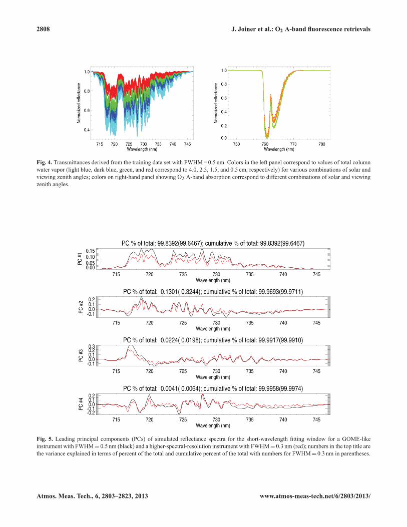
Fig. 5. Leading principal components (PCs) of simulated reflectance spectra for the short-wavelength fitting window for a GOME-likeinstrument with FWHM= 0.5 nm (black) and a higher-spectral-resolution instrument with FWHM= 0.3 nm (red); numbers in the top title arethe variance explained in terms of percent of the total and cumulative percent of the total with numbers for FWHM= 0.3 nm in parentheses.



PC % of total: 99.7792; cumulative % of total: 99.7792

715 720 725 730 735 740 745Wavelength (nm)

0.050.100.15

PC #

1


715 720 725 730 735 740 745Wavelength (nm)

-0.2-0.10.00.1

PC #

2


715 720 725 730 735 740 745Wavelength (nm)

-0.15-0.10-0.050.000.050.10

PC #

3


715 720 725 730 735 740 745Wavelength (nm)

-0.2-0.10.00.1

PC #

4

Fig. 6. Similar to Fig. 5 but the PCA is conducted using actual GOME-2 data taken over ice- and snow-covered surfaces, the Sahara, andcloudy ocean.

optically thick and absorption is temperature dependent, sim-ulations are needed to evaluate how well our simplified ap-proach will work in this spectral region. Our approach is flex-ible in that different fitting windows may be utilized. As willbe shown below, the O2 A-band can in fact be completely re-moved from an extended fitting window without much if anyloss of information content.To the extent that our approach is shown to be success-

ful, there are several advantages. By using PCs, we do notneed to estimate parameters affecting O2 and H2O absorptionsuch as surface pressure, temperature and water vapor pro-files, and cloud and aerosol parameters that affect nearly allsatellite observations. In addition, we eliminate dependenceupon a precise specification of the instrument response func-tion. The PCs may also capture instrument artifacts that areotherwise difficult to quantify.As in DOAS retrievals, we use the logarithm of sun-

normalized radiance spectra for the PCA. We first computePCs with the simulation training data set. For comparison,we also generate PCs using actual GOME-2 satellite radi-ance data. For the GOME-2 PCA, we use spectra from a sin-gle day (1 May 2007) consisting of observations over seaice, snow/ice-covered land, the Sahara, and cloudy ocean forpixels with θo < 75◦. For the cloudy ocean data, we computethe reflectance at 670 nm (ρ670) and use observations only forρ670 > 0.7.

For both real and simulated data, we normalize the spec-tra with respect to a second-order polynomial fit to wave-lengths not significantly affected by atmospheric absorption(i.e., 712–713 and 748–757 nm, and wavelengths > 775 nm)before taking the logarithm of the spectra. This normaliza-tion produces values representative of the total sun to satel-lite absorptance. We are able to use a second-order polyno-mial for this fit of spectra that do not contain complex sur-face reflectances. However, as noted below, we need to usehigher-order polynomials to characterize vegetated surfaces.Alternatively, PCAs may be similarly performed without tak-ing the logarithm of the normalized spectra in order to modeltransmittance instead of absorptance.Absorption affecting fluorescence in the far-red emission

feature includes that from the O2 A-band near 760 nm as wellas a weaker water vapor band at shorter wavelengths. Fig-ure 4 shows examples of normalized spectra approximatingthe sun-to-satellite transmittance separately for two wave-length ranges: (1) 712–747 nm, dominated by H2O absorp-tion, and (2) 747–783 nm encompassing the O2 A-band.Figure 5 shows the leading four PCs for the wave-

length range 712–747 nm computed with simulated data forFWHMs of 0.5 nm (similar to GOME-2) and 0.3 nm. Thespectral variance in this window is due almost exclusivelyto water vapor absorption. The variances explained (withrespect to the total) as well as the cumulative variances



PC % of total: 99.9627(99.9526); cumulative % of total: 99.9627(99.9526)


0.000.050.100.150.200.250.30

PC #

1



-0.4-0.20.00.2

PC #

2



-0.4-0.3-0.2-0.10.00.10.2

PC #

3



-0.4-0.20.00.20.4

PC #

4

Fig. 7. Similar to Fig. 5 but for the long- wavelength fitting window using simulated data.

explained are indicated. The PCs are similar for the two spec-tral resolutions with somewhat deeper structures at the higherresolution. The variance explained by the leading PCs is sim-ilar for the two spectral resolutions.Figure 6 similarly shows PCs generated from actual

GOME-2 satellite data. PCs and variance explained are simi-lar for the simulated and GOME-2 data. The first PC explainsover 99% of the spectral variance, and 99.99% of the vari-ance is captured in the first four modes for both the simulatedand GOME-2 data. However, PC #4 from GOME-2 appearsto correspond to PC #3 from the simulated data, but thereis no similar correspondence between PC #3 from GOME-2and PC #4 from the simulation. The PCs for simulated andreal data are expected to be different as PCs from the real datamay contain information related to instrumental artifacts andprocesses not included in the simulated data (e.g., rotationalRaman scattering). In addition, the simulated data may notrepresent all of the conditions or the distribution of condi-tions that are present in the GOME-2 data, particularly brightscenes that occur over heavily clouded conditions. The train-ing data set, however, does include bright soils and snow.Figures 7 and 8 similarly show the leading PCs for the

spectral window 747–783 nm dominated by strong oxygenA-band absorption near 760 nm. Again, the PCs are similarfor simulated and GOME-2 satellite data with over 99.9%of variance captured by the leading mode, and more than99.999% of the variance explained by the first four modes.

PCs #2 and #3 appear to be reversed for the GOME-2 andsimulated data.

4.3 Solving the nonlinear problem

To solve the nonlinear estimation problem, we use a gradient-expansion algorithm adapted from Marquardt (1963) andBevington (1969). This algorithm provides a relatively fastconvergence, typically 4–6 iterations. We derive and supplyto this algorithm the analytic Jacobians or partial derivativesof the observed radiances with respect to the state variables.Typical Jacobians (i.e., partial derivatives of the re-

flectances with respect to the coefficients of the PCs, sur-face reflectance polynomials, and the peak value of the far-red fluorescence feature at 736.8 nm) are shown in Fig. 10for FWHMs of 0.5 and 0.3 nm. Although the componentsare not completely orthogonal, our simulation results willshow that fluorescence can be successfully disentangled fromatmospheric and surface parameters. Subtle differences inthe Jacobians enable this differentiation. For example, smallFraunhofer structures can be seen in the fluorescence Jaco-bian at wavelengths between about 745 and 758 nm that arenot seen in the other Jacobians. An instrument with a highenough spectral resolution and SNR should be able to detectthese features as will be demonstrated below. Again, deeperspectral structures are seen at the higher spectral resolution.





0.000.050.100.150.200.250.30

PC #

1



-0.2-0.10.00.10.20.3

PC #

2



-0.2-0.10.00.10.20.30.4

PC #

3



-0.4-0.3-0.2-0.10.00.1

PC #

4

Fig. 8. Similar to Fig. 6 but for the long- wavelength fitting window computed using actual GOME-2 data.

��

��

�� !��"�#��$��"%&'�(�)

*��+��,+��-��*.��

"%&'��

��)

��/��0��,��+#��1��+2��3��4*.��0��4��/��-��,+��5��

��2��4�,��

6��/�� 7

��+ ��

8��#��9��0��5��0��

��:

��

Fig. 9. Flow diagram showing the overall processing scheme for GOME-2 fluorescence retrievals.



720 730 740 750 760 770 780Wavelength (nm)

0.00050.00100.00150.00200.0025

Fluo

resc

ence

Jac

.

720 730 740 750 760 770 780Wavelength (nm)

0.20.40.60.81.0

Ref

lect

ivity

con

st. J

ac.

720 730 740 750 760 770 780Wavelength (nm)

-0.04-0.03-0.02-0.010.00

PC#1

Jac

.

Fig. 10. Typical Jacobians (∂ρ/∂x) where x is the far-red fluorescence peak value (top), the wavelength-independent component of thesurface reflectivity (middle), and the coefficient of the first PC (bottom) for FWHM= 0.5 nm (black) and FWHM= 0.3 nm (red). The PCanalyses are carried out separately for the wavelength ranges 712–747 nm and 747–783 nm but are shown in a single plot for convenience.

At convergence, the partial derivatives contained in the Ja-cobian K matrix may be used to compute errors from an un-constrained linear error estimation, i.e.,

Sr =(KT S−1

e K)−1

, (7)

where Sr is the retrieval error covariance matrix, and Se isthe measurement error covariance. We use this approach tocompute fluorescence error standard deviations and correla-tions and compare these error estimates with those obtainedin the full retrieval simulation as will be discussed below. Wealso use the linear approach to estimate errors from GOME-2retrievals.

4.4 Processing of GOME-2 data

The overall processing of GOME-2 data follows the flow di-agram shown in Fig. 9. One subset of radiance data is usedto generate the PCs (chosen such that fluorescence is notpresent), and a different subset is used for the fluorescenceretrievals (data over land). A PCA is conducted daily for eachsubwindow using the daily measured solar flux. We use dataover highly cloudy ocean and snow- and ice-covered surfaces(ρ at 670 nm> 0.7) and the Sahara for the PCA. The derivedPCs are then used for the fluorescence retrieval. Followingthe retrieval, quality assurance checks are done to removehighly cloudy data and failed retrievals as described in moredetail below. Finally, the data are gridded at various tempo-ral resolutions to produce level 3 data sets. More than 5 yr of

720 730 740 750 760 770Wavelength (nm)

0.15

0.20

0.25

0.30

0.35

0.40

Ret

rieve

d su

rface

refle

ctan

ce

Fig. 11. Retrieved spectral surface reflectances for the range of con-ditions in the simulated data set.

GOME-2 data have been processed, and the level 2 data areavailable from http://acdb-ext.gsfc.nasa.gov/People/Joiner/.

4.4.1 GOME-2 fluorescence retrievals

We use a fitting window from 712 to 783 nm for GOME-2retrievals with a fourth-order polynomial to model the sur-face reflectivity and a Gaussian function for the canopy-level far-red fluorescence as described above. We used 25PCs for each of the two PCA subwindows shown above. No



adjustments are made to the calibrated radiances/irradiances;it should be noted that the MetOp-A GOME-2 is known tohave suffered from radiometric degradation over its lifetime.

4.4.2 Cloud filtering and quality control

As in Joiner et al. (2012), we compute the effective cloudfraction fc and eliminate data with fc > 0.4. To computefc, we use the black-sky 16-day gridded filled-land surfacealbedo product from Aqua MODIS (MOD43B3) at 656 nm(Lucht et al., 2000). Application of more or less stringentlimits on cloud contamination within a moderate range (0–0.5) did not substantially alter the derived spatial and tem-poral patterns of Fs, but stricter limits decrease the numberof samples included, and therefore reduce coverage and in-crease noise in the gridded averages.In the results shown below, we include all data passing

gross quality assurance checks on the retrieval convergenceand radiance residuals. These checks removed few obser-vations in general. However, the South Atlantic Anomaly(SAA) adds noise to GOME-2 measurements in the vicin-ity of South America, and most of the data removed by theresidual checks were located in this area. The distribution andsampling frequency of the data used to the generate the PCsleads to higher retrieval uncertainties than the SAA; the rel-atively small number of PCs used in the retrieval generallydoes not capture the highly variable errors found in the re-gion. While many of the affected spectra are screened out byradiance residual checks, the filtering process reduces sam-pling and may not eliminate all affected spectra. Therefore,GOME-2 errors are generally higher over South America ascompared with other areas. We also eliminate all data withSZA> 70◦.

5 Sensitivity analysis

In this section, we retrieve fluorescence using the simulatedradiances for the 230 400 different conditions contained inthe testing data set described in Sect. 3. We conduct retrievalsfor a number of different scenarios. We then compare the re-trieved fluorescence with that of the truth as specified in thetesting data set for the entire sample. Table 1 provides statis-tical results of those comparisons for the scenarios describedbelow.

5.1 Sensitivity to number of PCs used

In the first experiment, we simulate data for a fitting win-dow between 747 and 780 nm and for an instrument withFWHM= 0.5 nm, sampling of 0.2 nm, and SNR= 2000. In-strument noise is uncorrelated between channels, and followsa Gaussian distribution. Here, we use a fourth-order polyno-mial to model the surface reflectivity. Increasing the polyno-mial order does not significantly improve the results, whileuse of a second-order polynomial significantly degrades re-

sults. For reference, Fig. 11 displays the range of spectralsurface reflectances that are retrieved from the diverse simu-lated data.The first four lines of Table 1 show results for retrievals

that use 5, 10, 15, and 25 PCs. There are small biases in allcases with biases generally decreasing with increasing num-bers of PCs. The improvement in both accuracy and precisionis noticeable when increasing from 5 to 10 PCs, and levelsout with further increases. There is virtually no change in theresults when we increase the number of PCs from 25 to 35(not shown). We find that a similar number of PCs is neededfor the shorter-wavelength subwindow (712–747 nm). Forthe remainder of this section, all retrievals will use 25 PCsfor each of the two subwindows.We also computed fluorescence errors using the linear esti-

mation method. Here, we assumed random and uncorrelatedradiance errors. The radiance errors were also assumed to beindependent of wavelength. This is consistent with the errorsgenerated in the simulated data set. We computed errors forthe various wavelength ranges, numbers of PCs, and SNRsused above. We find that the computed fluorescence errorstandard deviations from the linear approach are very close(within ∼ 4%) to those obtained in the full retrieval simula-tion. We find that fluorescence errors can be moderately cor-related with errors in the constant reflectivity term and someof the leading PCs.

5.2 Sensitivity to signal-to-noise ratio

For comparison, Table 1 shows results of fluorescenceretrievals using simulated observations as above withSNR= 1000. Results may be compared with the 25 PCcase (line 4) described in Sect. 5.1 for an instrument withSNR= 2000. Standard deviations and root-mean-squared(RMS) errors for SNR= 1000 are slightly less than twicethose at SNR= 2000. This is consistent with the expectedbehavior of a retrieval based solely on solar Fraunhofer linestructure, where errors are inversely proportional to SNRwith all other parameters held constant (Joiner et al., 2012).

5.3 Sensitivity to the fitting window

In the experiments shown in lines 6–10 of Table 1, we usedifferent fitting windows for an instrument with SNR= 2000and FWHM= 0.5 nm. Fluorescence errors are approximatelya factor of 2 smaller with the 712–747 nm fitting window ascompared with the 747–780 nm shown above. This demon-strates that fluorescence retrievals can be obtained with goodprecision without using the filling-in signal from the O2 A-band. The 712–747 nm window spans the peak far-red fluo-rescence, and also contains H2O absorption. A reduced fit-ting window of 723–747 nm produces slightly degraded re-sults as compared with the 712–747 nm window. Both ofthese shorter-wavelength windows show decreased bias ascompared with the 747–780 nm window that includes the O2



Table 1. Statistical comparison of retrieved versus true values of Fs obtained with the simulated testing data set for different experiments(Exp); all fluorescence radiance units (indicated by *) are mWm−2 nm−1 sr−1. Retrievals are performed for an instrument with a givenfull-width-at-half-maximum (FWHM) line shape function, signal-to-noise ratio (SNR), number of principal components (#PCs), and fittingwindow from starting wavelength λ1 to ending wavelength λ2. Statistics given are the root-mean-squared difference (RMS diff.), correlationcoefficient (r), mean difference (bias) of retrieved minus truth, standard deviation (σ ), and slope (A) and intercept (B) of a linear fit (retrievedfluorescence = A + B · truth) (last two columns).

Exp FWHM SNR #PCs λ1 λ2 RMS diff. r bias σ slope intercept(nm) (nm) (nm) * * * *

1 0.5 2000 5 747 780 0.88 0.67 −0.68 0.57 0.43 −0.032 0.5 2000 10 747 780 0.58 0.82 −0.37 0.45 0.58 0.113 0.5 2000 15 747 780 0.50 0.87 −0.32 0.38 0.72 −0.014 0.5 2000 25 747 780 0.43 0.87 −0.22 0.38 0.80 0.015 0.5 1000 25 747 780 0.70 0.69 −0.22 0.67 0.80 0.016 0.5 2000 25 712 747 0.33 0.97 −0.07 0.32 1.00 0.077 0.5 2000 25 723 747 0.37 0.97 −0.01 0.37 0.94 0.138 0.5 2000 25 755 775 0.56 0.76 −0.30 0.47 0.71 0.019 0.5 2000 25 759 768 1.19 0.43 −0.46 1.10 0.70 −0.1310 0.5 2000 25 747 758 1.48 0.58 −0.03 1.48 0.98 0.0111 0.3 2000 25 747 780 0.49 0.85 −0.29 0.40 0.80 −0.0612 0.3 2000 25 712 747 0.22 0.99 −0.11 0.19 0.94 0.02

1 2 3 4 5True Fs (mW/m2/sr/nm)

1

2

3

4

5

Ret

rieve

d F s

(m

W/m

2 /sr/

nm)

1 2 3 4 5True Fs (mW/m2/sr/nm)

1

2

3

4

5R

etrie

ved

F s (m

W/m

2 /sr/n

m)

Fig. 12. Fluorescence retrievals from simulated data (y axis) using wavelengths between 712 and 747 nm for instruments withFWHM= 0.5 nm (left) and FWHM= 0.3 nm (right), both with a signal-to-noise ratio of 2000. Fluorescence is averaged over the wave-lengths used in the retrieval and compared with the “truth” (x axis) averaged in the same way. Standard deviations are shown with verticalbars. Different symbols are shown for the various values of chlorophyll content, and different colors are for the different values of leaf areaindex.

A-band. Our results are consistent with those of Guanter et al.(2013), who similarly showed that fitting windows in thisspectral region, without the benefit of the O2 A-band, can beused to retrieve fluorescence with higher-spectral-resolutionground-based instruments.Table 1 also examines results for fitting windows more

confined to the O2 A-band. As may be expected, retrievalsare degraded for a smaller fitting window of 755–775 nm ascompared with the 747–780 nm window used above. Resultsare also shown with a smaller fitting window of 759–768 nm.This window consists primarily of the O2 A-band with em-bedded Fraunhofer structure. Note that the strongest solarFraunhofer feature within the range 712–783 nm occurs in-side the O2 A-band region near 766 nm. Results are signif-icantly degraded with this limited fitting window. Franken-

berg et al. (2011a) noted the difficulties associated with dis-entangling fluorescence spectral information from that ofaerosols, clouds, surface pressure, etc., using only wave-lengths within O2 A-band spectral region. Although there isa significant correlation between fluorescence and these otherparameters, there is nevertheless a limited ability to retrieveinformation about fluorescence within this absorption band.However, biases increase as the fitting window is more con-fined to the O2 A-band spectral region. Precision is signifi-cantly degraded with a limited fitting window of 747–758 nmcontaining only weak solar Fraunhofer line structures, whilethe accuracy for this fitting window is good.



750 755 760 765 770 775 780Wavelength (nm)

0.1

0.2

0.3

0.4

0.5

RM

S re

sidu

al (

%) No fit of Fs

Fit Fs

Fig. 13. RMS of simulated radiance residuals (in percent ofradiance) from the testing data set with FWHM= 0.3 nm andSNR= 2000 when fluorescence radiance (Fs) is fitted/retrieved andwhen it is not fitted/retrieved.

5.4 Sensitivity to spectral resolution

In order to show the sensitivity of the results to spectralresolution, we performed a similar set of experiments ata higher spectral resolution (FWHM= 0.3 nm, sampling of0.1 nm) as compared with that used in the above subsec-tions. Lines 12 and 13 of Table 1 show retrieval statistics forthe higher-spectral-resolution instrument with SNR of 2000for fitting windows of 747–780 nm and 712–747 nm, respec-tively. The precision is significantly improved as comparedwith FWHM= 0.5 nm retrievals. This improvement resultsfrom (1) more spectral samples within the fitting window and(2) a larger filling-in fluorescence signal in the cores of thedeeper Fraunhofer lines that are better resolved at the higherspectral resolution as shown in Fig. 10. Further improve-ments can be made by making measurements with higherspectral resolution and/or increased sampling. We also var-ied the fitting window as in Sect. 5.3 for FWHM= 0.3 nm,and reached the same conclusions as with FWHM= 0.5 nm.As described above, there are 60 distinct values of fluo-

rescence (averaged between 740 and 780 nm) ranging fromnear zero to near 4mWm−2 nm−1 sr−1. For each value, theobserving conditions vary (e.g., different SZAs, VZAs, sur-face pressures, temperature profiles, and aerosol parameters).Figure 12 shows retrieval results using the 712–747 nm fit-ting window for the FWHM= 0.3 and 0.5 nm simulated datawith SNR= 2000. This figure shows that biases are moreprevalent for higher levels of fluorescence.

5.5 Radiance residuals from simulated data

Figure 13 shows RMS of the radiance residuals (ob-served minus calculated radiance) for two cases withFWHM= 0.3 nm, SNR= 2000, and a fitting window of 747–

Fig. 14. RMS of GOME-2 radiance residuals obtained with andwithout fitting Fs (in percent of the observed radiance) for a sin-gle day for moderately to highly vegetated pixels.

780 nm: (1) fluorescence is not retrieved, and (2) fluores-cence is retrieved. The RMS of the residual is computed ateach wavelength averaged over all conditions in the simula-tion testing data and shown as a percentage of observed radi-ance. As expected, reductions in the residuals are achievedwhen fluorescence is retrieved, particularly in the vicin-ity of deep solar Fraunhofer lines (e.g., near 749, 751,and 766 nm). These improvements occur throughout the fullspectral range.We conducted an additional experiment in which we use a

flat solar spectrum in place of the simulated solar spectrumwith the fitting range 747–780 nm that includes the O2 A-band. We obtained poor results with our retrieval approachwhen using the flat solar spectrum (essentially no informa-tion about Fs is retrieved). This is another indicator that ourmethod relies primarily on the filling-in of solar Fraunhoferlines to retrieve Fs.Note that relatively larger residuals (larger than instrument

noise but well below 1%) are produced at the very low radi-ance levels found within the deep O2 A-band. This result isseen in both the simulated data as well as real GOME-2 dataas will be shown below. These residuals could be the resultof nonlinear behavior of the O2 A-band that the PCA methodis not able to capture.

5.6 Discussion of simulation results

As noted above, our retrieval approach relies on several sim-plifying assumptions. For example, we assume that atmo-spheric scattering is negligible, that the radiative transfer as-sumptions are only valid for monochromatic light, and thatthe spectral structures of Fs and ρs could be modeled witha few parameters. The simulated data contain none of theseassumptions; the radiances are generated monochromaticallywith scattering before they are convolved with the instrument



Fig. 15. Global composites of Fs from GOME-2 (left) and GOSAT-FTS (right) retrievals for July (top), December (middle) and the annual(bottom) average in 2009 (June 2009 through May 2010 for GOSAT). GOME-2 are binned in 0.5◦ cell boxes; GOSAT retrievals binned in2◦ cell boxes. Both retrievals refer to wavelengths near 757 nm.

response function, and the spectral dependences of Fs andρs are based on model and spectral libraries. Therefore, oursimulation results should accurately reflect errors producedby these assumptions. As can be seen, the biases and errorsproduced by these simplifications are relatively small. We didnot simulate RRS in the simulation. Our assumption in pro-cessing GOME-2 data is that the PCA will be able to disen-tangle the spectral effects of RRS from those of Fs. This willbe discussed further below.

6 Results from GOME-2 data

6.1 Radiance residuals from GOME-2

Figure 14 shows the spectral RMS of the radiance residu-als, obtained with and without fitting Fs, over the GOME-2 fitting window for a single day. Residuals are averaged

for each wavelength over all observations with SZA< 70◦and NDVI> 0.3 (i.e., moderately to highly vegetated pixels)that passed quality-control and cloud-filtering checks. Re-ductions in the residuals can be seen throughout the spectralrange with a similar spectral structure as shown in Fig. 13 forthe simulated data (i.e., reductions at the deep solar Fraun-hofer lines). Some reduction is also seen at the deepest partof the O2 A-band near 760 nm. In the portions of the fittingwindow that are relatively free of atmospheric absorption,the residuals are consistent with a GOME-2 SNR of 1000 orgreater. Residuals have similar magnitudes to those shown inFig. 13 for simulated data with SNR= 2000. Residuals aresomewhat higher in regions where atmospheric absorption ispresent such as in the water vapor absorption band shortwardof about 747 nm.



Fig. 16. Global maps of GOME-2 Fs retrieval statistical parameters in a 0.5◦ grid cell for July (left column) and December (right column)2009. Each column shows the standard deviation (top) and the number of points per grid cell (bottom).

6.2 Comparison of GOME-2 and GOSAT fluorescence

Global composites of Fs derived from GOME-2 for July,December and the annual average in 2009 are displayed inFig. 15. Here, we converted the retrieved peak values of flu-orescence at 736.8 nm to values that would have been ob-served at the GOSAT wavelengths (near 759 nm). We multi-plied the 736.8 nm fluorescence by a factor of 0.59. This fac-tor is consistent with the spectral shape of the fluorescenceemission assumed in the retrievals. It is also consistent withthe fluorescence emissions used in the simulated testing dataset (see Fig. 3). For comparison, maps of Fs at 757 nm fromGOSAT-FTS retrievals are also shown for the same time peri-ods (the annual average is from June 2009 through May 2010for GOSAT). The GOSAT-FTS retrievals were performedand processed with the algorithm described in Guanter et al.(2012). Quality-filtered GOME-2 retrievals have been aver-aged in 0.5◦ latitude-longitude grid boxes, whereas a 2◦ gridis used for the GOSAT retrievals that have a much moresparse spatial sampling than GOME-2. The filtering uses dataonly for SZA< 70◦, where RRS effects should be small. Wesee no obvious biases resulting from RRS for these condi-tions.A very good agreement of the Fs spatial patterns is ob-

served between the two data sets, although improvements inspatial resolution and precision are obvious in the GOME-2maps. High Fs values are observed over densely vegetatedareas. Globally, the highest Fs signal is found in July inthe eastern United States. High Fs values are also observed

in some parts of South America and Africa in December.In some of these regions, GOME-2 values are higher thanGOSAT. This may be the result of differences in absolutecalibration of the instruments or small biases in the GOME-2algorithm. The higher GOME-2 values are inconsistent withthe differences due to time of day and cloud contaminationas discussed in more detail below.

Fs values near zero are detected in July over Greenland(zero to slightly negative), in December over Antarctica (zeroto slightly positive), and during the entire year over theSahara and most of Australia. These spatial patterns com-pare well with those observed in the Fs maps derived fromGOSAT-FTS for the same time periods. The slight biases(both positive and negative) in these areas are likely not re-lated to random instrumental noise as this would be removedin a long-term average. There are several potential sources ofthese small biases, including simplifying assumptions in theforward model, small correlations between the fluorescencespectral signal and that of reflectivity and/or some of the PCs,lack of representativeness of the PCs used in the retrieval, andsystematic instrumental artifacts.Concerning the annual averages of Fs retrievals, the main

difference between the two data sets is in the tropical rain-forest, especially in Africa and Indonesia. GOME-2 Fs is, inrelative terms, lower than that of GOSAT over those areas.This may be due to a larger impact of cloud contamination incoarser GOME-2 footprint data (40 km× 80 km for GOME-2 as compared with an around 10 km diameter for GOSAT).The smaller footprint of GOSAT may also allow for higher



Fig. 17. Ten-day composites of Fs and NDVI derived from GOME-2 data in 0.5×0.5 ◦ grid cells between day of year (DOY) 131 and 160of 2009. Fluorescence is normalized by the cosine of the sun zenith angle (μs) in order to minimize the temporal and latitudinal dependenceof fluorescence on incoming at-surface photosynthetically active radiation.

peak values of Fs signals to be obtained in areas of very denseproductive vegetation. At the same time, the low sampling ofGOSAT may not allow for adequate representation of grid-box averages.The different solar illumination angles encountered by the

two instruments may also contribute to relative differencesbetween high and low latitudes. The overpass time of thesatellites (∼ 09:30 LT for MetOp-A,∼ 13:00 LT for GOSAT)results in GOME-2 measurements that have systematicallyhigher solar zenith angles (SZAs) as compared with GOSAT.In general, the illumination angle affects the fluorescence sig-nal at the top of canopy through (1) the intensity of the sun-light incident at the canopy; (2) the amount of illuminatedleaves that is related to the ratio of of diffuse-to-direct irradi-ance; and (3) the physiological relationship between photo-synthesis, fluorescence, and heat dissipation.

The overall excellent spatial agreement between GOME-2and GOSAT can be considered as a rough first validation ofour GOME-2 Fs retrievals given the fact that the GOME-2retrieval approach is much more complicated and prone tosystematic errors as compared with that of GOSAT. Whilethe GOME-2/GOSAT comparison may be considered as aconsistency check and the simulation experiments provideevidence that the retrieval approach is valid, there are short-comings to these types of evaluations. Firstly, the GOSATretrievals themselves have only been evaluated using indi-rect strategies such as plausibility checks and simulation ex-periments. Secondly, the simulation studies, while quite de-tailed, generally do not contain all the complexities found inreal satellite data (e.g., instrumental artifacts and RRS). Amore direct validation using ground- and aircraft-based dataremains challenging owing to the large pixel sizes of the cur-rent satellite instruments. Approaches need to be developed



and tested to scale up measurements made at small scales(ground-, aircraft-, and small-footprint satellite data) to thelarger GOME-2 pixels.

6.3 Estimated errors, variability, and numbers ofGOME-2 retrievals

The standard deviation of the July and December Fs re-trievals in Fig. 16a indicates the variability of the Fs valuesobserved in each 0.5◦×0.5◦ gridbox. Sources of this variabil-ity are instrumental noise, natural variability in vegetationactivity within the month, residual cloud effects, variabil-ity owing to different illumination and viewing geometries,and the different footprints from various MetOp-A orbits.We have observed systematic variability with respect to viewzenith angle for a given area over the course of a month ashas been reported previously for GOSAT and SCIAMACHYdata (Guanter et al., 2012; Joiner et al., 2012). The analysisof the effects of the illumination and viewing geometries onthe Fs signal will be explored in future works.It can be seen that the highest variability in the retrievals is

found over a large area in South America, and that this doesnot depend on the season. Instrument performance in this re-gion is substantially degraded by the SAA. Even though thiseffect does not appear to have a large impact on the monthlyaverage in Fig. 15a and b, the data over this area must be han-dled carefully. Concerning the rest of the globe, the standarddeviation patterns compare well with the expected at-sensorradiance patterns (e.g., higher standard deviations over brightsnow-covered areas and deserts) that can be explained by thehigher contribution of photon noise triggered by higher at-sensor radiance levels.We estimated errors based on the linear approach de-

scribed above assuming random and uncorrelated radi-ance errors with a signal-to-noise ratio of 1000 consistentwith the radiance residual analysis. We obtained fluores-cence standard deviation values similar to the variabilityshown in Fig. 16 (estimated standard deviations of ∼ 0.4–1mWm−2 nm−1 sr−1 in moderately to heavily vegetated ar-eas). However, the linear error estimates were higher thanthe variability shown over surfaces with high reflectivity in-cluding Greenland and the Sahara region. Estimated errorsin these areas can exceed 1.5mWm−2 nm−1 sr−1. This mayindicate that the SNR of GOME-2 is higher for these brightscenes as compared with other areas. Error estimates werelower than the variability shown in the region of the SAA,because the increased noise in this area was not accountedfor in the linear estimation.Figure 16b shows the number of Fs retrievals fulfilling the

quality criteria per gridbox. Note that the red orbital stripesare not artifacts but are due to narrow swath data that areobtained approximately once per month. Typically, 10–25retrievals are available for each grid box within a month.Those numbers are smaller over highly cloudy tropical rain-forest regions, especially during the wet season in Decem-

ber, and at high latitudes. Therefore, fluorescence standarderrors for the monthly mean gridded data are reduced by fac-tors between approximately 3 and 5 as compared with theestimated single observation error. Estimated fluorescenceerrors for monthly mean gridded data are in the range 0.1–0.4mWm−2 nm−1 sr−1.

6.4 Temporal variations in GOME-2 fluorescence andNDVI

The high revisit time of GOME-2 allows for excellent tem-poral sampling in the derived vegetation products. This isillustrated in Fig. 17. The figure shows 10-day compositesof Fs and NDVI derived from GOME-2 data between dayof year (DOY) 131 (11 May) and 160 (10 June) of 2009.Here, fluorescence values are normalized by the cosine ofthe solar zenith angle in order to minimize the latitudinal andtemporal variations in fluorescence owing to the incomingPAR. A lower signal-to-noise ratio is observed for these 10-day composites as compared with the monthly averages inFig. 15, especially in the area of the South American regionaffected by the SAA. Spatial gaps in the data are due to per-sistent cloud contamination, as MetOp provides near-dailyglobal coverage.We use a standard definition to compute NDVI from

GOME-2, i.e.,

NDVI= ρNIR− ρRED

ρNIR+ ρRED, (8)

where the ρNIR and ρRED are computed using single wave-length observations closest to 780 and 670 nm, respectively.Note that the values of ρNIR and ρRED have not been cor-rected for atmospheric scattering, surface BRDF effects, orfluorescence, and are affected by cloud contamination withinthe GOME-2 footprint. Despite the simplicity of the GOME-2 NDVI calculation, spatial patterns are similar to those ofthe MODIS NDVI product (not shown). The GOME-2 NDVIsampling is identical to that of the GOME-2 fluorescence.Phenological changes in the Northern Hemisphere are

clearly visible from one 10-day period to another in Fig. 17.A strong increase in Fs is observed in Europe from DOYs131–140 to DOYs 141–150. This rapid change in greenbiomass is also detectable in the NDVI, although witha smaller intensity. This high temporal sampling of Fs trendscannot be achieved with GOSAT data owing to the signifi-cantly lower number of observations and the sparse spatialsampling. Improved temporal sampling should be achievableby processing data from both GOME-2 instruments for theperiods of dual measurements.

7 Conclusions

We have developed a new approach to retrieve far-red flu-orescence from moderate-spectral-resolution satellite instru-ments. The method utilizes fluorescence filling-in of the O2



A and water vapor bands as well as the surrounding weak so-lar Fraunhofer lines; it relies upon the separation of spectralsignatures produced by upwelling chlorophyll fluorescenceand atmospheric absorption as well as surface, cloud, andaerosol backscattering of solar radiation. We use principalcomponents, derived from data free of fluorescence, to esti-mate the spectral structure of atmospheric absorption. Thisinformation is incorporated into a simplified radiative trans-fer model that accounts for atmospheric absorption of fluo-rescence emissions. Through detailed simulations, we showthat high-quality fluorescence retrievals can be obtained us-ing instrumentation with high SNR and moderate spectralresolution similar to GOME-2. Retrieval errors depend uponthe instrument SNR, spectral resolution, and specification ofthe spectral fitting window.We then applied our new approach to satellite moderate-

spectral-resolution measurements from GOME-2. TheGOME-2 retrievals compare well with those from GOSATthat are processed with a less complex algorithm, providingfurther confidence in our approach and implementation withreal data. Fluorescence errors for monthly mean gridded dataare estimated to be ∼ 0.1–0.4mWm−2 nm−1 sr−1. Owing tothe excellent spatial sampling and high signal-to-noise ra-tio of the GOME-2 measurements, we are able to map far-red terrestrial fluorescence at higher spatio-temporal resolu-tions than previously published GOSAT and SCIAMACHYdata. This mapping shows clearly for the first time a north-ward shift in PAR-normalized fluorescence within the singlemonth of May as the sun shifts northward during the borealspring.Several satellite instruments with NIR spectral coverage

and various spectral and spatial resolutions have flown, arecurrently flying, or are planned for launch in the next fewyears. The approach outlined here can potentially be ap-plied to these instruments. SCIAMACHY provides observa-tions in the same spectral region. While the native SCIA-MACHY footprint (30 km× 60 km) is slightly smaller thanthat of GOME-2 (40 km× 80 km), the spatial sampling ofSCIAMACHY is not as good as GOME-2, in part due toalternating between limb and nadir measurements. In addi-tion, SCIAMACHY observations in the near-infrared at somewavelengths were spatially coadded and are not providedat full spatial resolution in the level 1b data set. The orig-inal GOME instrument, launched in 1995 on the EuropeanSpace Agency’s European Remote Sensing satellite 2 (ERS-2), can also be used for fluorescence measurements, but witha larger pixel size (40 km× 320 km) in its nominal operat-ing mode. SCIAMACHY and GOME have the unique abil-ity to extend the record of fluorescence measurements backto 1995. In addition to GOME-2 and SCIAMACHY, the ap-proach may also be applied to the GOSAT interferometer,the Orbiting Carbon Observatory-2 (OCO-2) (Crisp et al.,2004), planned for launch in 2014, and the TROPOsphericMonitoring Instrument (TROPOMI) (Veefkind et al., 2012)to be launched in 2015. The FLuorescence EXplorer (FLEX)

(Rascher, 2007; European Space Agency, 2008), an ESA Ex-plorer 8 mission, selected for Phase A/B1 in early 2011, plansto utilize the O2 A- and B-bands for chlorophyll fluorescenceretrievals (Guanter et al., 2010) and other bio-spectral infor-mation across the visible through NIR spectral range. FLEXwould provide measurements at a higher spatial resolutionthan current satellite sensors that were not designed for fluo-rescence measurements.

Acknowledgements. Funding for this work was provided bythe NASA Carbon Cycle Science program (NNH10DA001N)managed by Diane E. Wickland and Richard Eckman and by theEmmy Noether Programme (GlobFluo project) of the GermanResearch Foundation. The authors are indebted to Phil Durbinand his team for assistance with the satellite data sets, particularlythe GOME-2 data. We gratefully acknowledge the EuropeanMeteorological Satellite (EUMetSat) program, the GOSAT project,and the MODIS data processing team for making available theGOME-2, GOSAT, and MODIS data, respectively, used here.We also thank William Cook, Yen-Ben Cheng, Qingyuan Zhang,Jianping Mao, Rose Munro, Rüdiger Lang, Petya Campbell,Lawrence Corp, Wouter Verhoef, and Arlindo da Silva for helpfuldiscussions, and Piet Stammes and an anonymous reviewer forcomments that helped to improve the manuscript. This work wasenabled by collaborations forged at the fluorescence workshopheld at the California Institute of Technology Keck Institutefor Space Studies, funded by the W. M. Keck Foundation. Wegratefully acknowledge the organizers of this workshop includingJoseph Berry, Paul Wennberg, and Michele Judd.

Edited by: P. Stammes

References

Amoros-Lopez, J., Gomez-Chova, L., Vila-Frances, J., Alonso, L.,Calpe, J., Moreno, J., and del Valle-Tascon, S.: Evaluation of re-mote sensing of vegetation fluorescence by the analysis of diur-nal cycles, Int. J. Remote Sens., 29, 5423–5436, 2008.

Bevington, P. R.: Data reduction and error analysis for the physicalsciences, McGraw Hill, 1969.

Callies, C., Corpaccioli, E., Eisinger, M., Hahne, A., andLefebvre, A.: GOME-2 – MetOp’s Second-Generation Sen-sor for Operational Ozone Monitoring, available at: http://esamultimedia.esa.int/docs/metop/GOME-2-102.pdf (last ac-cess: 13 April 2013), ESA Bull.-Eur. Space, 103, 28–36, 2000.

Campbell, P. K. E., Middleton, E. M., Corp, L. A., and Kim, M. S.:Contribution of chlorophyll fluorescence to the apparent vegeta-tion reflectance, Sci. Total Environ., 404, 433–439, 2008.

Chance, K. and Kurucz, R. L.: An improved high-resolution solarreference spectrum for Earth’s atmosphere measurements in theultraviolet, visible, and near infrared, J. Quant. Spectrosc. Ra.,111, 1289–1295, 2010.

Corp, L. A., McMurtrey, J. E., Middleton, E. M., Mulchi, C. L.,Chappelle, E. W., and Daughtry, C. S. T.: Fluorescence sens-ing systems: in vivo detection of biophysical variations in fieldcorn due to nitrogen supply, Remote Sens. Environ., 86, 470–479, 2003.



Corp, L. A., Middleton, E. M., McMurtrey, J. E., Campbell, P. K. E.,and Butcher, L. M.: Fluorescence sensing techniques for vegeta-tion assessment, Appl. Optics, 45, 1023–1033, 2006.

Crisp, D., Atlas, R. M., Breon, F.-M., Brown, L. R., Bur-rows, J. P., Ciais, P., Connor, B. J., Doney, S. C., Fung, I. Y.,Jacob, D. J., Miller, C. E., O’Brien, D., Pawson, S., Rander-son, J. T., Rayner, P., Salawitch, R. J., Sander, S. P., Sen, B.,Stephens, G. L., Tans, P. P., Toon, G. C., Wennberg, P. O.,Wofsy, S. C., Yung, Y. L., Kuang, Z., Chudasama, B.,Sprague, G., Weiss, B., Pollock, R., Kenyon, D., and Schroll, S.:The Orbiting Carbon Observatory (OCO) mission, Adv. SpaceRes., 34, 700–709, 2004.

Damm, A., Elbers, J., Erler, A., Gioli, B., Hamdi, K., Hut-jes, R. W. A., Kosvancova, M., Meroni, M., Miglietta, F., Mo-ersch, A., Moreno, J., Schickling, A., Sonnenschein, R., Udel-hoven, T., Van Der Linden, S., Hostert, P., and Rascher, U.: Re-mote sensing of sun-induced fluorescence to improve modelingof diurnal courses of gross primary production (GPP), GlobalChange Biol., 16, 171–186, 2010.

Daumard, F., Champagne, S., Fournier, A., Goulas, Y., Ounis, A.,Hanocq, J.-F., and Moya, I.: A field platform for continuous mea-surement of canopy fluorescence, IEEE T. Geosci. Remote., 48,3358–3368, 2010.

European Space Agency: ESA SP-1313/4 Candidate Earth ExplorerCore Missions – Reports for Assessment: FLEX – FLuorescenceEXplorer, published by ESA Communication Production Office,Noordwijk, the Netherlands, available at: http://esamultimedia.esa.int/docs/SP1313-4_FLEX.pdf (last access: 13 April 2013),2008.

Fell, F. and Fischer, J.: Numerical simulation of the light field inthe atmosphere–ocean system using the matrix–operator method,J. Quant. Spectrosc. Ra., 69, 351–388, 2001.

Flexas, J., Escalona, J. M., Evain, S., Gulías, J., Moya, I., Os-mond, C. B., and Medrano, H.: Steady-state chlorophyll fluores-cence (Fs) measurements as a tool to follow variations of net CO2assimilation and stomatal conductance during water-stress in C3plants, Physiol. Plantarum, 114, 231–240, 2002.

Fournier, A., Daumard, F., Champagne, S., Ounis, A., Goulas, Y.,and Moya, I.: Effect of canopy structure on sun-inducedchlorophyll fluorescence, ISPRS J. Photogramm., 68, 112–120,doi:10.1016/j.isprsjprs.2012.01.003, 2012.

Frankenberg, C., Butz, A., and Toon, G. C.: Disentangling chloro-phyll fluorescence from atmospheric scattering effects in O2A-band spectra of reflected sun-light, Geophys. Res. Lett., 38,L03801, doi:10.1029/2010GL045896, 2011a.

Frankenberg, C., Fisher, J. B., Worden, J., Badgley, G.,Saatchi, S. S., Lee, J.-E., Toon, G. C., Butz, A., Jung, M.,Kuze, A., and Yokota, T.: New global observations of the ter-restrial carbon cycle from GOSAT: patterns of plant fluores-cence with gross primary productivity, Geophys. Res. Lett., 38,L17706, doi:10.1029/2011GL048738, 2011b.

Frankenberg, C., O’Dell, C., Guanter, L., and McDuffie, J.: Remotesensing of near-infrared chlorophyll fluorescence from space inscattering atmospheres: implications for its retrieval and interfer-ences with atmospheric CO2 retrievals, Atmos. Meas. Tech., 5,2081–2094, doi:10.5194/amt-5-2081-2012, 2012.

Gamon, J. A. and Berry, J. A.: Facultative and constitutive pig-ment effects on the Photochemical Reflectance Index (PRI) in

sun and shade conifer needles Israel, J. Plant Sci., 60, 85–95,doi:10.1560/IJPS.60.1-2.85, 2012.

Gamon, J. A., Penuelas, J., and Field, C. B.: A narrow-wavebandspectral index that tracks diurnal changes in photosynthetic effi-ciency, Remote Sens. Environ., 41, 35–44, 1992.

Guanter, L., Alonso, L., Gómez-Chova, L., Amorós-López, J., Vila-Francés, J., and Moreno, J.: Estimation of solar-induced vegeta-tion fluorescence from space measurements, Geophys. Res. Lett.,34, L08401, doi:10.1029/2007GL029289, 2007.

Guanter, L., Alonso, L., Gómez-Chova, L., Meroni, M.,Preusker, R., Fischer, J., and Moreno, J.: Developmentsfor vegetation fluorescence retrieval from spaceborne high-resolution spectrometry in the O2 A and O2-B absorption bands,J. Geophys. Res., 115, D19303, doi:10.1029/2009JD013716,2010.

Guanter, L., Frankenberg, C., Dudhia, A., Lewis, P. E., Gómez-Dans, J., Kuze, A., Suto, H., and Grainger, R. G.: Retrieval andglobal assessment of terrestrial chlorophyll fluorescence fromGOSAT space measurements, Remote Sens. Environ., 121, 236–251, 2012.

Guanter, L., Rossini, M., Colombo, R., Meroni, M., Franken-berg, C., Lee, J.-E., and Joiner, J.: Using field spectroscopy toassess the potential of statistical approaches for the retrieval ofsun-induced chlorophyll fluorescence from space, Remote Sens.Environ., 133, 52–61, 2013.

Jacquemoud, S., Verhoef, W., Baret, F., Bacour, C., Zarco-Tejada, P. J., Asner, G. P., Francois, C., and Ustin, S. L.:PROSPECT+SAIL models: a review of use for vegetation char-acterization, Remote Sens. Environ., 113, S56–S66, 2009.

Joiner, J., Yoshida, Y., Vasilkov, A. P., Yoshida, Y., Corp, L. A.,and Middleton, E. M.: First observations of global and seasonalterrestrial chlorophyll fluorescence from space, Biogeosciences,8, 637–651, doi:10.5194/bg-8-637-2011, 2011.

Joiner, J., Yoshida, Y., Vasilkov, A. P., Middleton, E. M., Camp-bell, P. K. E., Yoshida, Y., Kuze, A., and Corp, L. A.: Filling-in ofnear-infrared solar lines by terrestrial fluorescence and other geo-physical effects: simulations and space-based observations fromSCIAMACHY and GOSAT, Atmos. Meas. Tech., 5, 809–829,doi:10.5194/amt-5-809-2012, 2012.

Lichtenthaler, H. K.: Chlorophyll fluorescence signatures of leavesduring the autumnal chlorophyll breakdown, J. Plant Physiol.,131, 101–110, 1987.

Louis, J., Ounis, A., Ducruet, J.-M., Evain, S., Laurila, T., Thum, T.,Aurela, M., Wingsle, G., Alonso, L., Pedros, R., and Moya, I.:Remote sensing of sunlight-induced chlorophyll fluorescenceand reflectance of Scots pine in the boreal forest during springrecovery, Remote Sens. Environ., 96, 37–48, 2005.

Lucht, W., Schaaf, C. B., and Strahler, A. H.: An algorithm for theretrieval of albedo from space using semiempirical BRDF mod-els, IEEE T. Geosci. Remote, 38, 977–998, 2000.

Marquardt, D.W.: An algorithm for least-squares estimation of non-linear parameters, J. Soc. Ind. Appl. Math., 11, 431–441, 1963.

Mazzoni, M., Falorni, P., and Del Bianco, S.: Sun-induced leaf fluo-rescence retrieval in the O2–B atmospheric absorption band, Opt.Express, 10, 7014–7022, 2008.

Mazzoni, M., Falorni, P., and Verhoef, W.: High-resolution methodsfor fluorescencev retrieval from space, Opt. Express, 15, 15649–15663, 2010.



Mazzoni, M., Meroni, M., Fortunato, C., Colombo, R., and Ver-hoef, W.: Retrieval of maize canopy fluorescence and reflectanceby spectral fitting in the O2–A absorption band, Remote Sens.Environ., 124, 72–82, 2012.

Meroni, M. and Colombo, R.: Leaf level detection of solar inducedchlorophyll fluorescence by means of a subnanometer resolutionspectroradiometer, Remote Sens. Environ., 103, 438–448, 2006.

Meroni, M., Picchi, V., Rossini, M., Cogliati, S., Panigada, C.,Nali, C., Lorenzini, G., and Colombo, R.: Leaf level early as-sessment of ozone injuries by passive fluorescence and photo-chemical reflectance index, Int. J. Remote Sens., 29, 5409–5422,2008.

Meroni, M., Rossini, M., Guanter, L., Alonso, L., Rascher, U.,Colombo, R., and Moreno, J.: Remote sensing of solar-inducedchlorophyll fluorescence: review of methods and applications,Remote Sens. Environ., 113, 2037–2051, 2009.

Meroni, M., Busetto, L., Colombo, R., Guanter, L., Moreno, J., andVerhoef, W.: Performance of spectral fitting methods for vege-tation fluorescence quantification, Remote Sens. Env., 114, 363–374, 2010.

Middleton, E. M., Corp, L. A., and Campbell, P. K. E.: Comparisonof measurements and FluorMOD simulations for solar inducedchlorophyll fluorescence and reflectance of a corn crop under ni-trogen treatments, Intl. J. Rem. Sensing, Special Issue for theSecond International Symposium on Recent Advances in Quan-titative Remote Sensing (RAQRSII), 29, 5193–5213, 2008.

Middleton, E. M., Cheng, Y.-B., Corp, L. A., Huemmrich, K. F.,Campbell, P. K. E., Zhang, Q.-Y., Kustas, W. P., and Russ, A. L.:Diurnal and seasonal dynamics of canopy-level solar-inducedchlorophyll fluorescence and spectral reflectance indices ina cornfield, in: Proc. 6th EARSeL SIG Workshop on ImagingSpectroscopy, Tel-Aviv, Israel, 16–19 March, CD-Rom, 12 pp.,2009.

Miller, J. R., Berger, M., Goulas, Y., Jacquemoud, S., Louis, J.,Moise, N., Mohammed, G., Moreno, J., Moya, I., Pedrós, R.,Verhoef, W., and Zarco-Tejada, P. J.: Development of a Veg-etation Fluorescence Canopy Model, ESTEC Contract No.16365/02/NL/FF, Final Report, 2005.

Munro, R., Eisinger, M., Anderson, C., Callies, J., Corpaccioli, E.,Lang, R., Lefebvre, A., Livschitz, Y., and Perez Albinana, A.:GOME-2 on MetOp: from In-Orbit Verification to Routine Oper-ations, in: Proceedings of EUMETSAT Meteorological SatelliteConference, Helsinki, Finland, 12–16 June 2006.

O’Dell, C. W., Connor, B., Bösch, H., O’Brien, D., Frankenberg, C.,Castano, R., Christi, M., Eldering, D., Fisher, B., Gunson, M.,McDuffie, J., Miller, C. E., Natraj, V., Oyafuso, F., Polon-sky, I., Smyth, M., Taylor, T., Toon, G. C., Wennberg, P. O., andWunch, D.: The ACOS CO2 retrieval algorithm – Part 1: De-scription and validation against synthetic observations, Atmos.Meas. Tech., 5, 99–121, doi:10.5194/amt-5-99-2012, 2012.

Pedrós, R., Goulas, Y., Jacquemoud, S., Louis, J., and Moya, I.:FluorMODleaf: a new leaf fluorescence emission model based onthe PROSPECT model, Remote Sens. Environ., 114, 155–167,2010.

Plascyk, J. A. and Gabriel, F. C.: The Fraunhofer Line Discrimina-tor MKII – an airborne instrument for precise and standardizedecological luminescence measurement, IEEE T. Instrum. Meas.,24, 306–313, 1975.

Preusker, R. and Lindstrot, R.: Remote sensing of cloud-top pres-sure using moderately resolved measurements within the oxygenA band – a sensitivity study, J. Appl. Meteorol. Clim., 48, 1562–1574, 2009.

Rascher, U.: FLEX – Fluorescence EXplorer: a remote sensing ap-proach to quantify spatio-temporal variations of photosyntheticefficiency from space, Photosynth. Res., 91, 293–294, 2007.

Rascher, U., Agati, G., Alonso, L., Cecchi, G., Champagne, S.,Colombo, R., Damm, A., Daumard, F., de Miguel, E., Fer-nandez, G., Franch, B., Franke, J., Gerbig, C., Gioli, B.,Gómez, J. A., Goulas, Y., Guanter, L., Gutiérrez-de-la-Cámara, Ó., Hamdi, K., Hostert, P., Jiménez, M., Kosvan-cova, M., Lognoli, D., Meroni, M., Miglietta, F., Moersch, A.,Moreno, J., Moya, I., Neininger, B., Okujeni, A., Ounis, A.,Palombi, L., Raimondi, V., Schickling, A., Sobrino, J. A.,Stellmes, M., Toci, G., Toscano, P., Udelhoven, T., van der Lin-den, S., and Zaldei, A.: CEFLES2: the remote sensing compo-nent to quantify photosynthetic efficiency from the leaf to theregion by measuring sun-induced fluorescence in the oxygen ab-sorption bands, Biogeosciences, 6, 1181–1198, doi:10.5194/bg-6-1181-2009, 2009.

Rothman, L. S., Gordon, I. E., Barbe, A., Benner, D. C.,Bernath, P. F., Birk, M., Boudon, V., Brown, L. R., Campar-gue, A., Champion, J., Chance, K., Coudert, L. H., Dana, V.,Devi, V. M., Fally, S., Flaud, J. M., Gamache, R. R., Gold-man, A., Jacquemart, D., Kleiner, I., Lacome, N., Lafferty, W. J.,Mandin, J., Massie, S. T., Mikhailenko, S. N., Miller, C. E.,Moazzen-Ahmadi, N., Naumenko, O. V., Nikitin, A. V., Or-phal, J., Perevalov, V. I., Perrin, A., Predoi-Cross, A., Rins-land, C. P., Rotger, M., Simecková, M., Smith, M. A. H.,Sung, K., Tashkun, S. A., Tennyson, J., Toth, R. A., Van-daele, A. C., and Vander Auwera, J.: The HITRAN 2008 molec-ular spectroscopic database, J. Quant. Spectrosc. Ra., 110, 533–572, 2009.

Saito, Y., Kanoh, M., Hatake, K., Kawahara, T. D., and Nomura, A.:Investigation of laser-induced fluorescence of several naturalleaves for application to lidar vegetation monitoring, Appl. Op-tics, 37, 431–437, 1998.

Sanders, A. F. J. and de Haan, J. F.: Retrieval of aerosol pa-rameters from the oxygen A band in the presence of chloro-phyll fluorescence, Atmos. Meas. Tech. Discuss., 6, 3181-3213,doi:10.5194/amtd-6-3181-2013, 2013.

Subhash, N. and Mohanan, C. N.: Curve-fit analysis of chlorophyllfluorescence spectra: application to nutrient stress detection insunflower, Remote Sens. Environ., 60, 347–356, 1997.

van der Tol, C., Verhoef, W., and Rosema, A.: A model for chloro-phyll fluorescence and photosynthesis at leaf scale, Agr. ForestMeteorol., 149, 96–105, 2009.

Vasilkov, A., Joiner, J., and Spurr, R.: Note on rotational-Ramanscattering in the O2 A- and B-bands, Atmos. Meas. Tech., 6,981–990, doi:10.5194/amt-6-981-2013, 2013.

Veefkind, J. P., Aben, I., McMullan, K., Forster, H., de Vries, J.,Otter, G., Claas, J., Eskes, H. J., de Haan, J. F., Kleipool, Q.,van Weele, M., Hasekamp, O., Hoogeveen, R., Landgraf, J.,Snel, R., Tol, P., Ingmann, P., Voors, R., Kruizinga, B.,Vink, R., Visser, H., and Levelt, P. F.: TROPOMI on the ESASentinel-5 Precursor: a GMES mission for global observationsof the atmospheric composition for climate, air quality and



ozone layer applications, Remote Sens. Environ., 120, 70–83,doi:10.1016/j.rse.2011.09.027, 2012.

Zarko-Tejada, P. J., Miller, J. R., Mohammed, G. H., andNoland, T. L.: Chlorophyll fluorescence effects on vegetation ap-parent reflectance: I. Leaf-level measurements and model simu-lations, Remote Sens. Environ., 74, 582–595, 2000.

Zarco-Tejada, P. J., Berni, J. A. J., Suarez, L., Sepulcre-Cantó, G.,Morales, F., and Miller, J. R.: Imaging chlorophyll fluorescencewith an airborne narrow-band multispectral camera for vegeta-tion stress detection, Remote Sens. Environ., 113, 1262–1275,2009.

Zarco-Tejada, P. J., Morales, A., Testi, L., and Villalobos, F. J.:Spatio-temporal patterns of chlorophyll fluorescence and phys-iological and structural indices acquired from hyperspectral im-agery as compared with carbon fluxes measured with eddy co-variance, Remote Sens. Environ., 133, 102–115, 2013.


Documents

Global monitoring of terrestrial chlorophyll ﬂuorescence ... · of GOME-2 is to make measurements of atmospheric trace gases. While not optimal for ﬂuorescence measurements ow-ingtoitsrelativelylargegroundfootprintandmoderatespec-