Global Pharmaceutical Policy Model (GPPM) Technical …healthpolicy.usc.edu/documents/GPPM Technical Appendix...is applied to the change in market size between 2014 and 2015 to estimate

GPPM – Technical Appendix

1

Global Pharmaceutical Policy Model (GPPM)

Technical Appendix

Darius Lakdawalla

Dana Goldman

Pierre-Carl Michaud

Neeraj Sood

Robert Lempert

Ze Cong

Han de Vries

Italo Gutierrez

August 2007


2

1. General Structure of the Model

This document describes a microsimulation model used to simulate the effect of

pharmaceutical regulation on health for the age 55+ population. The Global

Pharmaceutical Policy Model (GPPM) models and tracks the evolution of future

health and innovation under different policy regimes. It consists of a population

health module and an innovation module. Each module is a set of dynamic

interactions that link present health and innovation to their future values. For

example, next year’s health states depend on today’s health states, and a set of

random health shocks that vary with individuals’ own risk-factors — e.g., their age,

health behaviors, and current disease conditions. The innovation module links this

year’s stock of drugs to next year’s, by allowing sales and profits from

pharmaceutical sales to affect future innovation. Figure 1 outlines the mechanics of

the model.

In a given year, say 2024, sample individuals may have diseases and/or

disabilities that put them at risk of contracting new diseases and disabilities, or even

dying, in 2025. Moreover, new drugs are introduced in 2024 that reduce some of

these risks. We estimate a health transition model to simulate how population health

will look in 2025, given the number of new drug introductions and existing health

conditions. Finally, mortality will have shrunk the population in 2025, but the sample

is “refreshed” by introducing those who were 54 in 2024, and who now age in to our

target population. This forms the set of sample individuals for 2025. The same

process is then repeated to obtain the population in 2026, and so on for subsequent

years, until the final year of the simulation.

Theoretically, the current rate of innovation depends on future sales, which

measure the profitability of current research effort. We assume it takes 10 years —

from research inception to launch — for a pharmaceutical company to introduce a

new drug. Moreover, we assume that drug companies have rational-expectations, in

the sense that today’s sales are used as a forecast for sales ten years in the future.

Therefore, the number of new drugs today depends on sales (or market size) 10 years

ago. The empirical economics literature provides us with an estimate of how

innovation changes in response to changes in market size. For example, this elasticity

is applied to the change in market size between 2014 and 2015 to estimate the change

in the number of new drugs between 2024 and 2025.

The model is global in the sense that both Europe and the U.S. enter the model.

Interactions arise because new drugs depend on total market size and are then

available to both markets. Hence the effects of regulation in one market will have

indirect effect on the other market.

Regulation affects market size. Results from Sood et al. (2007) suggest that price

controls leads to a 22.5% reduction in market size. Hence, this is the lever we use to

simulate the effect of price controls as well as the effect of introducing co-pay

subsidy. This is explained in more detail in Lakdawalla et al. (2007).


3

To measure cost and benefits across scenarios, we use life-years and medical

expenditures. We translate life-years in dollar terms using a value of a statistical life

estimate. For expenditures, we use cost regressions estimated on micro data.

The simulation are stochastic, because the arrival of new drugs is random, new

diseases’ arrival date is random as well. We discuss how this is implemented in the

model. Furthermore, we also discuss how weights are used to reach population

figures.

We present in turn details on each of these components. First, we explain how the

transition model was estimated on HRS data and then adjusted for the European data.

Second, how we constructed clinical effects of new drugs. We then discuss the

process of innovation and how it relates to market size. Next we discuss how costs

and benefits were calculated to evaluate each scenarios. Finally, we discuss how the

stochastic components of the model are implemented and how we used sample

weights throughout.


4

Figure 1.1 Mechanics of the GPPM

Health status data

from Population

Age 56+, 2024

Health status data

from Population

Age 57+, 2025

Health status data

from Population

Age 56+, 2023

Transition Model Transition Model

survivors survivors

Entering cohort: Age 55 Health Data

New Blockbuster

Drugs

2024

New Blockbuster

Drugs

2025

Health effects Health effects

Market Size

(Health of Age

56+ Pop), 2015

Regulatory

Regime

Cost Model

Innovation

Model


5

2. The Health Transition Model

We use the Health and Retirement Study, a nationally representative longitudinal

study of the age 50+ population as our main source of data for the U.S.. We use the

observed (reported) medical history of respondents to infer incidence rates as a function

of prevailing health conditions, age and other socio-demographic characteristics (sex,

race, risk factors such as obesity and smoking). The data from the Health and Retirement

Study consists of longitudinal histories of disease incidence , recorded roughly every 2

years, from 1992 to 2002, along with information on baseline disease prevalence in 1992.

Since incidence can only be recorded every two years, we use a discrete time hazard

model.

The estimation of such model is complicated by three factors. First, the report of

conditions is observed at irregular intervals (on average 24 months but varying from 18 to

30) and interview delay appears related to health conditions. Second, the presence of

persistent unobserved heterogeneity (frailty) could contaminate the estimation of

dynamic pathways or “feedback effects” across diseases. Finally, because the HRS

samples from a population of respondents aged 50+, inference is complicated by the fact

that spells are left-censored: some respondents are older than 50 at baseline and suffer

from health conditions whose age of onset cannot be established.

Since we have a stock sample from the age 50+ population, each respondent goes

through an individual-specific series of intervals. Hence, we have an unbalanced panel

over the age range starting from 50 years old. Denote by 0ij the first age at which

respondent i is observed and iiTj the last age when he is observed. Hence we observe

incidence at ages 0 ,...,ii i iTj j j . Record as , ,ii j mh =1 if the individual has condition m as

of age ij . We assume the individual-specific component of the hazard can be

decomposed in a time invariant and variant part. The time invariant part is composed of

the effect of observed characteristics ix and permanent unobserved characteristics

specific to disease m , ,i m . The time-varying part is the effect of previously diagnosed

health conditions , 1,ii j mh , (other than the condition m) on the hazard.1 We assume an

index of the form , , 1, ,i im j i m i j m m i mz x h . Hence, the latent component of the

hazard is modeled as

*

, , , 1, , , , ,

0

,

1,..., , ,..., , 1,...,

i i i i

i

i j m i m i j m m i m m j i j m

i i iT

h x h a

m M j j j i N

. (2.1)

We approximate , im ja with an age spline. After several specification checks, a node at

age 75 appears to provide the best fit. This simplification is made for computational

reasons since the joint estimation with unrestricted age fixed effects for each condition

would imply a large number of parameters.

Diagnosis, conditional on being alive, is defined as

1 With some abuse of notation, 1ij denotes the previous age at which the respondent was observed.


6

*

, , , , , 1,

0

max( ( 0), )

1,..., , ,..., , 1,...,

i i i

i

i j m i j m i j m

i i iT

h I h h

m M j j j i N

. (2.2)

As mentioned in the text we consider 7 health conditions to which we add functional

limitation (disability) and mortality. Each of these conditions is an absorbing state. The

same assumption is made for ADL limitations, the measure of disability we use. The

occurrence of mortality censors observation of diagnosis for other diseases in a current

year. Mortality is recorded from exit interviews and tracks closely the life-table

probabilities.

2.1 Interview Delays

As we already mentioned, time between interviews is not exactly 2 years. It can

range from 18 months to 30 months. Hence, estimation is complicated by the fact that

intervals are different for each respondent. More problematic is that delays in the time of

interview appear related to age, serious health conditions and death (Adams et al., 2003).

Hence a spurious correlation between elapsed time and incidence would be detected

when in fact the correlation is due to delays in interviewing or finding out the status of

respondents who will be later reported dead. To adjust hazard rates for this, we follow

Adams et al. (2003) and include the logarithm of the number of months between

interviews, ,log( )ii js as a regressor.

2.2 Unobserved Heterogeneity

The term , ,ii j m is a time-varying shock specific to age ij . We assume that this

last shock is Type-1 extreme value distributed, and uncorrelated across diseases.2

Unobserved difference im are persistent over time and are allowed to be correlated

across diseases 1,...,m M . However, to reduce the dimensionality of the heterogeneity

distribution for computational reasons, we consider a nested specification. We assume

that heterogeneity is perfectly correlated within nests of conditions but imperfectly

correlated across nests. In particular, we assume that each of first 7 health conditions

(heart disease, hypertension, stroke, lung disease, diabetes, cancer and mental illness)

have a one-factor term im m iC where m is a disease specific factor-loading for the

common individual term iC . We assume disability and mortality have their own specific

heterogeneity term iD and iM . Together, we assume that the triplet ( , , )iC iD iM has

some joint distribution that we will estimate. Hence, this vector is assumed imperfectly

correlated. We use a discrete mass-point distribution with 2 points of support for each

dimension (Heckman and Singer, 1984). This leads to K=8 potential combinations.

2.3 Likelihood and Initial Condition Problem

2 The extreme value assumption is analogous to the proportional hazard assumption in continuous time.


7

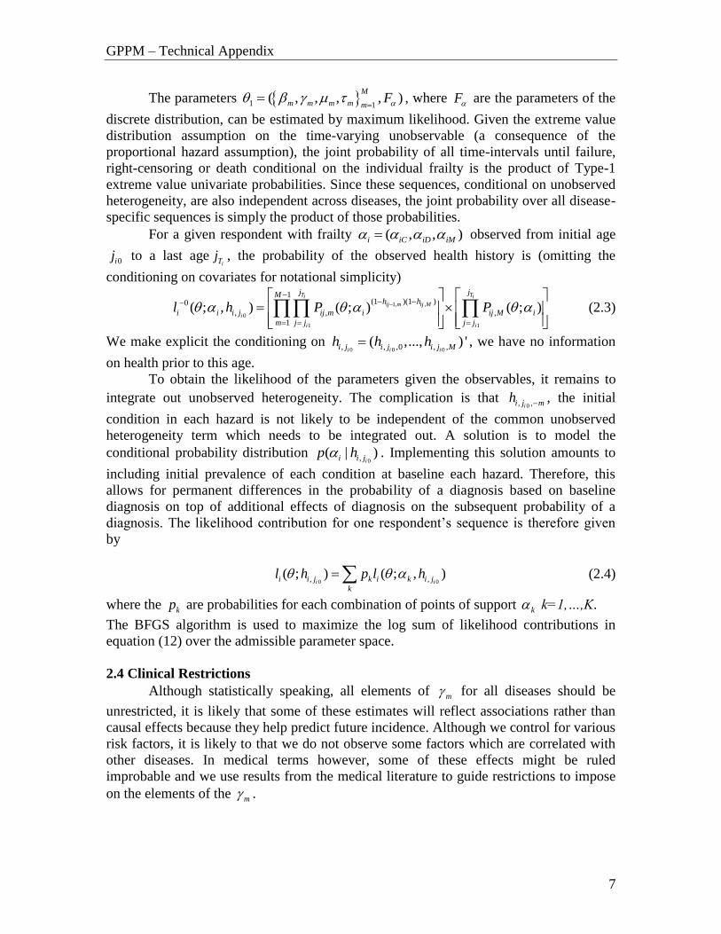
The parameters 1 1( , , , , )

M

m m m m mF

, where F are the parameters of the

discrete distribution, can be estimated by maximum likelihood. Given the extreme value

distribution assumption on the time-varying unobservable (a consequence of the

proportional hazard assumption), the joint probability of all time-intervals until failure,

right-censoring or death conditional on the individual frailty is the product of Type-1

extreme value univariate probabilities. Since these sequences, conditional on unobserved

heterogeneity, are also independent across diseases, the joint probability over all disease-

specific sequences is simply the product of those probabilities.

For a given respondent with frailty ( , , )i iC iD iM observed from initial age

0ij to a last ageiTj , the probability of the observed health history is (omitting the

conditioning on covariates for notational simplicity)

1, ,

0

1 1

1(1 )(1 )0

, , ,

1

( ; , ) ( ; ) ( ; )T Ti i

ij m ij M

i

i i

j jMh h

i i i j ij m i ij M i

m j j j j

l h P P

(2.3)

We make explicit the conditioning on 0 0 0, , ,0 , ,( ,..., ) '

i i ii j i j i j Mh h h , we have no information

on health prior to this age.

To obtain the likelihood of the parameters given the observables, it remains to

integrate out unobserved heterogeneity. The complication is that 0, ,ii j mh , the initial

condition in each hazard is not likely to be independent of the common unobserved

heterogeneity term which needs to be integrated out. A solution is to model the

conditional probability distribution 0,( | )

ii i jp h . Implementing this solution amounts to

including initial prevalence of each condition at baseline each hazard. Therefore, this

allows for permanent differences in the probability of a diagnosis based on baseline

diagnosis on top of additional effects of diagnosis on the subsequent probability of a

diagnosis. The likelihood contribution for one respondent’s sequence is therefore given

by

0 0, ,( ; ) ( ; , )

i ii i j k i k i j

k

l h p l h (2.4)

where the kp are probabilities for each combination of points of support k k=1,…,K.

The BFGS algorithm is used to maximize the log sum of likelihood contributions in

equation (12) over the admissible parameter space.

2.4 Clinical Restrictions

Although statistically speaking, all elements of m for all diseases should be

unrestricted, it is likely that some of these estimates will reflect associations rather than

causal effects because they help predict future incidence. Although we control for various

risk factors, it is likely to that we do not observe some factors which are correlated with

other diseases. In medical terms however, some of these effects might be ruled

improbable and we use results from the medical literature to guide restrictions to impose

on the elements of the m .


8

We use a set of clinical restrictions proposed by Goldman et al. (2005) based on

expert advice. It turns out that these restrictions are not rejected in a statistical sense one

we include initial conditions and unobserved frailty.

Table 2.1 Clinical Restrictions

prevalence t-1 heart

blood

pressure stroke

lung

disease diabetes cancer mental disability mortality

heart x x x x

blood pressure x x x x x

stroke x x x

lung disease x x x

diabetes x x x x x x

cancer x x x x

mental x x x

disability x x x

hazard at (t)

Notes: x denotes a parameter which is allowed to be estimated.

2.5 Descriptive Statistics and Estimation Results

For estimation, we construct an unbalanced panel from pooling all cohorts

together. We delete spells if important information is missing (such as the prevalence of

health conditions). Hence, in the final sample, a sequence can be terminated because of

death, unknown exit from the survey (or non-response to key outcomes), or finally

because of the end of the panel.

In each hazard, we include a set of baseline characteristics which capture the

major risk factors for each condition. We consider education, race & ethnicity, marital

status, gender and behaviors such as smoking and obesity. Finally, as discussed

previously, we also include a measure of the duration between interviews in month. The

average duration is close to 2 years. Table 2.2 gives descriptive statistics at first

interview.

Table 2.2 Baseline Characteristics in Estimation Sample

Characteristics (at first interview) N mean std. dev. min max

age in years 21302 64.1 11.2 50 103

less than high school 0.350 0.477 0 1

some college education 0.346 0.476 0 1

black 0.140 0.347 0 1

hispanic 0.068 0.251 0 1

married 0.703 0.457 0 1

male 0.431 0.495 0 1

ever smoked 0.591 0.492 0 1

obese (BMI>30) 0.210 0.407 0 1duration between interviews (in

months), averaged over all waves 23.4 2.8 1.8 30.9

Notes: All HRS Cohorts (HRS, AHEAD, CODA, War Babies)

Estimates of the hazard models are presented in Table 2.3. Estimates can be interpreted as

the effect on the log hazard. To judge the fit of the model we perform a goodness-of-fit


9

exercise. To do that, we re-estimate the model on a sub-sample and keep part of the

sample for evaluating the fit. We randomly select observations from the original HRS

cohort with probability 0.5 and simulate outcomes for this cohort starting from observed

1992 outcomes. Table 2.4 gives the observed frequencies as well as the predicted ones.

Predicted and observed frequencies are quite close to each other in 2002.


10

Table 2.3 Estimates with Heterogeneity and Clinical Restrictions

prevalence t-1 pe pe pe pe pe pe pe pe pe

heart -0.212 * 0.037 -0.160 * 0.599 **

blood pressure 0.033 0.042 0.169 * -0.115 0.426 **

stroke -0.172 0.240 * 0.864 **

lung disease -0.225 0.185 1.152 **

diabetes 0.062 0.346 ** 0.043 -0.422 ** -0.086 0.634 **

cancer -0.204 -0.141 0.222 ** 1.428 **

mental 0.336 ** 0.740 **

disability 0.199 ** 0.840 **

prevalence t=0

heart 0.076 0.483 ** 0.395 ** 0.190 ** 0.143 ** 0.272 ** 0.518 ** -0.220 **

blood pressure 0.358 ** 0.418 ** 0.046 0.578 ** 0.082 0.099 0.356 ** -0.277 **

stroke 0.030 0.238 ** -0.229 0.012 0.086 0.466 ** 0.425 ** -0.418 **

lung disease 0.511 ** 0.006 0.396 ** 0.014 0.301 ** 0.841 ** 0.627 ** -0.509 **

diabetes 0.540 ** 0.014 0.584 ** 0.014 -0.069 0.705 ** 0.711 ** 0.005

cancer 0.191 ** 0.050 0.244 0.259 ** -0.023 0.308 -0.128 -1.037 **

mental 0.335 ** 0.208 ** 0.422 ** 0.594 ** 0.171 * 0.012 0.512 ** -0.581 **

disability 0.330 ** 0.109 0.152 0.423 ** 0.127 0.057 0.478 ** -0.065

demographics

age <75 0.042 ** 0.021 ** 0.071 ** 0.019 ** 0.013 ** 0.044 ** -0.007 * 0.035 ** 0.030 **

age >75 0.038 ** -0.022 ** 0.055 ** -0.004 -0.044 ** -0.023 ** 0.038 ** 0.143 ** 0.112 **

black -0.268 ** 0.336 ** 0.153 * -0.363 ** 0.210 ** -0.092 -0.225 ** 0.447 ** 0.244 **

hispanic -0.441 ** 0.095 -0.199 -0.582 ** 0.420 ** -0.370 ** 0.194 ** 0.424 ** -0.073

male 0.336 ** -0.109 ** 0.063 -0.146 ** 0.364 ** 0.366 ** -0.458 ** -0.195 ** 0.420 **

ever smoked 0.176 ** -0.009 0.255 ** 1.040 ** 0.102 * 0.257 ** 0.187 ** 0.210 ** 0.344 **

obese (BMI>30) 0.196 ** 0.350 ** 0.106 0.059 1.065 ** 0.027 -0.032 0.552 ** -0.273 **

high school -0.169 ** -0.091 * -0.137 * -0.356 ** -0.274 ** -0.024 -0.334 ** -0.430 ** -0.029

college -0.191 ** -0.146 ** -0.252 ** -0.581 ** -0.312 ** 0.088 -0.461 ** -0.586 ** -0.168 **

log(time since l.w.) 0.996 ** 1.224 ** 1.242 ** 1.015 ** 1.296 ** 1.063 ** 1.102 ** 0.614 ** 6.547 **

constant -6.573 ** -6.121 ** -8.592 ** -7.164 ** -8.016 ** -7.859 ** -6.121 ** -4.433 ** -26.079 **

point 1 0 0 0 0 0 0 0 0 0

point 2 -1.353 ** -1.353 ** -1.353 ** -1.353 ** -1.353 ** -1.353 ** -1.353 ** -2.164 ** -2.176 **

Loading Factor 1 0.625 ** 1.637 ** 1.085 ** 0.678 ** 0.244 ** 1.308 ** 1 1

Probability estimates

point p(1,1,1) p(1,1,2) p(1,2,1) p(1,2,2) p(2,1,1) p(2,1,2) p(2,2,1) p(2,2,2)

Probability 0.193 ** 0.082 ** 0 0.024 ** 0.085 ** 0 0.530 ** 0.087 **

loglike/N -3.632

MortalityDiabetes Cancer Mental DisabilityHeart disease Blood pressure Stroke Lung disease


11

Table 2.4 Goodness-of-Fit

Prevalence Rate (Independent Draws)

year data sim data sim data sim data sim

1992 0.117 0.120 0.347 0.344 0.027 0.027 0.061 0.062

1994 0.138 0.147 0.376 0.393 0.030 0.037 0.074 0.074

1996 0.157 0.172 0.401 0.437 0.039 0.046 0.078 0.087

1998 0.176 0.196 0.435 0.478 0.047 0.055 0.088 0.097

2000 0.199 0.218 0.480 0.516 0.056 0.063 0.093 0.106

2002 0.236 0.241 0.527 0.551 0.064 0.072 0.109 0.113

# cond. 825 853 1843 1949 224 254 380 399

year data sim data sim data sim data sim

1992 0.104 0.108 0.058 0.058 0.053 0.056 0.072 0.072

1994 0.121 0.130 0.065 0.076 0.094 0.116 0.090 0.095

1996 0.137 0.150 0.078 0.093 0.160 0.164 0.104 0.115

1998 0.151 0.169 0.093 0.111 0.197 0.205 0.118 0.133

2000 0.169 0.185 0.107 0.125 0.224 0.237 0.131 0.148

2002 0.199 0.201 0.125 0.141 0.248 0.264 0.154 0.160

# cond. 695 711 436 500 867 934 540 566

data sim data sim data sim data sim

year

1992 0.475 0.476 0.317 0.311 0.136 0.138 0.072 0.075

1994 0.422 0.390 0.328 0.329 0.149 0.166 0.101 0.115

1996 0.371 0.323 0.326 0.333 0.168 0.191 0.134 0.153

1998 0.324 0.270 0.321 0.326 0.191 0.211 0.163 0.192

2000 0.279 0.230 0.312 0.315 0.215 0.229 0.194 0.226

2002 0.231 0.199 0.295 0.299 0.235 0.240 0.238 0.263

Incidence Rate

Goodness-of-Fit test

year data sim Prevalence rates 4.05 0.774

1992 0.000 0.000 (dF = 7)

1994 0.014 0.009

1996 0.014 0.012 Np 3539

1998 0.016 0.014

2000 0.019 0.017 Nu 3500

2002 0.019 0.020

Notes: Simulation for HRS 1992 subsample (N=4131)

heart pressure stroke lung

mental

mortality

diabetes cancer disability

1 cond 2 cond 3 cond.+no conditions


12

2.5 Adjusting the Model to European Transitions

In continental Europe, we only have access to cross-sectional data on responses of the

type: has the doctor ever told you. Hence, the age distribution is informative about

transition rates to the extent that we make assumptions about features of the model which

we are willing to assume is similar across the Atlantic. We make those conditions more

precise below.

We split the 2004 cross section in two groups based on age. Denote by subscript 0 the

first younger group and 1 the second older group. Data takes the form of a set of

conditions y and characteristics x for the two samples in year t=2004. We have

00 0 1,...,{ , }i i i ny x and 11 1 1,...,{ , }i i i ny x in 2004. For convenience also denote by ( , )z y x . The

data generating process is assumed given by

1 0( | ; )t tF z z (2.5)

where 0 represents the true value of the parameter vector characterizing this DGP. This

is essentially our transition model. The dimension of this parameter vector is K .

Indirect Inference

One key assumption allows to make inference based on simulated outcomes is that data

from both groups are generated from the same DGP (Eq 1).

Under this assumption, it is possible, for a given value of to simulate outcomes of

group 0 when they will reach the age of group 1. If the distribution of simulated

outcomes or any other moment or auxiliary parameter comes close to that of outcomes of

group 1, then it must be that 0 . The general class of such estimators is called

Simulated Minimum Distance (SMD) (Hall and Rust, 1999) and includes as special cases

the method of simulated moments (Pakes and Pollard, 1989) and Indirect Inference

(Gourieroux, Monfort and Renault, 1993).

For a given simulation j , denote simulated outcomes by 00 1,...,{ ( , )}ij i i nz z . Assume an

auxiliary model that yields parameters 0( , )z (Px1) when estimated on this simulated

data.

Under assumption 1 and general regularity conditions,

0 0 1( ( , )) ( )jE z z (2.6)

where 1( )z are the auxiliary parameters estimated from group 1. Based on J

simulations, a consistent estimator of the left hand side of (2) for a trial value of is

given by


13

1

0 01,..,( , ) ( , )jj Jz J z

(2.7)

Hence, 0 can be consistently estimated by

arg min ( , ) ' ( , )I Pg z g z (2.8)

where 0 1( , ) ( , ) ( )g z z z and P is some positive definite matrix of dimension P.

If P = K, then the model is just identified and I is such that

( , ) 0Ig z (2.9)

Auxiliary Model

An important condition for local identification is that 0( , )g z be of full rank. Hence

the choice of an auxiliary model is important. Because some features of the model are

difficult to identify from the cross-sectional information in SHARE, we decide to only re-

estimate a subset of the parameters. In particular, we allow the intercept of the hazard to

be adjusted and fix other parameters to their U.S. value.

We choose the following auxiliary model for the prevalence of each condition m,

, 0, ,a m m a mp (2.10)

The parameters of such model can be estimated consistently by OLS. For all health

conditions such model can be estimated from the SHARE data using appropriate weights.

However, for mortality this is not possible because SHARE is a cross-section. We use

each country’s life-table mortality profiles to estimate the auxiliary parameters. We

weight those by population to get aggregate numbers. These are then compared to the

simulated mortality profile in SHARE.

These parameters bear close relationship with the constant and age profile of each

condition’s hazard. Since the number of structural parameters is equal to the number of

auxiliary parameters, the model is just identified. Hence, there is no need to choose a

weighting matrix. If estimation reveals that the minimum is not zero, this means the

model is misspecified (Alvarez et al., 2001).

Estimation

Because the criterion is effectively a step function (outcomes are discrete), numerical

optimization using standard gradient method becomes difficult without having to increase

prohibitively the number of replications. Instead we use the Nelder-Mead Simplex

algorithm which is not based on gradient methods and hence can optimize non-smooth


14

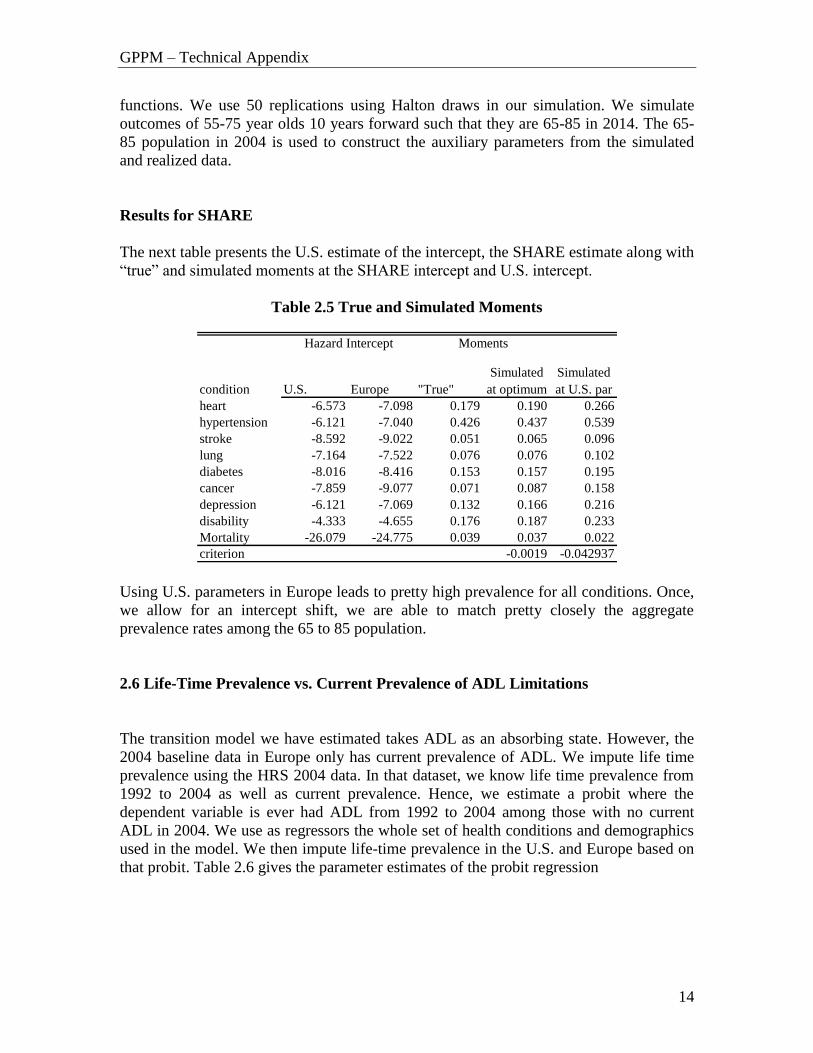
functions. We use 50 replications using Halton draws in our simulation. We simulate

outcomes of 55-75 year olds 10 years forward such that they are 65-85 in 2014. The 65-

85 population in 2004 is used to construct the auxiliary parameters from the simulated

and realized data.

Results for SHARE

The next table presents the U.S. estimate of the intercept, the SHARE estimate along with

“true” and simulated moments at the SHARE intercept and U.S. intercept.

Table 2.5 True and Simulated Moments

condition U.S. Europe "True"

Simulated

at optimum

Simulated

at U.S. par

heart -6.573 -7.098 0.179 0.190 0.266

hypertension -6.121 -7.040 0.426 0.437 0.539

stroke -8.592 -9.022 0.051 0.065 0.096

lung -7.164 -7.522 0.076 0.076 0.102

diabetes -8.016 -8.416 0.153 0.157 0.195

cancer -7.859 -9.077 0.071 0.087 0.158

depression -6.121 -7.069 0.132 0.166 0.216

disability -4.333 -4.655 0.176 0.187 0.233

Mortality -26.079 -24.775 0.039 0.037 0.022

criterion -0.0019 -0.042937

MomentsHazard Intercept

Using U.S. parameters in Europe leads to pretty high prevalence for all conditions. Once,

we allow for an intercept shift, we are able to match pretty closely the aggregate

prevalence rates among the 65 to 85 population.

2.6 Life-Time Prevalence vs. Current Prevalence of ADL Limitations

The transition model we have estimated takes ADL as an absorbing state. However, the

2004 baseline data in Europe only has current prevalence of ADL. We impute life time

prevalence using the HRS 2004 data. In that dataset, we know life time prevalence from

1992 to 2004 as well as current prevalence. Hence, we estimate a probit where the

dependent variable is ever had ADL from 1992 to 2004 among those with no current

ADL in 2004. We use as regressors the whole set of health conditions and demographics

used in the model. We then impute life-time prevalence in the U.S. and Europe based on

that probit. Table 2.6 gives the parameter estimates of the probit regression


15

Table 2.6 Probit Regression Results for Imputation of Life-Time prevalence of ADL

Limitations

par std t p-val

heart 0.244 0.035 6.92 0

hypertension 0.063 0.034 1.88 0.06

stroke 0.293 0.052 5.58 0

lung disease 0.317 0.048 6.59 0

diabetes 0.069 0.040 1.72 0.085

cancer 0.032 0.043 0.75 0.455

mental 0.503 0.040 12.5 0

age 0.014 0.002 7.61 0

black 0.341 0.045 7.51 0

hispanic 0.290 0.059 4.89 0

male -0.105 0.033 -3.16 0.002

ever smoked 0.054 0.033 1.64 0.1

high school -0.195 0.041 -4.81 0

college -0.340 0.042 -8.04 0

obese 0.240 0.036 6.65 0

intercept -2.338 0.145 -16.15 0

Notes: probit coefficients from HRS 2004 sample of those

currently not reporting any ADL where dependent variabie is

1992-2004 prevalence of ADL


16

3. Calculating the Health Effect of new Drugs

Prior to the introduction of a new drug, it is useful to think of the population as

divided into three subgroups: Those undiagnosed for a particular health condition, those

diagnosed with a condition and treated with an existing drug, and finally those who are

diagnosed but untreated. We can think of the new drug as one that potentially reduces

mortality risk or the risk of being diagnosed with another health condition (e.g. a new

drug that treats hypertension may reduce the risk of being diagnosed with heart disease).

Figure 3.1 illustrates how each sub-population benefits from a new drug. The treated

group may benefit because new drugs are potentially more effective than existing

treatments. We will call this the “clinical effect.” A fraction of the previously untreated

group may however gain access to this treatment. This group will thus experience the full

health effect of a new drug (relative to no treatment). We will refer to this as the “access

effect”. Finally, the remaining untreated individuals do not gain from the introduction of

the drug.3

Figure 3.1 Effect of a New Drug

In such a population, the average effect of a new drug will be a weighted average of

the clinical and access effect. To see this, denote by ( 0 1, ) the fraction of diagnosed

individuals who are untreated before and after the introduction of the new drug,

respectively, and define 0 1 . Denote P as the probability of being diagnosed

3 This abstracts from any effect on diagnosis and thus provides a lower bound on the total effect of new

drugs.

Population diagnosed Population undiagnosed: No Effect

Treated: Effect Relative to Existing

Treatment

Untreated

Untreated with Access:

Effect relative to

“Placebo”

Untreated without

Access:

No Effect


17

with a new condition or death, and / , /EXISTING NEW EXISTING PLACEBO NEW PLACEBORR P P RR P P

to be the relative risk for those replacing existing therapy with the new drug, and those

replacing no therapy with the new drug, respectively. Note that the latter corresponds to

the risk given by the new drug, divided by the risk given by placebo treatment. As such,

the annual relative risk for the diagnosed population following the introduction of a new

drug (relative to the pre-existing situation) is given by

1 0[ ] [(1 ) ]PLACEBO U EXISTING TRR P RR PRR

P

(3.1)

where UP is the average probability of contracting another condition or death among the

untreated, TP is that average probability among the treated and 0 0(1 )U TP P P is

the average probability in the diagnosed population prior to the introduction of the drug.

The first term of the numerator on the right hand side of equation (1) represents

the total effect on the untreated, including the access effect, while the second term

represents the clinical effect on those that were already treated prior to the new drug

introduction. These two effects are weighted by the pre-introduction mean probability of

being diagnosed with the new condition or death in the untreated and treated group

separately.

For example, suppose a new drug is introduced which potentially reduces mortality

for patients diagnosed with cancer. Compared with existing treatment, this drug is 25%

more effective. Compared with no treatment, however, it leads to a 50% decrease in

mortality risk. Now, suppose 50% of patients diagnosed with Cancer take the existing

treatment and that both treated and untreated patient face a survival probability of 75%.

Finally assume the introduction of the new drug means that 25% more patients are

treated. This leads a 25% reduction in untreated patients. Hence, 25% of the diagnosed

population derives no benefit, 25% enjoy a 50% decrease in mortality risk because they

move from no treatment to the new therapy, and the remaining 50% of the population

enjoy the 25% improvement over existing treatment. The average relative risk is then

0.25+0.25*0.5 + 0.5*0.75 = 0.75 for the diagnosed population.4 Note that ignoring the

access effect amounts to imposing 0 . In this case, only the treated will benefit from

the new drug. For many diseases, this access effect can be important, particularly when

access is relatively low and existing treatments are not easily accessible. The same

calculations can be performed for other risks such as the risk of being diagnosed for

another health condition.

In Section 3.1, we provide methodologies for estimating each of the components of

equation 1. Section 3.1 is devoted to the construction of a list of drugs for each of the

4 This method accounts for differences in disease severity between untreated and treated individuals.

However, note that our approach presumes that the effects of drugs can be appropriately captured by

computing the average reduction in risk. An alternative would be to explicitly assign different reductions

in risk to different people — e.g., those with different disease severity levels. While the latter approach

would be more general, data limitations preclude its implementation: we do not have a panel of data on

treatment status, which makes it ultimately impossible for us to separately model disease dynamics for the

treated and untreated population.


18

conditions we consider. For these drugs, the relative risks (RR) are then taken from

clinical trials in section 3.2. Section 3.3 is devoted to the estimation of the access effect

( ) from claims data. In section 3.4, we calculate the remaining parameters ( 0 , ,U TP P )

from the Health and Retirement Study.

3.2 Estimation

For each of the health condition in the transition model, one could in principle

consider the whole universe of new drugs and calculate an average effect for each of

them. This is likely to be a difficult task. However, breakthrough drugs are the most

likely to have clinical effects, and have been in general the most studied and reviewed.

This makes the estimated clinical benefits more reliable. For each of our diseases,

therefore, we survey the clinical effects for the top 5 selling (or “blockbuster”) drugs in

that disease group, and assume conservatively that all other drugs outside the top 5 have

no therapeutic benefits. Therefore, we estimate the effects of drugs in two parts:

calculate the probability that a new drug will be a “top-seller,” and apply the expected

therapeutic benefit of a top-selling drug.

3.2.1 List of New Blockbuster Drugs

We construct a list of new drugs from INGENIX, a large, nationwide, longitudinal

claims-based database (1997-2004).5 This data set has drug expenditure information from

insurance plan enrollees. We use expenditures as a proxy to identify blockbuster drugs.

Health conditions in INGENIX are provided at the patient level, which makes it difficult

to match drugs to health conditions because patients can take medication for multiple

diseases at the same time. For example, it is unclear whether a drug used by a heart

disease patient with hypertension is used to treat the heart condition or hypertension.

Mapping drugs to Redbook drug class and then to health conditions appears to be a

superior strategy. Hence, we first group drugs by class and then assign each class to at

least one particular health condition, based on expert opinion and an extensive web

search.6 The result of this class-health condition match is presented in Appendix A.

We rank drugs for each health condition according to revenues in the 2nd year

following introduction.7 We consider new chemical entities (NCEs) as well as

reformulation and recombination drugs, but exclude generics. We define the top 5 drugs

for each health condition as “Blockbuster drugs”. The name of the drug, Redbook drug

class, generic name, and the introduction date are presented in Appendix B.

3.2.2 Calculating Effects on Health

5 Due to the time range of INGENIX dataset, the list was limited to drugs approved by FDA from 1995 to

2002. 6 A log of the search results is available from the authors upon request. 7 We deflate expenditures using the general CPI.


19

For each of the blockbuster drugs, we survey the medical literature for clinical trials.

When the trials do not provide an estimate for the health condition we are interested in,

we assume the drug has no effect. Hence, these estimates can be seen as conservative. We

do the same when the estimate is not statistically significant. When more than one

estimate is available, we use the mean of the effects found.

We searched for the impacts of blockbuster drugs on mortality, and on the incidence

of all 6 other health conditions under consideration. However, we follow Goldman et al.

(2005) in ruling out some causal links, based on expert opinion. For example, we assume

that there is a causal link between hypertension and diabetes, but not from hypertension

to cancer. We do not investigate the effect of new drugs on recovery or cure rates. Table

1 summarizes results from the survey of the literature for those effects. Appendix C gives

detail on the calculation of each estimate. These calculations provide the estimates of

EXISTINGRR and PLACEBORR in equation 1.


20

Table 3.1 Summary of Clinical Effects Found in Medical Literature

Condition treated RR(P) RR(E) RR(P) RR(E) RR(P) RR(E) RR(P) RR(E) RR(P) RR(E) RR(P) RR(E) RR(P) RR(E) RR(P) RR(E)

heart diseae 0.475 1 1 1 1 1

hypertension 0.643 1 0.729 1 1 1 1 1

stroke 1 1 1 1

lung disease 1 1 1 0.796

diabetes 0.690 1 1 1 0.533 1 1 1 0.52 1

cancer 1 1 1 1 0.837 0.728

depression 1 1

Notes: See Appendix C for details on the calculations. This matrix assumes a set of causal clinical mechanisms described in Goldman et al. (2004) Empty cell

mean that no elevated risk of a new condition is assumed due to the condition treated(no causal effect).

Health Outcome (Relative Risk RR(): New Drug/Control, Control is P=Placebo, E=Existing Treatment)

Heart disease Hypertension Stroke Lung Disease Diabetes Cancer Depression Mortality


21

3.2.3 Access Effect

To calculate the access effect, we need to construct an estimate of which is

the decrease in the fraction of untreated individuals following the introduction of a new

drug. We estimate this effect using prescription data from the IMS data.8 By merging the

drug consumption data with data on the introduction date of new drugs (from Appendix

B), we get a panel data set of the number of prescriptions consumed monthly for each

class before and after the introduction of the top 5 drugs (from 1997.1 to 2004.12).9 Our

strategy is to compute the effect of a launch on prescriptions relative to the trend in

prescriptions for a specific class. The statistical model that implements this strategy

explains the logarithm of monthly prescriptions in a class c as

0 3 3 6 6 12 12

, 0 , 3 , 6 , 12 , ,log( ) ( )c t c c c t c t c t c t c tC g t L L L L (2)

c are class fixed effects, ( )cg t is some class specific function of calendar time. The

variables ,

k

c tL are indicator functions that take value 1 when a new blockbuster drug has

been on the market for k months. Finally is some unobserved disturbance with zero

mean. We specify linear class-specific time trends: ( )c cg t t , which was not rejected

against a more flexible specification. Hence the total effect of a new drug on

prescriptions after 12 months is given by 12 . We also include interaction terms to

differentiate if the new drug is a reformulation or a new chemical entity (NCE). This

interaction measures the effect of reformulation drug relative to a new NCE, i.e. a

negative coefficient indicates that the effect of reformulation is smaller than the effect of

a NCE. Table 2 presents estimation results.

8 http://www.imshealth.com 9 We use the USC-5 classification which results in 22 classes for the purpose of estimation.


22

Table 3.2 Access Effect Regression Results

Coefficient P-Value

Launched 0~3

Months 0.064 0.543

(Launched 0~3

months)*Reformul

ation 0.001 0.993

Launched 3~6

Months 0.241 0.076

(Launched 3~6

months)*Reformul

ation -0.272 0.060

R-Square: 0.973

Launched 6~12

Months 0.301 0.033

(Launched 6~12

months)*Reformul -0.262 0.064

Launched >=12 0.258 0.035(Launched >=12

months)*Reformul

ation -0.245 0.049

Number of

observations:

2711

Time period:

Jan 1997~Dec

2004

Notes: OLS regression of log(number of prescriptions).

Standard errors allow for clustering at the USC-5 class level.

New chemical entities tend to have a relatively strong effect on the number of

prescriptions after 3 months. After one year, there is a 32% increase in the number of

prescriptions. This estimate is statistically significant at the 10% level. On the other hand,

the effect for reformulations is small and negligible. Figure 2 presents the estimates of the

effect separately for NCEs and reformulations. A statistical test confirms that it is very

unlikely that prescriptions increase following the introduction of a reformulation.10 The

effect for NCEs is used to compute the assuming that this effect comes from more

individuals being treated rather than more prescriptions awarded by existing patients.

10 In principle, it would be possible to isolate a separate effect for each health conditions since there are

generally more than one drug class that treats a condition. The problem is that for some conditions (stroke,

diabetes and depression) few classes are used hence leading to identification problems. Estimates from such

specifications did not yield differences that were statistically different from each other.


23

Figure 3.2 Access Effect

Notes: Based on Estimation Results from Table 2. Regression of monthly log(number

of prescriptions) on launch of new chemical entities and reformulations.

-5.0%

0.0%

5.0%

10.0%

15.0%

20.0%

25.0%

30.0%

35.0%

0~3 3~6 6~12 >=12

Months After Launch

% I

ncr

ease

in

pre

scri

ptio

ns

New Chemical

EntitiesReformulations

3.2.4 Access and Incidence Rates by Conditions

Three more estimates are needed to compute average relative risks from equation

1. First, we need to know, for each condition, the fraction of diagnosed individuals not

taking existing drugs ( 0 ). Second, we need estimates of the incidence rates for those

treated ( TP ) and untreated ( UP ). We use the Health and Retirement Study (HRS) for that

purpose. The HRS is a nationally representative longitudinal study of the age 50+

population. It asks about lifetime prevalence of the seven conditions we use as well as the

consumption of drugs for those diagnosed with these conditions. It also tracks mortality.

Mortality rates from the HRS follow closely figures from life-tables (Adams et al.,

2003).11 Most of the differences are attributable to the fact that HRS samples the non-

institutionalized population.

To construct estimates of the transition rates (P), we use hazard models estimated

on the 1992-2002 waves of the HRS. The hazard models include baseline demographics,

prevalence indicators at the previous wave, risk behaviors, and age. Table 3 gives the

lifetime prevalence in 2004 of various conditions, the fraction untreated among the

diagnosed population and predicted transition rates based on hazard models.

11 The HRS conducts exit interviews with relatives for deceased respondents. If a respondent’s status in one

wave is unknown, an interview is attempted in following waves until it can be established.


24

Table 3.3 HRS Disease Prevalence, Drug Usage, and Predicted Incidence Rate

condition treated prevalence untreated treated untreated treated untreated treated untreated treated untreated treated

heart disease 0.253 0.338 0.173 0.026 0.030 0.028 0.031 0.037 0.047

hypertension 0.546 0.110 0.110 0.048 0.050 0.022 0.023 0.024 0.024 0.026 0.027

stroke 0.080 0.632 0.096 0.039 0.040 0.063 0.069

lung disease 0.102 0.467 0.140 0.040 0.047 0.047 0.053

diabetes 0.176 0.183 0.183 0.068 0.071 0.074 0.081 0.032 0.032 0.029 0.030 0.041 0.040

cancer 0.141 0.772 0.060 0.022 0.022 0.026 0.021 0.040 0.037

mental 0.165 0.426 0.150 0.032 0.029

Notes: Calculations from HRS 2004 data. Sample weights used.

fraction

untreated

before

introduction

Mortality

reduction in

fraction

untreated

Predicted Incidence Rate Prior to Introduction For

Hypertension StrokeHeart disease Depression


25

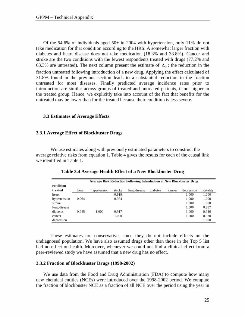
Of the 54.6% of individuals aged 50+ in 2004 with hypertension, only 11% do not

take medication for that condition according to the HRS. A somewhat larger fraction with

diabetes and heart disease does not take medication (18.3% and 33.8%). Cancer and

stroke are the two conditions with the fewest respondents treated with drugs (77.2% and

63.3% are untreated). The next column present the estimate of : the reduction in the

fraction untreated following introduction of a new drug. Applying the effect calculated of

31.8% found in the previous section leads to a substantial reduction in the fraction

untreated for most diseases. Finally predicted average incidence rates prior to

introduction are similar across groups of treated and untreated patients, if not higher in

the treated group. Hence, we explicitly take into account of the fact that benefits for the

untreated may be lower than for the treated because their condition is less severe.

3.3 Estimates of Average Effects

3.3.1 Average Effect of Blockbuster Drugs

We use estimates along with previously estimated parameters to construct the

average relative risks from equation 1. Table 4 gives the results for each of the causal link

we identified in Table 1.

Table 3.4 Average Health Effect of a New Blockbuster Drug

condition

treated heart hypertension stroke lung disease diabetes cancer depression mortality

heart 0.919 1.000 1.000

hypertension 0.964 0.974 1.000 1.000

stroke 1.000 1.000

lung disease 1.000 0.887

diabetes 0.945 1.000 0.917 1.000 0.910

cancer 1.000 1.000 0.930

depression 1.000

Average Risk Reduction Following Introduction of New Blockbuster Drug

These estimates are conservative, since they do not include effects on the

undiagnosed population. We have also assumed drugs other than those in the Top 5 list

had no effect on health. Moreover, whenever we could not find a clinical effect from a

peer-reviewed study we have assumed that a new drug has no effect.

3.3.2 Fraction of Blockbuster Drugs (1998-2002)

We use data from the Food and Drug Administration (FDA) to compute how many

new chemical entities (NCEs) were introduced over the 1998-2002 period. We compute

the fraction of blockbuster NCE as a fraction of all NCE over the period using the year in


26

which they were approved by the FDA. We map each approved drug to health

condition(s) by using the indications listed by the FDA in its annual report. We exclude

reformulations and recombination drugs for two reasons. First, indications are only given

for NCEs so that we cannot do the mapping for reformulation and recombination drugs.

Second, reformulation and recombination drugs are not likely to have clinical effects over

existing treatments because they simply recombine or reformulate existing treatments.

This leaves the possibility that they have an access effect. But we could not find any

access effect for those drugs in section 3.3. Hence, we can ignore such drugs in our

calculations. Table 5 presents the results for the fraction of blockbuster NCEs from

1998-2002. The fraction of new blockbuster drugs is quite different across diseases

ranging from 10% for hypertension to 67% for stroke (only one new NCE for depression

is approved by the FDA over the period and it is a blockbuster drug).


27

Table 3.5 Probability of a New Blockbuster Drug for Each Health Condition, 1998-2002

New drugs

total top total top total top total top total top total top total top

1998 3 0 3 0 0 0 1 0 0 0 3 1 1 1

1999 1 0 1 0 0 0 2 0 2 2 5 2 0 0

2000 2 1 1 0 2 1 1 1 3 0 4 0 0 0

2001 2 0 2 1 1 1 2 0 0 0 2 1 0 0

2002 2 1 3 1 0 0 0 0 0 0 2 0 0 0

Total 10 2 10 2 3 2 6 1 5 2 16 4 1 1

Average 2 0.4 2 0.4 0.6 0.4 1.2 0.2 1 0.4 3.2 0.8 0.2 0.2

Fraction top 0.20 0.20 0.67 0.17 0.40 0.25 1.00

Diabetes Cancer Depression

Notes: Information on new chemical entities taken from the FDA websites. The FDA lists indications for each drug which were then mapped to our set of conditions. The top-selling drugs are identified in

Appendix A according to revenues, two years after introduction according to the INGENIX database.

Heart Hypertension Stroke Lung Disease


28

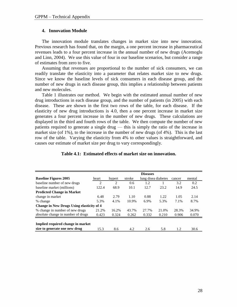
4. Innovation Module

The innovation module translates changes in market size into new innovation.

Previous research has found that, on the margin, a one percent increase in pharmaceutical

revenues leads to a four percent increase in the annual number of new drugs (Acemoglu

and Linn, 2004). We use this value of four in our baseline scenarios, but consider a range

of estimates from zero to five.

Assuming that revenues are proportional to the number of sick consumers, we can

readily translate the elasticity into a parameter that relates market size to new drugs.

Since we know the baseline levels of sick consumers in each disease group, and the

number of new drugs in each disease group, this implies a relationship between patients

and new molecules.

Table 1 illustrates our method. We begin with the estimated annual number of new

drug introductions in each disease group, and the number of patients (in 2005) with each

disease. These are shown in the first two rows of the table, for each disease. If the

elasticity of new drug introductions is 4.0, then a one percent increase in market size

generates a four percent increase in the number of new drugs. These calculations are

displayed in the third and fourth rows of the table. We then compute the number of new

patients required to generate a single drug — this is simply the ratio of the increase in

market size (of 1%), to the increase in the number of new drugs (of 4%). This is the last

row of the table. Varying the elasticity from 4% to other values is straightforward, and

causes our estimate of market size per drug to vary correspondingly.

Table 4.1: Estimated effects of market size on innovation.

Baseline Figures 2005 heart hypert stroke lung diseasediabetes cancer mental

baseline number of new drugs 2 2 0.6 1.2 1 3.2 0.2

baseline market (millions) 122.4 68.9 10.1 12.7 23.2 14.9 24.5

Predicted Change in Market

change in market 6.48 2.79 1.10 0.88 1.22 1.05 2.14

% change 5.3% 4.1% 10.9% 6.9% 5.3% 7.1% 8.7%

Change in New Drugs Using elasticity of 4

% change in number of new drugs 21.2% 16.2% 43.7% 27.7% 21.0% 28.3% 34.9%absolute change in number of drugs 0.423 0.324 0.262 0.332 0.210 0.906 0.070

Implied required change in market

size to generate one new drug 15.3 8.6 4.2 2.6 5.8 1.2 30.6

Diseases


29

This method provides us with the number of new drugs for each disease. The probability

of a top-seller in each disease group is then applied to these results to generate the

number of new top-sellers each year. The realization is drawn from a binomial trial for

each new drug. The realization of ,m td , the number of new top-seller drugs, is then

applied to health transition probabilities. For example, the mortality probability of

individual i, ,

T

m itP ,after applying the clinical effect mRR is

,

, , 1 ,[1 ]m td

T Umm it m it m itP h RR P . (4.2)

We assume there is 10 year lag between the decision to start research on a new drug and

the time it arrives on the market. Hence, new drugs at time t depend on changes in market

size at t-10.

5. Costs and Benefits

5.1 Value of Remaining Life-Years

Denote by ,a tn the number of people of age a alive in alive in year t. In any given

year, the value of discounted life-years ahead can be calculated from the simulation.

Using a discount rate and a value of a statistical life year v , this is given by

( )

, ( ),

T s t

a t a s t ss tN v n

(5.1)

We use a discount rate of 3% to discount benefits as well as expenditures.

5.2 Medical and Drug Expenditures

Because the HRS does not have accurate information on total medical expenditures and

total drug expenditures, we use the Medical Expenditure Panel Study (MEPS) to

construct cost regressions. We regress these expenditure on the same demographics we

have in the model as well as age and health condition indicators. Few differences in the

definition of variables are observed. We use the sample of age 50+ individuals in MEPS.

The regressions are performed separately for male and female as well as for each type of

expenditure (drug and medical). The regression takes the form:

,i t a it it x it h ity a x h (5.2)

Medicare Current Beneficiary Survey (MCBS) provides a better medical cost expenditure

estimation for elderly( age 65+). We mapped the MEPS regression results to MCBS

average values for the elderly, by adjusting the constant and age variable coefficients.

Table 5.1 gives the final results after MEPS regression and mapping MEPS to MCBS:.


30

Table 5.1 Cost Regression Results for Female and Males aged 50+

Drug Expenditure

(annual $) coeff s.e. coeff s.e.

heart 670.78 50.72 3212.32 232.74

hypertension 593.41 42.24 392.94 193.84

stroke 545.88 81.75 2665.75 375.12

lung 572.19 107.04 2565.87 491.17

diabetes 1075.22 56.95 2150.18 261.34

cancer 477.58 84.79 4268.14 389.09

mental 967.90 49.27 1024.93 226.07

disability 935.43 89.92 8150.39 412.63

age<68 3.17 5.02 37.78 23.05

age>68 -4.00 5.29 145.78 24.29

age 68 -36.11 79.19 1801.86 363.37

black -151.62 57.44 -481.06 263.57

hispanic -229.83 62.99 -286.53 289.05

smoke ever 49.72 39.99 312.61 183.52

obese 150.00 44.10 -52.18 202.39

l.t. highschool -26.23 44.53 64.35 204.33

college -90.11 61.90 479.82 284.05

constant 835.44 95.50 2735.13 438.25

R-square 0.21 0.32

Medical expenditure

annual ($) coeff s.e. coeff s.e.

heart 626.43 41.76 3976.53 336.93

hypertension 581.76 35.41 880.40 285.68

stroke 477.00 69.07 2453.71 557.21

lung 702.77 77.02 1885.78 621.37

diabetes 986.95 47.87 1324.49 386.23

cancer 158.61 73.65 5746.56 594.14

mental 762.65 56.21 2059.72 453.50

disability 936.47 97.48 11134.07 786.39

age<68 25.87 4.08 41.28 32.93

age>68 12.20 4.97 114.46 40.13

age 68 -1.11 67.43 573.70 544.02

black 33.05 51.20 -477.30 413.03

hispanic -99.43 54.81 -106.81 442.16

smoke ever 56.98 35.08 448.36 283.02

obese 208.62 39.61 406.22 319.53

l.t. highschool 40.98 40.16 1031.26 323.96

college 62.65 46.98 1473.59 379.02

constant 599.46 82.36 1903.32 664.44

Sample size 9141 6205

R-square 0.13 0.12

Notes: OLS regression results using robust standard errors on MEPS data

female male

female male

For Europe, we adjust costs using the ratio of expenditure per capita across countries.

These figures are given by the OECD. Table 5.2 provides detail on the calculations


31

Table 5.2 Total Expenditure on Pharmaceutical and Non-Pharmaceutical Services

by Country

Non-pharma pharmaNon-pharma pharma

Denmark 2610 271 0.49 0.36

France 2562 597 0.48 0.80

Germany 2566 439 0.48 0.58

Greece 1786 376 0.33 0.50

Italy 1880 512 0.35 0.68

Netherlands 2691 350 0.50 0.47

Spain 1617 477 0.30 0.64

Sweden 2478 347 0.46 0.46

U.S. 5351 751 1.00 1.00

Source:

Ratio Country vs. US

OECD Health Data 2005

Total expenditure per

capita $USD 2004 PPP

6. Stochastic Simulation and Weighting

The horizon for each simulation is 2005 to 2150 by which time all 2060 new entrants are

all dead. We start the simulation with the HRS and SHARE 2004 samples. We adjust

weights so that they match 2004 population counts provided by the United Nations’

Population Program. We do this by age in order to smooth out bumps in the age

distribution. Each year, the population of age 55 respondents in 2004 is added back

adjusting their weights for projected demographic trends. Table 6.1 presents forecasted

growth rates. By using the age 55 2004 cohort repeatedly and only adjusting for growth,

we do not take into account of composition effects due to different growth rates across

different segment of the population (say obese population)

Table 6.1 Population Age 55-59 Growth Rate Projections from United Nations

year SHARE US

2010 0.009 0.028

2015 0.014 0.021

2020 0.021 0.002

2025 0.003 -0.015

2030 -0.017 -0.005

2035 -0.017 0.005

2040 -0.009 0.016

2045 -0.006 0.013

2050 -0.009 0.007Notes: Annual growth rates from UN

Population Forecasts age 55-59

group


32

Since the sample size for each age group is small, weighting introduces a significant

amount of variability. Do reduce it, we use two replicate datasets of the new cohorts and

adjust appropriately the weights.

We use an average of 30 replications of the simulation in order to reduce simulation

noise. Each replication takes roughly 5 minutes on a HP DL145 Linux box running on 2

dual core Intel 2.2 GHZ processors with 8 GB of RAM (programmed with OxMetrics).

Since we run many scenarios for different parameter values we make use of parallel

computing on 2 DL145 machines (total of 8 processors) using a message passing

interface (MPI). Each processor is assigned a scenario, performs the calculations, and

writes the result to file.


33

References

Acemoglu, D. and J. Linn (2004). Market Size in Innovation: Theory and Evidence from

the Pharmaceutical Industry. Quarterly Journal of Economics119:1049-1090.

Adams, P., M. Hurd, D. McFadden, A. Merrill and T. Ribeiro (2003): “Healthy, Wealthy,

and Wise? Tests for Direct Causal Paths between Health and Socioeconomic Status”

Journal of Econometrics (2003), 112, 3-56.

Alvarez, J., M. Browning and M. Ejrnaes (2001): “Modelling Income Processes with

Lots of Heterogeneity”, mimeo Copenhagen.

Angell, M. (2004): “The Truth About the Drug Companies: How They Deceive Us and

What To Do About It”, Random House; 1ST edition.

Cutler, D. M. and M. B. McClellan (2001). "Is Technological Change in Medicine Worth

It?" Health Affairs 20(5): 11-29.

Goldman D et al. (2005). Consequences of Health Trends and Medical Innovation for the

Future Elderly. Health Affairs, W5-R5.

Gourieroux C., A. Monfort and E. Renault (1993) :”Indirect Inference”, Journal of

Applied Econometrics 8, pp. 85-118.

Hall and Rust, (1999) “Econometric Methods for Endogenously Sampled Time Series:

The Case of Commodity Price Speculation in the Steel Market”, Unpublished

Manuscript, Yale.

Pakes and Pollard (1989) “Optimization Estimation”, Econometrica 57, 1027-1057.

Viscusi W.K. and J. E. Aldy (2003). The Value of a Statistical Life: A Critical Review of

Market Estimates throughout the World Journal of Risk and Uncertainty 27: 1 5-76.


34

Appendix A Mapping from Drug Class to Health Conditions

Heart Disease Hypertension Stroke Lung Disease Diabetes Cancer Depression

Antibiot, Penicillins Cardiac, ACE Inhibitors Thrombolytic Agents, NEC

Antibiot, Penicillins Antidiabetic Ag, Sulfonylureas

Antibiot, Antifungals Psychother, Antidepressants

Antihyperlipidemic Drugs, NEC

Cardiac, Beta Blockers Antiplatelet Agents, NEC Vaccines, NEC Antidiabetic Agents, Insulins

Antiemetics, NEC Antimanic Agents, NEC

Cardiac Drugs, NEC Vasodilating Agents, NEC Coag/Anticoag,

Anticoagulants

Antibiot, Cephalosporin &

Rel.

Antidiabetic Agents, Misc Antineoplastic Agents,

NEC

Cardiac, ACE Inhibitors Cardiac, Alpha-Beta

Blockers

Antibiot, Tetracyclines Folic Acid & Derivatives,

NEC

Cardiac, Antiarrhythmic

Agents

Hypotensive Agents, NEC Antibiotics, Misc Gonadotrop Rel Horm

Antagonist

Cardiac, Beta Blockers Cardiac, Calcium Channel Antituberculosis Agents,

NEC

Immunosuppressants, NEC

Cardiac, Cardiac Clycosides

Symnpatholytic Agents, NEC

Sulfonamides & Comb, NEC

Interferons, NEC

Cardiac, Cardiac Glycosides

Sympatholytic Agents, NEC

Sulfones, NEC Blood Derivatives, NEC

Hemorrheologic Agents,

NEC

Diuretics, Loop Diuretics Tuberculosis, NEC Antibiot, Aminoglycosides

Vasodilating Agents, NEC Diuretics, Potassium-

Sparing

Antibiot, B-Lactam

Antibiotics

Blood Derivatives, NEC Diuretics, Thiazides & Related

Antibiot, Erythromycn&Macrolid

Cardiac, Calcium Channel Cardiac Drugs, NEC Anticholinergic, NEC

Diuretics, Loop Diuretics Autonomic, Nicotine Preps

Diuretics, Potassium-

Sparing

Diuretics, Thiazides &

Related

Thrombolytic Agents,

NEC


35

Antiplatelet Agents, NEC

Coag/Anticoag,

Anticoagulants

Source: Web search and expert opinion. Printouts of the sources are available upon requests.


36

Appendix B Top 5 Drugs by Health Condition

(1) Heart Disease

Drug Name Class Active Ingredient Innovation Type Introduction Date

1 LIPITOR Antihyperlipidemic

Drugs, NEC

Atorvastatin Calcium

New Ingredient 1996.12

2 ZETIA Antihyperlipidemic

Drugs, NEC

Ezetimibe New Ingredient 2002.10

3 PLAVIX Antiplatelet Agents,

NEC

Clopidogrel Bisulfate New Ingredient 1997.11

4 CARTIA XT Calcium Channel

Blocker

Diltiazem Hydrochloride New Formulation 1998.7

5 WELCHOL Anti-hyperlipidemic,

NEC

Colesevelam

Hydrochloride


(2) Hypertension


1 CARTIA XT Cardiac, Calcium Channel Diltiazem Hydrochloride New Formulation 1998.7

2 TRACLEER Vasodilating Agents,

NEC

Bosentan New Ingredient 2001.11

3 BENICAR Cardiac Drugs, NEC Olmesartan Medoxomil New Ingredient 2002.4

4 AVAPRO Cardiac Drugs, NEC Irbesartan New Ingredient 1997.9

5 DIOVAN Cardiac Drugs, NEC Valsartan New Ingredient 1996.12


37

(3) Stroke


1 PLAVIX Antiplatelet Agents,

NEC

Clopidogrel

Hydrochloride


2 AGGRENOX Antiplatelet Agents,

NEC

Dipyridamole + Aspirin New Combination 1999.11

3 AGRYLIN Antiplatelet Agents,

NEC

Anagrelide

Hydrochloride


4 ARIXTRA Coag/Anticoag,

Anticoagulants

Fondaparinux Sodium New Ingredient 2001.12

5 INNOHEP Coag/Anticoag,

Anticoagulants

Tinzaparin Sodium New Ingredient 2000.7

(4) Lung Disease


1 ADVAIR DISKUS Adrenals & Comb, NEC Fluticasone Propionate+

Salmeterol Salmeterol

Xinafoate

New Combination 2000.8

2 FLOVENT Adrenals & Comb, NEC Fluticasone Propionate New Formulation 1996.3

3 BIAXIN XL Antibiot,

Erythromycn&Macrolid

Clarithromycin New Formulation 2000.3

4 AUGMENTIN XR Antibiot, Penicillins Amoxicillin +

Clavulanate

New Formulation 2002.9

5 ZYVOX Antibiotics, Misc Linezolid New Ingredient 2000.4


38

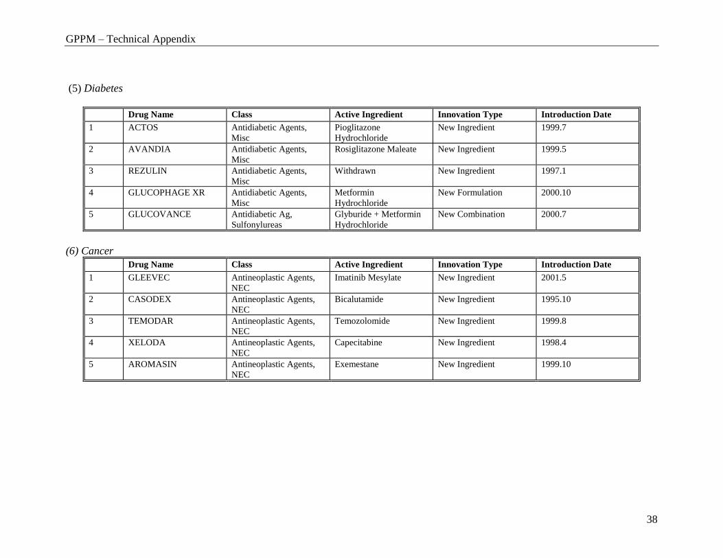
(5) Diabetes


1 ACTOS Antidiabetic Agents,

Misc

Pioglitazone

Hydrochloride


2 AVANDIA Antidiabetic Agents,

Misc

Rosiglitazone Maleate New Ingredient 1999.5

3 REZULIN Antidiabetic Agents,

Misc

Withdrawn New Ingredient 1997.1

4 GLUCOPHAGE XR Antidiabetic Agents,

Misc

Metformin

Hydrochloride


5 GLUCOVANCE Antidiabetic Ag,

Sulfonylureas

Glyburide + Metformin

Hydrochloride

New Combination 2000.7

(6) Cancer


1 GLEEVEC Antineoplastic Agents,

NEC

Imatinib Mesylate New Ingredient 2001.5

2 CASODEX Antineoplastic Agents,

NEC

Bicalutamide New Ingredient 1995.10

3 TEMODAR Antineoplastic Agents,

NEC

Temozolomide New Ingredient 1999.8

4 XELODA Antineoplastic Agents,

NEC

Capecitabine New Ingredient 1998.4

5 AROMASIN Antineoplastic Agents,

NEC

Exemestane New Ingredient 1999.10


39

(7) Depression


1 LEXAPRO Psychother,

Antidepressants

Escitalopram Oxalate New Indication 2002.8

2 PAXIL CR Psychother,

Antidepressants

Paroxetine

Hydrochloride


3 CELEXA Psychother,

Antidepressants

Citalopram

Hydrovromide


4 EFFEXOR XR Psychother,

Antidepressants

Venlafaxine

Hydrochloride


5 WELLBUTRIN SR Psychother,

Antidepressants

Buproprion

Hydrochloride



40

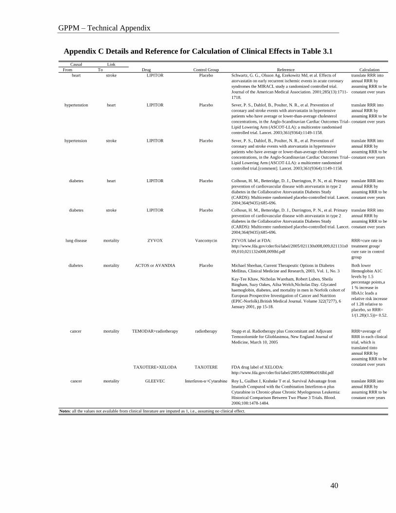
Appendix C Details and Reference for Calculation of Clinical Effects in Table 3.1

Causal Link

From To Drug Control Group Reference Calculation

heart stroke LIPITOR Placebo Schwartz, G. G., Olsson Ag, Ezekowitz Md, et al. Effects of

atorvastatin on early recurrent ischemic events in acute coronary

syndromes the MIRACL study a randomized controlled trial.

Journal of the American Medical Association. 2001;285(13):1711-

1718.

translate RRR into

annual RRR by

assuming RRR to be

conatant over years

hypertenstion heart LIPITOR Placebo Sever, P. S., Dahlof, B., Poulter, N. R., et al. Prevention of

coronary and stroke events with atorvastatin in hypertensive

patients who have average or lower-than-average cholesterol

concentrations, in the Anglo-Scandinavian Cardiac Outcomes Trial--

Lipid Lowering Arm (ASCOT-LLA): a multicentre randomised

controlled trial. Lancet. 2003;361(9364):1149-1158.

translate RRR into

annual RRR by

assuming RRR to be

conatant over years

hypertension stroke LIPITOR Placebo Sever, P. S., Dahlof, B., Poulter, N. R., et al. Prevention of

coronary and stroke events with atorvastatin in hypertensive

patients who have average or lower-than-average cholesterol

concentrations, in the Anglo-Scandinavian Cardiac Outcomes Trial--

Lipid Lowering Arm (ASCOT-LLA): a multicentre randomised

controlled trial.[comment]. Lancet. 2003;361(9364):1149-1158.

translate RRR into

annual RRR by

assuming RRR to be

conatant over years

diabetes heart LIPITOR Placebo Colhoun, H. M., Betteridge, D. J., Durrington, P. N., et al. Primary

prevention of cardiovascular disease with atorvastatin in type 2

diabetes in the Collaborative Atorvastatin Diabetes Study

(CARDS): Multicentre randomised placebo-controlled trial. Lancet.

2004;364(9435):685-696.

translate RRR into

annual RRR by

assuming RRR to be

conatant over years

diabetes stroke LIPITOR Placebo Colhoun, H. M., Betteridge, D. J., Durrington, P. N., et al. Primary

prevention of cardiovascular disease with atorvastatin in type 2

diabetes in the Collaborative Atorvastatin Diabetes Study

(CARDS): Multicentre randomised placebo-controlled trial. Lancet.

2004;364(9435):685-696.

translate RRR into

annual RRR by

assuming RRR to be

conatant over years

lung disease mortality ZYVOX Vancomycin ZYVOX label at FDA:

http://www.fda.gov/cder/foi/label/2005/021130s008,009,021131s0

09,010,021132s008,009lbl.pdf

RRR=cure rate in

treatment group/

cure rate in control

group

diabetes mortality ACTOS or AVANDIA Placebo Michael Sheehan, Current Therapeutic Options in Diabetes

Mellitus, Clinical Medicine and Research, 2003, Vol. 1, No. 3

KayTee Khaw, Nicholas Wareham, Robert Luben, Sheila

Bingham, Suzy Oakes, Ailsa Welch,Nicholas Day. Glycated

haemoglobin, diabetes, and mortality in men in Norfolk cohort of

European Prospective Investigation of Cancer and Nutrition

(EPICNorfolk).British Medical Journal. Volume 322(7277), 6

January 2001, pp 15-18.

cancer mortality TEMODAR+radiotherapy radiotherapy Stupp et al. Radiotherapy plus Concomitant and Adjuvant

Temozolomide for Glioblastmoa, New England Journal of

Medicine, March 10, 2005

TAXOTERE+XELODA TAXOTERE FDA drug label of XELODA:

http://www.fda.gov/cder/foi/label/2005/020896s016lbl.pdf

cancer mortality GLEEVEC Interferon-α+Cytarabine Roy L, Guilhot J, Krahnke T et al. Survival Advantage from

Imatinib Compared with the Combination Interferon-α plus

Cytarabine in Chronic-phase Chronic Myelogenous Leukemia:

Historical Comparison Between Two Phase 3 Trials. Blood.

2006;108:1478-1484.

translate RRR into

annual RRR by

assuming RRR to be

conatant over years

Both lower

Hemoglobin A1C

levels by 1.5

percentage points,a

1 % increase in

HbA1c leads a

relative risk increase

of 1.28 relative to

placebo, so RRR=

1/(1.28)(1.5))= 0.52.

RRR=average of

RRR in each clinical

trial, which is

translated tinto

annual RRR by

assuming RRR to be

conatant over years

Notes: all the values not available from clinical literature are imputed as 1, i.e., assuming no clinical effect.

Documents

Global Pharmaceutical Policy Model (GPPM) Technical …healthpolicy.usc.edu/documents/GPPM Technical Appendix...is applied to the change in market size between 2014 and 2015 to estimate