Global robust stabilization of cascaded polynomial systems

Systems & Control Letters 47 (2002) 445–453www.elsevier.com/locate/sysconle

Global robust stabilization of cascaded polynomial systemsZhiyong Chen, Jie Huang∗

Department of Automation and Computer-Aided Engineering, The Chinese University of Hong Kong,Shatin, NT, Hong Kong, China

Received 18 January 2002; received in revised form 26 June 2002; accepted 5 August 2002

Abstract

Global robust stabilization of nonlinear cascaded systems is a challenging problem when the zero-dynamics is notexponentially stable. Recently, some recursive procedure has been developed for handling this problem utilizing the smallgain theorem. However, the success of the procedure depends on the satisfaction of some conditions which arise at eachstep of the recursion. In this paper, we will show that, for the important class of cascaded polynomial systems, thesolvability conditions can be made satis4ed by appropriately implementing the recursive procedure. This result leads toan explicit construction of the control law.c© 2002 Elsevier Science B.V. All rights reserved.

Keywords: Global stabilization; Robust stabilization; Nonlinear control; Nonlinear systems; Polynomial systems

1. Introduction and preliminaries

We consider the class of cascaded nonlinear systems described as follows:

z =f(z; x1; �);

x1 =f1(z; x1; �) + g1(z; x1; �)x2;

...

xr =fr(z; x1; : : : ; xr ; �) + gr(z; x1; : : : ; xr ; �)u; (1.1)

where z ∈Rm; xi ∈R; i = 1; : : : ; r; u∈R, and �∈P ⊂ Rp is a vector of unknown parameters with P aprescribed compact set containing the origin of Rp. Also, the functions f;fi; gi; i = 1; : : : ; r, are suAcientlysmooth satisfying f(0; 0; �) = 0; fi(0; : : : ; 0; �) = 0; i= 1; : : : ; r, for all �∈P. It is assumed that (1.1) satis4esthe following two hypotheses:

H1: For each �, the subsystem z = f(z; x1; �) is input-to-state stable (ISS) with z as state and x1 as input,and, in particular, a class K∞ function �(·), locally Lipschitz at the origin, and independent of �, is known

∗ Corresponding author. Tel.: +85226098473; fax: +85226036002.E-mail addresses: [email protected] (Z. Chen), [email protected] (J. Huang).

0167-6911/02/$ - see front matter c© 2002 Elsevier Science B.V. All rights reserved.PII: S0167 -6911(02)00233 -5

mailto:[email protected]

mailto:[email protected]

446 Z. Chen, J. Huang / Systems & Control Letters 47 (2002) 445–453

such that the response z(·) to any bounded x1(·) satis4es

‖z(t)‖6max{�(‖z(0)‖; t); �(‖x1(·)‖∞)}; t¿ 0 (1.2)

for some class KL function �(·; ·).

H2: For i = 1; : : : ; r, there exist real numbers bi ¿ 0 such that gi(z; x1; : : : ; xi; �)¿ bi for all z; x1; : : : ; xi andall �∈P.

Remark 1.1. A nonlinear small gain theorem was given in [7,6] for a class of nonlinear systems that include(1.1) as a special case. Based on the small gain theorem, the state feedback global robust stabilization problemfor this class of systems was further investigated by means of a recursive procedure in [5–7]. At each stepof the recursion, the procedure will lead to a subsystem of the following form:

z = ’(z; x; �);

x = �(z; x; �) + (z; x; �)u (1.3)

in which (z; x)∈Rm×R; ’(0; 0; �)=0; �(0; 0; �)=0 for �∈P ⊂ Rp. The success of this procedure dependson whether or not, at each step, this subsystem satis4es four conditions described in [5, Lemma 11.4.1]. Forconvenience, let us rephrase Lemma 11.4.1 of [5] as follows:

Lemma 1.2. Consider system (1.3). Suppose the following:(i) for each �, the subsystem z = ’(z; x; �) is ISS with z as state and x as input, and, in particular, a

class K∞ function �(·), independent of �, is known such that the response z(·) to any bounded x(·) satis4es

‖z(t)‖6max{�(‖z(0)‖; t); �(‖x(·)‖∞)}; t¿ 0

for some class KL function �(·; ·);(ii) there exists a number b0 ¿ 0 such that (z; x; �)¿ b0 for all (z; x)∈Rm × R and all �∈P;(iii) for all (z; x)∈Rm × R and all �∈P,

max{|�(z; x; �)|; |x| | (z; x; �)|2}6max{�0(|x|); �1(‖z‖)};where �0(·) and �1(·) are locally Lipschitzian classK functions, and (iv) the function �1(�(·)) is locallyLipschitz at the origin.

Then, there exists a smooth function �(x), with �(0) = 0, such that, under the control law

u= �(x) + v (1.4)

the closed-loop system (1.3) and (1.4), viewed as a system with input v and state (z; x), is ISS and, inparticular, a class K∞ function �(·), independent of �, is known such that the response Z(·)= col(z(·); x(·))to any bounded v(·) satis4es

‖Z(t)‖6max{�(‖Z(0)‖; t); �(‖v(·)‖∞)}; t¿ 0


Remark 1.3. Among the four conditions, the 4rst one can be made satis4ed, under assumption H1, by appro-priate design of the control law of the form (1.4), and the second one is always satis4ed under assumptionH2. But neither the procedure itself nor assumptions H1 and H2 can guarantee the satisfaction of conditions(iii) and (iv). This is because at each step, the speci4ed functions ’, and � depend not only on the functionsf;fi; gi of the original system but also on the function � designed at previous steps.

In this paper, we will focus our attention on an important class of systems of the form (1.1) with additionalassumption that the function f is polynomial in (z; x1) and the functions fi and gi; i=1; : : : ; r, are polynomial

Z. Chen, J. Huang / Systems & Control Letters 47 (2002) 445–453 447

in (z; x1; : : : ; xi) with all coeAcients depending on �. Such systems will be called polynomial systems in thesequel. We will show, within the existing framework, that for polynomial systems of the form (1.1), underassumptions H1 and H2, conditions (iii) and (iv) of Lemma 1.2 can be made satis4ed by appropriatelydesigning the control law. Moreover, if we further assume that the class K∞ function �(·) in assumption H1is in polynomial form, then, at each step of recursion, the function �(x) in (1.4) also takes a polynomialform, and can be constructed explicitly. As a result, the global robust stabilization can always be solved bya constructive approach.The signi4cance of our result is almost self-evident since the polynomial systems are fundamental nonlinear

systems, and are frequently encountered in practice. We also note that our result is also interesting for robustnonlinear output regulation problem since so far this problem can be solved basically for polynomial nonlinearsystems [1–4].

2. Basic results

In this section, we will establish some preliminary results that will lay down the foundation of our approachto be introduced in Section 3.

Lemma 2.1. For any function f(z; x; �) with (z; x)∈Rm×R, which is polynomial in (z; x), with the coe8cientsdepending on � and satis4es f(0; 0; �) = 0 for any �∈P, there exist class K polynomial functions (thuslocally Lipschitz at the origin) �0(·) and �1(·) such that

|f(z; x; �)|6max{�0(|x|); �1(‖z‖)}: (2.1)

Proof. Assume z = col(z1; : : : ; zm). Because f(z; x; �) is polynomial in z and x, there exists a positive integerk such that f(z; x; �) can be written in the following form:

f(z; x; �) =k∑

i=1

∑ni;1+···+ni;m+ni;x=i

�(ni; 1 ;:::;ni; m;ni; x)(�)zni; 11 · · · zni;mm xni; x ;

where �(·)(�) may depend on �. Since �∈P with P a compact set, there exist nonnegative integers �(·) suchthat

|�(ni; 1 ;:::;ni; m;ni; x)(�)|6 �(ni; 1 ;:::;ni; mni; x):

Therefore,

|f(z; x; �)|6k∑

i=1


�(ni; 1 ;:::;ni; m;ni; x)|z1|ni; 1 · · · |zm|ni;m |x|ni; x

6k∑

i=1


�(ni; 1 ;:::;ni; m;ni; x)‖z‖(ni; 1+···+ni;m)|x|ni; x :

Now let �0(s) = �1(s) =∑k

i=1 L�isi, where

L�i =∑

ni;1+···+ni;m+ni;x=i

�(ni; 1 ;:::;ni; m;ni; x):


Then

�0(|x|) =k∑

i=1

L�i|x|i =k∑

i=1

∑

ni;1+···+ni;m+ni;x=i

�(ni; 1 ;:::;ni; m;ni; x)

|x|i

=k∑

i=1


�(ni; 1 ;:::;ni; m;ni; x)|x|(ni; 1+···+ni;m)|x|ni; x

¿ |f(z; x; �)|; when |x|¿ ‖z‖:Similarly, we have |f(z; x; �)|6 �1(‖z‖) when |x|6 ‖z‖.

Lemma 2.2. Consider system (1.3) with �(z; x; �) and (z; x; �) polynomials in z and x. Suppose the follow-ing:(i′) For each �, the subsystem z = ’(z; x; �) in (1.3) is ISS with z as state and x as input, and, in

particular, a class K∞ function �(·), locally Lipschitz at the origin, and independent of �, is known suchthat the response z(·) to any bounded x(·) satis4es

‖z(t)‖6max{�(‖z(0)‖; t); �(‖x(·)‖∞)}; t¿ 0

for some class KL function �(·; ·).(ii′) Same as condition (ii) of Lemma 1.2.Then, there exists a su8ciently smooth function �(x), with �(0) = 0, such that, under the control law

u= �(x) + v; (2.2)

the closed-loop system (1.3) and (2.2), viewed as a system with input v and state (z; x), is ISS and, inparticular, a class K∞ function �(·), which is locally Lipschitz at the origin, and independent of �, is knownsuch that the response Z(·) = col (z(·); x(·)) to any bounded v(·) satis4es

‖Z(t)‖6max{�(‖Z(0)‖; t); �(‖v(·)‖∞)}; t¿ 0 (2.3)


Proof. By Lemma 2.1, there are class K polynomial functions �10(·); �1

1(·); �20(·), and �2

1(·) such that

|�(z; x; �)|6max{�10(|x|); �1

1(‖z‖)};

|x 2(z; x; �)|6max{�20(|x|); �2

1(‖z‖)}:Let �0(·) = �1

0(·) + �20(·), and �1(·) = �1

1(·) + �21(·). Then clearly, system (1.3) satis4es conditions (iii) and

(iv) of Lemma 1.2. As a result, system (1.3) satis4es all conditions of Lemma 1.2. Therefore, there existsa suAciently smooth function �(x) with �(0) = 0 such that, under the control law of the form (2.2), theclosed-loop system (1.3) and (2.2), viewed as a system with input v and state (z; x), is ISS and, in particular,a class K∞ function �(·), independent of �, is known such that the response Z(·) = col(z(·); x(·)) to anybounded v(·) satis4es (2.3) for some class KL function �(·; ·).It remains to show �(·) is locally Lipschitz at the origin. To this end, recall from the proof of Lemma

11.4.1 [5] that

�(r) = max{2� ◦ �v(r); �v(r)}; (2.4)

where �v(r) = dr for some positive integer d= 1=(2b0 − !) where 0¡!¡ 2b0. Next using the fact that, forany nonnegative integers, a; b; c; d,

|max(a; b)−max(c; d)|6 |a− c|+ |b− d|


yields that, for any x; y∈ [0; &], where &∈R is suAciently small,

|�(x)− �(y)|6 |2� ◦ �v(x)− 2� ◦ �v(y)|+ |2�v(x)− 2�v(y)|6 2L|�v(x)− �v(y)|+ 2|�v(x)− �v(y)|6 (2L+ 2)d|x − y|;

where L is the Lipschitz constant of function �(·) in [0; &]. So �(·) is locally Lipschitz at the origin.

Remark 2.3. In Lemma 2.2, if the class K∞ function �(·) is assumed to be polynomial function, then thefunctions �(·) in (2.2) and �(·) in (2.3) can also be polynomial. Moreover, from the proof of Lemma 11.4.1of [5], the function �(x) takes the form �(x) = −x − �(x) where �(x) is a smooth strictly increasing oddfunction satisfying

�(|x|)¿ 32b0

max{�0(|x|); �1(�(|2x|))};

where �0(·), and �1(·) are those given in the proof of Lemma 2.2. Since �0(·), and �1(·) are polynomialfunctions, it is always possible to choose �, hence �, to be a polynomial function provided the function �(·) isalso in polynomial form. In fact, it suAces to let �(x)=ax+bxp with a and b suAciently large real numbers,and p suAciently large integer. Furthermore, it suAces to choose

�(r) = 2� ◦ �v(r) + 2�v(r)

to satisfy (2.4), and, clearly, �(r) is polynomial.

3. Algorithm

Lemma 2.2 together with Remark 2.3 shows that it is always possible to give an explicit expression forcontroller (2.2). These three numbers a; b and p may depend on the size of the compact set P. We nowproceed to further construct an explicit controller to solve the problem based on the recursive algorithmsuggested in [5–7].

Theorem 3.1. Consider system (1.1), under assumptions H1 and H2, and further assume that the class K∞function �(·) in assumption H1 is in polynomial form, then the global robust stabilization problem of (1.1)is solvable.

Proof. A constructive proof will be given. Throughout this proof, denote xr+1 := u.Step 1: De4ne a subsystem of (1.1) as follows:

z = f(z; x1; �);

x1 = f1(z; x1; �) + g1(z; x1; �)x2: (3.1)

Under H1 and H2, by Lemma 2.2 and Remark 2.3 there exists a polynomial function �1(x1) such that thecoordinate transformation x1 = x1, and x2 = x2 − �1(x1) converts system (1.1) into the following:

Z1 = F1(Z1; x2; �);

˙x2 = f 2(Z1; x2; �) + g2(Z1; x2; �)x3;

xi = f1i (Z1; x2; x3; : : : ; xi; �) + g1i (Z1; x2; x3; : : : ; xi; �)xi+1; i = 3; : : : ; r; (3.2)


where Z1 = col(z; x1) and

F1(Z1; x2; �) =

[f(z; x1; �)

f1(z; x1; �) + g1(z; x1; �)(�1(x1) + x2)

];

f 2(Z1; x2; �) = f2(z; x1; x2; �)− d�(x1)dx1

(f1(z; x1; �) + g1(z; x1; �)(�1(x1) + x2));

g2(Z1; x2; �) = g2(z; x1; x2; �);

f1i (Z1; x2; x3; : : : ; xi; �) = fi(z; x1; : : : ; xi; �);

g1i (Z1; x2; x3; : : : ; xi; �) = gi(z; x1; : : : ; xi; �):

Moreover, the subsystem governing Z1 is ISS with state Z1 and input x2, and, in particular, a class K∞function �1(·), in polynomial, thus locally Lipschitz at the origin and independent of �, is known such thatthe response Z1(·) to any bounded x2(·) satis4es

‖Z1(t)‖6max{�1(‖Z1(0)‖; t); �1(‖x2(·)‖∞)}; t¿ 0

for some class KL function �1(·; ·). That is, the subsystem Z1 = F1(Z1; Lx2; �) satis4es hypothesis H1 withZ1 = z; Lx2 = x1 and F1 = f. Also, the functions f 2; g2 and f1

i ; g1i for i = 3; : : : ; r, are all polynomials.

Step j; j = 2; : : : ; r: Assume at the end of (j − 1)th step, we obtain a system of the form

Z j−1 = Fj−1(Zj−1; xj ; �);

˙xj = f j(Zj−1; xj ; �) + gj(Zj−1; xj ; �)xj+1;

xi = fj−1i (Zj−1; xj ; xj+1; : : : ; xi; �) + gj−1

i (Zj−1; xj ; xj+1; : : : ; xi; �)xi+1; i = j + 1; : : : ; r; (3.3)

where Zj−1=col(z; x1; : : : ; xj−1) and the functions f j; gj and fj−1i ; gj−1

i for i=j+1; : : : ; r, are all polynomials.Furthermore, the subsystem Z j−1=Fj−1(Zj−1; Lxj; �) satis4es hypothesis H1 with Zj−1=z; Lxj=x1 and Fj−1=fholds for a known class K∞ function �j−1(·), which is polynomial, thus locally Lipschitz at the origin, andindependent of �, for some class KL function �j−1(·; ·).

Comparing system (3.3) and (1.1) shows that these two systems have same structure satisfying the sameassumptions. So use the same analysis as that in step 1 on system (3.3), it is easy to obtain that there exists asuAciently smooth function �j(xj) such that the coordinate transformation xj+1=xj+1−�j(xj) converts system(3.3) into the following:

Z j = Fj(Zj; xj+1; �);

˙xj+1 = f j+1(Zj; xj+1; �) + gj+1(Zj; xj+1; �)xj+2;

xi = fji (Zj; xj+1; xj+2; : : : ; xi; �) + gj

i (Zj; xj+1; xj+2; : : : ; xi; �)xi+1; i = j + 2; : : : ; r; (3.4)

where Zj = col(z; x1; : : : ; xj) and the functions f j+1; gj+1 and fji ; g

ji for i = j + 2; : : : ; r are all polynomials.

Furthermore, the subsystem Z j = Fj(Zj; Lxj+1; �) satis4es hypothesis H1 with Zj = z; Lxj+1 = x1 and Fj =f fora known class K∞ function �j(·), which is polynomial, thus locally Lipschitz at the origin, and independentof �, for some class KL function �j(·; ·).

Step r + 1: At the end of step r, one has obtained a system

Z r = Fr(Zr; xr+1; �) (3.5)


with Zr = col(z; x1; : : : ; xr), and (3.5) is ISS with state Zr and input xr+1. Thus letting xr+1 = 0 shows thatthe origin of system Z r = Fr(Zr; 0; �) is globally asymptotically stable for all �∈P: Or what is the same, theoriginal system (1.1) is globally asymptotically stable under control u= �r(xr) since xr+1 = xr+1− �r(xr). Theoverall controller expressed in the original coordinate is given by

u= �r(xr);

xi = xi − �i−1(xi−1); i = r; : : : ; 2;

x1 = x1: (3.6)

Remark 3.2. If, for some i∈{1; : : : ; r}, there exists real number bi ¡ 0 such that gi(z; x1; : : : ; xi; �)6 bi for allx1; : : : ; xi; z and all �∈P, Theorem 3.1 still holds. And, if the upper subsystem of (1.1) is not in polynomialform, that is, the function f is not polynomial, Theorem 3.1 still holds.

Remark 3.3. It should be noted that the global stabilization problem for the lower triangular system of theform (1.1) has also been studied under some other assumptions [8,9]. In particular, in [8], under the assumptionthat the zero dynamics of system (1.1) is globally asymptotically stable (GAS) and locally exponentially stable(LES), a full state feedback control law can be constructed by a backstepping procedure. Nevertheless, ourresult here can handle some cases that do not satisfy the LES assumption as will be seen from the examplein the next section.

Remark 3.4. It can be veri4ed that it suAces to assume hypotheses H1 and H2 in order to guarantee thesolvability of the global robust stabilization for the polynomial systems of the form (1.1). The additionalassumption that the class K∞ function �(·) in hypothesis H1 is a polynomial further leads to the explicitconstruction of a family of control laws in polynomial form.

Remark 3.5. Note that, even for polynomial systems with ISS property, the class K∞ function �(·) mentionedin H1 may not be polynomial, and may not even be Locally Lipschitzian. For example, consider the system

x1 =−x31 + x1x2

which is ISS with state x1 and input x2. An estimate of the form (1.2) holds with �(r) =√r=(

√1− !) for

any 0¡!¡ 1. But �(·) is neither polynomial nor Locally Lipschitzian.

4. Example

Consider the following lower-triangular system:

z =−z3 + �1z2x1;

x1 = 14x

21 +

16x1z + �1z + 2x2;

x2 = x21z + 2x1z2 − �2x2 + 5(�23 + 1)u: (4.1)

We will design a state-feedback controller to globally stabilize this system in the presence of three uncertainparameters �1; �2; �3.For this purpose, we need to check whether or not the subsystem z=−z3+�1z2x1 of (4.1) satis4es H1. This

is indeed the case with the function �(|x1|) = |x1|, though the system with x1 = 0 is not locally exponentiallystable. Thus by Theorem 3.1, system (4.1) is globally stabilizable with a control law in polynomial form. Toexplicitly derive our control law, we assume �1; �2; �3 ∈ [− 1; 1].


At the 4rst step, consider the subsystem out of (4.1) as follows:

z =−z3 + �1z2x1;

x1 = 14x

21 +

16x1z + �1z + 2x2: (4.2)

with x2 as the input and (z; x1) as the state. Let

�0(|x1|) = 13 |x1|2 + 4|x1|; �1(|z|) = 1

3 |z|2 + |z|:Then

max{| 14x21 + 16x1z + �1z|; 4|x1|}6max{�0(|x1|); �1(|z|)}:

It is easy to verify that �1(x1) = x31 + 4x1 satis4es:

�1(|x1|)¿ |x1|2 + 3|x1|¿ 32× 2

max{�0(|x1|); �1(�(|2x1|))}:

So under controller x2 = �1(x1) + x2 with �1(x1) =−x1 − �1(x1) =−x31 − 5x1 system (4.2) is ISS with (z; x1)as state and x2 as input, and, in particular the estimate �1 can be calculated as �1(r) = r.This controller de4nes a coordinate transformation x1 =x1 and x2 =x2 +x31 +5x1 which converts the original

system (4.1) into the following:

z =−z3 + �1z2x1;

˙x1 = 14 x21 +

16 x1z + �1z − 2x31 − 10x1 + 2x2;

˙x2 = x21z + 2x1z2 − �2(x2 − x31 − 5x1) + (3x21 + 5) ˙x1 + 5(�23 + 1)u: (4.3)

To proceed to the second (hence the last) step, denote Z1 = col(z; x1). Then it can be veri4ed that

|x21z + 2x1z2 − �2(x2 − x31 − 5x1) + (3x21 + 5) ˙x1|6 6‖Z1‖5 + 5

4‖Z1‖4 + 47‖Z1‖3 + 2512‖Z1‖2 + 60‖Z1‖+ 6‖Z1‖2|x2|+ 11|x2|:

Let

�0(|x2|) = 6|x2|5 + 54 |x2|4 + 53|x2|3 + 25

12 |x2|2 + 100|x2|;

�1(‖Z1‖) = 6‖Z1‖5 + 54‖Z1‖4 + 53‖Z1‖3 + 25

12‖Z1‖2 + 100‖Z1‖:Then

max{|x21z + 2x1z2 − �2(x2 − x31 − 5x1) + (3x21 + 5) ˙x1|; 25|x2|(�23 + 1)2}6max{�0(|x2|); �1(‖Z1‖)}:

It is easy to verify that �2(x2) = 32 (2x2)

5 + 9(2x2)3 + 25(2x2)− x2 satis4es

�1(|x2|)¿ 32× 10

max{�0(|x2|); �1(�1(|2x2|))}:

So under controller u= �2(x2) with �2(x2) =−x2 − �2(x2) =− 32 (2x2)

5 − 9(2x2)3 − 25(2x2) system (4.1) canbe globally stabilized.The overall controller for solving the global robust stabilization problem for system (4.1) is thus given by

u=− 32 (2x2)

5 − 9(2x2)3 − 25(2x2);

x2 = x2 + x31 + 5x1:

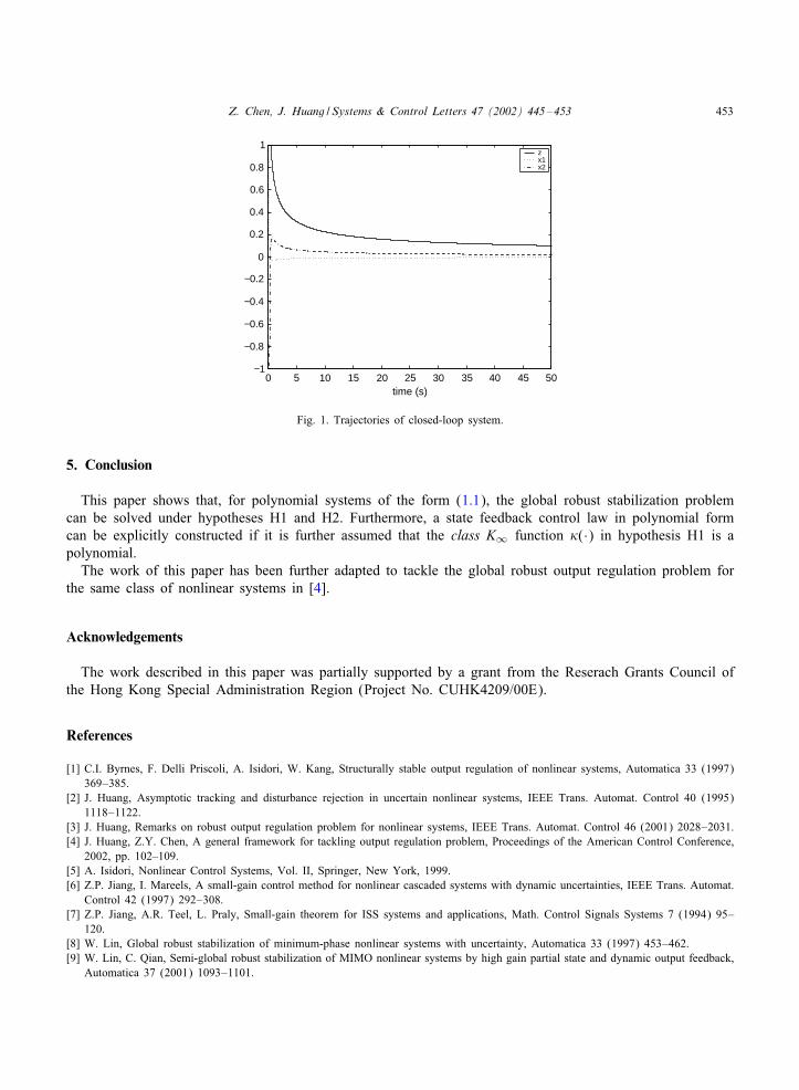
Fig. 1 shows the trajectories of the states for the case where

z(0) = x1(0) = x2(0) = 100; �1 =−0:4; �2 = 0:8; �3 = 0:3:


0 5 10 15 20 25 30 35 40 45 50−1

−0.8

−0.6

−0.4

−0.2

0

0.2

0.4

0.6

0.8

1zx1x2

time (s)

Fig. 1. Trajectories of closed-loop system.

5. Conclusion

This paper shows that, for polynomial systems of the form (1.1), the global robust stabilization problemcan be solved under hypotheses H1 and H2. Furthermore, a state feedback control law in polynomial formcan be explicitly constructed if it is further assumed that the class K∞ function �(·) in hypothesis H1 is apolynomial.The work of this paper has been further adapted to tackle the global robust output regulation problem for

the same class of nonlinear systems in [4].

Acknowledgements

The work described in this paper was partially supported by a grant from the Reserach Grants Council ofthe Hong Kong Special Administration Region (Project No. CUHK4209/00E).

References

[1] C.I. Byrnes, F. Delli Priscoli, A. Isidori, W. Kang, Structurally stable output regulation of nonlinear systems, Automatica 33 (1997)369–385.

[2] J. Huang, Asymptotic tracking and disturbance rejection in uncertain nonlinear systems, IEEE Trans. Automat. Control 40 (1995)1118–1122.

[3] J. Huang, Remarks on robust output regulation problem for nonlinear systems, IEEE Trans. Automat. Control 46 (2001) 2028–2031.[4] J. Huang, Z.Y. Chen, A general framework for tackling output regulation problem, Proceedings of the American Control Conference,

2002, pp. 102–109.[5] A. Isidori, Nonlinear Control Systems, Vol. II, Springer, New York, 1999.[6] Z.P. Jiang, I. Mareels, A small-gain control method for nonlinear cascaded systems with dynamic uncertainties, IEEE Trans. Automat.

Control 42 (1997) 292–308.[7] Z.P. Jiang, A.R. Teel, L. Praly, Small-gain theorem for ISS systems and applications, Math. Control Signals Systems 7 (1994) 95–

120.[8] W. Lin, Global robust stabilization of minimum-phase nonlinear systems with uncertainty, Automatica 33 (1997) 453–462.[9] W. Lin, C. Qian, Semi-global robust stabilization of MIMO nonlinear systems by high gain partial state and dynamic output feedback,

Automatica 37 (2001) 1093–1101.

Documents

Global robust stabilization of cascaded polynomial systems