Embed Size (px)
Citation preview
Global Search Regression (GSREG): A new
automatic model selection technique for cross-
section, time series and panel data regressions1
Pablo Gluzmann DemianPanigo
CONICET-CEDLAS, UNLP CEIL-CONICET, UNM, UNLP
La Plata, Argentina La Plata, Argentina
[email protected] [email protected]
Abstract. This paper presents the main features of Global
Search Regression (GSREG), a new automatic model
selection technique (AMST) for time series, cross-section and
panel data regressions. As other exhaustive search
algorithms (e.g. VSELECT) GSREG avoids characteristic
path-dependence traps of standard backward and forward
looking approaches (like PCGETS or RETINA). However,
GSREG is the first STATA® code that: 1) guarantees
optimality with out-of-sample selection criteria; 2) allows
residual testing for each alternative; 3) retains VSELECT
leaps-and-bound “shortcuts” for in-sample selection criteria;
and 4) provides (depending on user specifications) a full-
information dataset with outcome statistics for every
alternative model.
Keywords: GSREG, automatic model selection, VSELECT,
PC-GETS, RETINA.
JEL Codes: C10, C52, C87.
1GSREG was based on FUERZA_BRUTA, a former Stata .do file originally developed
by Demian Panigo and subsequently enhanced by Diego Herrero (UBA, Argentina) and
Pablo Gluzmann. Usual disclaimer applies.
2
1 Introduction.
Econometric practitioners are commonly faced with global
optimization issues. Identifying the real data generating process (DGP)
from a myriad of alternative econometric models is analogous to looking
for a global minimum in a highly non-linear optimization problem. In
both cases, some broadly accepted procedures lead to wrong or
improvable results.2
While global optimization methods in mathematics evolved, for
example, from Rawson-Newton to genetic algorithms (and related
search strategies), econometric model selection techniques have been
changing from rudimentary (backward and/or forward STEPWISE)
sequential regressions to more sophisticated approaches (PC-GETS,
RETINA, LARS, LASSO; see Castle, 2006)
Even though, sub-optimal path-dependent results still (and
frequently) emerge. Like genetic algorithms in global optimization
problems, most AMSTs cannot guarantee a “global optimum” (the best
DGP from available alternatives) in model selection. Different final
outcomes can be obtained depending on both search parameters
(crucially test parameters) and search starting points (see Derksen and
Keselman, 1992).
Newer AMSTs like PC-GETS or RETINA intended to avoid this
problem by means of alternative multi path – multi sample backward
and forward looking approaches, respectively. While these strategies
have significantly improve AMSTs outcomes (Marinucci, 2008), they still
fail to guarantee “global optima” because of unexplored reduction paths,
the size-power trade-off and cumulative type-I errors of sequential
testing, especially in small sample problems.
The combination of non-exhaustive search (like single or multiple
path search strategies) and sequential testing (either forward or
backward looking) will frequently afford some cost in term of statistical
inference (depending of test size and selected paths, it will take the form
of model under or overfitting) and just by chance the “terminal model”
will coincide with the best DGP.
These weaknesses, altogether with increasing computational
capabilities explain the widening use of alternative exhaustive search
methods. Unlike global optimum search in mathematics3, a model 2 In econometrics, Leamer (1978) and Lovell (1983) documented the low success rates
of many widely used model selection techniques, while, Forrest and Mitchell (1993)
stress the limitations of new “standards” (e.g. genetic algorithms) in the numerical
optimization. 3 The meaning of exhaustive search in mathematics (e.g. in non-linear optimization
problems) is not completely satisfactory. Algorithms like PATTERN SEARCH in
Matlab© provide a useful example to understand what exhaustive search actually
3
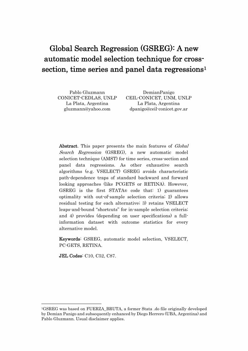
selection problem in econometrics is always self-constrained. The
number of point (models) to be evaluated will never be infinite but a
certain integer defined by 2n, where n is the number of initially
admissible covariates. This quantity, while exponentially increasing in
n, is by far much more manageable than any unconstrained non-linear
global optimization problem.
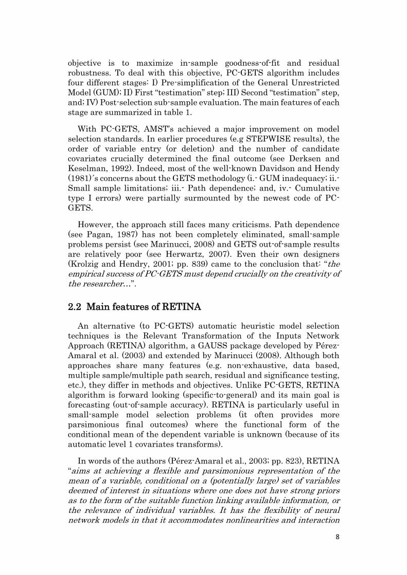
Figure 1.- Exhaustive search: Alternative models to be evaluated at
different number of initially admissible covariates
All in all, the choice between exhaustive and non-exhaustive search
is determined by the trade-off between time and accuracy. Last
generation AMSTs try to take into account both dimensions, standing
somewhere between pure time saving techniques (e.g. first generation
AMSTs like STEPWISE regressions) and pure accuracy improving
methods (exhaustive search). This shows that AMST evolution goes from
speed to goodness-of-fit, as long as processing power innovation
increases computational capabilities.
In a recent post (http://www.stata.com/why-use-stata/fast), Stata
Corporation states that on a Intel® 2.4 GHz Core 2 Quad with Stata/SE
for Windows 7, running a linear regression on 10 covariates and 10,000
observations takes 0.034 seconds. Exhaustive search of the best DGP in
means in a global optimization context. Indeed, the PATTERN SEARCH algorithm
iterative looks for a global minimum in variable-size mesh until a threshold level is
attained. However, without constraints the problem had to be evaluated at an infinite
number of points. Using polling method options, the PATTERN SEARCH algorithm
reduces the number of iterations to a convenient dimension. Nevertheless, the stronger
the constraint, the higher the loss of the global minimum accuracy.
1
10
100
1,000
10,000
100,000
1,000,000
10,000,000
100,000,000
2 4 6 8 10 12 14 16 18 20 22 24
Num
ber
of m
odel
s to
be
evalu
ate
d (
logari
thm
ic s
cale
)
Number of potent ially admissible covariates
4
the same example (10,000 observation and 10 covariates) will involve
1,024 linear regressions in about 34 seconds. Moreover, using one of the
last Intel® Xeon® processors (Xeon® X5698, 2011, 4.4 GHz) the same
procedure will take just 19.3 seconds.
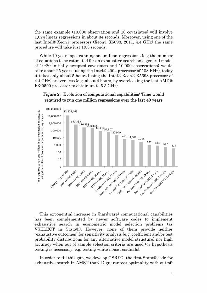
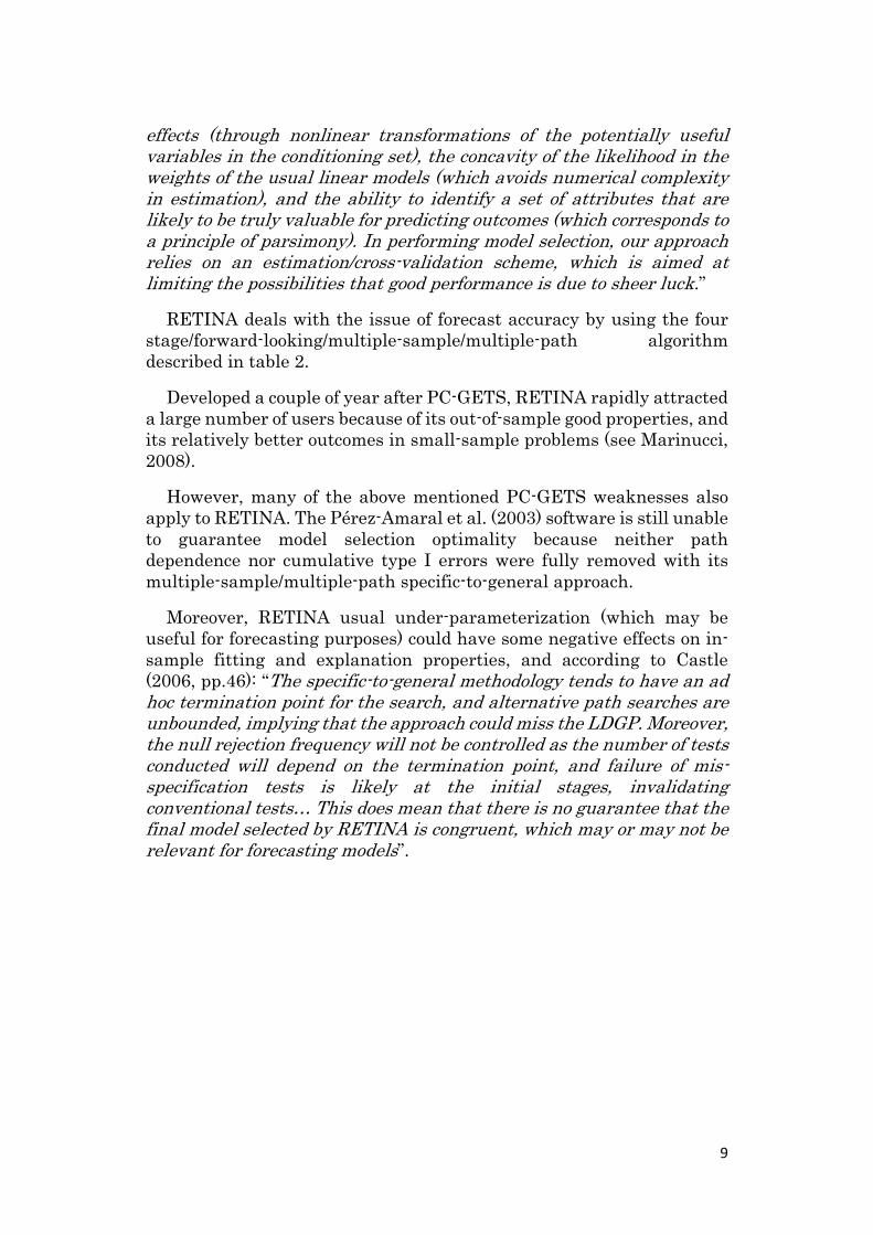
While 40 years ago, running one million regressions (e.g the number
of equations to be estimated for an exhaustive search on a general model
of 19-20 initially accepted covariates and 10,000 observations) would
take about 25 years (using the Intel® 4004 processor of 108 KHz), today
it takes only about 5 hours (using the Intel® Xeon® X5698 processor of
4.4 GHz) or even less (e.g. about 4 hours, by overclocking the last AMD®
FX-9590 processor to obtain up to 5.3 GHz).
Figure 2.- Evolution of computational capabilities: Time would
required to run one million regressions over the last 40 years
This exponential increase in (hardware) computational capabilities
has been complemented by newer software codes to implement
exhaustive search in econometric model selection problems (as
VSELECT in Stata®). However, none of them provide neither
“exhaustive outcomes” for sensitivity analysis (e.g. coefficient and/or test
probability distributions for any alternative model structure) nor high
accuracy when out-of-sample selection criteria are used (or hypothesis
testing is necessary: e.g. testing white noise residuals).
In order to fill this gap, we develop GSREG, the first Stata® code for
exhaustive search in AMST that: 1) guarantees optimality with out-of-
12,802,469
691,333276,533
230,44486,41755,307
20,9496,913 4,609
2,765922 813 567
314
1
10
100
1,000
10,000
100,000
1,000,000
10,000,000
100,000,000
Tim
e r
eq
uir
ed
to r
un
on
e m
illio
n l
ine
ar r
egr
ess
ion
in S
tata
/SE,
u
sin
g d
iffe
ren
t In
tel
Pro
cess
ors
(in
min
ute
s, l
og.
sca
le)
5
sample selection criteria; 2) allows residual behavior testing for each
alternative; 3) retains VSELECT branch-and-bound “shortcuts” for in-
sample selection criteria; and 4) provides (depending on user
specifications) a full-information dataset with outcome statistics for
every alternative model.4
In what follows, we structure the paper in 5 sections. First, we discuss
strengths and weaknesses of main automatic model selection
approaches. Next, we introduce the main characteristic GSREG
(algorithm, stages and uses). In section 4 the syntax is reproduced,
complemented with section 5 in which different options are explained.
Then, some examples are presented to facilitate user first contact with
GSREG. Section 7 is used to describe the features of saved results, while
the last two sections are devoted to acknowledgments and
bibliographical references.
2 Distinctive features of main AMSTs
By combining and extending Hendry’s (1980); Miller’s (1984);
Gatuand Kontoghiorghes’ (2006) and Duarte Silva’s (2009)
categorizations, it is possible to generate the following “conceptual tree”
of model selection techniques:
4 GSREG will initially be used for small-size problems in standard personal computers
(e.g. to find the best DGP over different combinations of 20 or less potential covariates,
which can be solved in a couple of hours). However, larger calculations will soon be
manageable, because a “parallelization revolution” is coming soon. A few years from
now, it will be unsurprising to solve a one-billion regression problem with GSREG in
two hours using GPGPU computing and CUDA/OPENCL-like reengineering to
improve GSREG parallelization capabilities (e.g. to fully exploit the PART option
potential).
6
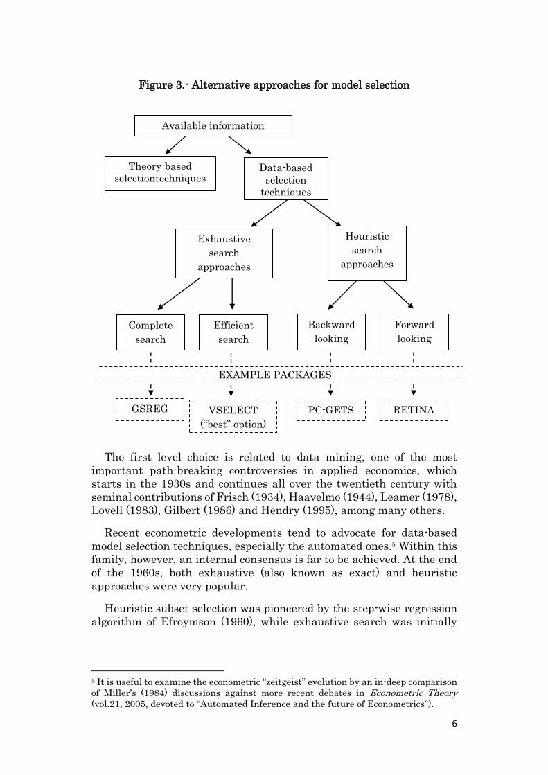
Figure 3.- Alternative approaches for model selection
The first level choice is related to data mining, one of the most
important path-breaking controversies in applied economics, which
starts in the 1930s and continues all over the twentieth century with
seminal contributions of Frisch (1934), Haavelmo (1944), Leamer (1978),
Lovell (1983), Gilbert (1986) and Hendry (1995), among many others.
Recent econometric developments tend to advocate for data-based
model selection techniques, especially the automated ones.5 Within this
family, however, an internal consensus is far to be achieved. At the end
of the 1960s, both exhaustive (also known as exact) and heuristic
approaches were very popular.
Heuristic subset selection was pioneered by the step-wise regression
algorithm of Efroymson (1960), while exhaustive search was initially
5 It is useful to examine the econometric “zeitgeist” evolution by an in-deep comparison
of Miller’s (1984) discussions against more recent debates in Econometric Theory
(vol.21, 2005, devoted to “Automated Inference and the future of Econometrics”).
Theory-based
selectiontechniques
Available information
Exhaustive
search
approaches
Data-based
selection
techniques
EXAMPLE PACKAGES
Complete
search
Efficient
search
Backward
looking
Forward
looking
GSREG VSELECT
(“best” option)
PC-GETS RETINA
Heuristic
search
approaches
7
associated with the “optimal/complete regression” strategy of Coen,
Gomme and Kendall (1969).
Box and Newbold (1971) criticisms on exhaustive search techniques
(e.g. they are unfeasible for large-size problems), and Berk (1978)
objections on stepwise algorithms (e.g. they do not guarantee optimality)
have brought a growing consensus on the need for better alternatives.
The number of newer exhaustive and heuristic model selection
techniques grew exponentially in the past forty years. Alternative
algorithms arose, such as Non-negative Garrote (Breiman, 1995),
LASSO (Tibshirani, 1996); LARS (Efron, Hastie, Johnstone and
Tibshirani, 2004); VSELECT-Leaps and Bound (Furnival and Wilson,
1974; Lindsey and Sheter, 2010); PCGETS/AUTOMETRICS (Krolzig
and Hendry, 2001, Doornik, 2008); and RETINA (Pérez-Amaral et al.,
2003).
To provide a proper context to introduce GSREG, the following sub-
section briefly discuss the main properties of most commonly used
AMSTs
2.1 Main features of PC-GETS6
Following Hoover’s (2006, pp. 76) definition, the GETS approach
“involves starting with as broad a general specification as possible and then searching over the space of possible restrictions to find the most parsimonious specification. At each step in a sequential reduction (usually along multiple paths), the statistical properties of the errors are tested, the validity of the reduction is tested statistically both against the immediate predecessor and the general specification, and encompassing is tested against all otherwise satisfactory alternative specifications.”
While some features of the GETS-LSE methodology have been used
in commercial econometric packages since the 1980s, it was not until
Krolzig and Hendry (2001) developed PC-GETS (written in OX
language) that this methodology was fully automated with a multiple-
sample/multiple-path/backward looking algorithm.
Although it is flexible enough to be applied to many other alternatives
(see Castle, 2006), PC-GETS is mainly employed in big model selection
problems (e.g. many covariates and large databases) where the main
6In spite of the fact that OxMetrics™ has recently announced the replacement of PC-
GETS by AUTOMETRICS, we discuss in this section the main features of the former
because: 1) there is much more academic research on it, allowing pros and cons
evaluation, and; 2) they share the “core algorithm” and the only difference is that
AUTOMETRICS uses a tree search method, with improvements on pre-search
simplification and on the objective function (see Doornik, 2008).
8
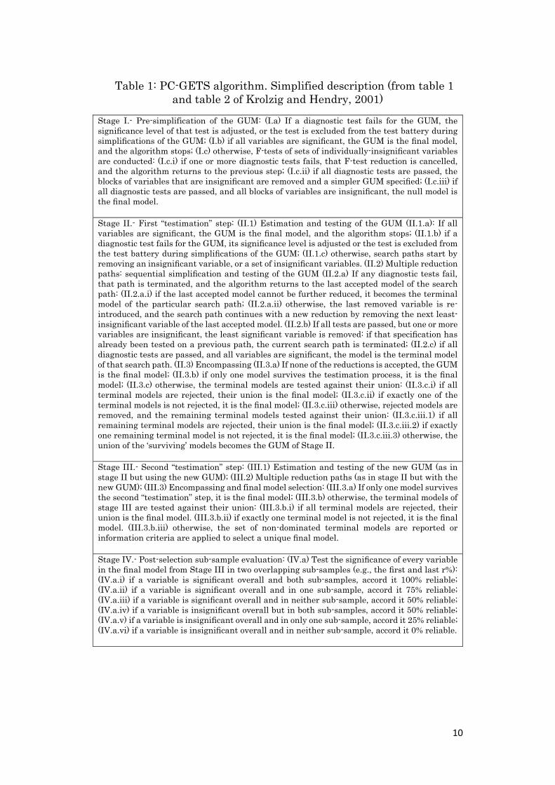
objective is to maximize in-sample goodness-of-fit and residual
robustness. To deal with this objective, PC-GETS algorithm includes
four different stages: I) Pre-simplification of the General Unrestricted
Model (GUM); II) First “testimation” step; III) Second “testimation” step,
and; IV) Post-selection sub-sample evaluation. The main features of each
stage are summarized in table 1.
With PC-GETS, AMST’s achieved a major improvement on model
selection standards. In earlier procedures (e.g STEPWISE results), the
order of variable entry (or deletion) and the number of candidate
covariates crucially determined the final outcome (see Derksen and
Keselman, 1992). Indeed, most of the well-known Davidson and Hendy
(1981)´s concerns about the GETS methodology (i.- GUM inadequacy; ii.-
Small sample limitations; iii.- Path dependence; and, iv.- Cumulative
type I errors) were partially surmounted by the newest code of PC-
GETS.
However, the approach still faces many criticisms. Path dependence
(see Pagan, 1987) has not been completely eliminated, small-sample
problems persist (see Marinucci, 2008) and GETS out-of-sample results
are relatively poor (see Herwartz, 2007). Even their own designers
(Krolzig and Hendry, 2001; pp. 839) came to the conclusion that: “the empirical success of PC-GETS must depend crucially on the creativity of the researcher…”.
2.2 Main features of RETINA
An alternative (to PC-GETS) automatic heuristic model selection
techniques is the Relevant Transformation of the Inputs Network
Approach (RETINA) algorithm, a GAUSS package developed by Pérez-
Amaral et al. (2003) and extended by Marinucci (2008). Although both
approaches share many features (e.g. non-exhaustive, data based,
multiple sample/multiple path search, residual and significance testing,
etc.), they differ in methods and objectives. Unlike PC-GETS, RETINA
algorithm is forward looking (specific-to-general) and its main goal is
forecasting (out-of-sample accuracy). RETINA is particularly useful in
small-sample model selection problems (it often provides more
parsimonious final outcomes) where the functional form of the
conditional mean of the dependent variable is unknown (because of its
automatic level 1 covariates transforms).
In words of the authors (Pérez-Amaral et al., 2003; pp. 823), RETINA
“aims at achieving a flexible and parsimonious representation of the mean of a variable, conditional on a (potentially large) set of variables deemed of interest in situations where one does not have strong priors as to the form of the suitable function linking available information, or the relevance of individual variables. It has the flexibility of neural network models in that it accommodates nonlinearities and interaction
9
effects (through nonlinear transformations of the potentially useful variables in the conditioning set), the concavity of the likelihood in the weights of the usual linear models (which avoids numerical complexity in estimation), and the ability to identify a set of attributes that are likely to be truly valuable for predicting outcomes (which corresponds to a principle of parsimony). In performing model selection, our approach relies on an estimation/cross-validation scheme, which is aimed at limiting the possibilities that good performance is due to sheer luck.”
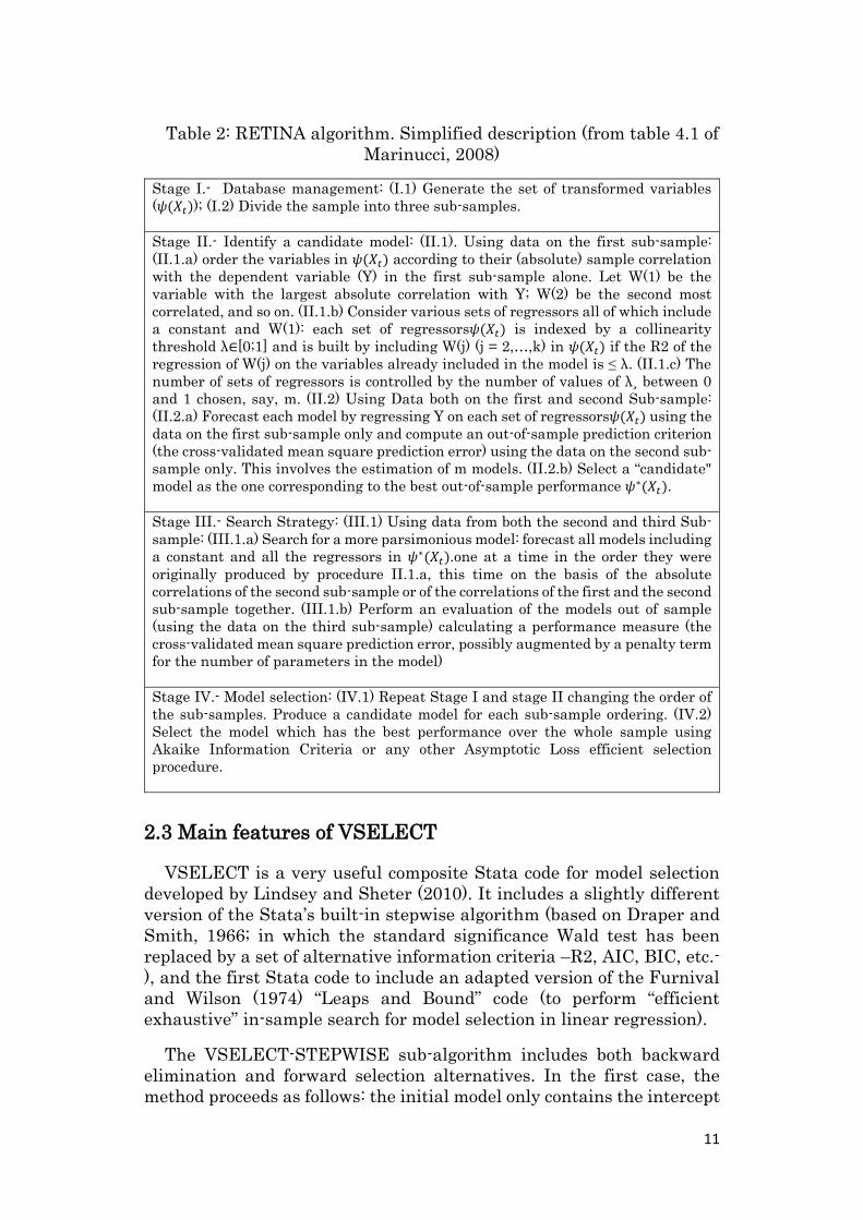
RETINA deals with the issue of forecast accuracy by using the four
stage/forward-looking/multiple-sample/multiple-path algorithm
described in table 2.
Developed a couple of year after PC-GETS, RETINA rapidly attracted
a large number of users because of its out-of-sample good properties, and
its relatively better outcomes in small-sample problems (see Marinucci,
2008).
However, many of the above mentioned PC-GETS weaknesses also
apply to RETINA. The Pérez-Amaral et al. (2003) software is still unable
to guarantee model selection optimality because neither path
dependence nor cumulative type I errors were fully removed with its
multiple-sample/multiple-path specific-to-general approach.
Moreover, RETINA usual under-parameterization (which may be
useful for forecasting purposes) could have some negative effects on in-
sample fitting and explanation properties, and according to Castle
(2006, pp.46): “The specific-to-general methodology tends to have an ad hoc termination point for the search, and alternative path searches are unbounded, implying that the approach could miss the LDGP. Moreover, the null rejection frequency will not be controlled as the number of tests conducted will depend on the termination point, and failure of mis-specification tests is likely at the initial stages, invalidating conventional tests… This does mean that there is no guarantee that the final model selected by RETINA is congruent, which may or may not be relevant for forecasting models”.
10
Table 1: PC-GETS algorithm. Simplified description (from table 1
and table 2 of Krolzig and Hendry, 2001)
Stage I.- Pre-simplification of the GUM: (I.a) If a diagnostic test fails for the GUM, the
significance level of that test is adjusted, or the test is excluded from the test battery during
simplifications of the GUM; (I.b) if all variables are significant, the GUM is the final model,
and the algorithm stops; (I.c) otherwise, F-tests of sets of individually-insignificant variables
are conducted: (I.c.i) if one or more diagnostic tests fails, that F-test reduction is cancelled,
and the algorithm returns to the previous step; (I.c.ii) if all diagnostic tests are passed, the
blocks of variables that are insignificant are removed and a simpler GUM specified; (I.c.iii) if
all diagnostic tests are passed, and all blocks of variables are insignificant, the null model is
the final model.
Stage II.- First “testimation” step: (II.1) Estimation and testing of the GUM (II.1.a): If all
variables are significant, the GUM is the final model, and the algorithm stops; (II.1.b) if a
diagnostic test fails for the GUM, its significance level is adjusted or the test is excluded from
the test battery during simplifications of the GUM; (II.1.c) otherwise, search paths start by
removing an insignificant variable, or a set of insignificant variables. (II.2) Multiple reduction
paths: sequential simplification and testing of the GUM (II.2.a) If any diagnostic tests fail,
that path is terminated, and the algorithm returns to the last accepted model of the search
path: (II.2.a.i) if the last accepted model cannot be further reduced, it becomes the terminal
model of the particular search path; (II.2.a.ii) otherwise, the last removed variable is re-
introduced, and the search path continues with a new reduction by removing the next least-
insignificant variable of the last accepted model. (II.2.b) If all tests are passed, but one or more
variables are insignificant, the least significant variable is removed: if that specification has
already been tested on a previous path, the current search path is terminated; (II.2.c) if all
diagnostic tests are passed, and all variables are significant, the model is the terminal model
of that search path. (II.3) Encompassing (II.3.a) If none of the reductions is accepted, the GUM
is the final model; (II.3.b) if only one model survives the testimation process, it is the final
model; (II.3.c) otherwise, the terminal models are tested against their union: (II.3.c.i) if all
terminal models are rejected, their union is the final model; (II.3.c.ii) if exactly one of the
terminal models is not rejected, it is the final model; (II.3.c.iii) otherwise, rejected models are
removed, and the remaining terminal models tested against their union: (II.3.c.iii.1) if all
remaining terminal models are rejected, their union is the final model; (II.3.c.iii.2) if exactly
one remaining terminal model is not rejected, it is the final model; (II.3.c.iii.3) otherwise, the
union of the ‘surviving’ models becomes the GUM of Stage II.
Stage III.- Second “testimation” step: (III.1) Estimation and testing of the new GUM (as in
stage II but using the new GUM); (III.2) Multiple reduction paths (as in stage II but with the
new GUM); (III.3) Encompassing and final model selection: (III.3.a) If only one model survives
the second “testimation” step, it is the final model; (III.3.b) otherwise, the terminal models of
stage III are tested against their union: (III.3.b.i) if all terminal models are rejected, their
union is the final model. (III.3.b.ii) if exactly one terminal model is not rejected, it is the final
model. (III.3.b.iii) otherwise, the set of non-dominated terminal models are reported or
information criteria are applied to select a unique final model.
Stage IV.- Post-selection sub-sample evaluation: (IV.a) Test the significance of every variable
in the final model from Stage III in two overlapping sub-samples (e.g., the first and last r%):
(IV.a.i) if a variable is significant overall and both sub-samples, accord it 100% reliable;
(IV.a.ii) if a variable is significant overall and in one sub-sample, accord it 75% reliable;
(IV.a.iii) if a variable is significant overall and in neither sub-sample, accord it 50% reliable;
(IV.a.iv) if a variable is insignificant overall but in both sub-samples, accord it 50% reliable;
(IV.a.v) if a variable is insignificant overall and in only one sub-sample, accord it 25% reliable;
(IV.a.vi) if a variable is insignificant overall and in neither sub-sample, accord it 0% reliable.
11
Table 2: RETINA algorithm. Simplified description (from table 4.1 of
Marinucci, 2008)
Stage I.- Database management: (I.1) Generate the set of transformed variables
(𝜓(𝑋𝑡)); (I.2) Divide the sample into three sub-samples.
Stage II.- Identify a candidate model: (II.1). Using data on the first sub-sample:
(II.1.a) order the variables in 𝜓(𝑋𝑡) according to their (absolute) sample correlation
with the dependent variable (Y) in the first sub-sample alone. Let W(1) be the
variable with the largest absolute correlation with Y; W(2) be the second most
correlated, and so on. (II.1.b) Consider various sets of regressors all of which include
a constant and W(1): each set of regressors𝜓(𝑋𝑡) is indexed by a collinearity
threshold λ∈[0;1] and is built by including W(j) (j = 2,…,k) in 𝜓(𝑋𝑡) if the R2 of the
regression of W(j) on the variables already included in the model is ≤ λ. (II.1.c) The
number of sets of regressors is controlled by the number of values of λ¸ between 0
and 1 chosen, say, m. (II.2) Using Data both on the first and second Sub-sample:
(II.2.a) Forecast each model by regressing Y on each set of regressors𝜓(𝑋𝑡) using the
data on the first sub-sample only and compute an out-of-sample prediction criterion
(the cross-validated mean square prediction error) using the data on the second sub-
sample only. This involves the estimation of m models. (II.2.b) Select a “candidate"
model as the one corresponding to the best out-of-sample performance 𝜓∗(𝑋𝑡).
Stage III.- Search Strategy: (III.1) Using data from both the second and third Sub-
sample: (III.1.a) Search for a more parsimonious model: forecast all models including
a constant and all the regressors in 𝜓∗(𝑋𝑡).one at a time in the order they were
originally produced by procedure II.1.a, this time on the basis of the absolute
correlations of the second sub-sample or of the correlations of the first and the second
sub-sample together. (III.1.b) Perform an evaluation of the models out of sample
(using the data on the third sub-sample) calculating a performance measure (the
cross-validated mean square prediction error, possibly augmented by a penalty term
for the number of parameters in the model)
Stage IV.- Model selection: (IV.1) Repeat Stage I and stage II changing the order of
the sub-samples. Produce a candidate model for each sub-sample ordering. (IV.2)
Select the model which has the best performance over the whole sample using
Akaike Information Criteria or any other Asymptotic Loss efficient selection
procedure.
2.3 Main features of VSELECT
VSELECT is a very useful composite Stata code for model selection
developed by Lindsey and Sheter (2010). It includes a slightly different
version of the Stata’s built-in stepwise algorithm (based on Draper and
Smith, 1966; in which the standard significance Wald test has been
replaced by a set of alternative information criteria –R2, AIC, BIC, etc.-
), and the first Stata code to include an adapted version of the Furnival
and Wilson (1974) “Leaps and Bound” code (to perform “efficient
exhaustive” in-sample search for model selection in linear regression).
The VSELECT-STEPWISE sub-algorithm includes both backward
elimination and forward selection alternatives. In the first case, the
method proceeds as follows: the initial model only contains the intercept
12
term. Then an iterative procedure sequentially includes the covariates
providing the highest improve in the user-selected information criterion.
The algorithm terminates when there is no additional covariate to
include that improves the information criterion. In the second case,
stepwise backward elimination starts with a model with the full set of
covariates and iteration works downwards, by sequentially (one by step)
selecting the covariate to be deleted to obtain the largest improve in the
user-selected information criterion. As in the forward selection case, the
backward elimination algorithm ends when there is no covariate
removal available to improve information criterion.
Additionally, VSELECT provides the “BEST” option to select models
by using the “leaps and bound” Furnival and Wilson (1974) sub-
algorithm. In words of the authors (Lindsey and Sheter, 2010, pp. 655)
this efficient and exhaustive alternative “organizes all the possible models into tree structures and scans through them, skipping (or leaping) over those that are definitely not optimal…Each node in the tree corresponds to two sets of predictors. The predictor lists are created based on an automatic ordering of all the predictors by their t test statistic value in the original regression. When the algorithm examines a node, it compares the regressions of each pair of predictor lists with the optimal regressions of each predictor size that have already been conducted. Depending on the results, all or some of the descendants of that node can be skipped by the algorithm. The initial ordering of the predictors and their smart placement in sets within the nodes ensure that the algorithm completes after finding the optimal predictor lists and examining only a fraction of all possible regressions.”
Formally, the VSELECT-BEST algorithm computes:
argmin𝑆
𝑅𝑆𝑆 (𝑆)subject to |𝑆| = 𝑘 for all 𝑘 = 1, … . , 𝑛
Where RSS is the in-sample root mean square error, S is a set a
covariates, n is the maximum number of available covariates and
operator |. | denotes the size of each set S.
Taking into account the following fundamental property:
𝑅𝑆𝑆(𝑆1) ≥ 𝑅𝑆𝑆(𝑆2)if𝑆1 ⊆ 𝑆2
where S1 and S2 are two variable subsets of the complete set of
covariates (denoted, for simplicity, by X).
In order to minimize computational requirements, the covariates i
and j are arranged in such a way that that RSS(X − {xi}) ≥ RSS(X − {xj})
13
for each i ≤ j, where X − {xi} denotes the matrix X from which the i-th
column has been deleted.7
A better understanding of the “leaps and bound” method can be
achieved by means of the following example. The search method (top to
down and left to right) across alternative sub-sets of potential covariates
in this algorithm is based on two trees: the regression tree and the bound
tree, which can be combined in a pair tree as follows.
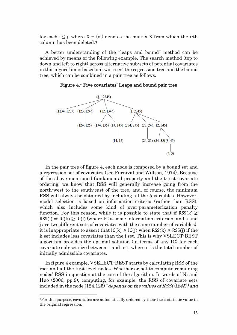
Figure 4.- Five covariates’ Leaps and bound pair tree
In the pair tree of figure 4, each node is composed by a bound set and
a regression set of covariates (see Furnival and Willson, 1974). Because
of the above mentioned fundamental property and the t-test covariate
ordering, we know that RSS will generally increase going from the
north-west to the south-east of the tree, and, of course, the minimum
RSS will always be obtained by including all the 5 variables. However,
model selection is based on information criteria (rather than RSS),
which also includes some kind of over-parameterization penalty
function. For this reason, while it is possible to state that if RSS(k) ≥RSS(j) ⇒ IC(k) ≥ IC(j) (where IC is some information criterion, and k and
j are two different sets of covariates with the same number of variables),
it is inappropriate to assert that IC(k) ≥ IC(j) when RSS(k) ≥ RSS(j) if the
k set includes less covariates than the j set. This is why VSLECT-BEST
algorithm provides the optimal solution (in terms of any IC) for each
covariate sub-set size between 1 and n-1, where n is the total number of
initially admissible covariates.
In figure 4 example, VSELECT-BEST starts by calculating RSS of the
root and all the first level nodes. Whether or not to compute remaining
nodes’ RSS in question at the core of the algorithm. In words of Ni and
Huo (2006, pp.9), computing, for example, the RSS of covariate sets
included in the node (124,125) “depends on the values of RSS({1245}) and
7For this purpose, covariates are automatically ordered by their t test statistic value in
the original regression.
14
RSS({123}). If RSS({123})≤RSS({1245}), because {124} and {125} are subsets of {1245}, we immediately have RSS({123})≤RSS({124}) and RSS({123}) ≤RSS({125}). Hence, there is no need to compute for RSS({124}) and RSS({125}). Otherwise, they should be computed. Similarly, whether or not to compute RSS({134}) and RSS({135}) (or RSS({13}) and RSS({145})) depends on three values: RSS({12}), RSS({1345}), and min(RSS({123}), RSS({124}), RSS({125})) (denoted as RSS(3)). Note that RSS(3)≤RSS({12}). There are three cases for those three values: a) If RSS({12})≤ RSS({1345}), then none of RSS({134}), RSS({135}), RSS({13}), or RSS({145}) needs to be calculated. b) If RSS(3)≤RSS({1345})<RSS({12}), then only RSS({13}) and RSS({145}) need to be calculated to update the minimum RSS with 2 covariates. c) If RSS({1345})<RSS(3), then all of the four RSS’s need to be calculated.”
Because of this search space reduction, the original “2n order” model
selection problem becomes a “2n/p order” problem (where 1/p is the
reduction success rate), without losing the in-sample accuracy of (more
time consuming) complete-exhaustive methods. As a result of this
property (ensuring in-sample optimality with a reduced search
universe), VSELECT-BEST overcomes the most important weakness of
heuristic methods and emerge as the best model selection alternative for
moderate-size problems (between 20 and 40 variables), in which in-
sample explanation and not out-of-sample forecasting is the main
objective.
However, Lindsey and Sheter (2010) package still faces three
important limitations: 1) The algorithm’s main property does not apply
for out-of-sample model selection problems (e.g. we cannot ensure that
RSSout(S1) ≥ RSSout(S2) if S1 ⊆ S2); 2) While more efficient than complete-
exhaustive methods, for large size problems the VSELECT-BEST
approach becomes unfeasible and very time consuming (because the
success reduction rate will not compensate the exponential increase of
the problem size with the number of potential covariates); and 3) Since
it has not been designed to deal with robustness analysis, it only keeps
best model results of each subset size (leaving aside many crucial
outcomes for comparison purposes).
3 The Global Search Regression (GSREG) procedure
Thirty years ago, Professor Alan J. Miller developed an interesting
comparison of alternative (heuristic and exhaustive) model selection
approaches to conclude that “an exhaustive search… is recommended when feasible… [and] that the best 10 or 20 subsets of each size, not just the best one, should be saved. The closeness of fit of these competitors gives an indication of the likely bias in least-squares regression coefficients” (Miller, 1984; pp. 408).

15
Previous proposition stylishly summarizes the underlying reasons to
develop GSREG, a STATA® code (inspired by Coen, Gomme and Kendall
(1969)’ original insights) that: 1) guarantees optimality even with out-
of-sample selection criteria; 2) allows residual testing for each
alternative; 3) retains VSELECT leaps-and-bound “shortcuts” for in-
sample selection criteria; and 4) provides (depending on user
specifications) a full-information dataset with outcome statistics for
every alternative model. These features make GSERG a valuable tool
for high-accuracy forecasting and parameter robustness comparisons.
In spite of the above documented increase in computational
capabilities, our complete-exhaustive algorithm is particularly
recommended for small-size (less than 30 variables) model selection
problems, where: 1) out-of-sample selection criteria will be used to select
the optimal choice; and/or 2) the main researcher objective is about
parameter stability across different model specifications.
However, its options are encompassing enough to transform GSREG
in a flexible device for many other alternative uses. In what follows, all
its features are presented in detail.
The gsreg command has two major stages. In the first one, it creates
a set of lists, wherein each list contains one of the possible sets of
dependent variables, and therefore, the full set of lists contains all
possible combinations of candidate covariates. In the second stage, the
command performs a regression for each of the lists previously created.
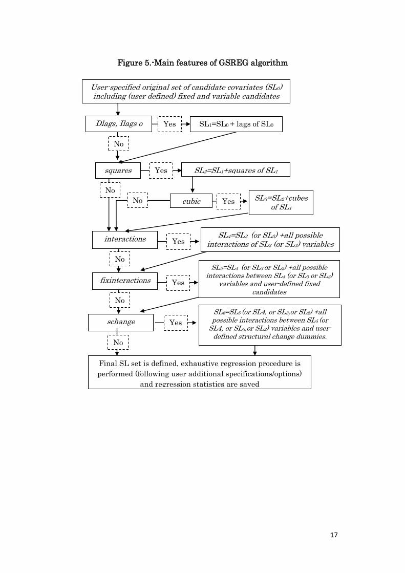
In the first stage the set of lists is determined according to the
following steps:
1) The algorithm determines an inventory containing the total set
of candidate variables, Lvc, according to the list of user-specified
original variables and the additional covariates to be included as
candidates if some of the options dlags, ilags orlags are
specified.
2) If the ncomb option is not specified, a first set of lists is created,
SL, taking all possible combinations without repetition of
candidate variables (which include all combinations taken from
1 up to the total number of variables in Lvc). Otherwise, SL is
created by taking all combinations without repetition of
candidate variables taken from integer1 to integer2 defined
inncomb option. So, SL={Lint!,.....,L int2} where each Li is a
particular subset of the set of candidate variables, Lvc. 3) If the squares option is specified, from each Li of point 2 an
additional list is created (SqLi), which includes every covariate
in Li plus all they squares. Then, the whole set of SqLi lists (SqL)
is added to the SL set. If the cubic option is additionally
16
specified, another group oflists(CubL) is created from the SqL set
by generating a CubLi list for each SqLi list, in which SqLi covariates are complemented by Li cubes. After that, the CubL
set is added to SL8.
4) If theinteractions option is specified, an additional IntLi list
is created from each Li, which includes all Li variables plus all
possible combinations without repetition of the interactions of
these variables. Then IntLi lists are added to SL.
5) By using the fixinteractions option, users are able to create
a FintLi new list from each Li, which not only includes all Li
variables but also all possible combinations without repetition of
the interactions between Li variables and fixvar variables (see
below).
6) If the schange option is specified, a new set of lists (SC) is
created from SL (already modified, if specified, by ilags,
dlags, ncomb, squares, cubic, interactions, and/or
fixinteractions) to test the existence of structural change in
every bivariate relationship, including all possible combinations
without repetition of the interactions between SL variables and
the user-defined variable of structural change (e.g a step or a
point dummy variable). Then, SC is added to SL.
In the second stage, GSERG exhaustively performs one regression per
SL list, saving coefficients and different (default and user-defined)
statistics in a Stata .dbf file. More precisely, for each SL list GSREG
outcomes include:
a) Coefficients and t-statistics of each covariate.
b) Regression number (regression id), number of covariates and
number of observations.
c) Default additional statistics (adjusted r-squared, rmse), optional
additional statistics (such as residual test p-values, out-of-
sample rmse out, etc.), and other user-defined statistics that user
specifies in the cmdstat option.
The following scheme summarizes GSREG procedure:
8 Notice that this procedure dismisses all those lists (regressions) which include
squares of a certain variable but do not include the original variable (e.g. in levels),
thereby reducing the number of estimations to be performed. If users would like to
estimate the cases where a given variable appears only in quadratic terms, they should
simply include the square of that variable (or all variables he wants) as an independent
variable in the original Lvc set. Also notice that for the case of the cubic option, the
algorithm only generates lists with the cubes of the variables for which the square
was included. Similar criteria were applied to the interaction, fixinteractions
and schange options explained in the following sections.
17
Figure 5.-Main features of GSREG algorithm
No
Yes
No
SL1=SL0 + lags of SL0
squares
SL4=SL2 (or SL3) +all possible interactions of SL2 (or SL3) variables
cubic SL3=SL2+cubes of SL1
interactions
SL5=SL4 (or SL3 or SL2) +all possible interactions between SL4 (or SL3 or SL2)
variables and user-defined fixed candidates
fixinteractions
SL6=SL5 (or SL4, or SL3,or SL2) +all possible interactions between SL5 (or
SL4, or SL3,or SL2) variables and user-defined structural change dummies.
schange
Final SL set is defined, exhaustive regression procedure is
performed (following user additional specifications/options)
and regression statistics are saved
SL2=SL1+squares of SL1
Dlags, Ilags o
lags
User-specified original set of candidate covariates (SL0) including (user defined) fixed and variable candidates
Yes
No
Yes
Yes
No
Yes
No
Yes
No
18
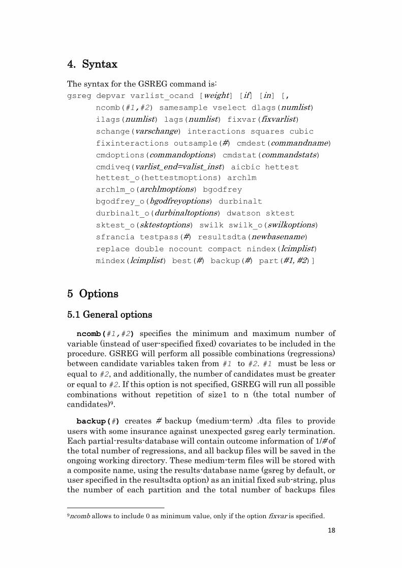
4. Syntax
The syntax for the GSREG command is:
gsreg depvar varlist_ocand [weight] [if] [in] [,
ncomb(#1,#2) samesample vselect dlags(numlist)
ilags(numlist) lags(numlist) fixvar(fixvarlist)
schange(varschange) interactions squares cubic
fixinteractions outsample(#) cmdest(commandname)
cmdoptions(commandoptions) cmdstat(commandstats)
cmdiveq(varlist_end=valist_inst) aicbic hettest
hettest_o(hettestmoptions) archlm
archlm_o(archlmoptions) bgodfrey
bgodfrey_o(bgodfreyoptions) durbinalt
durbinalt_o(durbinaltoptions) dwatson sktest
sktest_o(sktestoptions) swilk swilk_o(swilkoptions)
sfrancia testpass(#) resultsdta(newbasename)
replace double nocount compact nindex(lcimplist)
mindex(lcimplist) best(#) backup(#) part(#1, #2)]
5 Options
5.1 General options
ncomb(#1,#2) specifies the minimum and maximum number of
variable (instead of user-specified fixed) covariates to be included in the
procedure. GSREG will perform all possible combinations (regressions)
between candidate variables taken from #1 to #2. #1 must be less or
equal to #2, and additionally, the number of candidates must be greater
or equal to #2. If this option is not specified, GSREG will run all possible
combinations without repetition of size1 to n (the total number of
candidates)9.
backup(#) creates # backup (medium-term) .dta files to provide
users with some insurance against unexpected gsreg early termination.
Each partial-results-database will contain outcome information of 1/# of
the total number of regressions, and all backup files will be saved in the
ongoing working directory. These medium-term files will be stored with
a composite name, using the results-database name (gsreg by default, or
user specified in the resultsdta option) as an initial fixed sub-string, plus
the number of each partition and the total number of backups files
9ncomb allows to include 0 as minimum value, only if the option fixvar is specified.
19
specified in # (eg. gsreg_part_1_of_4.dta; gsreg_part_2_of_4.dta;
gsreg_part_3_of_4.dta; and gsreg_part_4_of_4.dta). All these files will be
deleted at the end of a successful gsreg execution (e.g. without any
unexpected early termination), because they will be replaced by a unique
total-results-database. If the number of total regressions to be
performed is lower than #, the number backup partitions will be equal
to the former. See Examples of using backup and part options.
part(#1,#2) allows users to simplify external parallelization
strategies by running in each (of potentially many parallel) Stata
instance only a user-specified share of the total number of regressions to
be estimated. Among the arguments of this option, the second integer
identifies the number of partitions that will be used to divide the SL set
(see section 3), and also defines the number of regressions of each
partition, which is about 1/#2 of the total number of regressions. In turn,
the first integer is used to select which-one of these partitions must be
used by GSREG in each Stata instance (e.g. part(1,3), part(2,3), and
part(3,3) could be combined –using only one of these options per Stata
instance- in three parallel Stata instances running gsreg on the same
SL set). If the number of total regressions to be performed is lower than
#2, the number part partitions will be equal to the former. See Examples
of using backup and part options
samesample makes all regressions to be performed over the same
sample of observations, defined as the largest common sample. By
default, GSREG performs each regression with the maximum number of
observations available for the covariate subset used in each particular
case.
vselect runs the command vselect (for vselect “best”
option)developed by Charles Lindsey and Simon Sheather (2010, which
has to be previously installed) to obtain the best n regressions (one for
each maximum number of covariates included: e.g. the best one
covariate model, the best two-covariates model and so on) in terms of in-
sample RMSE. When specifying vselect, the only additional option
that can be specified is the fixvar option.
5.2 Lag structure options
dlags(numlist>0 integer)allows to include dependent variable lags
(depvar) among candidate covariates.
dlags(#)adds among candidates the # dependent variable lag.
tsset must be specified when using this option.
dlags(#1/#2) adds among candidates all dependent variable lags
from #1 to #2 considering one-unit intervals.
20
dlags(#1 #2 #3) adds among candidates the #1, the #2, and the #3
dependent variable lags.
dlags(#1 (#d) #2) adds among candidates all dependent variable
lags from #1 to #2 considering #d unit intervals.
dlags(#1 #2 #3 … #4 (#d) #5)adds among candidates dependent
variable lags #1,#2, and #3, and additionally all dependent variable lags
from #4 to #5 considering #d unit intervals.
ilags(numlist>0 integer)10,11 allows including independent variable
lags among original candidates. The syntax is flexible and identical to
that used indlags.
lags(numlist>0 integer) allows to jointly include dependent and
independent variable lags among original candidates. It replaces dlags
and ilags when the argument is identical. tsset must be specified
when using this option. lags must not be specified together with dlags
or ilags.
5.3 Fixed variable options
fixvar(varlist_fix) allows to specify a subset of covariates which
must be included in all regressions. Variables defined in varlist_fix must
not be included among the standard candidates (varlist_ocand).
5.4 Options for transformations and interactions
schange(varschange) tests structural change of slops (using dummy
varschange as interaction with all candidates) or dependent variable
levels (alternatively allowing varschange to interact with the intercept).
Interactions of varschange with any candidate will only be included if
this candidate is in the equation. varschange must not be included
among original candidates (varlist_ocand) because it will only be used
for structural change.
interactions includes additional covariate candidates to evaluate
all possible interactions without repetition among candidates.
Interactions between any two candidates will only be allowed if both of
10 Using ilags and dlags options is equivalent to generate independent and dependent
variables lags (respectively) before using GSREG and include them among original
candidates. 11 Users looking for different candidate lag structures for each covariate should not
specify the option ilags but, instead, create desired candidate lag structures before
using GSREG and include them in the whole set of original candidates.
21
them are in the equation. When used together with schange, the
structural change of interactions will only be used if these interactions
are included in the estimated specification.
squares adds the squares of each variable in varlist_ocand as new
candidates. Each square will only be accepted as a regression covariate
if its level (original variable) is present in the equation. Similarly, when
used together with schange, the structural change of the squares will
only be allowed if these squares are in the equation.
cubic is similar to squares. It includes cubes of each variable in
varlist_ocand as new candidates. These cubes will only be accepted as
covariates if level and squares of the same variable are also included in
the equation. As for squares, when used together with schange, the
structural change of the cubes will only be allowed if these cubes are also
in the equation.
fixinteractions is similar to interactions, but it only includes
as additional candidates all possible interactions without repetition
among each standard candidate and each fixed variable in varlist_fix.
5.5 Options for time series and panel data forecasts
outsample(#)is used in time series and panel models. It splits the
sample into two. The first sub-sample is used for regression purposes
and the second one is applied to evaluate forecast accuracy.
outsample(#)leaves the last #periods to make forecasts (so that
regressions are performed over the first T-# periods – where T is the
total number of available time series observations). When this option is
specified, GSREG calculates the rmse_in (in sample root mean square error) between period 1 and N-#, and rmse_out (out sample root mean square error) between period N-# and N. tsset must be specified when
using this option.
5.6 Regressions command options
cmdest(commandname)12 allows choosing the regression command
to be used. If the option is not specified, commandname default is
regress. This option allows using regress, xtreg, probit, logit,
areg, qreg and plreg, but it additionally accept any regression
command that respects the syntax of regress and saves results (matrices
12Not all GSREG options can be used in any regression command; and for regression
commands with required (compulsory) options, it will be necessary to specify them in cmdoptions.
22
e(b) and e(V)) in the same way. ivregress is also accepted but
complementarily using option cmdiveq(varlist_end =
varlist_inst). See Examples of using cmdest, cmdoptions,
cmdstat and cmdiveq.
cmdoptions(commandoptions)allows addingsu pported (by
commandname) additional options for each regression
cmdstat(commandstats)enables GSREG(which automatically
saves the number of observations –obs., the number of covariates -nvar-
, the adjusted R2 -r_sqr_a- and the root mean square error -rmse_in)
to save additional regression statistics (included as scalars in e())
specified in commandstats.
cmdiveq(varlist_end = varlist_inst)is a special GSREG
option for ivreg estimations, which can be used to specify varlists of
endogenous variables (varlist_end) and instruments
(varlist_inst). When using this option, cmdest(ivregress 2sls),
cmdest(ivregress liml) or cmdest(ivregress gmm) must also
be specified, and the endogenous variables must also be included in
varlist_fix or in varlist_ocand. See Examples of using cmdest,
cmdoptions, cmdstat and cmdiveq.
5.7 Post-estimation options
5.7.1 Information criteria
aicbic calculates estat ic after each regression to obtain Akaike
(aic) and Bayesian information criteria (bic)
5.7.2 Heteroscedasticitytests
hettest calculates default estat hettest after each regression
and saves p-values.
hettest_o(hettestmoptions) allows adding options to hettest.
archlm runs default estat archlm after each regression and saves
p-values. tsset must be specified when using this option.
archlm_o(archlmoptions)allows adding options to archlm.
5.7.3 Serial autocorrelation tests
23
bgodfrey computes default estat bgodfrey after each regression
and saves p-values. tsset must be specified when using this option.
bgodfrey_o(bgodfreyoptions) allows adding options to bgodfrey.
durbinalt calculates estat durbinalt after each regression and
saves the p-values. tsset must be specified when using this option.
durbinalt_o(durbinaltoptions)allows adding options to durbinalt.
dwatson runs estat dwatson after each regression and saves the
Durbin-Watson statistic. tsset must be specified when using this
option.
5.7.4 Normality tests of residuals
sktest computes sktest after each regression and saves the p-
value of the joint probability of skewness and kurtosis for normality.
tsset must be specified when using this option.
sktest_o(sktestoptions) allows adding options to sktest.
swilk calculates swilk after each regression and saves the p-value
of the Shapiro-Wilk normality test. tsset must be specified when using
this option.
swilk_o(swilkoptions) allows adding options to swilk.
sfrancia runs sfrancia after each regression and saves the p-
value of the Shapiro-Francia normality test. tsset must be specified
when using this option.
testpass(#) allows a reduction of the outcome database size by
saving only those regression results that fulfilled all user-specified
residual tests (at a # significance level).
5.5 Output options
resultsdta(newbasename) allows results database name to be
user defined in newbasename. By default, the name will be gsreg.dta.
replace replaces the results database if it is already created (with
the same name) in the ongoing working directory.
double forces results to be created and saved in double format, that
is, with double precision.
24
nocount hides from the screen the number of regression which is
being estimated. If this option is not specified, GSERG will show for each
regression its number (used for identification purposes) and the total
number of regressions to be estimated.
compact reduces the results database size by deleting all coefficients
and t statistics. In their place, GSREG creates a string variable called
regressors that describes which candidate variables are included in each
regression. This variable takes value “1” in position # if the candidate
variable with position # is included in the equation, and it takes value
“.” if it is not. Variable positions are kept in a small database called
newbasename_labels.dta (where newbasename is the results database
user defined name).
nindex(lcimplist) allows specifying an index of normalized accuracy
–nindex-. Regressions will be ordered from highest to lowest nindex in
the results database, and the best regression according to nindex will
be shown on screen at the end of the GSREG execution. If not specified,
nindex will be based on the adjusted R-squared (r_sqr_a). User choices
about goodness-of-fit or forecast accuracy criteria on nindex can flexibly
be specified in lcimplist. By means of user-selected weights and ranking
variables, lcimplist allows complex arguments to create multinomial
ordering criteria. Any results-database variable can be used in the
lcimplist argument as a ranking variable (e.gr_sqr_a, rmse-in, rmse-out,
aic, bic, etc.), but it must be preceded by a user-defined real number
weight as in the following example: nindex(0.3 r_sqr_a -0.3 aic -0.4 bic).
It should be noticed that each variable included in lcimplist is
normalized using the whole sample average (across of all regressions) of
the same variable.
mindex(lcimplist)and best(#)options must be specified together.
mindex generates a normalized ranking index like nindex, and has the
same syntax (see nindex option), but the normalization of its
arguments is developed using averages obtained from the best# +1regressions. Therefore, mindex is updated with each additional
regression and only the best (in terms of lcimplist)# regressions results
are saved. The joint use of mindex and best options can strongly reduce
database size (and RAM requirements) making feasible larger model
selection problems. However, as mindex must be re-calculated with
every regression, GSERG could run slower than using nindex
(particularly for small model selection problems).
25
6 Examples
GSREG can be used for many purposes. In this chapter, we introduce
three straightforward illustrations of different GSREG applications. For
brevity matters, option specifications are not fully discussed here.
Interested users will find a much in deep explanation (and option
examples) in the GSREG help file.
In the first example, we use artificial data to see how GSREG can be
useful to obtain the best model in terms of in-sample goodness-of-fit,
provided that regression residuals fulfill some desirable property.
The second example shows that a complete search method (as
GSERG) could be indispensable if out-of-sample accuracy is the main
user concern for model selection.
Our third example illustrates another valuable GSERG application:
parameter stability analysis (across different control variable model
structures).
6.1 Model selection and residual tests
The Leaps and Bound efficient model selection methodology
(introduced in Stata by the vselect command) has two salient
characteristics: 1) by using an exhaustive search method (see section 2
and sub-section 2.3), it ensures optimality in terms of any in-sample
model selection criterion; and 2) the embedded Furnival and Wilson
(1974) efficient algorithm allows exhaustive search to be performed over
a larger number of covariates than that feasible for complete search
algorithms.
However, the best model (or models) in terms of some in-sample
information criterion do not necessarily fulfill required residual
properties (something left aside by veselect and other model selection
Stata commands like stepwise). The following very small and clear
example shows why GSREG-like algorithms can be essential to deal
with this problem.
Suppose we wish to obtain the best model to explain𝑦, using some
combination of two covariates, 𝑥 and𝑧, and assuming the following data
generating process (DGP):
𝑦𝑡 = 𝛽0 + 𝛽1𝑡𝑥1𝑡 + 𝛽2𝑡𝑧𝑡+𝑢𝑡
𝑡 = 1, … ,1000
𝛽0 = 1
26
𝛽1𝑡 = 0.9si t < 600 , 𝛽1𝑡 = 0si t ≥ 600
𝛽2𝑡 = 0si t ≤ 800 , 𝛽2𝑡 = 0.1 si t > 800
𝑧~𝑈[0,1],
𝑥~𝑈[0,2] si t < 600, 𝑥~𝑈(0,2.4)si t ≥ 600
𝑢~𝑁(0,1)
By construction, 𝑥covariate has a higher explanatory power than 𝑧,
but tends to generate heteroscedasticity problems.
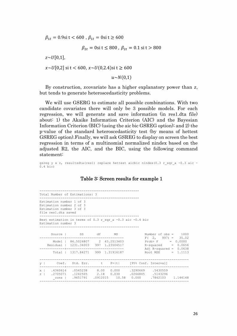
We will use GSERG to estimate all possible combinations. With two
candidate covariates there will only be 3 possible models. For each
regression, we will generate and save information (in res1.dta file)
about: 1) the Akaike Information Criterion (AIC) and the Bayesian
Information Criterion (BIC) (using the aic bic GSREG option); and 2) the
p-value of the standard heteroscedasticity test (by means of hettest
GSREG option).Finally, we will ask GSREG to display on screen the best
regression in terms of a multinomial normalized nindex based on the
adjusted R2, the AIC, and the BIC, using the following command
statement:
gsreg y x z, resultsdta(res1) replace hettest aicbic nindex(0.3 r_sqr_a -0.3 aic -
0.4 bic)
Table 3: Screen results for example 1
----------------------------------------------------
Total Number of Estimations: 3
----------------------------------------------------
Estimation number 1 of 3
Estimation number 2 of 3
Estimation number 3 of 3
file res1.dta saved
----------------------------------------------------
Best estimation in terms of 0.3 r_sqr_a -0.3 aic -0.4 bic
Estimation number 3
----------------------------------------------------
Source | SS df MS Number of obs = 1000
-------------+------------------------------ F( 2, 997) = 35.02
Model | 86.5026807 2 43.2513403 Prob> F = 0.0000
Residual | 1231.34003 997 1.23504517 R-squared = 0.0656
-------------+------------------------------ Adj R-squared = 0.0638
Total | 1317.84271 999 1.31916187 Root MSE = 1.1113
------------------------------------------------------------------------------
y | Coef. Std. Err. t P>|t| [95% Conf. Interval]
-------------+----------------------------------------------------------------
x | .4360614 .0545238 8.00 0.000 .3290669 .5430559
z | .2705071 .1242505 2.18 0.030 .0266845 .5143296
_cons | .9651791 .0912015 10.58 0.000 .7862103 1.144148
------------------------------------------------------------------------------
27
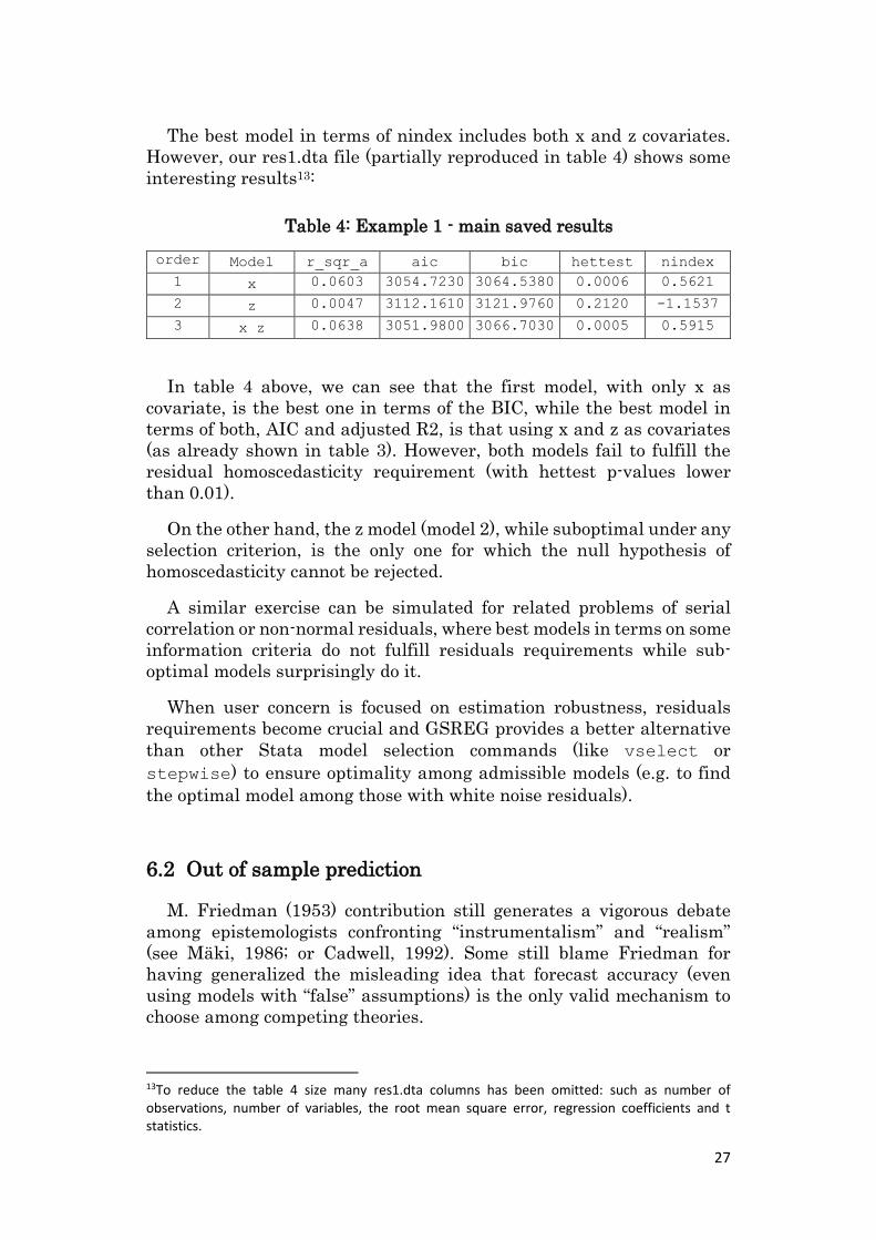
The best model in terms of nindex includes both x and z covariates.
However, our res1.dta file (partially reproduced in table 4) shows some
interesting results13:
Table 4: Example 1 - main saved results
order Model r_sqr_a aic bic hettest nindex
1 x 0.0603 3054.7230 3064.5380 0.0006 0.5621
2 z 0.0047 3112.1610 3121.9760 0.2120 -1.1537
3 x z 0.0638 3051.9800 3066.7030 0.0005 0.5915
In table 4 above, we can see that the first model, with only x as
covariate, is the best one in terms of the BIC, while the best model in
terms of both, AIC and adjusted R2, is that using x and z as covariates
(as already shown in table 3). However, both models fail to fulfill the
residual homoscedasticity requirement (with hettest p-values lower
than 0.01).
On the other hand, the z model (model 2), while suboptimal under any
selection criterion, is the only one for which the null hypothesis of
homoscedasticity cannot be rejected.
A similar exercise can be simulated for related problems of serial
correlation or non-normal residuals, where best models in terms on some
information criteria do not fulfill residuals requirements while sub-
optimal models surprisingly do it.
When user concern is focused on estimation robustness, residuals
requirements become crucial and GSREG provides a better alternative
than other Stata model selection commands (like vselect or
stepwise) to ensure optimality among admissible models (e.g. to find
the optimal model among those with white noise residuals).
6.2 Out of sample prediction
M. Friedman (1953) contribution still generates a vigorous debate
among epistemologists confronting “instrumentalism” and “realism”
(see Mäki, 1986; or Cadwell, 1992). Some still blame Friedman for
having generalized the misleading idea that forecast accuracy (even
using models with “false” assumptions) is the only valid mechanism to
choose among competing theories.
13To reduce the table 4 size many res1.dta columns has been omitted: such as number of observations, number of variables, the root mean square error, regression coefficients and t statistics.
28
In econometrics, there is some parallelism with the “measurement
without theory” debate associated to Koopmans (1947) almost 70 year
ago (and reviewed by Hendry and Morgan, 1995) and more recent
methodological discussions about in-sample vs out-of-sample model
selection mechanisms, where renowned econometricians like Ashley,
Granger and Schmalensee (1980) assert that “a sound and natural
approach” to testing predictive ability “must rely primarily on the out-
of-sample forecasting performance” (p. 1149).
It is not surprising that many colleagues increasingly consider to
overcome this last controversy by examining both in-sample and out-of-
sample model outcomes.
In this context, GSREG is able to ensure in-sample as well as out-of-
sample model selection optimality, reducing user concerns about
structural breaks in multivariate relationships.
To illustrate this point, suppose that we wish to get the best model of
𝑦 (in terms of some out-of-sample criterion) based on 𝑥 and/or 𝑧, with 100
time series observations (using the last 20 to out-of-sample model
evaluation), and assuming the following data generating process:
𝑦𝑡 = 𝛽0 + 𝛽1𝑥1𝑡 + 𝛽2𝑡𝑧𝑡+𝑢𝑡
𝛽0 = 1
𝛽1 = 1
𝛽2𝑡 = 1si t ≤ 70
𝛽2𝑡 = 0 si t > 70
𝑥, 𝑧, 𝑢~𝑁(0,1)
By construction, both covariates have a high in-sample explanatory
power, but 𝑧 becomes non significant for out-of-sample evaluation
purposes.
If the structural change is unknown (and therefore disregarded) and
we don’t use GSREG to evaluate forecast accuracy, the best “y”
representation will obviously include x and z as covariates.
On the contrary, users concerned about the dangerous effects of
potential structural breaks will exploit some database sub-sample to
check parameter stability (e.g. the last 20 observations) and use GSREG
to examine both explanatory power and forecast accuracy of each
alternative model. For this example, the simplest sentence could be:
gsreg y x z, outsample(20) replace
29
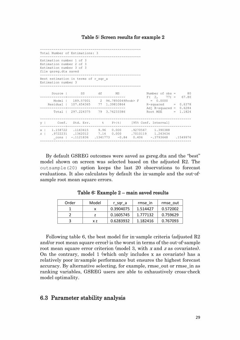
Table 5: Screen results for example 2
----------------------------------------------------
Total Number of Estimations: 3
----------------------------------------------------
Estimation number 1 of 3
Estimation number 2 of 3
Estimation number 3 of 3
file gsreg.dta saved
----------------------------------------------------
Best estimation in terms of r_sqr_a
Estimation number 3
----------------------------------------------------
Source | SS df MS Number of obs = 80
-------------+------------------------------ F( 2, 77) = 67.80
Model | 189.57001 2 94.7850049Prob> F = 0.0000
Residual | 107.654365 77 1.39810864 R-squared = 0.6378
-------------+------------------------------ Adj R-squared = 0.6284
Total | 297.224375 79 3.76233386 Root MSE = 1.1824
------------------------------------------------------------------------------
y | Coef. Std. Err. t P>|t| [95% Conf. Interval]
-------------+----------------------------------------------------------------
x | 1.158722 .1163415 9.96 0.000 .9270567 1.390388
z | .9722231 .1362012 7.14 0.000 .7010119 1.243434
_cons | -.1121836 .1341773 -0.84 0.406 -.3793648 .1549976
------------------------------------------------------------------------------
By default GSREG outcomes were saved as gsreg.dta and the “best”
model shown on screen was selected based on the adjusted R2. The
outsample(20) option keeps the last 20 observations to forecast
evaluations. It also calculates by default the in-sample and the out-of-
sample root mean square errors.
Table 6: Example 2 – main saved results
Order Model r_sqr_a rmse_in rmse_out
1 x 0.3904075 1.514427 0.572002
2 z 0.1605745 1.777132 0.759629
3 x z 0.6283932 1.182416 0.767093
Following table 6, the best model for in-sample criteria (adjusted R2
and/or root mean square error) is the worst in terms of the out-of-sample
root mean square error criterion (model 3, with x and z as covariates).
On the contrary, model 1 (which only includes x as covariate) has a
relatively poor in-sample performance but ensures the highest forecast
accuracy. By alternative selecting, for example, rmse_out or rmse_in as
ranking variables, GSREG users are able to exhaustively cross-check
model optimality.
6.3 Parameter stability analysis
30
By generating a database with exhaustive information about all
regression alternatives, GSERG is a unique tool for parameter stability
analysis.
In this example, we will use the crisis_fr database of Gluzmann and
Guzman (2011) (containing information on financial crisis, financial
reforms and a set of controls for 89 countries along the period 1973-2005)
to evaluate interest parameter stability under alternative control
variable structures.
As a first step, we run a pooled-data (for Latin American countries
Emerging Asia and transition economies) linear regression of the
probability of future financial crisis over the next 5 years (fc5), on a
financial reform index (ifr) and its recent change (d_ifr).
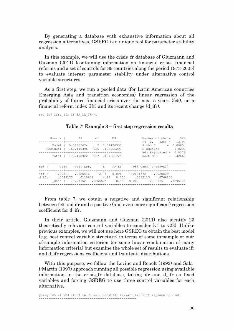
reg fc5 ifrd_ifr if EA_LA_TR==1
Table 7: Example 3 – first step regression results
Source | SS df MS Number of obs = 928
-------------+------------------------------ F( 2, 925) = 13.97
Model | 5.08852674 2 2.54426337 Prob> F = 0.0000
Residual | 168.410396 925 .182065293 R-squared = 0.0293
-------------+------------------------------ Adj R-squared = 0.0272
Total | 173.498922 927 .187161729 Root MSE = .42669
------------------------------------------------------------------------------
fc5 | Coef. Std. Err. t P>|t| [95% Conf. Interval]
-------------+----------------------------------------------------------------
ifr | -.00711 .0025616 -2.78 0.006 -.0121372 -.0020829
d_ifr | .0549173 .0110602 4.97 0.000 .0332113 .0766233
_cons | .2793652 .0255525 10.93 0.000 .2292176 .3295128
------------------------------------------------------------------------------
From table 7, we obtain a negative and significant relationship
between fc5 and ifr and a positive (and even more significant) regression
coefficient for d_ifr.
In their article, Gluzmann and Guzman (2011) also identify 23
theoretically relevant control variables to consider (v1 to v23). Unlike
previous examples, we will not use here GSREG to obtain the best model
(e.g. best control variable structure) in terms of some in-sample or out-
of-sample information criterion (or some linear combination of many
information criteria) but examine the whole set of results to evaluate ifr
and d_ifr regressions coefficient and t-statistic distributions.
With this purpose, we follow the Levine and Renelt (1992) and Sala-
i-Martin (1997) approach running all possible regression using available
information in the crisis_fr database, taking ifr and d_ifr as fixed
variables and forcing GSREG to use three control variables for each
alternative.
gsreg fc5 v1-v23 if EA_LA_TR ==1, ncomb(3) fixvar(ifrd_ifr) replace nocount
----------------------------------------------------
31
Total Number of Estimations: 1771
----------------------------------------------------
file gsreg.dta saved
GSERG execution time takes less than a minute using STATA/MP
12.1 for windows (64b) in a laptop with a Intel i7-3520m processor and
4Gb of DDR3 RAM memory. The fixvar(.) option ensures that ifr and
d_ifr will be used as covariates in all regressions. The ncomb(3) option
reduces the search space to all possible combinations (without
repetition) of 23 control variables taken 3 at time.
Main command outcomes can easily be described by means of the
following kernel density plot.
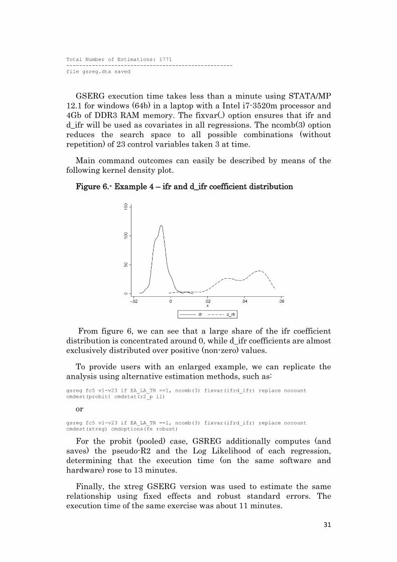
Figure 6.- Example 4 – ifr and d_ifr coefficient distribution
From figure 6, we can see that a large share of the ifr coefficient
distribution is concentrated around 0, while d_ifr coefficients are almost
exclusively distributed over positive (non-zero) values.
To provide users with an enlarged example, we can replicate the
analysis using alternative estimation methods, such as:
gsreg fc5 v1-v23 if EA_LA_TR ==1, ncomb(3) fixvar(ifrd_ifr) replace nocount
cmdest(probit) cmdstat(r2_p ll)
or
gsreg fc5 v1-v23 if EA_LA_TR ==1, ncomb(3) fixvar(ifrd_ifr) replace nocount
cmdest(xtreg) cmdoptions(fe robust)
For the probit (pooled) case, GSREG additionally computes (and
saves) the pseudo-R2 and the Log Likelihood of each regression,
determining that the execution time (on the same software and
hardware) rose to 13 minutes.
Finally, the xtreg GSERG version was used to estimate the same
relationship using fixed effects and robust standard errors. The
execution time of the same exercise was about 11 minutes.

32
7 Saved results
The GSREG command creates a .dtafile with outcome information for
all estimated alternatives. By default it includes the following columns
for each regression:
1) regression id (variable order),
2) covariate regression coefficients (named v_1_b, v_2_b… , etc., and
labeled with the full covariate name plus the word “coeff.”),
3) coefficient t-statistics (namedv_1_t, v_2_t…, etc., and labeled with
the full covariate name plus the word “tstat.”),
4) number of observations (variable obs),
5) number of covariates(nvar),
6) adjusted R2 (r_sqr_a),
7) in-sample root mean square error (rmse_in),
8) normalized linear combination of user selected (and weighted)
model selection criteria (as nindexor mindex if this option is specified)
9) additional user specified statistics (if the cmdstat option is
specified),
10) out-of-sample root mean square error (if outsample option is
specified), and
11) residual test statistics (if specified).
When compact option is specified, regression coefficients and t-
statistics are omitted and replaced by a unique summary string variable
as described in section 5.5.
In addition, GSERG shows on screen the best regression in terms of
the user specified nindex or mindex (or the adjusted R2 if these options
are not specified). Therefore, all this “best model” results are also saved
in memory (as scalars, macros, matrices and functions).
8 Acknowledgments
This work was supported by the Argentine National Agency for
Scientific and Technological Promotion [PICT 2010/2719]; and the
Argentine National Council of Scientific and Technical Research.
33
The authors wish to thank Amalia Torija-Zane, Diego Herrero,
Fernando Toledo and Martín Guzmán, who gave valuable suggestion
that has helped us to improve the quality of GSREG.
9 References
Ashley, R., C.W.J. Granger, and R. Schmalensee (1980). Advertising
and Aggregate Consumption: An Analysis of Causality. Econometrica
48, 1149-67.
Berk, K. N. (1978). Comparing subset regression procedures.
Technometrics, 20, 1–6.
Box, G. E. P., and Newbold, P. (1971). Some comments on a paper of
Coen, Gomme, and Kendall. Journal of the Royal Statistical Society, A,
134, 229–240.
Breiman, L. (1995). Better subset regression using the nonnegative
garrote. Technometrics, 37, 373–384.
Caldwell, B. (1992). Friedman’s methodological instrumentalism: A
Modification, Research in the History of Economic Thought and Methodology, 10, 119-128
Castle, J. (2006). Empirical modeling and model selection for
forecasting inflation in a non-stationary world. Ph.D. Thesis, Nuffield
College University of Oxford.
Coen, P. G., Gomme, E. D., and Kendall, M. G. (1969).Lagged
relationships in economic forecasting. Journal of the Royal Statistical Society A, 132, 133–163.
Davidson, J. E. H., and Hendry, D. F. (1981).Interpreting econometric
evidence: Consumers’ expenditure in the UK. European Economic Review, 16, 177–192. Reprinted in Hendry, D. F. (1993), Econometrics:
Alchemy or Science? Oxford: Blackwell Publishers.
Derksen, S. and H. J. Keselman (1992). Backward, forward and
stepwise automated subset selection algorithms: frequency of obtaining
authentic and noise variables. British Journal of Mathematical and Statistical Psychology 45:265–282.
Doornik, J. A. (2008) Autometrics, in J. L. Castle and N. Shephard
(eds.) The Methodology and Practice of Econometrics: A Festschrift in
Honour of David F. Hendry, Oxford University Press, Oxford.
Draper, N. and Smith, H. (1966). Applied regression analysis. New
York: Willey.
34
Duarte Silva, P. (2009). Exact and heuristic algorithms for variable
selection: extended leaps and bounds. Working Paper Nº 01/2009
Universidade Católica Portuguesa, Facultade de Economia e Gestão,
Porto, Portugal.
Efron, B., Hastie, T., Johnstone, I. and Tibshirani, R. (2004). Least
angle regression. Annals of Statistics 32(2), 407-499.
Efroymson, M. A. (1960). Multiple regression analysis. In Ralston, A.,
and Wilf, H. S. (eds.), Mathematical Methods for Digital Computers, pp.
191–203. New York: John Wiley & Sons
Forrest, S. and Mitchell, M. (1991). The Performance of Genetic
Algorithms on Walsh Polynomials: Some Anomalous Results and their
Explanation. Proc. 4th Intl. Conf. on Genetic Algorithms, La Jolla, CA:
Morgan Kaufmann.
Friedman, M. (1953). The methodology of positive economics, In:
Essays in Positive Economics, ed. M. Friedman, pp. 1-43, Chicago:
Chicago University Press
Frisch, R. (1934). Statistical Confluence Analysis by means of Complete Regression Systems. Oslo: University Institute of Economics.
Furnival, G. M., and R. W. Wilson.(1974). Regression by leaps and
bounds.Technometrics 16: 499–511.
Gatu, C. and Kontoghiorghes, E. J. (2006). Branch-and-bound
algorithms for computing the best subset regression models. Journal of Computational and Graphical Statistics, 15, 139–156
Gilbert, C. L. (1986). Professor Hendry’s econometric methodology.
Oxford Bulletin of Economics and Statistics, 48, 283–307.
Gluzmann, P. and M. Guzman (2011). Reformas financieras e
inestabilidad financiera. Ensayos Económicos, BCRA, Volumen 1, N°
61-62, pp. 35-73.
Haavelmo, T. (1944). The probability approach in econometrics.
Econometrica, 12, (supplement),1–118.
Hendry, D. F. (1980). Econometrics: Alchemy or science? Economica,
47, 387–406. Reprinted in Hendry (1993), pp. 11–28, and Hendry (2000),
pp. 11–28
Hendry, D. F. (1995). Dynamic Econometrics. Oxford: Oxford
University Press.
Hendry, D. F., and Morgan, M. S. (eds.)(1995).The Foundations of Econometric Analysis. Cambridge: Cambridge University Press.
35
Herwartz, H. (2007). A note on model selection in (time series)
regression models – General-to-Specific or Specific-to-General? Working
Paper 2007/09. Department of Economics, Christian-Albrechts-
Univesitat Kiel.
Hoover, K.D. (2006). The Methodology of Econometrics. In: New Palgrave Handbook of Econometrics, ed. by T.C. Mills and K. Patterson,
vol. 1: 61-87, Macmillan: London.
Koopmans, T. C. (1947). Measurement without theory. Review of Economics and Statistics, 29,161–179.
Krolzig, H.M. and D.F. Hendry (2001). Computer automation of
general-to-specific model selection procedures. Journal of Economic Dynamics & Control 25: 831-866.
Leamer, E. E. (1978). Specification Searches: Ad Hoc Inference with Non-Experimental Data. New York: John Wiley & Sons.
Levine, R. and Renelt, D. (1992).A sensitivity analysis of cross-
country growth regressions, American Economic Review, Vol. 82, pp.
942–963.
Lindsey C. and S. Sheather (2010).Variable Selection in Linear
Regression. The Stata Journal, 10: 650–669.
Lovell, M. C. (1983). Data mining. Review of Economics and Statistics,
65, 1–12.
Mäki, U. (1986). Rhetoric at the expense of coherence: A
reinterpretation of Milton Friedman's methodology, Research in the History of Economic Thought and Methodology, 4, 127-143
Marinucci, M. (2008). Automatic prediction and model selection.
Ph.D. Thesis, Facultad de Ciencias Económicas y Empresariales,
Universidad Complutense de Madrid.
Miller, A. (1984). Selection of subsets of regression variables. Journal of the Royal Statistical Society, A, 147, part 3, 389-425.
Ni, X. and X. Huo (2005). Enhanced leaps-and-bounds method in
subset selections with additional optimality tests.
http://www.informs.org/content/download/55245/522655/file/enhanced%
2520leaps%2520and%2520bounds.pdf+&cd=1&hl=es&ct=clnk&gl=ar.
Pagan, A. R. (1987). Three econometric methodologies: a critical
appraisal. Journal of Economic Surveys, 1, 3–24.
Pérez-Amaral, T., Gallo, G. and White, H. (2003). A Flexible Tool for
Model Building: the Relevant Transformation of the Inputs Network
36
Approach (Retina). Oxford Bulletin of Economics and Statistics 65, 821-
838.
Sala-i-Martin, X. X. (1997). I have just run two million regressions,
American Economic Review, Vol. 87, pp. 178–183.
Tibshirani, R. (1996). Regression shrinkage and selection via the
LASSO. Journal of the Royal Statistical Society B, 58, 267–288.
About the authors
Demian Panigo is Ph.D. in Economics (EHESS-Paris) and Associate
Researcher at the Argentine National Council of Scientific and
Technological Research (CONICET). He is professor of Advanced
Macroeconomics at the National University of La Plata and the National
University of Moreno, both in Argentina.
Pablo Gluzmann is Ph.D. in Economics (UNLP-La Plata) and
Graduate Fellow at the Argentine National Council of Scientific and
Technological Research (CONICET). He is assistant professor of
Advanced Macroeconomics at the National University of La Plata,
Argentina.
Revised and improved versions of GSREG will become available in the
future on the CEIL-CONICET web page (http://www.ceil-piette.gov.ar/).
Please address any correspondence to Demian Panigo (dpanigo@ceil-
conicet.gov.ar).