Embed Size (px)
Citation preview
Federal Reserve Bank of Dallas Globalization and Monetary Policy Institute
Working Paper No. 33 http://www.dallasfed.org/assets/documents/institute/wpapers/2009/0033.pdf
Global Slack and Domestic Inflation Rates: A Structural Investigation
for G-7 Countries*
Fabio Milani University of California, Irvine
August 2009
Abstract Recent papers have argued that one implication of globalization is that domestic inflation rates may have now become more a function of “global”, rather than domestic, economic conditions, as postulated by closed-economy Phillips curves. This paper aims to assess the empirical importance of global output in determining domestic inflation rates by estimating a structural model for a sample of G-7 economies. The model can capture the potential effects of global output fluctuations on both the aggregate supply and the aggregate demand relations in the economy and it is estimated using full-information Bayesian methods. The empirical results reveal a significant effect of global output on aggregate demand in most countries. Through this channel, global economic conditions can indirectly affect inflation. The results, instead, do not seem to provide evidence in favor of altering domestic Phillips curves to include global slack as an additional driving variable for inflation. JEL codes: E31, E50, E52, E58, F41
* Fabio Milani, Department of Economics, 3151 Social Science Plaza, University of California, Irvine, CA, 92697-5100. 949-824-4519. [email protected]. The views in this paper are those of the author and do not necessarily reflect the views of the Federal Reserve Bank of Dallas or the Federal Reserve System.
1
1. Introduction
The degree of global integration in goods, factor, and financial markets has substantially
increased over the last two decades. This process of globalization is likely to have induced sig-
nificant changes in the behavior of macroeconomic variables in most countries. Among other
things, several observers have argued that globalization may have altered the dynamics of in-
flation. First, many have recognized that globalization may have been a contributing factor
in reducing inflation rates around the world, although the size of its effect is controversial.1
But others have offered the more radical argument that, in a globalized economy, the popular
closed-economy Phillips curves, which relate current inflation rates to expected inflation and
current domestic resource utilization, may no longer be an appropriate description of infla-
tion behavior. Borio and Filardo (2007), in fact, provide empirical evidence that shows how
measures of “global”, rather than domestic, economic conditions may have now become the
relevant measure of unused capacity that drives inflation. An ensuing paper by Ihrig et al.
(2007), however, finds that global output is unimportant following a similar empirical strategy.
The aim of this paper is to evaluate the empirical importance of global output as a driver of
domestic inflation rates. But, while empirical work in this area has focused on single-equation
regressions, this paper uses a structural model, derived from microfounded behavior by house-
holds and firms, and estimated using full-information techniques, to assess the relevance of
global measures of output in the sample of G-7 countries.
The use of a structural model is motivated by the need to disentangle the different channels
through which global slack can play a role in the economy. Single equation estimations may
have difficulties controlling for the effect of global output on domestic output, for the influence
of monetary policies, for the effect of expectations, and, at least in the case of the U.S., for the
possible endogeneity of measures of global output to U.S. business cycle developments. These
factors can all be taken into account in the general equilibrium estimation.
The paper adopts the model derived in Clarida, Galı, and Gertler (2002, hereafter CGG)
and Woodford (2007) to capture the potential effects of foreign output fluctuations on domes-
tic macroeconomic behavior. Foreign output affects both the aggregate supply and demand
relations in the economy. It affects domestic output through the assumption that consumers
1Several researchers (e.g., Rogoff, 2003, 2006, Ball, 2006), policymakers (e.g., Fisher, 2005, Kohn, 2006,Bernanke, 2007), and the business press (e.g., The Economist), have debated the hypothesis that globalizationhas led to lower worldwide inflation.
2
in the home country consume a bundle of domestically-produced and foreign-produced goods.
Foreign output can, therefore, affect inflation both indirectly, through its effect on aggregate
demand, and directly, through its effect on firms’ marginal costs and hence on the specification
of the Phillips curve. In a globally-integrated economy, in fact, the decisions of domestic firms
to change their prices depend not only on domestic factors, but also on foreign (or global)
factors.
The model is estimated using Bayesian methods on quarterly data for the United States,
Japan, Germany, France, the United Kingdom, Italy, and Canada. The sample begins in 1985,
to focus on the period in which the pace of globalization has accelerated (the starting date
follows the choices by Borio and Filardo, 2007, and Ihrig et al., 2007). The relevant global
slack measure for each country is calculated as the weighted average of the output gap series
of a large set of its main trading partners, where the weights are given by the magnitude of
the country’s trade with each partner as a fraction of its total trade.
The main objective in the empirical analysis will be to check whether global output is a
significant factor in the domestic supply and demand equations. By revealing the channels
through which global output can affect domestic variables, the estimates can also shed light on
the benefits of alternative monetary policies. If global output plays a large role, in fact, central
banks may consider actively monitoring and responding to global macroeconomic conditions.
Moreover, as shown by CGG (2002), if strong spillovers from foreign output to domestic mar-
ginal costs and inflation rates exist, there will be non-trivial gains from international monetary
policy coordination.
The estimates reveal that measures of global slack have a sizeable influence on aggregate
demand in most countries. The empirical results, however, do not provide much support for
the relevance of a direct channel through which foreign output affects domestic inflation rates
by entering as an additional driving variable in the Phillips curve. The estimated sensitivities
of inflation to foreign output gaps are often negative and typically close to zero.
The best-fitting specifications for all countries, in fact, are those that include an effect of
global output on domestic output, but not a direct effect on domestic inflation. There is,
however, some uncertainty about the role of global slack in the Phillips curves for Italy and
France. In these cases, the specifications with and without global slack in the Phillips curve
are both assigned significant posterior probabilities.
3
Overall, mainly through the effect on domestic demand, global output can still affect do-
mestic inflation rates. From the variance decomposition, shocks to global conditions account
for a non-negligible share of output fluctuations in France, Germany, Canada, Italy, and the
U.K., while they are less central in the U.S. and Japan. The spillovers to inflation are limited,
as global output shocks account for 13% of fluctuations in inflation in France, less than 10%
in the U.S., Italy, Canada, and the U.K., and they are unimportant in Germany and Japan.
The paper aims to contribute to the literature on the effects of globalization on inflation.
Various papers evaluate the relationship between openness and average inflation rates using
a cross-section of countries. Romer (1993), in a seminal paper, finds a robust negative rela-
tionship: average inflation is lower in more open economies. This paper is, however, more
closely related to the debate on whether global slack has become an important determinant of
inflation rates, and, therefore, to the work by Borio and Filardo (2007), which provides em-
pirical evidence in favor of the global slack hypothesis, and by Ihrig et al. (2007), which finds
opposite conclusions.2 This paper shares their main scope, but it uses a different modeling and
empirical approach. The paper adopts a structural model of inflation and output dynamics
and full-information Bayesian methods to take the model to the data. Among other things,
the general equilibrium model makes it possible to identify two channels through which global
output can influence inflation: a spillover effect of global output on domestic output, which
seems to matter in most countries, and a direct effect of global output on inflation, which is,
instead, unimportant in most countries.
The paper is also related to the recent efforts by Sbordone (2007) and Guerrieri et al.
(2008) to model other channels through which globalization may affect inflation. Sbordone
(2007) is mainly interested in analyzing how the increased competition that may be induced
by globalization affects the slope of the Phillips curve, i.e. the sensitivity of inflation to domestic
economic activity or real marginal costs. The effect is a matter of dispute, as previous papers
have argued that globalization may either lead to a flattening of the Phillips curve (e.g., Razin
and Yuen, 2002, Razin and Loungani, 2005, and Razin and Binyamini, 2007) or to its steepening
(Rogoff, 2003). Sbordone relaxes the assumption of constant elasticity of substitution among
differentiated goods, by allowing it to vary with the firm’s relative market share. It is through2The evidence from other papers is also mixed: Gamber and Hung (2001) and Wynne and Kersting (2007) find
that measures of foreign capacity utilization seem to affect U.S. inflation, while Tootell (1998) and Castelnuovo(2007) find a more limited role; Calza (2008) repeats Borio and Filardo’s (2007) analysis on aggregate Euro areadata and he doesn’t find much support in favor of a role for global slack.
4
its effect on market shares and hence on the elasticity of demand that globalization may affect
the slope of the Phillips curve in her closed economy model. This paper works, instead, with
an open economy framework, which abstracts from the channel of increased competition (or
entry of new firms), as its main focus is not analyzing whether globalization has contributed
to flatten the Phillips curve, but whether globalization has made global slack a driving force
of domestic inflation rates. Guerrieri et al. (2008) use a present-value approach to estimate
an open economy New Keynesian Phillips curve, which is derived under the assumption of a
variable elasticity of demand, and they show that foreign competition causes a reduction in the
domestic firms’ desired markup and, therefore, it lowers inflation. As in the case of Sbordone’s
paper, the effects of globalization that they stress can be seen as complementary to those in the
current paper. A recent paper by Zaniboni (2008) investigates the effects of globalization on the
level of inflation, on the slope of the Phillips curve, and on the sensitivity of inflation to global
slack. He uses a calibrated model and argues that the effects on the Phillips curve are likely
to be limited. The empirical evidence presented here points in the same direction, although
it illustrates how global output may play a larger role through the domestic demand channel.
Milani (2009) estimates a similar model (without inflation indexation), but only focusing on
U.S. data, and shows that global slack is unimportant in the pre-1979 period, while it enters
the Phillips curve with a positive coefficient in the post-1985 period; that paper, however, does
not try to disentangle the relative importance of the supply and demand channels.
Other authors identify different global variables that may affect inflation, besides global
slack: D’Agostino and Surico (2009), for example, demonstrate that measures of global liquidity
help in forecasting inflation. A different and less directly related literature, instead, emphasizes
how inflation has become an increasingly global phenomenon (Ciccarelli and Mojon, 2009,
Mumtaz and Surico, 2008).
Finally, the paper may inform the debate on whether globalization has changed the role
of national monetary policies (Woodford, 2007) and whether international monetary policy
cooperation may be desirable (e.g., CGG, 2002, Benigno and Benigno, 2006, Coenen et al.,
2007). The modest effect of global slack on inflation identified in the empirical analysis suggests
that the idea that policymakers should target global measures of capacity, beyond their effects
as indicators of future domestic output conditions, is probably premature. Similarly, since
the literature on international monetary policy coordination has stressed that the benefits of

5
cooperation hinge on the elasticity of inflation to global slack, the low estimated values indicate
that the scope for cooperation remains limited.
2. The Model
The economic framework that will be used to study the effect of foreign or global output
on inflation is the two-country New Keynesian model derived in CGG (2002). A similar
framework has also been used, among others, by Woodford (2007), to discuss the potential
impact of globalization on the effectiveness of national monetary policies, by Benigno and
Benigno (2006), to study international monetary policy cooperation, and by Zaniboni (2008),
to investigate the potential effects of globalization on the level of inflation, and on the slope
and structural form of the Phillips curve. The choice of a relatively simple model is meant to
make the potential effects of global slack on the domestic economy more transparent and to
facilitate comparison with similar small-scale New Keynesian models that have been commonly
estimated under the closed-economy assumption.
In the empirical section, each G-7 country will be considered, in turn, as the relevant Home
country and a large set of the country’s main trading partners will form the Foreign sector.3
2.1. Households. The representative household in the Home country maximizes the dis-
counted sum of future utility
E0
∞∑
t=0
βt
C
1− 1σ
t
1− 1σ
− 11 + ϕ
(Ht
ζt
)1+ϕ , (2.1)
where 0 < β < 1 is the discount factor, σ > 0 is the elasticity of intertemporal substitution
in consumption, ϕ > 0 is the inverse of the Frisch elasticity of labor supply, ζt is an aggregate
preference shock, Ht denotes hours of work, and Ct is an index of consumption of both domestic
and foreign goods
Ct ≡ C1−γH,t Cγ
F,t, (2.2)
where CH,t is a Dixit-Stiglitz index of goods produced in the home country and CF,t is an index
of goods produced abroad; the coefficient γ denotes the share of foreign-produced goods in both
the domestic and foreign households’ consumption baskets.4 The flow of budget constraints is
3This section simply sketches the main elements of the model. A detailed derivation can be found in CGG(2002) and Woodford (2007).
4As in CGG (2002) and Woodford (2007), the model is derived under the simplifying assumptions thathouseholds in both countries consume an identical basket of goods, that the elasticity of substitution betweendomestic and foreign goods is equal to 1, and that there are complete financial markets.

6
given each period by
PtCt + Et [Qt,t+1Bt+1] ≤ Bt + WtHt + Πt − Tt, (2.3)
where Pt ≡ k−1P 1−γH,t P γ
F,t denotes the aggregate price level, where k ≡ (1 − γ)1−γγγ and
PH,t and PF,t are price indices for domestically and foreign-produced goods, Qt denotes the
stochastic discount factor, Bt denotes the nominal value of the household’s portfolio, Wt is
the nominal wage, Ht denotes the hours of labor supplied, Πt denotes the profits received
from firms, and Tt denotes net tax collections. Intratemporal and intertemporal optimization
implies the following first-order conditions
PH,tCH,t = (1− γ)PtCt (2.4)
PF,tCF,t = γPtCt (2.5)
βEt
[(Ct+1
Ct
)− 1σ Pt
Pt+1
]= (1 + it)−1. (2.6)
The law of one price is assumed to hold at all times: this, along with the assumption of equal
consumption baskets in both countries, leads to the relation Pt = εtP∗t , where εt denotes the
nominal exchange rate and P ∗t is the aggregate price index in the foreign country.
2.2. Firms. A continuum of monopolistically-competitive firms populates the economy. Each
firm produces the differentiated good i according to the production function
yt(i) = Atht(i)1φ (2.7)
where At denotes the state of technology, ht(i) denotes the labor input for firm i, and φ ≥ 1
allows for diminishing returns to the labor input. Firms are assumed to set prices a la Calvo.
A fraction 0 < α < 1 of firms is not allowed to reoptimize in a given period and is assumed to
simply follow the indexation rule proposed by Christiano, Eichenbaum, and Evans (2005)
log pt(i) = log pt−1(i) + ιπt−1, (2.8)
where 0 ≤ ι ≤ 1 represents the degree of indexation to past inflation πt−1. The remaining
fraction (1−α) of firms that can revise their price, instead, chooses the new optimal price pt(i)
to maximize
Et
{ ∞∑
T=t
αT−tQt,T
[pt(i)
(PH,T−1
PH,t−1
)ι
yT (i)−WT
(yT (i)AT
)φ]}
, (2.9)
7
subject to the demand for each good given by
yT (i) = YT
(pt(i)PH,T
(PH,T−1
PH,t−1
)ι)−θ
, (2.10)
where YT denotes aggregate domestic output and θ > 1 denotes the elasticity of substitution
among differentiated goods.5 The optimal price satisfies the first-order condition
Et
{ ∞∑
T=t
αT−tQt,T [pt(i)− µMCT (i)] = 0
}(2.11)
where µ ≡ θ/(θ−1) denotes the firm’s markup of prices over marginal costs and MCt(i) denotes
the nominal marginal cost for firm i, which can be expressed as MCt(i) = MCt (yt(i)/Yt)φ−1,
where MCt is the average marginal cost for domestic firms. The stochastic discount factor can
be expressed as
Qt,T = β
(Yt
YT
) 1σ
+γ(1− 1σ
) (Y ∗
t
Y ∗T
)γ( 1σ−1) PH,t
PH,T, (2.12)
while, since the Home economy is open, the marginal cost will be given by
MCt = φk( 1σ−1)PH,t
Y[ω+ 1
σ+γ(1− 1
σ)]
t Y∗( γ
σ−γ)
t
A1+ωt ζϕ
t
δϕt , (2.13)
where ω ≡ [(1 + ϕ)φ− 1] and δt is a measure of price dispersion for domestic goods, and which
is obtained using the expression that relates consumption to domestic and foreign output
Ct = kY 1−γt Y ∗γ
t .
Therefore, it can be noticed that the aggregate supply of the economy, which will be obtained
by log-linearizing (2.11) along with the domestic price index law of motion, will depend on
both domestic and foreign output terms. Foreign output Y ∗t , in fact, affects both the marginal
utility of income at which future profits are discounted (through Qt,T ) and domestic firms’
marginal costs (as shown by 2.13). An increase in foreign output produces two opposite
effects on marginal costs: a positive effect, as higher foreign output leads to higher domestic
consumption, hence to lower marginal utilities of consumption and income, and higher marginal
costs (with a size of the effect depending on γσ ), but also a negative effect, since it leads to an
appreciation of the Home country’s terms of trade and hence to a higher marginal utility of
income and lower marginal costs (whose impact is captured by γ).
5The Phillips curve is derived under the assumption of producer-currency pricing. Zaniboni (2008) studiesthe effects of globalization on open-economy Phillips curves under the alternative cases of producer-currencypricing, local-currency pricing, and dollar-dominant pricing. He shows, however, that the coefficient on foreignoutput, which is the main focus of this paper, is not affected by the modeling assumptions about the currencyin which exporters set prices.
8
2.3. Aggregate Dynamics. After log-linearization of the equilibrium conditions around a
zero-inflation steady state, the economy can be summarized by the following New Keynesian
model:
πt = βEtπt+1 + κHyt + κF y∗t + ut (2.14)
yt = Etyt+1 − σEt (it − πt+1) + ϑ(1− ρ∗)y∗t + ηt (2.15)
it = ρit−1 + (1− ρ)[χππt + χyyt] + εt, (2.16)
where πt ≡ πt−ιπt−1. Equation (2.14) is a New Keynesian Phillips curve, in which the domestic
inflation rate πt depends on expected and lagged inflation rates (through the assumption of
partial indexation) and on both domestic and foreign output terms (denoted by yt and y∗t ).
The coefficients κH and κF denote the sensitivity of inflation to domestic and foreign economic
activity. Foreign output enters the aggregate supply relation because in the model marginal
costs do not depend exclusively on domestic production, but also on foreign production, since
the latter affects the marginal utility of income, which affects the wage demanded by domestic
workers. Equation (2.15) is the log-linearized Euler equation, which is derived under the
assumption that households consume a basket of domestically-produced and foreign-produced
goods. Current domestic output depends on its one-period-ahead expected value, on the
ex-ante real interest rate, and on foreign output. The coefficient σ denotes the sensitivity
of output to the ex-ante real interest rate, while ϑ accounts for the influence of foreign on
domestic output. Equation (2.16) is a Taylor rule, which is assumed to describe monetary
policy decisions (the short-term nominal interest rate it is the policy instrument): χπ and χy
denote the feedback coefficients to inflation and output, and ρ captures the inertial behavior
of policy rates. The variables ut and ηt denote supply and demand shocks and are assumed to
follow the AR(1) processes ηt = ρηηt−1 + νηt and ut = ρuut−1 + νu
t , while the policy shock εt is
i.i.d. As ut and ηt may be both affected by technology and preference shocks, they are likely
to be correlated (hence their correlation ρη,u will also be estimated in the empirical section).
The foreign economy will not be treated as structural in the estimation. In a fully-structural
model, the foreign economy would be described by a set of equations that are the mirror image
of (2.14) to (2.16). This would require specifying a global Taylor rule and global Phillips
and IS curves with common coefficients across the Home country’s trading partners that will
be used to construct the global slack measure. I prefer here to avoid those assumptions: as
9
the main interest of the paper lies in inferring the effect of foreign output on the domestic
economy, misspecifications of the foreign sector may unnecessarily bias the estimate of such
effect. Foreign output y∗t , therefore, is assumed to evolve as an AR(1) process y∗t = ρ∗y∗t−1 + vt
in all cases, except for the model with the United States as the Home country. Since the
United States are widely believed to be an important driving force of global output, in the
U.S. estimation global output will be allowed to depend on U.S. variables, as
y∗t = ρ∗y∗t−1 + δyyt−1 + δr(it−1 − πt−1) + vt, (2.17)
where the coefficients δy and δr denote the sensitivity of global slack to U.S. output and real
interest rates (it is, therefore, assumed, as in Milani, 2009, that U.S. economic conditions affect
global variables with a one-quarter lag).
3. Global Slack Data
The model is estimated for each G-7 country (United States, Japan, Germany, France,
United Kingdom, Italy, and Canada), which is in turn treated as the Home economy. The
main objective in the estimation is to assess the effect of foreign or “global” output on domestic
macroeconomic variables, and, in particular, on the domestic inflation rate.
For each country, I use quarterly data on inflation, detrended output, short-term nominal
rates, along with the relevant foreign output series. Domestic output is given by the HP-
Filtered real GDP series (seasonally adjusted, smoothing parameter λ = 1, 600), domestic
inflation rates are calculated as the log difference in the GDP Implicit Price Deflator, while
short-term call money rates are used as the relevant monetary policy instruments (except for
the U.S., for which I use the federal funds rate, and for France, for which I use the three-month
Treasury rate).
To compute the relevant measure of global slack for each country, instead, I identify its
major 30 (40 for the U.S.) trading partners in 2007 and obtain quarterly data on their real
GDP as well as their exports and imports with the domestic country over the sample.6
Real GDP series for each trading partner are also detrended using the HP filter (s.a., λ =
1, 600).7 The relevant foreign output series for each G-7 country j, denoted by y∗t,j , is then
6The lists of the countries that are used in the construction of the global slack measures, along with additionaldetails about the data, are reported in Appendix A.
7The HP filter for all real GDP series is calculated using the full sample available for the series, rather thanonly the post-1985 observations that will be used to estimate the structural model. Due to the difficulty in
10
calculated as the weighted average of its trading partners’ detrended output series, where the
time-varying weights wit,j are given by the sum of Home country j’s imports and exports with
trading partner i in each period t as a fraction of the total Home country j’s imports and
exports in period t:8
y∗t,j =N∑
i=1
wit,jy
it,j (3.1)
where i = 1, ..., N is an index for the different trading partners, yit,j is the detrended output of
trading partner i of Home country j, and
wit,j =
(Importsit,j + Exportsi
t,j)∑Ni=1(Importsi
t,j + Exportsit,j)
. (3.2)
Similar global output measures have been used by Borio and Filardo (2007), who, however, use
a narrower measure based on the largest 10 trading partners for each country, and by Ihrig et
al. (2007). Borio and Filardo (2007) experiment with alternative definitions of global output,
but their results do not vary. An advantage of this paper’s global slack measure, compared with
Borio and Filardo’s, is that it also incorporates information about business cycle fluctuations
in emerging market economies. The choice of using trade weights in the construction of global
slack is consistent with other papers (e.g., Borio and Filardo, 2007, Calza, 2008) and seems
reasonable given that bilateral trade flows are still found to be the main source of global
linkages (e.g., Forbes and Chinn, 2004).
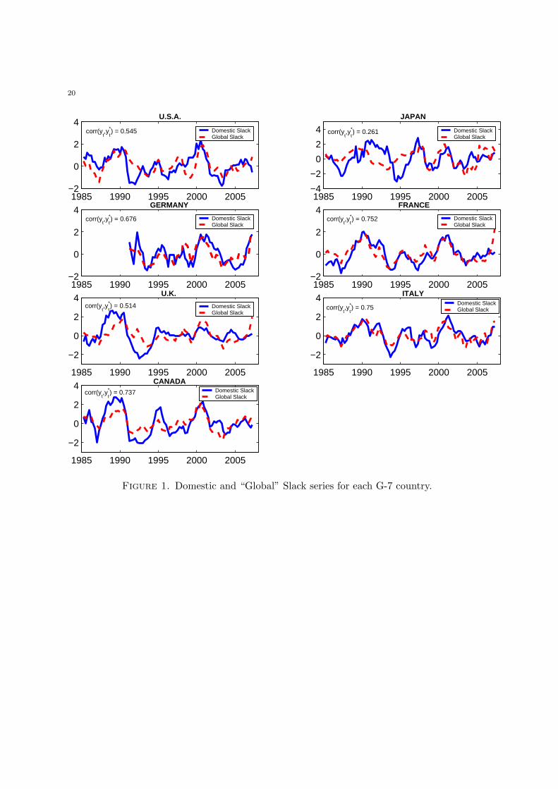
Figure 1 displays the domestic output gap along with the corresponding global output gap
series for each country in the sample. The correlation between the domestic and global output
gap series ranges from 0.261 for Japan to 0.75 for Italy and France: although the two strongly
comove, the correlations are never so high as to create problems of near-perfect collinearity in
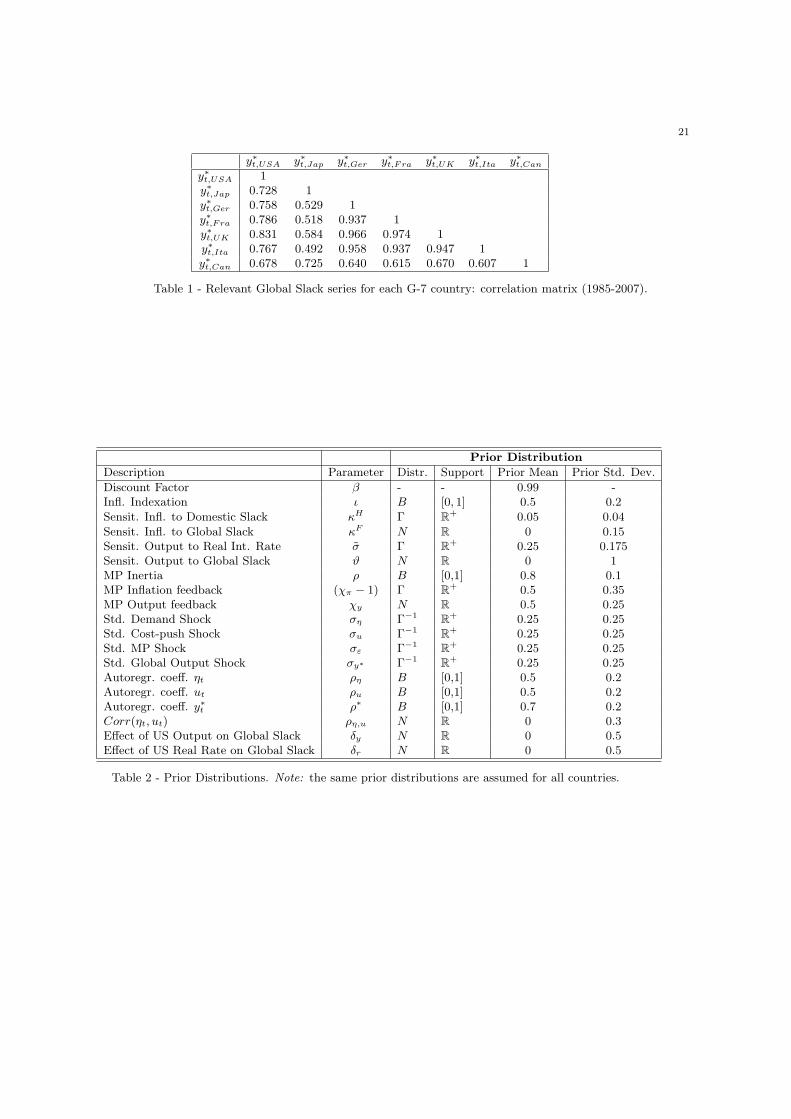
the estimation. The relevant foreign output series for the European countries in the sample
appear very similar to each other (their correlation coefficients, as shown in Table 1, are above
0.9), while the derived global slack series for the U.S., Canada, and especially Japan, are clearly
distinct (for example, the correlation coefficients between global slack for Japan and those for
European countries are around 0.5).
inferring a reliable theoretical measure of “global output gap” (e.g., Wynne and Solomon, 2007), I prefer hereto focus on a widely used statistical measure.
8In few cases, data for a trading partner are available only at the annual, but not quarterly frequency: thesecountries are dropped from the analysis (these cases, however, are marginal, as they refer to countries withweights wi
t,j close to zero, and, therefore, unlikely to have sizeable effects on the results). When data are insteadnot available starting from 1985 for some trading partners, the countries are assigned a zero weight until thefirst quarter of available data, when they start being included in the global slack calculation.
11
4. Does Global Output Affect Domestic Inflation Rates?
The model is estimated using Bayesian methods to fit the data on detrended output, do-
mestic inflation rates, nominal interest rates, and the relevant global output measure for each
G-7 country (all variables are demeaned before the estimation). The sample in the estimation
starts from 1985:q1 and ends in 2007:q1 (with the exception of Germany, for which only post-
unification data are used and the sample is 1991:q1-2007:q1): the starting date is selected both
to be consistent with the choice in Borio and Filardo (2007) and Ihrig et al. (2007) and because
the pace of globalization has significantly accelerated after the mid-1980s. The coefficients to
be estimated for each country are collected in the vector Θ
Θ ={ι, κH , κF , σ, ϑ, ρ, χπ, χy, ρη, ρu, ρ∗, ση, σu, σε, ρη,u
}. (4.1)
The priors for the coefficients in Θ are described in Table 2. I assume a Gamma prior dis-
tribution with mean 0.05 and standard deviation 0.04 for the coefficient κH and a Normal
distribution with mean 0 and standard deviation 0.15 for the main parameter of interest κF :
as there is not much existing evidence on the value of this parameter, the prior is centered at 0
and does not constrain κF to be positive; its sign is, in fact, ambiguous from the theory. The
effect of the domestic output gap on inflation, instead, is restricted to be positive. I assume
a Normal prior distribution for ϑ with mean 0 and standard deviation 1: again, this prior is
meant to be rather uninformative, both in terms of sign and magnitude, about the sensitivity
of domestic to global variables. The coefficient σ follows a Gamma with mean 0.25 and stan-
dard deviation 0.175.9 As regards the monetary policy rule coefficients, (χπ − 1) has a prior
Gamma distribution with mean 0.5 and standard deviation 0.35 (all the prior probability is
hence placed on values of χπ above 1 to ensure that the Taylor principle is satisfied, which
seems sensible for post-1985 monetary policies), and χy has a normal prior distribution with
mean 0.5 and standard deviation 0.25.10 All the autoregressive coefficients follow Beta prior
distributions, while inverse Gamma priors are used for the standard deviations of the shocks
9I have repeated the estimation with a prior for σ with a larger mean (Gamma prior with mean 1 andstandard deviation 0.7), but the empirical conclusions are unaffected.
10The paper implicitly assumes that there are no significant differences in the pre- and post-ECB monetarypolicy rule coefficients for Euro-area countries. While monetary policy is common in the Euro area, the Taylorrules in the model include only country-specific variables. This assumption is unlikely to have any influenceon the main results of interest. As a check, however, I re-estimate the models stopping the sample in 1998for Germany, France, and Italy, and report the results in the robustness section. The main conclusions in theempirical analysis are unchanged.
12
and a N(0, 0.32) prior distribution is assumed for the correlation coefficient ρη,u between the
demand and supply shocks. The discount factor is, instead, treated as fixed in the estimation:
β = 0.99.
As the model is linear and the shocks are assumed to be normally-distributed, its likelihood
can be derived using the Kalman filter at each iteration of the Metropolis-Hastings algorithm,
which is used to sample from the posterior distribution (the estimation techniques are reviewed
in detail in An and Schorfheide, 2008). For each country, I estimate the model by running five
chains of 500,000 draws each, discarding the first 125,000 as initial burn-in.
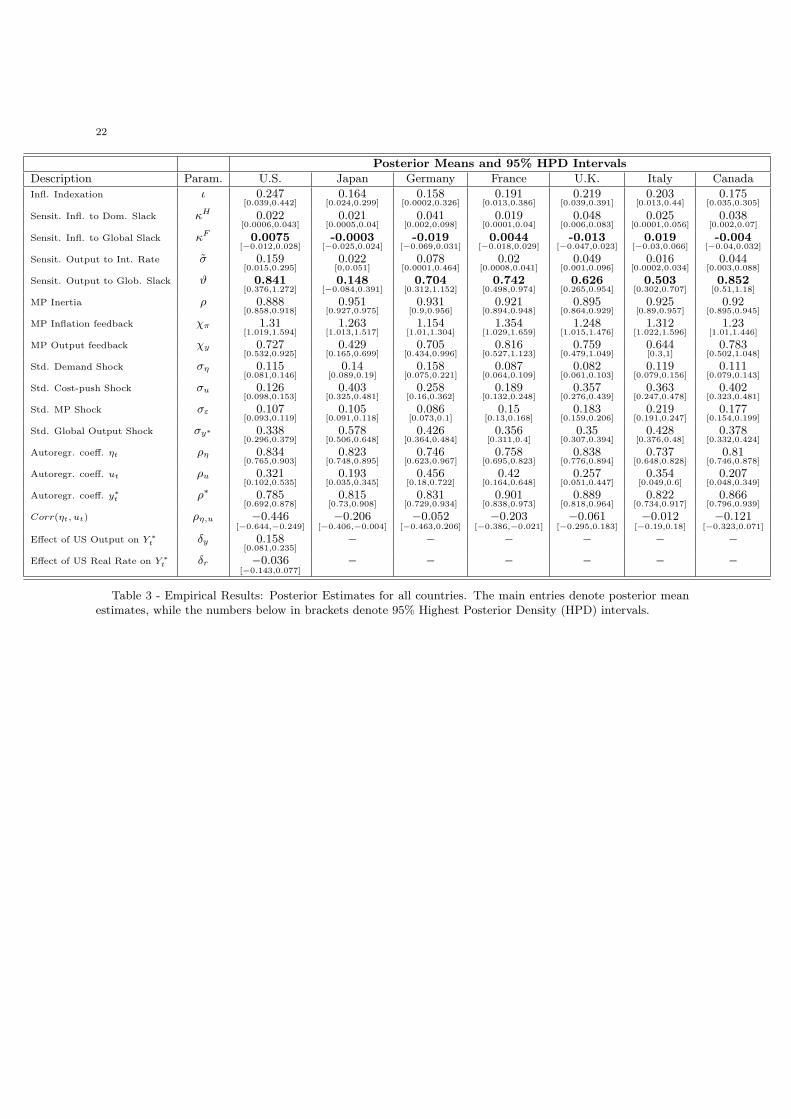
4.1. Posterior Estimates. Table 3 shows the estimation results regarding the baseline model
for each G-7 country treated in turn as the relevant domestic economy.
The posterior mean estimates for κF , which denotes the sensitivity of domestic inflation to
global slack, are positive and equal to 0.019 for Italy, 0.0075 for the United States, and 0.0044
for France. The 95% highest posterior density intervals, however, never fall entirely above 0:
the probability of κF being above zero given the data reaches 75% for Italy and the U.S. In the
other cases, global slack enters the inflation equation with a negative sign (although typically
close to zero): the posterior mean for κF equals -0.0003 for Japan, -0.004 for Canada, -0.013
for the U.K., and -0.019 for Germany. A negative sign has also been often found by Ihrig et al.
(2007) and it is not inconsistent with the theory, which leaves the sign of κF ambiguous (e.g.,
CGG, 2002, Woodford, 2007). The estimates for the sensitivity of inflation rates to domestic
slack, denoted by κH , range from 0.019 for France to 0.048 for the U.K.
The results, however, do not imply that global slack does not play any role in most G-7
economies. The estimates, in fact, reveal a large impact of global output on domestic output.
The posterior mean estimates for the coefficient ϑ are equal to 0.852 for Canada, 0.742 for
France, 0.704 for Germany, 0.626 for the U.K., and 0.503 for Italy. The U.S. business cycle
is also affected by global economic developments (ϑ = 0.841). The only country in which the
effect of global slack on domestic aggregate demand is modest is Japan: the mean estimate
for ϑ is 0.148; the small effect is probably due to the particular developments in the Japanese
economy in the sample (which includes Japan’s “lost decade” years), which were largely driven
by internal, rather than global, factors.
Turning to the other coefficients, the degrees of inflation indexation in the post-1985 sample
are limited in most countries (the values of ι range from 0.158 in Germany to 0.247 in the U.S.).

13
As the U.S. are usually regarded as an engine of global economic growth, in the estimation
with the U.S. as the Home country, global output is allowed to depend on past U.S. output
and real interest rates: the posterior mean for the coefficients denoting the sensitivity of global
output to U.S. output (δy) is equal to 0.158 and to U.S. real interest rates (δr) is equal to -0.036
(Milani, 2009, finds that the dependence on U.S. variables is larger in the pre-1979 period than
in the post-1985 period).
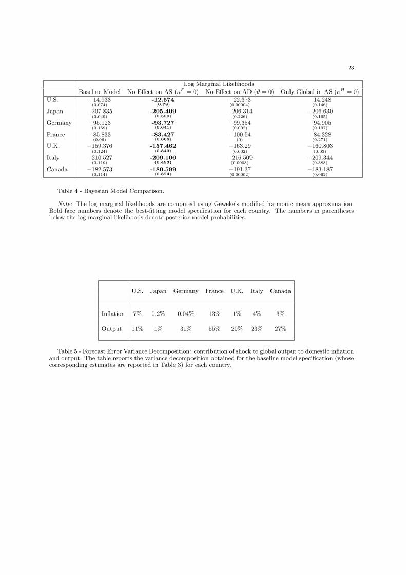
4.2. Model Comparison. To fully assess the role of global slack, besides looking at the
posterior estimates, one needs to verify whether its inclusion in the model improves the model’s
ability to fit the data and which channels are important.
The contribution of global slack is, therefore, evaluated by re-estimating the model for each
country and shutting down, in turn, either the foreign output effect through aggregate supply
(by setting κF = 0) or the foreign output effect through aggregate demand (by setting ϑ = 0).
The models’ marginal likelihoods in these two alternative cases are then compared with the
marginal likelihood from the baseline model (in which both domestic and global slack are
included and whose estimates are reported in Table 3). Finally, I also consider a specification
in which the effect of domestic output on inflation is shut down (setting κH = 0): only global
slack enters the Phillips curve.
The log marginal likelihoods are shown in Table 4, along with the implied posterior model
probabilities. The inclusion of global output leads to improvements in the models’ ability
to fit the data. The aggregate demand effect is important for all countries: the marginal
likelihoods, in fact, substantially decrease when that channel is shut down (ϑ = 0). On the
other hand, there isn’t much evidence of a direct effect of global output on domestic inflation
in the sample of countries. The best specification for all countries is one in which global slack
enters the domestic IS equation, but not the supply equation. These model specifications are
characterized by posterior model probabilities that extend from 0.6 to above 0.8. There is some
uncertainty about the best model specification, however, for Italy and France: in these cases,
the models with global-centric Phillips curves attain posterior probabilities between 0.27 and
0.39. Overall, however, for the majority of countries, the estimation does not provide much
evidence in support of altering traditional New Keynesian Phillips curves to include measures
of global slack.
14
Through its effect on domestic output, however, global output may still play an important
role in the determination of domestic inflation rates. To verify the contribution of global slack
to fluctuations in inflation, I compute the forecast error variance decomposition implied by
the model. Table 5 shows that innovations to global output can account for more than 20%
of output fluctuations in the U.K., Italy, and Canada, for 31% in Germany, and for 55% in
France. Business cycles in these countries, therefore, are to a large extent affected by external
economic conditions. Mostly through that channel, global output shocks can also account
for 13% of inflation fluctuations in France and for a smaller fraction in Canada and Italy
(3-4%). Although global output has an important effect on domestic output in Germany, the
spillovers to inflation are trivial. The contribution of global output to domestic macroeconomic
variables is, instead, smaller in the U.S. and in Japan: global shocks account for 11% of the
output variance in the U.S. and for 7% of the inflation variance, while the effects on Japanese
variables are meager.
An implication of the empirical results is that globalization is unlikely to have induced
important changes in the way monetary policy should operate. The estimates, in fact, suggest
that monitoring global slack may be worthwhile as it influences domestic output in several
countries. But the effects on inflation are still rather limited and, therefore, the effectiveness
of national policies is in no way compromised (Woodford, 2007, shows that this is true even
for scenarios in which the effects from foreign output are larger). Moreover, as the benefits of
international monetary policy cooperation typically hinge on the values of the spillover effect
κF (e.g., CGG, 2002), the estimates suggest that these benefits still remain small.
4.3. Robustness.
4.3.1. Trend in Inflation. Previous papers have found that assumptions about the existence of
a trend in inflation may affect the estimates of coefficients in the Phillips curve (e.g., Cogley
and Sbordone, 2008). In the baseline estimation, no trends have been removed from inflation,
since trends are not immediately apparent in the post-1985 sample. To verify the sensitivity
of the empirical results, however, the models are re-estimated for each country using now a
detrended measure (using the HP filter) of inflation as an observable endogenous variable: the
trend is meant to account for changes in the Fed’s long-run inflation target. The dependent
variable is now in the same spirit as the inflation gap studied in Cogley et al. (2009). The new
15
implied estimates for κH and κF are shown in Table 6 and do not alter the main conclusions:
the global slack term often enters the Phillips curve with a negative coefficient and typically
one very close to zero (all the results described in the previous section also remain unchanged).
The estimates for the other coefficients are similar: the only noticeable changes refer to the
indexation coefficient and the autocorrelation of the cost-push shock, which fall closer to zero
(an indexation coefficient near 0 is consistent with the results in Cogley and Sbordone, 2008,
who find that, after accounting for trend inflation, no backward-looking terms are necessary
in the inflation equation).
4.3.2. Euro-Area Monetary Policy. To check whether not accounting for changes in pre- and
post-ECB monetary policy in the Euro area has any effects on the results, I re-estimate the
models for France, Germany, and Italy with a sample that now ends in 1998:q4. The estimates
are comparable to those in Table 3 (κF is equal to 0.017 for France, -0.01 for Germany, and
0.013 for Italy) and the model rankings remain unaltered.
4.3.3. Priors’ Choice. In the cases of Italy, France, and the U.S., some uncertainty remains
about the results, as global slack is estimated to be a positive determinant of their inflation
rates, yet the model rankings favor specifications that exclude global slack from the Phillips
curve. The model comparison results, however, may depend on the choice of the prior distri-
butions, particularly about the coefficients κH and κF . Assuming a more informative prior
distribution about κF , in particular, would have led to more favorable evidence for the model
with global output gap also entering the inflation equation. For the U.S., the specification
preferred by the data, however, still remains the one that imposes κF = 0 even if a tight prior
with standard deviation around 0.025 is assumed for κF . For France and Italy, the marginal
likelihoods of the different specifications become much closer with a prior standard deviation
for κF equal to 0.05, and the model rankings may switch for lower standard deviations (in light
of the mixed evidence on the sensitivity of inflation to global slack coming from previous lit-
erature, however, holding such an informative prior seems unlikely before observing the data).
As a further check, I also increase the mean and standard deviation for the prior on κH (now
a Gamma with mean 0.1 and std. 0.08) and repeat the estimation: the model rankings do not
change for the U.S., while they switch for France (the models’ marginal likelihoods remain very
close to each other for Italy). The estimated coefficients in the baseline models, instead, do

16
not change. Therefore, the conclusion from the variance decomposition that shocks to global
output can account for a modest portion of inflation fluctuations in these countries is robust.
4.3.4. Correlation Among Shocks. The baseline estimation has assumed that shocks to do-
mestic and global output gaps were uncorrelated. I now allow these shocks to be correlated
and re-estimate the models for the U.S., France, and Italy. The largest estimated correlation
coefficient is equal to 0.097, obtained for the U.S. specification; the remaining coefficients and
the model comparison conclusions do not vary.
5. Conclusions
Recent studies have suggested an important role for global output as a variable driving
domestic inflation rates.
This paper has investigated its empirical importance by estimating a structural model, which
captures the potential effects of global output on the domestic aggregate supply and demand
relations in the economy, for each G-7 country.
The empirical results indicate that global output fluctuations have a non-negligible impact
on domestic demand in most countries. Through this channel, the global output gap can
also affect domestic inflation rates. The direct impact of global slack on marginal costs and
inflation, however, appears less central: the data, in fact, favor model specifications in which
global slack enters the IS curve, but generally they do not provide clear evidence in favor of
altering closed-economy Phillips curves to include global slack as an additional driving variable.
There are other channels through which globalization may affect the behavior of inflation
and which have been omitted in the current paper. For example, the frequency of price changes
may be made endogenous and allowed to depend on the degree of competition, which may be
itself a function of the economy’s openness to trade. The paper has also abstracted from the
channels recently emphasized by Sbordone (2007) and Guerrieri et al. (2007). Extending the
model in these directions may give a broader view of the empirical consequences of globalization
on inflation dynamics.
Moreover, the empirical evidence in this paper has been obtained in the context of a small-
scale structural model of the type used in Ireland (2004) and Lubik and Schorfheide (2004),
but extended to allow for a potential role of global output measures. It is left to future research
17
to check the role of global slack in medium and large-scale settings as the Smets and Wouters
(2002)’s model, the Federal Reserve’s Sigma model, or the ECB’s New Area-Wide Model.
References
[1] An, S., and F. Schorfheide, (2007). “Bayesian Analysis of DSGE Models”, Econometric Reviews, Vol. 26,Issue 2-4, pages 113-172.
[2] Ball, L., (2006). “Has Globalization Changed Inflation?”, NBER Working Paper 12687.[3] Benigno, G., and P. Benigno, (2006). “Designing Targeting Rules For International Monetary Policy Co-
operation,” Journal of Monetary Economics, Vol. 53, Iss. 3, 473-506.[4] Bernanke, B., (2007). “Globalization and Monetary Policy”, Speech to Stanford Institute for Economic
Policy Research, March 2.[5] Borio, C., and A. Filardo, (2007). “Globalisation and Inflation: New Cross-Country Evidence on the Global
Determinants of Domestic Inflation,” Working Paper No 227, Bank for International Settlements.[6] Calza, A., (2008). “Globalisation, Domestic Inflation and Global Output Gaps: Evidence from the Euro
Area”, European Central Bank Working Paper No. 890.[7] Castelnuovo, E., (2007). “Tracking U.S. Inflation Expectations with Domestic and Global Determinants,”
mimeo, University of Padua.[8] Christiano, L. J., Eichenbaum, M., and C. L. Evans, (2005). “Nominal Rigidities and the Dynamic Effects
of a Shock to Monetary Policy,” Journal of Political Economy, vol. 113(1), pages 1-45.[9] Ciccarelli, M., and B. Mojon, (2009). “Global Inflation,” Review of Economics and Statistics, forthcoming.
[10] Clarida, R., J. Galı, and M. Gertler, (2002). “A Simple Framework for International Monetary PolicyAnalysis”, Journal of Monetary Economics, 49, 879-904.
[11] Coenen, G., Lombardo, G., Smets, F., and R. Straub, (2007). “International Transmission And MonetaryPolicy Cooperation”, in J. Gali and M. J. Gertler ed., International Dimensions of Monetary Policy,University of Chicago Press.
[12] Cogley, T., Primiceri, G., and T. J. Sargent, (2009). “Inflation-Gap Persistence in the U.S.”, AmericanEconomic Journal: Macroeconomics, forthcoming.
[13] Cogley, T., and A. M. Sbordone, (2008). “Trend Inflation, Indexation, and Inflation Persistence in the NewKeynesian Phillips Curve”, American Economic Review, 98(5): 21012126.
[14] D’Agostino, A., and P. Surico, (2009). “Does Global Liquidity Help to Forecast US Inflation?”, Journal ofMoney, Credit and Banking, forthcoming.
[15] Fisher, R., (2005). “Globalization and Monetary Policy”, Warren and Anita Manshel Lecture in AmericanForeign Policy, Harvard University, Cambridge, MA.
[16] Forbes, K. J., and M. D. Chinn, (2004). “A Decomposition of Global Linkages in Financial Markets OverTime,” The Review of Economics and Statistics, vol. 86(3), pages 705-722.
[17] Gamber, E. N., and J. H. Hung, (2001), “Has the Rise in Globalization Reduced U.S. Inflation in the1990s?”, Economic Inquiry, Volume 39, Issue 1, Page 58-73.
[18] Guerrieri, L., Gust, C., and D. Lopez-Salido, (2008). “International Competition and Inflation: A NewKeynesian Perspective”, Board of Governors of the Federal Reserve System, Working Paper No. 918.
[19] Ihrig, J., Kamin, S. B., Lindner, D., and J. Marquez, (2007). “Some Simple Tests of the Globalization andInflation Hypothesis,” Board of Governors of the Federal Reserve System, IF Discussion Paper No. 891.
[20] Ireland, P.N., (2004). “Technology Shocks in the New Keynesian Model,” The Review of Economics andStatistics, vol. 86(4), 923-936.
[21] Lubik, T.A., and F. Schorfheide, (2004). “Testing for Indeterminacy: An Application to U.S. MonetaryPolicy,” American Economic Review, vol. 94(1), 190-217.
[22] Kohn, D. L., (2006). “The Effects of Globalization on Inflation and Their Implications for Monetary Policy”,Speech at the Federal Reserve Bank of Boston’s 51st Economic Conference, Chatham, Massachusetts.
[23] Milani, F., (2009). “Has Global Slack Become More Important than Domestic Slack in Determining U.S.Inflation?”, Economics Letters, Volume 102, Issue 3, pages 147-151.
[24] Mumtaz, H., and P. Surico, (2008). “Evolving International Inflation Dynamics: World and Country SpecificFactors”, CEPR discussion paper No 6767.
[25] Razin, A., and C.W. Yuen, (2002) “The ‘New Keynesian’ Phillips Curve: Closed Economy versus OpenEconomy,” Economics Letters 75, 1-9.
[26] Razin, A., and P. Loungani, (2005). “Globalization and Inflation-Output Tradeoffs,” NBER Working Paper11641.
18
[27] Razin A. and A. Binyamini, (2007). “Flattened Inflation-Output Tradeoff and Enhanced Anti-InflationPolicy: Outcome of Globalization?” NBER Working Paper 13280.
[28] Rogoff, K.S., (2003) “Globalization and Global Disinflation” in Monetary Policy and Uncertainty: Adaptingto a Changing Economy, Federal Reserve Bank of Kansas City.
[29] Rogoff, K.S., (2006) “Impact of Globalization on Monetary Policy,” in The New Economic Geography:Effects and Policy Implications, Federal Reserve Bank of Kansas City.
[30] Romer, D., (1993). “Openness and Inflation: Theory and Evidence”, The Quarterly Journal of Economics,Vol. 108, No. 4, pp. 869-903.
[31] Sbordone, A., (2007). “Globalization and Inflation Dynamics: The Impact of Increased Competition,” inJ. Gali and M. J. Gertler ed., International Dimensions of Monetary Policy, University of Chicago Press.
[32] Smets, F., and R. Wouters, (2002). “Openness, Imperfect Exchange Rate Pass-Through and MonetaryPolicy”, Journal of Monetary Economics, Vol. 49(5), 947-981.
[33] Tootell, G., (1998). “Globalization and U.S. Inflation”, Federal Reserve Bank of Boston, New EnglandEconomic Review, pp. 21-33.
[34] Woodford, M. (2007) “Globalization and Monetary Control,” in J. Gali and M. J. Gertler ed., InternationalDimensions of Monetary Policy, University of Chicago Press.
[35] Wynne, M.A., and E.K. Kersting (2007), “Openness and Inflation,” Federal Reserve of Dallas Staff PaperNo. 2.
[36] Wynne, M.A., and G.R. Solomon, (2007). “Obstacles to Measuring Global Output Gaps,” Federal ReserveBank of Dallas Economic Letter, vol. 2.
[37] Zaniboni, N., (2008). “Globalization and the Phillips Curve”, mimeo, Princeton University.
19
Appendix A. Construction of Global Slack Series.
Data on U.S. real GDP, GDP implicit price deflator, and the Federal Funds rate were obtained fromFRED R©, the Federal Reserve of St. Louis Economic Database. All data on real GDP, GDP implicitprice deflators, and nominal interest rates for the remaining G-7 countries, on real GDP for the tradingpartners included in the calculation of the “global slack” series, and on bilateral imports and exports,were downloaded from IHS Global Insight.
The measure of global slack, denoted by y∗t in the model, has been calculated for each G-7 countryusing data on real GDP (NCUs, seasonally adjusted, detrended using the HP filter, with smoothingparameter λ = 1, 600) for the following lists of trading partners:
• U.S.A.: Argentina, Australia, Austria, Belgium, Brazil, Canada, Chile, China, Colombia,Costa Rica, Denmark, Ecuador, Finland, France, Germany, Hong Kong, India, Indonesia,Ireland, Israel, Italy, Japan, Korea, Malaysia, Mexico, Netherlands, Norway, New Zealand,Philippines, Russia, South Africa, Singapore, Spain, Sweden, Switzerland, Thailand, Turkey,U.K., Venezuela.
• JAPAN: Australia, Brazil, Canada, China, France, Germany, Hong Kong, India, Indonesia,Italy, Korea, Malaysia, Mexico, Netherlands, New Zealand, Philippines, Russia, Singapore,South Africa, Spain, Switzerland, Thailand, U.K., U.S.A.
• GERMANY: Austria, Belgium, Brazil, Canada, China, Czech Republic, Denmark, Finland,France, Greece, Hong Kong, Hungary, Ireland, Italy, Japan, Korea, Netherlands, Norway,Poland, Portugal, Russia, Singapore, South Africa, Spain, Sweden, Switzerland, Turkey, U.K.,U.S.A..
• FRANCE: Austria, Belgium, Brazil, Canada, China, Denmark, Finland, Germany, Greece,Ireland, Italy, Japan, Korea, Netherlands, Norway, Poland, Portugal, Russia, Singapore, Spain,Sweden, Switzerland, Tunisia, Turkey, U.K., U.S.A.
• U.K.: Australia, Austria, Belgium, Canada, China, Denmark, Finland, France, Germany, HongKong, India, Ireland, Italy, Japan, Korea, Malaysia, Netherlands, Norway, Portugal, Russia,Singapore, South Africa, Spain, Sweden, Switzerland, Turkey, U.S.A.
• ITALY: Austria, Belgium, Brazil, Canada, China, Denmark, France, Germany, Greece, Hun-gary, Ireland, Japan, Korea, Netherlands, Poland, Portugal, Romania, Russia, South Africa,Spain, Sweden, Switzerland, Turkey, U.K., U.S.A.
• CANADA: Australia, Belgium, Brazil, China, France, Germany, Hong Kong, India, Indone-sia, Ireland, Italy, Japan, Korea, Malaysia, Mexico, Netherlands, Norway, Philippines, Singa-pore, Spain, Sweden, Switzerland, Thailand, U.K., U.S.A., Venezuela.
20
1985 1990 1995 2000 2005−2
0
2
4U.S.A.
corr(yt,y
t*) = 0.545 Domestic Slack
Global Slack
1985 1990 1995 2000 2005−4
−2
0
2
4
JAPAN
corr(yt,y
t*) = 0.261 Domestic Slack
Global Slack
1985 1990 1995 2000 2005−2
0
2
4GERMANY
corr(yt,y
t*) = 0.676 Domestic Slack
Global Slack
1985 1990 1995 2000 2005−2
0
2
4FRANCE
corr(yt,y
t*) = 0.752 Domestic Slack
Global Slack
1985 1990 1995 2000 2005
−2
0
2
4 U.K.
corr(yt,y
t*) = 0.514 Domestic Slack
Global Slack
1985 1990 1995 2000 2005
−2
0
2
4 ITALY
corr(yt,y
t*) = 0.75
Domestic SlackGlobal Slack
1985 1990 1995 2000 2005
−2
0
2
4 CANADAcorr(y
t,y
t*) = 0.737 Domestic Slack
Global Slack
Figure 1. Domestic and “Global” Slack series for each G-7 country.
21
y∗t,USA y∗t,Jap y∗t,Ger y∗t,Fra y∗t,UK y∗t,Ita y∗t,Can
y∗t,USA 1y∗t,Jap 0.728 1y∗t,Ger 0.758 0.529 1y∗t,Fra 0.786 0.518 0.937 1y∗t,UK 0.831 0.584 0.966 0.974 1y∗t,Ita 0.767 0.492 0.958 0.937 0.947 1y∗t,Can 0.678 0.725 0.640 0.615 0.670 0.607 1
Table 1 - Relevant Global Slack series for each G-7 country: correlation matrix (1985-2007).
Prior Distribution
Description Parameter Distr. Support Prior Mean Prior Std. Dev.
Discount Factor β - - 0.99 -Infl. Indexation ι B [0, 1] 0.5 0.2Sensit. Infl. to Domestic Slack κH Γ R+ 0.05 0.04Sensit. Infl. to Global Slack κF N R 0 0.15Sensit. Output to Real Int. Rate σ Γ R+ 0.25 0.175Sensit. Output to Global Slack ϑ N R 0 1MP Inertia ρ B [0,1] 0.8 0.1MP Inflation feedback (χπ − 1) Γ R+ 0.5 0.35MP Output feedback χy N R 0.5 0.25Std. Demand Shock ση Γ−1 R+ 0.25 0.25Std. Cost-push Shock σu Γ−1 R+ 0.25 0.25Std. MP Shock σε Γ−1 R+ 0.25 0.25Std. Global Output Shock σy∗ Γ−1 R+ 0.25 0.25Autoregr. coeff. ηt ρη B [0,1] 0.5 0.2Autoregr. coeff. ut ρu B [0,1] 0.5 0.2Autoregr. coeff. y∗t ρ∗ B [0,1] 0.7 0.2Corr(ηt, ut) ρη,u N R 0 0.3Effect of US Output on Global Slack δy N R 0 0.5Effect of US Real Rate on Global Slack δr N R 0 0.5
Table 2 - Prior Distributions. Note: the same prior distributions are assumed for all countries.
22
Posterior Means and 95% HPD Intervals
Description Param. U.S. Japan Germany France U.K. Italy Canada
Infl. Indexation ι 0.247[0.039,0.442]
0.164[0.024,0.299]
0.158[0.0002,0.326]
0.191[0.013,0.386]
0.219[0.039,0.391]
0.203[0.013,0.44]
0.175[0.035,0.305]
Sensit. Infl. to Dom. Slack κH 0.022[0.0006,0.043]
0.021[0.0005,0.04]
0.041[0.002,0.098]
0.019[0.0001,0.04]
0.048[0.006,0.083]
0.025[0.0001,0.056]
0.038[0.002,0.07]
Sensit. Infl. to Global Slack κF 0.0075[−0.012,0.028]
-0.0003[−0.025,0.024]
-0.019[−0.069,0.031]
0.0044[−0.018,0.029]
-0.013[−0.047,0.023]
0.019[−0.03,0.066]
-0.004[−0.04,0.032]
Sensit. Output to Int. Rate σ 0.159[0.015,0.295]
0.022[0,0.051]
0.078[0.0001,0.464]
0.02[0.0008,0.041]
0.049[0.001,0.096]
0.016[0.0002,0.034]
0.044[0.003,0.088]
Sensit. Output to Glob. Slack ϑ 0.841[0.376,1.272]
0.148[−0.084,0.391]
0.704[0.312,1.152]
0.742[0.498,0.974]
0.626[0.265,0.954]
0.503[0.302,0.707]
0.852[0.51,1.18]
MP Inertia ρ 0.888[0.858,0.918]
0.951[0.927,0.975]
0.931[0.9,0.956]
0.921[0.894,0.948]
0.895[0.864,0.929]
0.925[0.89,0.957]
0.92[0.895,0.945]
MP Inflation feedback χπ 1.31[1.019,1.594]
1.263[1.013,1.517]
1.154[1.01,1.304]
1.354[1.029,1.659]
1.248[1.015,1.476]
1.312[1.022,1.596]
1.23[1.01,1.446]
MP Output feedback χy 0.727[0.532,0.925]
0.429[0.165,0.699]
0.705[0.434,0.996]
0.816[0.527,1.123]
0.759[0.479,1.049]
0.644[0.3,1]
0.783[0.502,1.048]
Std. Demand Shock ση 0.115[0.081,0.146]
0.14[0.089,0.19]
0.158[0.075,0.221]
0.087[0.064,0.109]
0.082[0.061,0.103]
0.119[0.079,0.156]
0.111[0.079,0.143]
Std. Cost-push Shock σu 0.126[0.098,0.153]
0.403[0.325,0.481]
0.258[0.16,0.362]
0.189[0.132,0.248]
0.357[0.276,0.439]
0.363[0.247,0.478]
0.402[0.323,0.481]
Std. MP Shock σε 0.107[0.093,0.119]
0.105[0.091,0.118]
0.086[0.073,0.1]
0.15[0.13,0.168]
0.183[0.159,0.206]
0.219[0.191,0.247]
0.177[0.154,0.199]
Std. Global Output Shock σy∗ 0.338[0.296,0.379]
0.578[0.506,0.648]
0.426[0.364,0.484]
0.356[0.311,0.4]
0.35[0.307,0.394]
0.428[0.376,0.48]
0.378[0.332,0.424]
Autoregr. coeff. ηt ρη 0.834[0.765,0.903]
0.823[0.748,0.895]
0.746[0.623,0.967]
0.758[0.695,0.823]
0.838[0.776,0.894]
0.737[0.648,0.828]
0.81[0.746,0.878]
Autoregr. coeff. ut ρu 0.321[0.102,0.535]
0.193[0.035,0.345]
0.456[0.18,0.722]
0.42[0.164,0.648]
0.257[0.051,0.447]
0.354[0.049,0.6]
0.207[0.048,0.349]
Autoregr. coeff. y∗t ρ∗ 0.785[0.692,0.878]
0.815[0.73,0.908]
0.831[0.729,0.934]
0.901[0.838,0.973]
0.889[0.818,0.964]
0.822[0.734,0.917]
0.866[0.796,0.939]
Corr(ηt, ut) ρη,u −0.446[−0.644,−0.249]
−0.206[−0.406,−0.004]
−0.052[−0.463,0.206]
−0.203[−0.386,−0.021]
−0.061[−0.295,0.183]
−0.012[−0.19,0.18]
−0.121[−0.323,0.071]
Effect of US Output on Y ∗t δy 0.158[0.081,0.235]
− − − − − −Effect of US Real Rate on Y ∗t δr −0.036
[−0.143,0.077]− − − − − −
Table 3 - Empirical Results: Posterior Estimates for all countries. The main entries denote posterior meanestimates, while the numbers below in brackets denote 95% Highest Posterior Density (HPD) intervals.
23
Log Marginal Likelihoods
Baseline Model No Effect on AS (κF = 0) No Effect on AD (ϑ = 0) Only Global in AS (κH = 0)
U.S. −14.933(0.074)
-12.574(0.78)
−22.373(0.00004)
−14.248(0.146)
Japan −207.835(0.049)
-205.409(0.559)
−206.314(0.226)
−206.630(0.165)
Germany −95.123(0.159)
-93.727(0.641)
−99.354(0.002)
−94.905(0.197)
France −85.833(0.06)
-83.427(0.668)
−100.54(0)
−84.328(0.271)
U.K. −159.376(0.124)
-157.462(0.843)
−163.29(0.002)
−160.803(0.03)
Italy −210.527(0.119)
-209.106(0.493)
−216.509(0.0003)
−209.344(0.388)
Canada −182.573(0.114)
-180.599(0.824)
−191.37(0.00002)
−183.187(0.062)
Table 4 - Bayesian Model Comparison.
Note: The log marginal likelihoods are computed using Geweke’s modified harmonic mean approximation.Bold face numbers denote the best-fitting model specification for each country. The numbers in parenthesesbelow the log marginal likelihoods denote posterior model probabilities.
U.S. Japan Germany France U.K. Italy Canada
Inflation 7% 0.2% 0.04% 13% 1% 4% 3%
Output 11% 1% 31% 55% 20% 23% 27%
Table 5 - Forecast Error Variance Decomposition: contribution of shock to global output to domestic inflationand output. The table reports the variance decomposition obtained for the baseline model specification (whosecorresponding estimates are reported in Table 3) for each country.

24
Description Param. U.S. Japan Germany France U.K. Italy Canada
Sensit. Infl. to Dom. Slack κH 0.013[0.0003,0.02]
0.025[0.002,0.04]
0.032[0.0004,0.07]
0.022[0.0003,0.04]
0.04[0.01,0.07]
0.027[0.0004,0.05]
0.036[0.004,0.07]
Sensit. Infl. to Global Slack κF 0.0085[−0.005,0.02]
−0.002[−0.02,0.02]
−0.004[−0.04,0.03]
−0.003[−0.02,0.02]
−0.015[−0.04,0.01]
0.008[−0.02,0.04]
−0.01[−0.04,0.02]
Table 6 - Robustness: Posterior Estimates for all countries (estimation with detrended inflation series). Themain entries denote posterior mean estimates, while the numbers below in brackets denote 95% Highest PosteriorDensity (HPD) intervals.