1

Global Temperature Update Through 2013

21 January 2014

James Hansen, Makiko Sato and Reto Ruedy

Summary. Global surface temperature in 2013 was +0.6°C (~1.1°F) warmer than the 1951-1980

base period average, thus the seventh warmest year in the GISS analysis. The rate of global

warming is slower in the past decade than in the prior three decades. Slower growth of net climate

forcings and cooling in the tropical Pacific Ocean both contribute to the slower warming rate, with

the latter probably the more important effect. The tropical Pacific cooling is probably unforced

variability, at least in large part. The trend toward an increased frequency of extreme hot summer

anomalies over land areas has continued despite the Pacific Ocean cooling. The “bell curves” for

observed temperature anomalies show that, because of larger unforced variability in winter, it is

more difficult in winter than in summer to recognize the effect of global warming on the occurrence

of extreme warm or cold seasons. It appears that there is substantial likelihood of an El Niño

beginning in 2014, and as a result a probable record global temperature in 2014 or 2015.

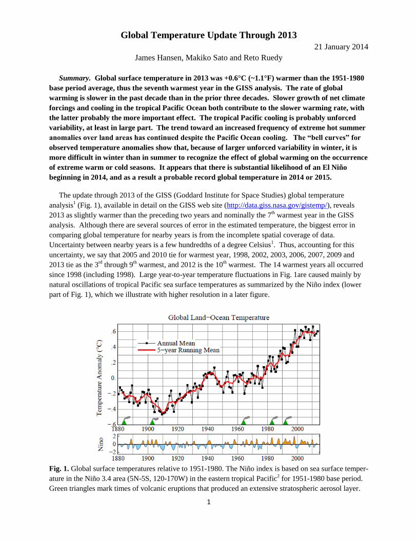
The update through 2013 of the GISS (Goddard Institute for Space Studies) global temperature

analysis1 (Fig. 1), available in detail on the GISS web site (http://data.giss.nasa.gov/gistemp/), reveals

2013 as slightly warmer than the preceding two years and nominally the 7th warmest year in the GISS

analysis. Although there are several sources of error in the estimated temperature, the biggest error in

comparing global temperature for nearby years is from the incomplete spatial coverage of data.

Uncertainty between nearby years is a few hundredths of a degree Celsius1. Thus, accounting for this

uncertainty, we say that 2005 and 2010 tie for warmest year, 1998, 2002, 2003, 2006, 2007, 2009 and

2013 tie as the 3rd

through 9th warmest, and 2012 is the 10

th warmest. The 14 warmest years all occurred

since 1998 (including 1998). Large year-to-year temperature fluctuations in Fig. 1are caused mainly by

natural oscillations of tropical Pacific sea surface temperatures as summarized by the Niño index (lower

part of Fig. 1), which we illustrate with higher resolution in a later figure.

Fig. 1. Global surface temperatures relative to 1951-1980. The Niño index is based on sea surface temper-

ature in the Niño 3.4 area (5N-5S, 120-170W) in the eastern tropical Pacific2 for 1951-1980 base period.

Green triangles mark times of volcanic eruptions that produced an extensive stratospheric aerosol layer.

2

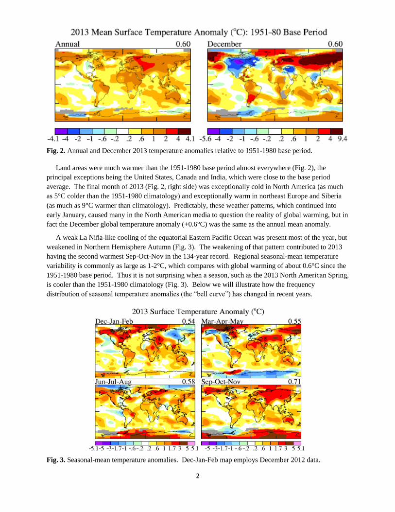
Fig. 2. Annual and December 2013 temperature anomalies relative to 1951-1980 base period.

Land areas were much warmer than the 1951-1980 base period almost everywhere (Fig. 2), the

principal exceptions being the United States, Canada and India, which were close to the base period

average. The final month of 2013 (Fig. 2, right side) was exceptionally cold in North America (as much

as 5°C colder than the 1951-1980 climatology) and exceptionally warm in northeast Europe and Siberia

(as much as 9°C warmer than climatology). Predictably, these weather patterns, which continued into

early January, caused many in the North American media to question the reality of global warming, but in

fact the December global temperature anomaly (+0.6°C) was the same as the annual mean anomaly.

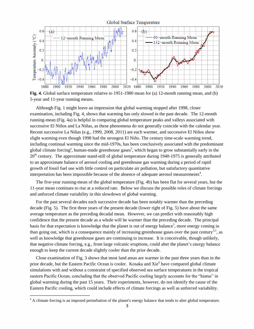
A weak La Niña-like cooling of the equatorial Eastern Pacific Ocean was present most of the year, but

weakened in Northern Hemisphere Autumn (Fig. 3). The weakening of that pattern contributed to 2013

having the second warmest Sep-Oct-Nov in the 134-year record. Regional seasonal-mean temperature

variability is commonly as large as 1-2°C, which compares with global warming of about 0.6°C since the

1951-1980 base period. Thus it is not surprising when a season, such as the 2013 North American Spring,

is cooler than the 1951-1980 climatology (Fig. 3). Below we will illustrate how the frequency

distribution of seasonal temperature anomalies (the “bell curve”) has changed in recent years.

Fig. 3. Seasonal-mean temperature anomalies. Dec-Jan-Feb map employs December 2012 data.

3

Fig. 4. Global surface temperature relative to 1951-1980 mean for (a) 12-month running mean, and (b)

5-year and 11-year running means.

Although Fig. 1 might leave an impression that global warming stopped after 1998, closer

examination, including Fig. 4, shows that warming has only slowed in the past decade. The 12-month

running-mean (Fig. 4a) is helpful in comparing global temperature peaks and valleys associated with

successive El Niños and La Niñas, as these phenomena do not generally coincide with the calendar year.

Recent successive La Niñas (e.g., 1999, 2008, 2011) are each warmer, and successive El Niños show

slight warming even though 1998 had the strongest El Niño. The century time-scale warming trend,

including continual warming since the mid-1970s, has been conclusively associated with the predominant

global climate forcinga, human-made greenhouse gases

3, which began to grow substantially early in the

20th century. The approximate stand-still of global temperature during 1940-1975 is generally attributed

to an approximate balance of aerosol cooling and greenhouse gas warming during a period of rapid

growth of fossil fuel use with little control on particulate air pollution, but satisfactory quantitative

interpretation has been impossible because of the absence of adequate aerosol measurements4.

The five-year running-mean of the global temperature (Fig. 4b) has been flat for several years, but the

11-year mean continues to rise at a reduced rate. Below we discuss the possible roles of climate forcings

and unforced climate variability in this slowdown of global warming.

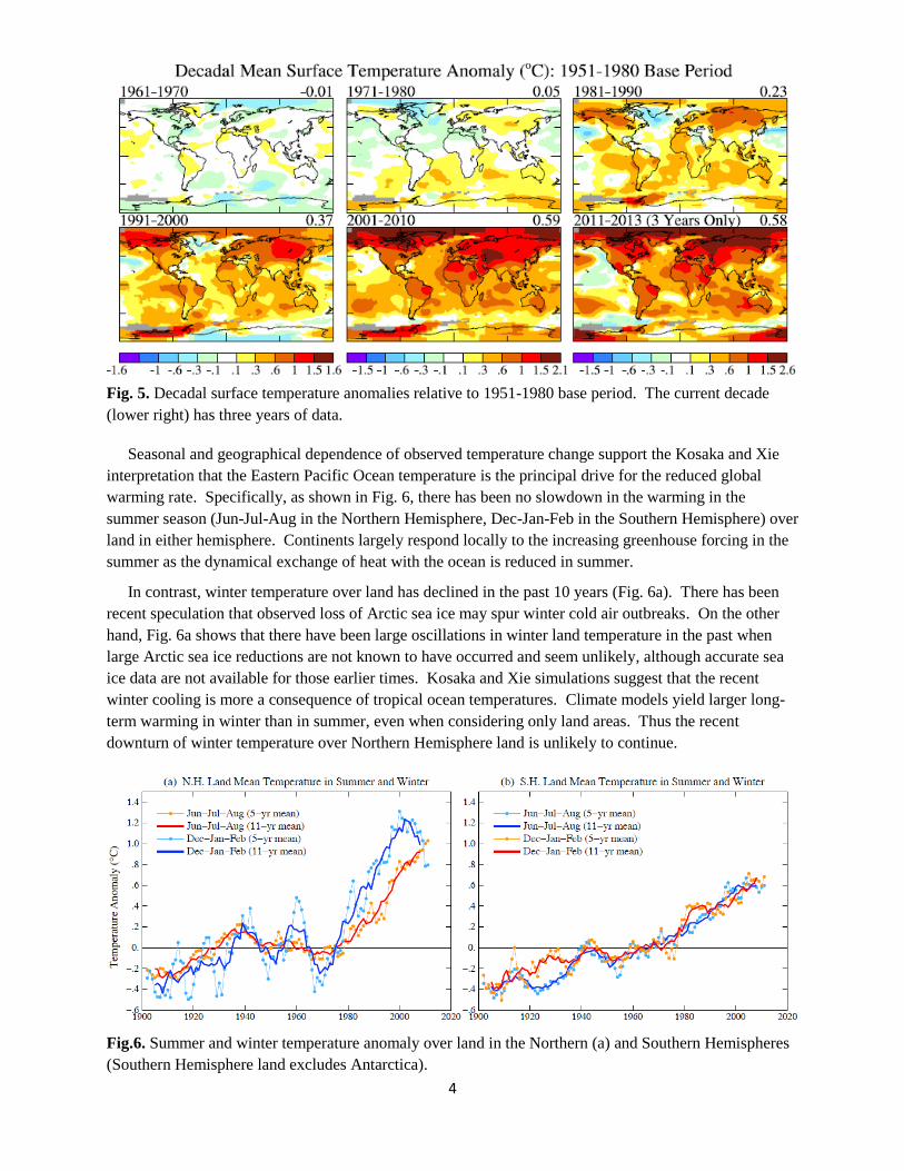
For the past several decades each successive decade has been notably warmer than the preceding

decade (Fig. 5). The first three years of the present decade (lower right of Fig. 5) have about the same

average temperature as the preceding decadal mean. However, we can predict with reasonably high

confidence that the present decade as a whole will be warmer than the preceding decade. The principal

basis for that expectation is knowledge that the planet is out of energy balance5, more energy coming in

than going out, which is a consequence mainly of increasing greenhouse gases over the past century3,5

, as

well as knowledge that greenhouse gases are continuing to increase. It is conceivable, though unlikely,

that negative climate forcing, e.g., from large volcanic eruptions, could alter the planet’s energy balance

enough to keep the current decade slightly cooler than the prior decade.

Close examination of Fig. 3 shows that most land areas are warmer in the past three years than in the

prior decade, but the Eastern Pacific Ocean is cooler. Kosaka and Xie6 have compared global climate

simulations with and without a constraint of specified observed sea surface temperatures in the tropical

eastern Pacific Ocean, concluding that the observed Pacific cooling largely accounts for the “hiatus” in

global warming during the past 15 years. Their experiments, however, do not identify the cause of the

Eastern Pacific cooling, which could include effects of climate forcings as well as unforced variability.

a A climate forcing is an imposed perturbation of the planet's energy balance that tends to alter global temperature.

4

Fig. 5. Decadal surface temperature anomalies relative to 1951-1980 base period. The current decade

(lower right) has three years of data.

Seasonal and geographical dependence of observed temperature change support the Kosaka and Xie

interpretation that the Eastern Pacific Ocean temperature is the principal drive for the reduced global

warming rate. Specifically, as shown in Fig. 6, there has been no slowdown in the warming in the

summer season (Jun-Jul-Aug in the Northern Hemisphere, Dec-Jan-Feb in the Southern Hemisphere) over

land in either hemisphere. Continents largely respond locally to the increasing greenhouse forcing in the

summer as the dynamical exchange of heat with the ocean is reduced in summer.

In contrast, winter temperature over land has declined in the past 10 years (Fig. 6a). There has been

recent speculation that observed loss of Arctic sea ice may spur winter cold air outbreaks. On the other

hand, Fig. 6a shows that there have been large oscillations in winter land temperature in the past when

large Arctic sea ice reductions are not known to have occurred and seem unlikely, although accurate sea

ice data are not available for those earlier times. Kosaka and Xie simulations suggest that the recent

winter cooling is more a consequence of tropical ocean temperatures. Climate models yield larger long-

term warming in winter than in summer, even when considering only land areas. Thus the recent

downturn of winter temperature over Northern Hemisphere land is unlikely to continue.

Fig.6. Summer and winter temperature anomaly over land in the Northern (a) and Southern Hemispheres

(Southern Hemisphere land excludes Antarctica).

5

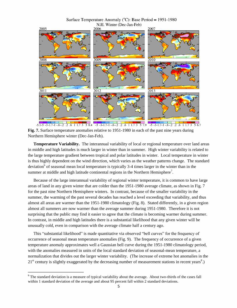
Fig. 7. Surface temperature anomalies relative to 1951-1980 in each of the past nine years during

Northern Hemisphere winter (Dec-Jan-Feb).

Temperature Variability. The interannual variability of local or regional temperature over land areas

in middle and high latitudes is much larger in winter than in summer. High winter variability is related to

the large temperature gradient between tropical and polar latitudes in winter. Local temperature in winter

is thus highly dependent on the wind direction, which varies as the weather patterns change. The standard

deviationb of seasonal mean local temperature is typically 3-4 times larger in the winter than in the

summer at middle and high latitude continental regions in the Northern Hemisphere7.

Because of the large interannual variability of regional winter temperature, it is common to have large

areas of land in any given winter that are colder than the 1951-1980 average climate, as shown in Fig. 7

for the past nine Northern Hemisphere winters. In contrast, because of the smaller variability in the

summer, the warming of the past several decades has reached a level exceeding that variability, and thus

almost all areas are warmer than the 1951-1980 climatology (Fig. 8). Stated differently, in a given region

almost all summers are now warmer than the average summer during 1951-1980. Therefore it is not

surprising that the public may find it easier to agree that the climate is becoming warmer during summer.

In contrast, in middle and high latitudes there is a substantial likelihood that any given winter will be

unusually cold, even in comparison with the average climate half a century ago.

This “substantial likelihood” is made quantitative via observed “bell curves” for the frequency of

occurrence of seasonal mean temperature anomalies (Fig. 9). The frequency of occurrence of a given

temperature anomaly approximates well a Gaussian bell curve during the 1951-1980 climatology period,

with the anomalies measured in units of the local standard deviation of seasonal-mean temperature, a

normalization that divides out the larger winter variability. (The increase of extreme hot anomalies in the

21st century is slightly exaggerated by the decreasing number of measurement stations in recent years

8.)

b The standard deviation is a measure of typical variability about the average. About two-thirds of the cases fall

within 1 standard deviation of the average and about 95 percent fall within 2 standard deviations.

6

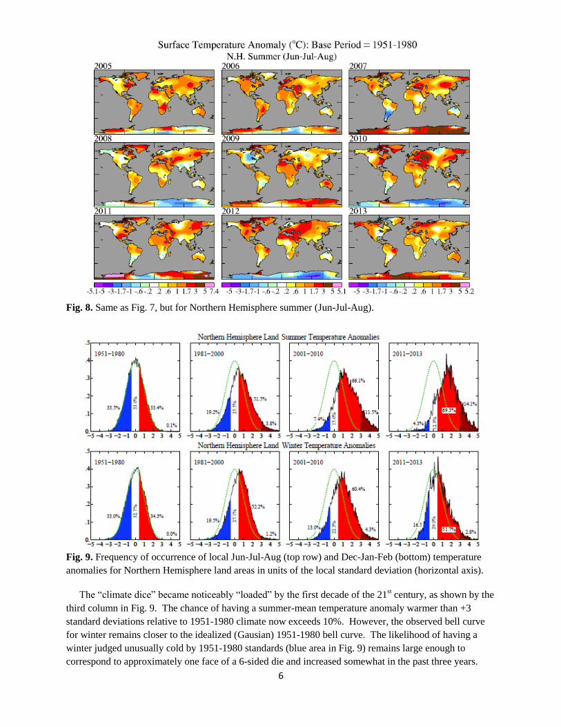
Fig. 8. Same as Fig. 7, but for Northern Hemisphere summer (Jun-Jul-Aug).

Fig. 9. Frequency of occurrence of local Jun-Jul-Aug (top row) and Dec-Jan-Feb (bottom) temperature

anomalies for Northern Hemisphere land areas in units of the local standard deviation (horizontal axis).

The “climate dice” became noticeably “loaded” by the first decade of the 21st century, as shown by the

third column in Fig. 9. The chance of having a summer-mean temperature anomaly warmer than +3

standard deviations relative to 1951-1980 climate now exceeds 10%. However, the observed bell curve

for winter remains closer to the idealized (Gausian) 1951-1980 bell curve. The likelihood of having a

winter judged unusually cold by 1951-1980 standards (blue area in Fig. 9) remains large enough to

correspond to approximately one face of a 6-sided die and increased somewhat in the past three years.

7

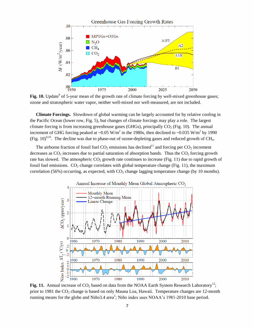
Fig. 10. Update

9 of 5-year mean of the growth rate of climate forcing by well-mixed greenhouse gases;

ozone and stratospheric water vapor, neither well-mixed nor well-measured, are not included.

Climate Forcings. Slowdown of global warming can be largely accounted for by relative cooling in

the Pacific Ocean (lower row, Fig. 5), but changes of climate forcings may play a role. The largest

climate forcing is from increasing greenhouse gases (GHGs), principally CO2 (Fig. 10). The annual

increment of GHG forcing peaked at ~0.05 W/m2 in the 1980s, then declined to ~0.035 W/m

2 by 1990

(Fig. 10)9,10

. The decline was due to phase-out of ozone-depleting gases and reduced growth of CH4.

The airborne fraction of fossil fuel CO2 emissions has declined11

and forcing per CO2 increment

decreases as CO2 increases due to partial saturation of absorption bands. Thus the CO2 forcing growth

rate has slowed. The atmospheric CO2 growth rate continues to increase (Fig. 11) due to rapid growth of

fossil fuel emissions. CO2 change correlates with global temperature change (Fig. 11), the maximum

correlation (56%) occurring, as expected, with CO2 change lagging temperature change (by 10 months).

Fig. 11. Annual increase of CO2 based on data from the NOAA Earth System Research Laboratory

12;

prior to 1981 the CO2 change is based on only Mauna Loa, Hawaii. Temperature changes are 12-month

running means for the globe and Niño3.4 area1; Niño index uses NOAA’s 1981-2010 base period.

8

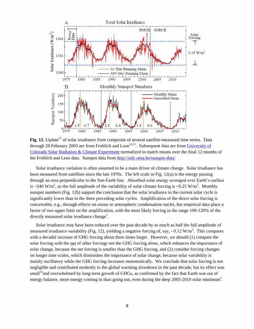
Fig. 12. Update

13 of solar irradiance from composite of several satellite-measured time series. Data

through 28 February 2003 are from Frohlich and Lean14,15

. Subsequent data are from University of

Colorado Solar Radiation & Climate Experiment normalized to match means over the final 12 months of

the Frohlich and Lean data. Sunspot data from http://sidc.oma.be/sunspot-data/

Solar irradiance variation is often assumed to be a main driver of climate change. Solar irradiance has

been measured from satellites since the late 1970s. The left scale in Fig. 12(a) is the energy passing

through an area perpendicular to the Sun-Earth line. Absorbed solar energy averaged over Earth’s surface

is ~240 W/m2, so the full amplitude of the variability of solar climate forcing is ~0.25 W/m

2. Monthly

sunspot numbers (Fig. 12b) support the conclusion that the solar irradiance in the current solar cycle is

significantly lower than in the three preceding solar cycles. Amplification of the direct solar forcing is

conceivable, e.g., through effects on ozone or atmospheric condensation nuclei, but empirical data place a

factor of two upper limit on the amplification, with the most likely forcing in the range 100-120% of the

directly measured solar irradiance change5.

Solar irradiance may have been reduced over the past decade by as much as half the full amplitude of

measured irradiance variability (Fig. 12), yielding a negative forcing of, say, - 0.12 W/m2. This compares

with a decadal increase of GHG forcing about three times larger. However, we should (1) compare the

solar forcing with the net of other forcings not the GHG forcing alone, which enhances the importance of

solar change, because the net forcing is smaller than the GHG forcing, and (2) consider forcing changes

on longer time scales, which diminishes the importance of solar change, because solar variability is

mainly oscillatory while the GHG forcing increases monotonically. We conclude that solar forcing is not

negligible and contributed modestly to the global warming slowdown in the past decade, but its effect was

small16

and overwhelmed by long-term growth of GHGs, as confirmed by the fact that Earth was out of

energy balance, more energy coming in than going out, even during the deep 2005-2010 solar minimum5.

9

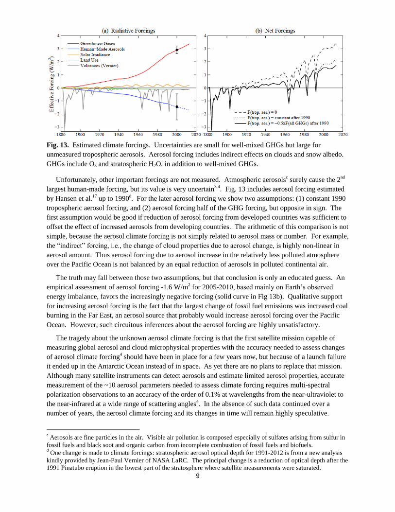
Fig. 13. Estimated climate forcings. Uncertainties are small for well-mixed GHGs but large for

unmeasured tropospheric aerosols. Aerosol forcing includes indirect effects on clouds and snow albedo.

GHGs include O3 and stratospheric H2O, in addition to well-mixed GHGs.

Unfortunately, other important forcings are not measured. Atmospheric aerosolsc surely cause the 2

nd

largest human-made forcing, but its value is very uncertain3,4

. Fig. 13 includes aerosol forcing estimated

by Hansen et al.17

up to 1990d. For the later aerosol forcing we show two assumptions: (1) constant 1990

tropospheric aerosol forcing, and (2) aerosol forcing half of the GHG forcing, but opposite in sign. The

first assumption would be good if reduction of aerosol forcing from developed countries was sufficient to

offset the effect of increased aerosols from developing countries. The arithmetic of this comparison is not

simple, because the aerosol climate forcing is not simply related to aerosol mass or number. For example,

the “indirect” forcing, i.e., the change of cloud properties due to aerosol change, is highly non-linear in

aerosol amount. Thus aerosol forcing due to aerosol increase in the relatively less polluted atmosphere

over the Pacific Ocean is not balanced by an equal reduction of aerosols in polluted continental air.

The truth may fall between those two assumptions, but that conclusion is only an educated guess. An

empirical assessment of aerosol forcing -1.6 W/m2 for 2005-2010, based mainly on Earth’s observed

energy imbalance, favors the increasingly negative forcing (solid curve in Fig 13b). Qualitative support

for increasing aerosol forcing is the fact that the largest change of fossil fuel emissions was increased coal

burning in the Far East, an aerosol source that probably would increase aerosol forcing over the Pacific

Ocean. However, such circuitous inferences about the aerosol forcing are highly unsatisfactory.

The tragedy about the unknown aerosol climate forcing is that the first satellite mission capable of

measuring global aerosol and cloud microphysical properties with the accuracy needed to assess changes

of aerosol climate forcing4 should have been in place for a few years now, but because of a launch failure

it ended up in the Antarctic Ocean instead of in space. As yet there are no plans to replace that mission.

Although many satellite instruments can detect aerosols and estimate limited aerosol properties, accurate

measurement of the ~10 aerosol parameters needed to assess climate forcing requires multi-spectral

polarization observations to an accuracy of the order of 0.1% at wavelengths from the near-ultraviolet to

the near-infrared at a wide range of scattering angles4. In the absence of such data continued over a

number of years, the aerosol climate forcing and its changes in time will remain highly speculative.

c Aerosols are fine particles in the air. Visible air pollution is composed especially of sulfates arising from sulfur in

fossil fuels and black soot and organic carbon from incomplete combustion of fossil fuels and biofuels. d One change is made to climate forcings: stratospheric aerosol optical depth for 1991-2012 is from a new analysis

kindly provided by Jean-Paul Vernier of NASA LaRC. The principal change is a reduction of optical depth after the

1991 Pinatubo eruption in the lowest part of the stratosphere where satellite measurements were saturated.

10

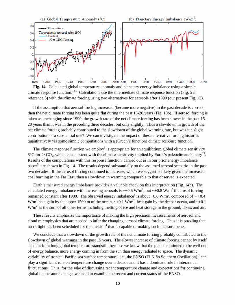
Fig. 14. Calculated global temperature anomaly and planetary energy imbalance using a simple

climate response function.18,5

Calculations use the intermediate climate response function (Fig. 5 in

reference 5) with the climate forcing using two alternatives for aerosols after 1990 (our present Fig. 13).

If the assumption that aerosol forcing increased (became more negative) in the past decade is correct,

then the net climate forcing has been quite flat during the past 15-20 years (Fig. 13b). If aerosol forcing is

taken as unchanging since 1990, the growth rate of the net climate forcing has been slower in the past 15-

20 years than it was in the preceding three decades, but only slightly. Thus a slowdown in growth of the

net climate forcing probably contributed to the slowdown of the global warming rate, but was it a slight

contribution or a substantial one? We can investigate the impact of these alternative forcing histories

quantitatively via some simple computations with a (Green’s function) climate response function.

The climate response function we employ5 is appropriate for an equilibrium global climate sensitivity

3°C for 2×CO2, which is consistent with the climate sensitivity implied by Earth’s paleoclimate history19

.

Results of the computations with this response function, carried out as in our prior energy imbalance

paper5, are shown in Fig. 14. The results depend substantially on the assumed aerosol scenario in the past

two decades. If the aerosol forcing continued to increase, which we suggest is likely given the increased

coal burning in the Far East, then a slowdown in warming comparable to that observed is expected.

Earth’s measured energy imbalance provides a valuable check on this interpretation (Fig. 14b). The

calculated energy imbalance with increasing aerosols is ~+0.6 W/m2, but ~+0.8 W/m

2 if aerosol forcing

remained constant after 1990. The observed energy imbalance5 is about +0.6 W/m

2, composed of ~+0.4

W/m2 heat gain by the upper 1500 m of the ocean, ~+0.1 W/m

2, heat gain by the deeper ocean, and ~+0.1

W/m2 as the sum of all other terms including melting of ice and heat storage in the ground, lakes, and air.

These results emphasize the importance of making the high precision measurements of aerosol and

cloud microphysics that are needed to infer the changing aerosol climate forcing. Thus it is puzzling that

no reflight has been scheduled for the mission4 that is capable of making such measurements.

We conclude that a slowdown of the growth rate of the net climate forcing probably contributed to the

slowdown of global warming in the past 15 years. The slower increase of climate forcing cannot by itself

account for a long global temperature standstill, because we know that the planet continued to be well out

of energy balance, more energy coming in from the sun than energy radiated to space. The dynamic

variability of tropical Pacific sea surface temperature, i.e., the ENSO (El Niño Southern Oscillation),2 can

play a significant role on temperature change over a decade and it has a dominant role in interannual

fluctuations. Thus, for the sake of discussing recent temperature change and expectations for continuing

global temperature change, we need to examine the recent and current status of the ENSO.

11

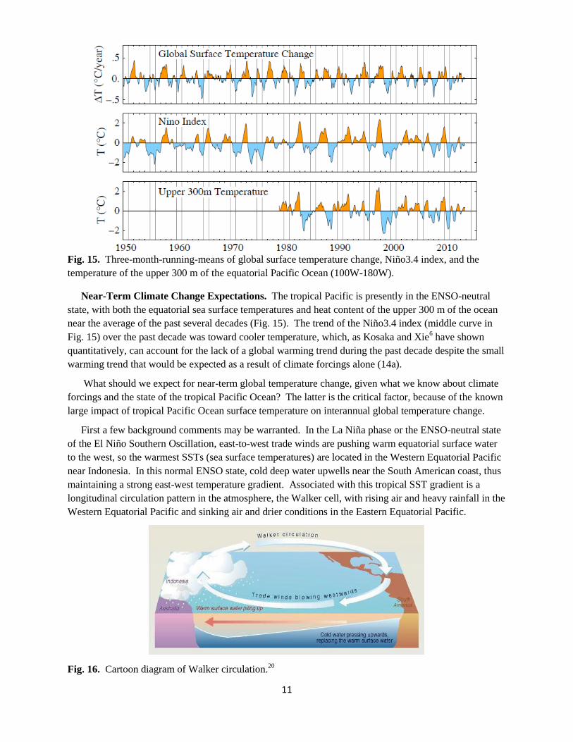
Fig. 15. Three-month-running-means of global surface temperature change, Niño3.4 index, and the

temperature of the upper 300 m of the equatorial Pacific Ocean (100W-180W).

Near-Term Climate Change Expectations. The tropical Pacific is presently in the ENSO-neutral

state, with both the equatorial sea surface temperatures and heat content of the upper 300 m of the ocean

near the average of the past several decades (Fig. 15). The trend of the Niño3.4 index (middle curve in

Fig. 15) over the past decade was toward cooler temperature, which, as Kosaka and Xie6 have shown

quantitatively, can account for the lack of a global warming trend during the past decade despite the small

warming trend that would be expected as a result of climate forcings alone (14a).

What should we expect for near-term global temperature change, given what we know about climate

forcings and the state of the tropical Pacific Ocean? The latter is the critical factor, because of the known

large impact of tropical Pacific Ocean surface temperature on interannual global temperature change.

First a few background comments may be warranted. In the La Niña phase or the ENSO-neutral state

of the El Niño Southern Oscillation, east-to-west trade winds are pushing warm equatorial surface water

to the west, so the warmest SSTs (sea surface temperatures) are located in the Western Equatorial Pacific

near Indonesia. In this normal ENSO state, cold deep water upwells near the South American coast, thus

maintaining a strong east-west temperature gradient. Associated with this tropical SST gradient is a

longitudinal circulation pattern in the atmosphere, the Walker cell, with rising air and heavy rainfall in the

Western Equatorial Pacific and sinking air and drier conditions in the Eastern Equatorial Pacific.

Fig. 16. Cartoon diagram of Walker circulation.20

12

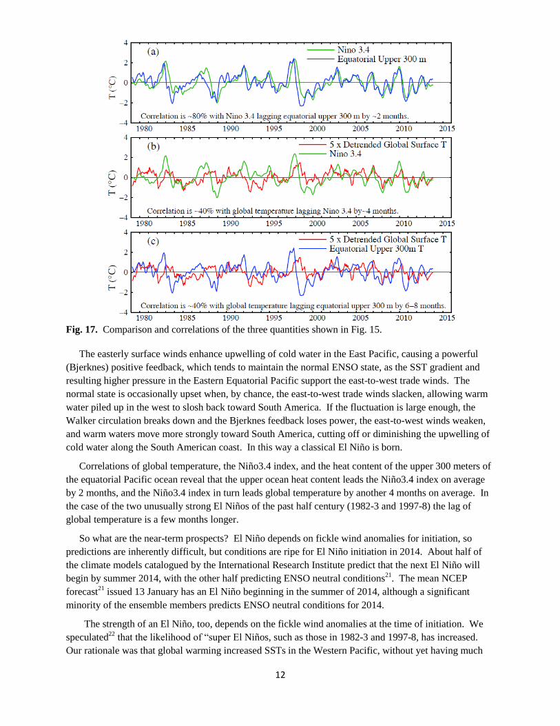
Fig. 17. Comparison and correlations of the three quantities shown in Fig. 15.

The easterly surface winds enhance upwelling of cold water in the East Pacific, causing a powerful

(Bjerknes) positive feedback, which tends to maintain the normal ENSO state, as the SST gradient and

resulting higher pressure in the Eastern Equatorial Pacific support the east-to-west trade winds. The

normal state is occasionally upset when, by chance, the east-to-west trade winds slacken, allowing warm

water piled up in the west to slosh back toward South America. If the fluctuation is large enough, the

Walker circulation breaks down and the Bjerknes feedback loses power, the east-to-west winds weaken,

and warm waters move more strongly toward South America, cutting off or diminishing the upwelling of

cold water along the South American coast. In this way a classical El Niño is born.

Correlations of global temperature, the Niño3.4 index, and the heat content of the upper 300 meters of

the equatorial Pacific ocean reveal that the upper ocean heat content leads the Niño3.4 index on average

by 2 months, and the Niño3.4 index in turn leads global temperature by another 4 months on average. In

the case of the two unusually strong El Niños of the past half century (1982-3 and 1997-8) the lag of

global temperature is a few months longer.

So what are the near-term prospects? El Niño depends on fickle wind anomalies for initiation, so

predictions are inherently difficult, but conditions are ripe for El Niño initiation in 2014. About half of

the climate models catalogued by the International Research Institute predict that the next El Niño will

begin by summer 2014, with the other half predicting ENSO neutral conditions21

. The mean NCEP

forecast21

issued 13 January has an El Niño beginning in the summer of 2014, although a significant

minority of the ensemble members predicts ENSO neutral conditions for 2014.

The strength of an El Niño, too, depends on the fickle wind anomalies at the time of initiation. We

speculated22

that the likelihood of “super El Niños, such as those in 1982-3 and 1997-8, has increased.

Our rationale was that global warming increased SSTs in the Western Pacific, without yet having much

13

effect on the temperature of upwelling deep water in the Eastern Pacific (Fig. 2 above), thus allowing the

possibility of a larger swing of Eastern Pacific temperature. Recent paleoclimate23

and modeling24

studies

find evidence for an increased frequency of extreme El Niños with global warming.

Assuming that an El Niño begins in summer 2014, 2014 is likely to be warmer than 2013 and perhaps

the warmest year in the instrumental record. However, given the lag between El Niño initiation and

global temperature, 2015 is likely to have a temperature even higher than in 2014.

Summary. The recent slowdown of global warming is a consequence of both a slowdown in the

growth rate of climate forcings and recent ENSO history. Given that the tropical Pacific seems to be

moving toward the next El Niño, record global temperature is likely in the near term. However, the rate

of future warming will depend upon changes of the tropospheric aerosol forcing, which is highly

uncertain and unmeasured.

Acknowledgments. We thank Gavin Schmidt for comments on the draft manuscript.

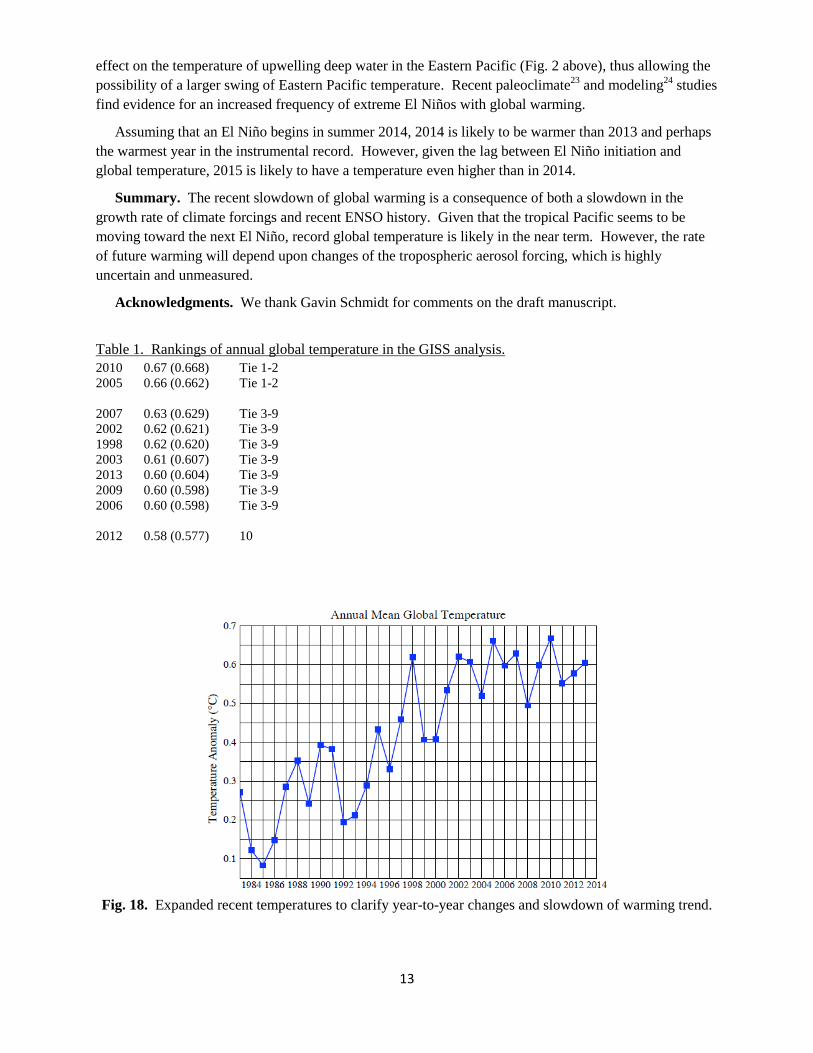
Table 1. Rankings of annual global temperature in the GISS analysis.

2010 0.67 (0.668) Tie 1-2

2005 0.66 (0.662) Tie 1-2

2007 0.63 (0.629) Tie 3-9

2002 0.62 (0.621) Tie 3-9

1998 0.62 (0.620) Tie 3-9

2003 0.61 (0.607) Tie 3-9

2013 0.60 (0.604) Tie 3-9

2009 0.60 (0.598) Tie 3-9

2006 0.60 (0.598) Tie 3-9

2012 0.58 (0.577) 10

Fig. 18. Expanded recent temperatures to clarify year-to-year changes and slowdown of warming trend.

14

References

1 Hansen, J., R. Ruedy, M. Sato, and K. Lo, 2010: Global surface temperature change. Rev. Geophys., 48, RG4004,

doi:10.1029/2010RG000345. 2 Philander, S.G., Our Affair with El Niño: How We Transformed an Enchanting Peruvian Current into a Global

Climate Hazard, Princeton Univ. Press, Princeton, NJ, 288 pp., 2006. 3 Intergovernmental Panel on Climate Change, Climate Change 2007: The Physical Science Basis, eds. S. Solomon,

et al., Cambridge Univ. Press, New York, 2007. 4 Mishchenko, M.I., B. Cairns, G. Kopp, C.F. Schueler, B.A. Fafaul, J.E. Hansen, R.J. Hooker, T. Itchkawich, H.B.

Maring, and L.D. Travis, 2007: Accurate monitoring of terrestrial aerosols and total solar irradiance: Introducing the

Glory mission. Bull. Amer. Meteorol. Soc., 88, 677-691, doi:10.1175/BAMS-88-5-677. 5 Hansen, J., M. Sato, P. Kharecha, and K. von Schuckmann, 2011: Earth's energy imbalance and implications.

Atmos. Chem. Phys., 11, 13421-13449, doi:10.5194/acp-11-13421-2011. 6 Kosaka, Y., Xie, S.P., Recent global warming hiatus tied to equatorial Pacific surface cooling, Nature 501, 403-

407, 2013, doi:10.1038/nature12534 7 Hansen, J., M. Sato, and R. Ruedy, 2012: Perception of climate change. Proc. Natl. Acad. Sci., 109, 14726-14727,

E2415-E2423, doi:10.1073/pnas.1205276109. 8 Hansen, J., M. Sato, and R. Reudy, 2013: Reply to Rhines and Huybers: Changes in the frequency of extreme

summer heat. Proc. Natl. Acad. Sci., 110, E547-E548, doi:10.1073/pnas.1220916110. 9 Hansen, J., and M. Sato, 2004: Greenhouse gas growth rates. Proc. Natl. Acad. Sci., 101, 16109-16114,

doi:10.1073/pnas.0406982101. 10

Hansen, J., M. Sato, R. Ruedy, A. Lacis, and V. Oinas, 2000: Global warming in the twenty-first century: An

alternative scenario. Proc. Natl. Acad. Sci., 97, 9875-9880, doi:10.1073/pnas.170278997. 11

Hansen, J., P. Kharecha, and M. Sato, 2013: Climate forcing growth rates: Doubling down on our Faustian

bargain. Environ. Res. Lett., 8, 011006, doi:10.1088/1748-9326/8/1/011006. 12

Earth System Research Laboratory (2013) www.esrl.noaa.gov/gmd/ccgg/trends/ 13

Hansen, J., P. Kharecha, M. Sato, V. Masson-Delmotte, F. Ackerman, D. Beerling, P.J. Hearty, O. Hoegh-

Guldberg, S.-L. Hsu, C. Parmesan, J. Rockstrom, E.J. Rohling, J. Sachs, P. Smith, K. Steffen, L. Van Susteren, K.

von Schuckmann, and J.C. Zachos, 2013: Assessing "dangerous climate change": Required reduction of carbon

emissions to protect young people, future generations and nature. PLOS ONE, 8, e81648,

doi:10.1371/journal.pone.0081648. 14

Frohlich C., J. Lean, 1998: The Sun's total irradiance: cycles and trends in the past two decades and associated

climate change uncertainties. Geophys. Res. Lett. 25, 4377-4380. 15

Physikalisch Meteorologisches Observatorium Davos, World Radiation Center 16

Meehl G.A., J.M. Arblaster, D.R. Marsh, 2013: Could a future "Grand Solar Minimum" like the Maunder

Minimum stop global warming? Geophys Res Lett 40, 1789-1793. 17

Hansen, J., M. Sato, R. Ruedy, P. Kharecha, A. Lacis, R.L. Miller, L. Nazarenko, K. Lo, G.A. Schmidt, G.

Russell, I. et al., 2007: Dangerous human-made interference with climate: A GISS modelE study. Atmos. Chem.

Phys., 7, 2287-2312, doi:10.5194/acp-7-2287-2007. 18

Hansen, J., 2008: Climate threat to the planet: implications for energy policy and intergenerational justice,

Bjerknes lecture, American Geophysical Union, San Francisco, 17 December, available at:

www.columbia.edu/~jeh1/presentations.shtml, 2008. 19

Hansen, J., M. Sato, G. Russell, and P. Kharecha, 2013: Climate sensitivity, sea level, and atmospheric carbon

dioxide. Phil. Trans. R. Soc. A, 371, 20120294, doi:10.1098/rsta.2012.0294. 20

www.google.com/search?q=walker+circulation&tbm=isch&tbo=u&source=univ&sa=X&ei=bU_dUsDYBPSvsQTb2oCYDw&sqi=2&ved=0CDYQsAQ&biw=1600&bih=713

21 http://www.cpc.ncep.noaa.gov/products/precip/CWlink/MJO/enso.shtml#discussion 22

Hansen, J., M. Sato, R. Ruedy, K. Lo, D.W. Lea, and M. Medina-Elizade, 2006: Global temperature change. Proc.

Natl. Acad. Sci., 103, 14288-14293, doi:10.1073/pnas.0606291103. 23

McGregor, S., A. Timmermann, M.H. England, O.E. Timm, A.T. Wittenberg, 2013: Inferred changes in El Niño-

Southern Oscillation variance over the past six centuries. Clim. Past 9, 2269-2284. 24

Cai, W. and 13 co-aluthors, 2014: Increasing frequency of extreme El Niño events due to greenhouse warming.

Nature Clim. Change, publ. on-line 19 January 2014 doi:10.1038/NCLIMATE2100