Embed Size (px)
Citation preview

Banco de Mexico
Documentos de Investigacion
Banco de Mexico
Working Papers
N 2004-06
Globalization, Regional Wage Differentialsand the Stolper-Samuelson Theorem:
Evidence from Mexico
Daniel ChiquiarBanco de Mexico
October 2004
La serie de Documentos de Investigacion del Banco de Mexico divulga resultados preliminares detrabajos de investigacion economica realizados en el Banco de Mexico con la finalidad de propiciarel intercambio y debate de ideas. El contenido de los Documentos de Investigacion, ası como lasconclusiones que de ellos se derivan, son responsabilidad exclusiva de los autores y no reflejannecesariamente las del Banco de Mexico.
The Working Papers series of Banco de Mexico disseminates preliminary results of economicresearch conducted at Banco de Mexico in order to promote the exchange and debate of ideas. Theviews and conclusions presented in the Working Papers are exclusively the responsibility of theauthors and do not necessarily reflect those of Banco de Mexico.

Documento de Investigacion Working Paper2004-06 2004-06
Globalization, Regional Wage Differentials and theStolper-Samuelson Theorem: Evidence from Mexico1
Daniel Chiquiar 2
Banco de Mexico
AbstractUsing individual-level data on personal characteristics and wages and state-level data on
trade, foreign direct investment, international migration and other site-specific features, Istudy what factors determined the changes in Mexico’s regional wage differentials between1990 and 2000. I exploit the regional variation in the exposure to globalization to identifythe effects of NAFTA on wages and on returns to schooling. The results support the presenceof Stolper-Samuelson type of responses during Mexico’s globalization process: regions moreexposed to international markets appear to have exhibited an increase in wage levels, but adecrease in returns to schooling, relative to other regions of the country. The results suggestthat globalization has an important spatial dimension that is usually neglected in traditionaltrade models.
Keywords: Trade Liberalization, Stolper-Samuelson Theorem, Wage Differentials, NAF-TA, Economic Geography.JEL Classification: F11, F14, F16
ResumenEn este trabajo se analizan los factores que influyeron en los cambios de los diferenciales
salariales regionales en Mexico durante la decada de los 90’s. Se explota la variacion regio-nal en el grado de integracion con los mercados internacionales para identificar los efectosdel TLCAN sobre los salarios y los rendimientos a la educacion. Los resultados apoyan lahipotesis de que existieron respuestas tipo Stolper-Samuelson en los precios de los factoresante la apertura comercial. En particular, las regiones mas expuestas a los mercados inter-nacionales tendieron a exhibir un aumento en los niveles salariales, pero una disminucion enlos rendimientos a la educacion, en comparacion con el resto del paıs.
Palabras Clave: Liberalizacion Comercial, Teorema Stolper-Samuelson, Diferenciales Salaria-les, TLCAN, Geografıa Economica.
1I thank Kate Antonovics, Julian Betts, Richard Carson, Susana Ferreira, Rodrigo Garcıa-Verdu,Theodore Groves, Gordon Hanson, Mark Machina, James Rauch, and Chris Woodruff for very helpful com-ments and the Consejo Nacional de Ciencia y Tecnologıa (CONACYT) for financial support.
2Direccion General de Investigacion Economica. Email: [email protected].

1
1. Introduction
The debate concerning the sources of the increase in wage inequality within developed
countries from the eighties on remains to be resolved. Some observers have attributed the rise
in skill premiums to the current globalization process, in which many less developed, unskilled
labor abundant countries have become integrated to international goods and capital flows
(Leamer, 1993 and 1994; Wood, 1994 and 1995; Sachs and Shatz, 1996). Others have argued
that technological progress, and not trade, is the main culprit of increasing inequality within
developed countries (Lawrence and Slaughter, 1993; Berman, Bound and Griliches, 1994;
Baldwin and Cain, 1997).1
Some existing evidence suggests that wage inequality has also increased within less
developed countries that liberalized to trade in this period (Cragg and Epelbaum, 1996; Davis,
1996; Feenstra and Hanson, 1997; Revenga and Montenegro, 1998). This only compounds the
difficulty in resolving the debate: if trade is the main culprit of the increase in inequality within
the developed world, then under a Heckscher-Ohlin framework we should have expected a
simultaneous decrease in developing countries’ skill premiums. The fact that this apparently
didn’t happen may appear to be evidence against the view that trade is the main cause of rising
inequality. However, some authors have modified the basic Heckscher-Ohlin framework to
account for some recent trends in the globalization process (the regional disintegration of
production, the increased role of multinationals, etc.) and have concluded that trade may indeed
be behind the rise in skill premiums in both developed and less developed countries (Feenstra
and Hanson, 1996; Markusen and Zahnizer, 1997; Feenstra, 1998). The evidence from less
developed countries, therefore, has not been able to solve the debate in any direction.
Mexico’s experience is an excellent case to study the links between globalization and
wages. Mexico opened-up to trade unilaterally and signed on to the General Agreement on

2
Tariffs and Trade (GATT) in 1986. A second stage in its liberalization process can be
identified with the enactment of the North American Free Trade Agreement (NAFTA), which
started operating in 1994. The second stage of Mexico’s globalization locked-in the unilateral
opening-up conducted during the first stage and deepened Mexico’s integration with the U.S.
in terms of trade in goods and capital flows. An analysis of the effects of NAFTA on Mexico’s
input prices could yield relevant insights concerning the links between globalization and wage
inequality and provide useful evidence to test the predictive power of the Stolper-Samuelson
Theorem in a context of increasing economic integration between skill abundant and skill
scarce economies.
In this context, the existing evidence has been unable to find strong support for the
presence of Stolper-Samuelson type of responses in Mexico’s input prices after its
globalization. Indeed, a strong increase in the skill premium was observed after the first stage
of Mexico’s trade liberalization. As a consequence, the debate concerning the role of trade in
the increase in wage inequality has been recreated within the group of analysts that study
Mexico’s globalization experience: some argue that the evolution of relative wages in Mexico
has not been a result of trade, while others have developed alternative trade models implying
that globalization may indeed be behind the rise in Mexico’s skill premium.
There are some shortcomings in the existing literature that may explain why a Stolper-
Samuelson response has not been identified for Mexico’s input prices. First, most of the
literature is based only on the first stage of Mexico’s liberalization. It is during the second
stage of Mexico’s globalization when this country strengthened its links specifically with skill-
abundant countries and the Stolper-Samuelson Theorem would unambiguously predict a
decrease in the skill premium. Second, not all regions within Mexico are equally linked to the
international economy. In this context, the response of input prices to trade liberalization may
1 Surveys on the wage inequality debate may be found in Freeman (1995) and Richardson (1995). A critical

3
have been regionally heterogeneous, making it difficult to identify Stolper-Samuelson kind of
responses using economy-wide data. There has been no attempts, however, to exploit regional
variations in the degree of exposure to international markets to identify these effects.
In this paper, I address these issues by assessing empirically what were the forces that
contributed to the changes in wage differentials across Mexico’s regions during the nineties
and by using the regional variation in the degree of exposure to international markets to
identify the effects of the second stage of Mexico’s opening up on wages and on returns to
schooling. This allows assessing to what extent Mexico’s globalization experience yielded
results consistent with the predictions of the Heckscher-Ohlin model.
The fundamental conclusion that emerges from this paper is that Mexico’s experience
with globalization, at least during the second stage of its reforms, appears to be consistent with
the Stolper-Samuelson Theorem. Overall wages in general, and unskilled wages in particular,
increased in regions that exhibit stronger links with the U.S. market, as compared to regions
that do not exhibit such an integration with the U.S. This is, the broader integration of these
specific regions with a more skill-abundant country apparently led to an increase in their
overall wages, but a decline in their skill premium, as compared to the rest of the country. In
this context, the nation-wide rise in the skill premium observed after Mexico’s globalization
may have been a response to factors unrelated to trade.
While wages in regions more exposed to international markets behaved as traditional
trade models would predict, the results of this paper suggest the existence of a distinct, spatial
dimension in the effects of globalization on wages that is usually neglected in traditional
models. Wage differentials between regions close to the U.S. border and the rest of the country,
for similar individuals, tended to increase during the nineties. As a consequence, workers with
similar characteristics fared differently in response to Mexico’s trade liberalization depending
review is found in Krugman (1995).

4
on their geographical location. In this context, the results of this paper are consistent with the
new economic-geography type of arguments that have been set forth to account for Mexico’s
experience with trade liberalization. I therefore conclude that globalization of a skill-scarce
country may lead to increases in wage inequality, once its spatial dimension is taken into
account.
The rest of the paper is divided as follows. In Section 2 I briefly review the current
literature concerning the effect of Mexico’s globalization on regional wages and the skill
premium, and expose some of the shortcomings of this literature. Section 3 describes the basic
regional differences across Mexico in terms of labor force characteristics and the influence of
globalization. Section 4 presents a theoretical model that suggests that spatial considerations
may be important when addressing the effects of globalization on domestic input prices.
Section 5 estimates individual-level wage equations and analyzes the regional implications of
the results. It also describes an econometric exercise in which the regional differences in
exposure to international markets are used to identify the effects of globalization on the wage-
schooling profile. Finally, Section 6 summarizes the main results.
2. Regional Wage Differentials and the Skill Premium During Mexico’s Globalization
Coinciding with Mexico’s globalization, a process of divergence in regional wages has
been observed. Since the mid-eighties, wage differentials across Mexico’s regions tended to
widen: wage levels in sites closer to the U.S. border increased substantially as compared to the
rest of the country, in general, and to Mexico City, in particular.2 Using economic-geography
type of models, the literature has suggested that the regional employment, wage and per capita
2 A similar behavior was observed in terms of per capita output levels. The convergent pattern in regional per capita GDP levels observed before 1985 apparently broke down after the trade reforms, as a consequence of the fact that the initially richer regions (Mexico City and the border and northern states) exhibited higher growth rates than other regions of the country (Juan-Ramón and Rivera-Bátiz, 1996; Messmacher, 2000; García-Verdú, 2002; Esquivel and Messmacher, 2002; Rodríguez-Pose and Sánchez-Reaza, 2002; and Chiquiar, 2003).

5
GDP patterns observed during this period were a consequence of Mexico’s globalization.
According to this literature, the trade reforms altered the optimal location choice of
manufacturing firms, promoting the break-up of Mexico City’s manufacturing belt and a
movement of economic activity towards the border with the U.S. (Krugman and Livas
Elizondo, 1996; Hanson, 1996, 1997, 1998a and 1998b; Katz, 1998; Dávila, Kessel and Levy,
2002; Meardon, 2003).3 According to these authors, the relative increase in the market
potential of firms located near the U.S. led to an increase in border wages, as compared to the
wages observed in the rest of the country and, in particular, in Mexico City.
Consistently with the literature cited above, after the trade reforms Mexico City’s share
of manufacturing employment declined substantially, while the share corresponding to the
states that have a border with the U.S. rose steadily (see Figure 1). Large foreign-owned,
export-oriented plants and, in particular, maquiladoras, account for most of the manufacturing
employment growth observed after NAFTA was enacted (López-Córdova, 2001). These plants
are heavily concentrated in the border region.4 This suggests that the increase in manufacturing
exports may have had a disproportionately large effect on employment, wages and growth in
that region, and only small effects in the center and south of the country.
Although there seems to be consensus regarding the factors behind the regional
behavior of employment, output and wages after Mexico opened up to trade, the existing
evidence has been unable to find strong support for the presence of Stolper-Samuelson type of
3 Another mechanism through which the trade reforms had a heterogeneous impact across Mexico’s regions is related to the fact that agricultural producers in the north use modern technologies and irrigated land to produce fruits and vegetables for which Mexico holds a comparative advantage, while southern peasants are concentrated in subsistence agriculture based on traditional techniques and rain-fed land. The reciprocal dismantling of protection devices implied by NAFTA boosted exports of northern agricultural products to the U.S., at the same time that southern producers were hit by the elimination of protection on the products they produce (see Brown, Deardorff and Stern, 1992; Levy and Van Wijnbergen, 1995; Lustig, 2001; and Veeman, Veeman and Hoskins, 2002). 4 Mexico allowed the creation of foreign owned maquiladora assembly plants with a duty-free treatment since the mid-sixties. These plants import virtually all raw materials from the U.S., use Mexican labor force to conduct assembly activities, and export the processed product back to the U.S. The program was originally instrumented to avoid unemployment problems in the border derived from the return of Mexican workers in the U.S. after the Bracero program was dismantled.

6
mechanisms in Mexico’s response to globalization. Indeed, a strong increase in the relative
wage of skilled workers was observed after the first stage of Mexico’s globalization. This event
broke down the gradual decline in the skilled-unskilled wage gap that was observed up to
1985. If we assume that Mexico has a relative abundance of unskilled labor, this behavior
seems to be inconsistent with the Stolper-Samuelson Theorem.
This puzzle has led some authors to argue that the evolution of relative wages has not
been a result of trade, but of skill-biased technological change or of an increase in the relative
demand for skilled workers derived from domestic reforms (Cragg and Epelbaum, 1996;
Robertson, 2000b; Alvarez and Robertson, 2001; Airola, 2001; and Melendez, 2001). Others
have extended traditional trade models to take into account that the main outcome of Mexico’s
liberalization was to induce its firms to specialize in assembly activities and become part of
global production networks. For example, Feenstra and Hanson (1996 and 1997) develop a
model that suggests that, as U.S. firms increase purchases of inputs from Mexican firms or set
up assembly firms within Mexican territory, the skill premium increases in both countries.
They provide evidence showing that foreign direct investment growth in the form of
maquiladora plants may account for more than half of the increase in the skilled labor share in
wages observed in the border region during the late eighties. Markusen and Zahnizer (1997)
present a model based on the behavior of multinationals that has similar implications.
There are two issues concerning the existing literature that deserve further discussion.
First, most of the existing literature is based only on the first stage of Mexico’s liberalization.
As Robertson (2000a and 2001) points out, while Mexico has a comparative advantage in
unskilled labor-intensive goods with respect to the U.S., at the same time it may be more skill-
abundant than other less developed countries. Thus, during the first stage of its liberalization
process, Mexico may have faced enhanced competition from more unskilled-labor abundant

7
countries.5 It is during the second stage of Mexico’s globalization when this country
strengthened its links with clearly more skill-abundant countries and the Stolper-Samuelson
Theorem would unambiguously predict a decrease in the skill premium. With the benefit of
using more recent data, Robertson (2000a and 2001) provides evidence that, precisely after
NAFTA started operating, the increasing trend in the skill premium stopped and, in fact, this
premium started falling again (see Figure 2). Thus, the overall evolution of the skill premium
in Mexico may in fact be consistent with the predictions of the Stolper-Samuelson Theorem.
Second, not all regions within Mexico are equally linked to the international economy.
If inputs are not perfectly mobile across regions, then the response of input prices to trade
liberalization may have been regionally heterogeneous, making it difficult to identify Stolper-
Samuelson kind of responses using economy-wide data. Most of the existing literature,
however, has relied on the economy-wide variation in protection levels across industries to
assess the effect of Mexico’s globalization on wages. There has been no attempt so far to
exploit regional variations in the degree of exposure to international markets in order to
identify these effects.6
In the remainder of this paper, I address these issues explicitly. I focus on the second
stage of Mexico’s globalization process and I exploit the regional variation in the degree of
exposure to international markets to identify the effect of globalization on wages. In this
context, it is important to note that Mexico’s regions exhibit large differences in natural
resource endowments, infrastructure, past regional policies and historically-determined
5 This may give a rationale for the existing evidence suggesting that, just before the reforms, Mexico was protecting more heavily its most unskilled-labor intensive sectors (Hanson and Harrison, 1999). After the first stage of Mexico’s opening up, it was these sectors which exhibited largest decreases in protection levels. Moreover, the rents derived from protection were apparently shared with workers. Thus, as protection was dismantled, the earnings of unskilled workers may have fallen not only as the result of the reduction in these sectors’ labor demand, but also as a consequence of the reduction in available rents (see Revenga, 1997; and Revenga and Montenegro, 1998). 6 An exception is Airola (2001), who uses regional differences in maquiladora presence to identify the effects of globalization on the skill premium. He shows that, once post-NAFTA data are included in the analysis, the conclusions concerning the positive effect of foreign direct investment on the skill premium obtained by previous

8
agglomerations of population. The existence of site-specific features that, while unrelated to
Mexico’s trade reforms, may have also influenced Mexico’s regional wage patterns in the last
decades, render it difficult to identify the specific role that globalization had in the
determination of regional wage differentials within Mexico. In order to identify and test the
presence of Stolper-Samuelson type of effects, I make an explicit attempt to disentangle what
was the relative influence of geographic location and of other globalization-related effects on
the changes of regional wage differentials observed after Mexico’s opening up.
3. Data and Summary Statistics
In this section, I summarize the main differences across Mexico’s regions in terms of
the characteristics of their populations and their links with the international economy. In order
to conduct the analysis, I divide Mexico into 5 regions: i) states that have a border with the
U.S.; ii) the northern region, just below the border states; iii) the center region; iv) the capital
(Mexico City and its surroundings); and, v) the southern region (see Figure 3).
The data used correspond to 1% samples of male individuals taken from Mexico’s 1990
and 2000 population censuses.7 I complement this sample with state-level data on several site-
specific features and globalization-related measures, such as the presence of large firms,
tourism activity, migration rates, maquiladora employment, foreign direct investment flows,
and the distance from the largest city in each state to the closest major U.S. border crossing.
3.1. Individual Characteristics
Tables 1a and 1b summarize the demographic characteristics of 25-65 year old males in
1990 and in 2000, while Tables 2 and 3 summarize the distribution of each region’s 25-65 year
authors are overturned. While his findings are similar to those I report here, I use a broader set of globalization-related indicators.

9
old working male population by sector of employment, occupation and position in the job.
Large differences in the composition of the labor force and in the orientation of economic
activity across Mexico’s regions are observed. The labor force in Mexico City and the border
appears to be more educated and mostly urban and industry-oriented in nature, while working
individuals in the south represent a much less educated, more agriculture-oriented and spatially
dispersed labor force.
Comparing the data for 1990 and 2000 we can observe that, while the share of
manufacturing employment remained roughly constant in the country as a whole, it increased
substantially in the border region, while it fell sharply in the capital. Thus, we observe that,
during the nineties, a larger share of individuals in the border region became employed in
manufacturing activities, while individuals in the capital tended to move out of manufacturing
jobs and got employed in services.
It is important to observe that, within each time period, hourly wages tend to decrease
as we move south from the border region, although there is a large wage premium in the capital
that breaks down this pattern. It must also be noted that in 2000 the real wage in the border
region was roughly the same as in 1990, while in this same period it decreased in real terms in
all other regions of the country. The overall behavior of wages appears to be related to the
macroeconomic instability Mexico suffered during 1995. Abstracting from this economy-wide
shock, according to these figures the border wage premium increased substantially during the
nineties, while the capital wage premium decreased relatively to the rest of the country.8
7 Including female data would possibly affect the results due to sample-selection biases derived from large differences in female participation rates across regions, education and age groups and time. 8 These comparisons do not control for differences in personal characteristics across the populations of each region. However, as will be shown below, this pattern persists even after controlling for observable characteristics of the individuals.

10
3.2. Globalization-Related Variables
Mexico’s regions exhibit large differences in the degree to which they are exposed to
international markets, as a result of differences in the proximity to the U.S., the presence of
historical links with the U.S. labor market and the capability of each region, given its site-
specific features, to host export-oriented or multinational firms. In this context, Mexico’s trade
liberalization may have had heterogeneous effects on wages and output across its regions.
Tables 4a and 4b summarize the importance of some globalization-related indicators in
Mexico’s regions. First, consider foreign direct investment. The capital and, to a lesser extent,
the border, are the main destinations for foreign direct investment. In contrast, the southern
region is the least influenced by foreign direct investment flows. Foreign direct investment
inflows became increasingly important in the border during the nineties. The central and
northern parts of the country received increasing foreign direct investment flows during this
period too. In contrast, foreign direct investments towards Mexico City diminished sharply
between 1994 and 2000.9
Concerning maquiladoras, we observe that this type of plant has gained importance
within manufacturing employment in all the country between 1990 and 1999. The increase in
maquiladora employment, as a proportion of manufacturing employment, is clearly visible in
all regions except the capital. The gradual movement of maquiladora employment towards
non-border regions may reflect the incentive to set up new plants in sites where wages are
relatively lower than in the border. However, as of 1999, maquiladoras were still mainly a
local feature of the border. This, along with the increasing importance of foreign direct
investment within its economy, suggests that this region is the most closely integrated with the
U.S. and that this integration has become increasingly important in recent years.
9 Data on foreign direct investment at a regional level before 1994 are unavailable.

11
Finally, the tables include historical migration rates from each region to the U.S.10 The
figures show the high out-migration rates exhibited in the past by the north and, to a smaller
extent, the border and the center regions. In contrast, the southern and capital regions did not
show relatively large migration flows towards the U.S. The fact that the north, border and
center regions exhibited large migration flows in the past suggests that the current population
of these regions is more closely linked to migration networks. By providing relevant
information concerning the migration venture and job opportunities in the U.S., individuals
linked to these networks may face lower overall costs of migrating abroad.11
Holding other factors constant, a larger presence of migration networks may exert
upward pressure on local wages for several reasons. First, given the large wage differentials
between Mexico and the U.S., reservation wages of workers located in regions more linked to
migration networks may be higher. Second, past migration flows may have as a consequence
currently higher remittance flows to relatives still located in these regions. This, in turn, may
exert an upward influence on local wages by reducing labor supply through a pure income
effect or by relaxing the households’ budget constraints and leading to higher investment in
family microenterprises (Durand et al.,1996; Taylor, 1992; Taylor et al., 1996; and Woodruff
and Zenteno, 2002) or in schooling (Hanson and Woodruff, 2002). Finally, as shown in
Chiquiar and Hanson (2002), it appears that international migrants constitute a self-selected
group from the middle-upper segment of the wage distribution. This may lead to a relative
10 The migration rates exhibited in the table are based on the share of each state’s 1960 population that migrated to the U.S. during 1955-1959. I use information from this period to ensure that I capture the presence of well established migration networks developed since the Bracero program was operating, and not more recent surges in migration that may still not have strong network effects. 11 The choice of migrating to the U.S. depends significantly on the presence of links to migration networks (Massey and Espinoza, 1997). These networks vary by region in Mexico, as a result of historical migration rates. This makes region of birth an important factor determining who moves from Mexico to the United States (Woodruff and Zenteno, 2002).

12
scarcity of workers with intermediate schooling levels in the regions where migration to the
U.S. is more common and, as a result, it may have a positive impact on local mean wages.12
Migration to the U.S. is a phenomenon that predates the globalization policies
undertaken after the mid-eighties and, thus, is not necessarily linked directly to the reforms.13
However, its importance in regional wage determination may have increased during the
nineties, reflecting the fact that Mexico suffered a large-scale recession in 1995 while U.S.
exhibited a long, upward swing in its business cycle. This may have implied that labor demand
in the U.S. for Mexican workers increased relative to labor demand within Mexico, amplifying
the effect of migration rates on wages in regions where migration networks are more common.
3.3. Domestic Migration Patterns
The existing evidence suggests that the response of domestic labor migration flows to
regional per capita income differentials is small (Esquivel, 1999). Concerning this issue, Table
5 summarizes the broad domestic migration patterns for 25-65 year old males.14 The table
decomposes each region’s population for 1990, 1995 and 2000 in terms of the region where
individuals resided 5 years before.
The migration patterns that arise from the data suggest that, after Mexico’s
liberalization, labor responded to regional wage differentials as expected. In particular, the
overall pattern seems to be consistent with a northward movement of labor after 1985:
immigration rates are consistently higher in regions closer to the U.S. border. However, most
individuals that moved to the border region were originally located in the north or center, and
12 Mishra (2003) finds a positive effect of emigration from Mexico on wages, for cohorts subject to the largest labor outflows. 13 In fact, it could be argued that, if anything, migration and trade in goods should be seen as substitutes. However, in the short run migration and trade may be in fact complements (see Martin, 1993, and Cornelius, 2002). Markusen and Zahniser (1997) provide several arguments on why NAFTA would not necessarily diminish Mexico-U.S. migration flows.

13
not in Mexico City. Individuals in this city who may have lost their manufacturing jobs either
moved to the nearby center region, or remained in the city, usually taking jobs in the service
sector. Thus, the individuals who took jobs in the border manufacturing sector were generally
not the same as the ones who lost this type of jobs in Mexico City, so that a large scale
movement of individuals from the city to the border was not observed. This suggests that
domestic migration responses may have not been sufficient to wipe out regional wage
differentials in a short period of time.15
The arguments made above suggest that the size of the regionally-heterogeneous shock
suffered by Mexico during the nineties was large, as compared to the speed of adjustment of
labor to this shock. This is what gives the rationale for the presence of large and persistent
changes in regional wage differentials as a consequence of the shock and justifies analyzing the
relationship between the changes in regional wage differentials observed during the nineties
and the trade reforms conducted during this period.
4. Theory
If the Mexican labor force was homogeneous and perfectly mobile between regions,
wages should be equalized across the country, except for the effect of equalizing differences
derived from region-specific amenities or differences in the prices of non-traded goods. In this
context, even if Mexico’s opening up to trade can be represented as a regionally heterogeneous
permanent shock, the adjustment to this shock should be reflected in labor force reallocations
across regions, and not through a persistent change in regional wage differentials.
14 The same patterns are observed if the sample is restricted to individuals with 25-45 years of age. For these tables, I complemented the data from the 1990 and 2000 samples with data drawn from a nationally representative survey on 0.4% of Mexican households, conducted during the 1995 national population count. 15 Two patterns observed in the data give additional support to this idea. First, the south does not seem to be responsive to regional wage differentials. Individuals in this region appear to be stuck to their initial location, even when this part of the country exhibits the lowest relative wages. Second, comparing migration patterns for 1985-1990, 1990-1995 and 1995-2000 suggests that NAFTA did not induce a significantly faster migration flow towards the border.

14
Nonetheless, according to the evidence discussed in the previous section, the Mexican
labor force appears to be neither homogeneous nor perfectly mobile across regions. In this
section I argue that heterogeneity in factor endowments and differences in the geographic
position of each region with respect to large markets become important determinants of local
input prices when we allow for imperfect mobility of factors across the regions of a country. I
will therefore show that the observed differences in factor endowments across Mexican
regions, as well as the geographical advantage of the border region with respect to the U.S.
market, may explain the regionally heterogeneous response of wages after Mexico liberalized
to trade.
Venables and Limão (2002) formalize theoretically the presence of a link between
regional patterns of specialization and geographic location. They introduce a spatial dimension
into the Heckscher-Ohlin model, by combining it with Von Thünen’s spatial economic
analysis. Assuming the presence of one central location and of a continuum of increasingly
distant locations, they show that the sites that are closest to the center tend to specialize in
exporting goods that are more sensitive to transport costs. If these goods are relatively
intensive, say, in labor, then real wages will tend to be decreasing as we move away from the
center. Thus, the pattern of specialization across regions and regional differences in input
prices are determined endogenously, as a result of differences in transport and factor intensities
across goods and of differences in factor endowments and geographic location among regions.
Importantly, the authors show that the main Heckscher-Ohlin propositions hold only in a
subset of locations.
The model I describe below is based on the same kind of insights. It shows that
introducing a spatial dimension into an otherwise typical Heckscher-Ohlin framework, and
allowing for sufficient factor immobility across regions, may lead to input price movements
that in some regions seem to contradict the predictions of the typical Heckscher-Ohlin model.

15
However, within each region, the predictions of the Stolper-Samuelson Theorem applies. I
analyze both the effects of regional heterogeneity in factor endowments and the specific role of
geographic location in the determination of local input prices.16
I first present a simple model intended to demonstrate that, in a two region country,
opening up to trade may lead to opposing movements in input prices in each region and to
rising inequality for similar workers located in different regions. Then, I extend the model so
that it matches more closely some of the regional features observed in Mexico and some of the
consequences that trade liberalization apparently had. Finally, I return to the two-region model
to address the role of transportation costs.
4.1. A Two Region Country
Consider a small country composed of two regions: “Border” (region B) and “Rest of
the country” (region R). Assume three goods: good i “High-tech industrial goods”, good a
“Assembly” and good t “Traditional Agriculture”.17 There are two inputs: H “skilled labor”,
with price q, and L “unskilled labor”, with price w. Good i is the most skill-intensive good,
followed by a, while t is the least skill-intensive good. We assume that the three goods are
costlessly traded within the country. However, only goods i and a are internationally traded.
The crucial assumption in this model is that inputs are immobile across regions.
Moreover, region-specific factor endowments are sufficiently different to avoid factor-price
equalization across regions. In particular, assume B is relatively skill-abundant and that factor
endowments are sufficiently different to make each region be located in a different cone of
diversification. The closed-economy equilibrium can be summarized with the Lerner-Pierce
16 Davis (1996) presents a similar model in which countries have sufficiently dissimilar factor endowments so as to avoid factor price equalization. He shows that this causes trade liberalization to have effects on input prices that, in some countries, may contradict the predictions of the Heckscher-Ohlin Model. 17 The names provided to each good are not exhaustive. For instance, good i could as well represent R&D activities, while good t could represent unskilled-intensive non-traded services. The main distinction between goods is in terms of their tradability and their skill intensity.

16
diagram depicted in Figure 4. There are two cones of diversification. The border region
produces goods i and a, while the rest of the country produces a and t. Note that, in this initial
equilibrium, unskilled labor wages are relatively higher in the border than in the rest of the
country (equivalently, the skill premium in the rest of the country is higher than in the border).
Now assume this economy opens up to trade with a more skill-abundant country.
Focusing on the prices of traded goods and taking i as numeraire, opening up increases the
relative price of the assembly good, leading to an inward shift in its unit-value isoquant. The
shift to this new equilibrium is depicted in Figure 5. The effect of this shift on input prices
differs in each region: unskilled wages rise in the border, while the skill premium increases in
the rest of the country. Thus, opening up to trade leads to opposing movements in relative input
prices in each of the regions. Moreover, the factor price movements implied by trade lead to an
increase in regional inequality: unskilled workers in the border obtain a further relative wage
increase after trade reform, so that their wage premium with respect to similar workers located
elsewhere increases further.
The basic idea that lies behind these results is that, given the pattern of specialization
implied by the initial equilibrium, from the border’s perspective the price of the unskilled-
intensive good rose, while from the rest of the country’s point of view, the price that rose was
that of the skilled-intensive good. Thus, within each region, factor prices move in accordance
with the Stolper-Samuelson Theorem.
4.2. A Three Region Country
I Now extend the model to three regions and four goods. Assume the country is divided
into “Mexico City” (region M), the border (region B) and the south (region S). Let Mexico City
have the relatively largest endowment of skilled workers, followed by the border. There are
four goods. In decreasing order in terms of their skill intensity, these are “Banking” (good b),

17
“High-tech industrial goods” (good i), “Assembly” (good a) and “Traditional Agriculture”
(good t). Assume banking and traditional agriculture are non-traded internationally, while i and
a are internationally tradable. All goods are costlessly traded within the country.18
Again, assume that inputs are immobile across regions and that region-specific factor
endowments are sufficiently different to avoid factor-price equalization. The autarky
equilibrium is depicted in Figure 6. There are three cones of diversification. Mexico City
produces goods b and i, while the border specializes in i and a. The south produces goods a
and t. In this equilibrium, the skill premium is highest in the south, followed by the border.
Unskilled wages are highest in Mexico City and lowest in the south.
Now consider the changes in region-specific input prices as the economy opens up to
trade with a more skill-abundant country. Opening up to trade increases the relative price of the
assembly good and decreases that of good i. This shifts the i unit value isoquant outwards and
the a unit value isoquant inwards. Assume the shifts in unit-value isoquants are not large
enough to alter the pre-trade pattern of specialization.
The shift to the new equilibrium is depicted in Figure 7. Unskilled labor wages decrease
in Mexico City and in the south, while they increase in the border. In other words, the skill
premium increases in Mexico City and the south, and decreases in the border. Moreover, in the
new equilibrium Mexico City tends to specialize further in banking services, while the border
tends to increasingly concentrate in assembly activities. Resources in the south also tend to
move away from traditional agriculture and towards assembly. These patterns roughly match
the observed behavior in Mexico after its trade liberalization. It is important to note that, in a
sense, we may consider the border region as being more closely integrated with the
18 The assumptions in the model are based on the observed schooling levels of workers across sectors in Mexico. Manufacturing employees exhibit higher average schooling levels than workers in agriculture, construction and some services (repair, maintenance, restaurants and hotels). However, other services employing around 40% of the total working population (commerce, transports, communications, financial, government and communal services), exhibit significantly higher schooling levels than manufacturing. Thus, it appears that, in Mexico, there

18
international economy: it only produces traded goods, while the other two regions produce one
traded good and one non-traded good each. In this context, input price movements are
consistent with the Heckscher-Ohlin model in the region that is most integrated with the world
economy. In contrast, more inward-oriented regions exhibit input price changes that move in
the opposite direction.
4.3. The Role of Transport Costs
The presence of positive transport costs and of location advantages for some regions
may have an additional effect that causes the shift in unit-value isoquants to be heterogeneous
across regions and may lead to region-specific patterns of specialization, even in the case when
regions have identical factor endowments. In this context, once we take into account the fact
that the border region has a geographic advantage with respect to the U.S. market, we may then
expect this region to become more specialized in the exported, unskilled labor intensive good
a, while the rest of the country tends to adopt an “import substitution” pattern, specializing in
good i. I show here that this is an additional mechanism that may lead to relatively higher
unskilled wage rates in the border.
To this end, we return to the two region model described above. However, we now
assume that, apart from the fact that the border is closer to the U.S. market, these two regions
are otherwise identical. Given this assumption, in the autarky equilibrium both regions produce
the same output mix and exhibit the same input prices. We also now assume that good t is not
domestically traded, so that in any equilibrium it will be produced by the two regions and, in
the free trade equilibrium, it will possibly exhibit a different price in each.
As before, when the economy opens up to trade with a more skill-abundant country, the
price of good i tends to fall and the price of good a tends to rise. The important point, however,
is both relatively skill intensive and relatively unskilled intensive service sectors, while tradable sectors exhibit

19
is that the relative price of the exportable good a, in terms of the importable, more skill
intensive good i, tends to decrease as we move away from the border. This reflects the fact that,
given fixed international prices for these goods and transport costs that increase with distance
to the main market, the net price received by producers of good a tends to decrease as we move
away from the border, while the price of i, inclusive of transport costs, increases as we move in
that direction. The regional differences in relative output prices, in turn, lead to regional
differences in patterns of specialization and input prices. In particular, the border tends to
specialize in the exportable good and exhibits relatively higher unskilled labor wages, while the
rest of the country tends to specialize in producing the importable good and exhibits a larger
skill premium.
This situation is depicted in Figure 8. The unit-value isoquant for good i in the rest of
the country shifts inwards with respect to the one applicable for border producers, reflecting
the effect of transport costs on its price. Similarly, producers for good a in the rest of the
country face a higher unit value isoquant than those in the border, as a reflection of the
decrease in the net price they receive for this good. In the equilibrium depicted in the figure,
the border produces the three goods, while the rest of the country produces only good i and
good t.19 As can be observed, the unit cost line in the border is steeper than the one applicable
to the rest of the country. This reflects the fact that, given transport costs, the border region
faced a relatively larger increase in the relative price of the unskilled intensive tradable good.
This, in turn, leads to higher unskilled wages in the border, relatively to the rest of the country.
It is important to mention that the movement to free trade tends to increase the real factor
incomes in the border, relative to the rest of the country. To understand this, just note that the
terms of trade tend to deteriorate as we move farther away from the border. As depicted, the
intermediate skill intensities. 19 Another feasible equilibrium, if the reduction in the border price for good i is large enough, would involve the border producing only goods a and t. The implications for input prices would be similar.

20
higher incomes in the border region tend to put upward pressure in the price of the non-traded
good t in that site.20
In summary, I have shown that assuming factor immobility across regions and allowing
for sufficient heterogeneity in factor endowments or in geographic advantages for some regions
may lead to input price movements whose directions differ across regions as an economy
opens up to trade. The different response of input prices across regions may lead to increases in
wage differentials for similar workers. In this context, the relative increase in unskilled border
wages during the nineties that I document below may have been a result not only of the fact
that its production structure is more outward-oriented than the rest of the country, but also as a
consequence of the transport cost advantage this region exhibits with respect to the U.S.
market.21
5. Wage Regression Results
The objective of this section is to identify the factors that explain the changes in wage
differentials across Mexico’s regions during 1990-2000. I assess the role of the distribution of
personal characteristics, the orientation of economic activity, site-specific features, and the
degree of integration with the international economy.
I first estimate a set of wage regressions using individual-level data. I sequentially
include controls related to personal characteristics, site-specific features and globalization, in
order to assess to what extent these controls are able to account for the changes in regional
20 If I had instead assumed that good t may be traded within the country, then a possible equilibrium would involve the border specializing in goods i and a, and the rest of the country specializing in goods i and t. In this case, depending on the relative shifts of the different unit-value isoquants, the border unit cost line could also become steeper than that for the rest of the country. 21 The relative increase in foreign direct investment towards the border is a third possible mechanism that may have contributed to this outcome. Consider the three region model depicted in Figure 6 and assume that there is implicitly a third complementary factor, physical capital. Assume that as the economy liberalizes investment, the capital stock increases only in the border. Moreover, let the increase in capital be directed to the exportable a sector. This will shift the border a isoquant inwards. This also tends to cause an increase in border unskilled wages, relative to the other regions.

21
wage differentials during the nineties. Then, I estimate state-specific wage-schooling profiles
and analyze the factors that explain the differences in intercept terms and in returns to
schooling across states.
As a preview of the results, globalization seems to be the main driving force behind the
changes in regional wage differentials observed during the nineties. In particular, region-
specific changes in wage differentials become statistically insignificant only after I control for
globalization-related measures.22 Moreover, the degree of regional exposure to globalization
appears to be an important determinant of the differences in the evolution of state-specific
wage profiles during the nineties. Consistently with the model described in the previous
section, states with closer links to the international economy exhibited larger increases in wage
levels and a decrease in returns to schooling, as compared with the rest of the country. This
result gives broad support to the hypothesis that Stolper-Samuelson type of effects were
present during Mexico’s trade liberalization, but that these effects were felt more strongly in
regions that are more integrated with the global economy.
5.1. Individual Wage Regressions
In this subsection, I use the 1990 and 2000 samples of 25-65 year old working males to
estimate OLS wage equations based on individual-level data. I estimate wage equations in
which the log of hourly wages, in 1990 pesos, depends on individual characteristics (age, age
squared, schooling and marital status), on several site specific features and on variables
intended to measure the regional exposure to globalization.23 In all regressions I also include
dummy variables for 4 of the 5 Mexican regions, taking the center region as the base category.
22 Hanson (2003) reports similar findings. 23 Individual hourly wages are calculated as monthly labor income/(4.5*hours worked last week). Wages for 2000 were deflated by the Consumer Price Index to be expressed in 1990 pesos. In order to avoid extreme measurement errors, I dropped observations where the hourly wage was less than 0.05 dollars or more than 20 dollars, when evaluated at 1990 prices (only 4.5% and 2.6% of the 1990 and 2000 samples earned wages higher than 20 dollars, respectively).

22
These dummies are also interacted with schooling, to allow for region-specific returns to
schooling. By including these dummies and testing their statistical significance, I may assess to
what extent the included controls account for the regional wage differentials observed in
Mexico.24,25
Table 6 summarizes the regional implications of this analysis. The regressions in panel
(a) describe the regional wage differentials that I seek to explain. In this specification, I include
as explanatory variables only the age and age squared of the individual, the number of
schooling years attained, a dummy for marital status and the regional dummies, without their
interactions with schooling. The estimates suggest that nation-wide returns to schooling
increased between 1990 and 2000. Also, the wage-age profile appears to have become flatter
during this period. More importantly, the results suggest that both wage levels and wage
increases between 1990 and 2000 tended to be higher in regions closer to the U.S. border.
This evolution appears to reflect the heterogeneous impact that NAFTA may have had
on the market potential of firms in each region. After NAFTA started operating, the U.S.
market may have turned into a more important component of Mexican firms’ sales. If transport
costs to this market are increasing with distance, the increase in market potential was greater
for firms closer to the U.S. In turn, this could have led to an increase in relative wages as we
move closer to the U.S. border, as firms with larger increases in market potential were able to
pay higher nominal wages and more firms were induced to move northward as a consequence
of the reforms.
24 A simple procedure allows testing for the statistical significance of the differences in the coefficients of the regressions for 1990 and for 2000. I merge the data from the 1990 and the 2000 censuses and re-estimate the equations, including a dummy variable equaling 1 for the 2000 data and the interaction of this dummy with all the included explanatory variables in the regression. This allows simultaneously obtaining the coefficient estimates for each particular year and assessing what coefficient changes are statistically significant. 25 The regressions were estimated by OLS. An issue that may arise is the existence of self-selection into the samples as a result of participation decisions. However, male participation rates are high and appear to be fairly homogeneous across age and education groups, regions and time. The coefficient estimates and, in particular, the regional implications derived from the regressions, were not found to change in a significant way if an attempt to correct for selectivity bias is performed. A second issue may be related to the presence of unobserved individual

23
The only region that appears to differ from this pattern is the capital, where wages are
relatively higher than in the surrounding regions, even after controlling for schooling. As we
will see shortly, this appears to be the result of the types of occupations and economic activities
more concentrated in that site, as well as backward and forward linkages and other site-specific
externalities that firms located there may still enjoy.
Specification (b) adds to the previous regression the interactions of the regional
dummies with schooling. Some interesting patterns appear once we introduce region-specific
returns to schooling. In particular, in terms of region-specific wage-schooling profiles, the
border and northern regions tend to exhibit larger intercepts, but smaller returns to schooling,
than Mexico City and the south. These differences tended to become more pronounced during
the nineties.
I try to control for the heterogeneous presence of different activities across regions by
adding in column (c) dummy variables for the individual’s position in his job (worker,
employee, owner, or self-employed), for 17 occupation categories and for 13 sectors. The
occupation and sector dummies are also interacted with schooling, to account for variations in
schooling premiums across sectors and activities.26 Controlling for the individual
characteristics included in this specification does not appear to account for the wage
differentials observed across the country nor for their changes during the nineties. However,
comparing the results with those obtained in the previous specification, it is important to note
that, once including occupation and sector dummies, the 1990-2000 changes in the capital and
south-specific intercepts and returns to schooling become insignificant. This suggests that the
heterogeneity. While this may affect the estimated returns to schooling, it is difficult to think this heterogeneity is correlated with the regional dummies, after having controlled for sector, position and occupation of the individual. 26 Including the self-employed in the sample is justified by the importance this group has within Mexico’s labor force. Self employment has become an important alternative for individuals who lost their jobs in manufactures in Mexico City as a consequence of the movement of these activities towards the border. Eliminating these individuals from the sample would throw away relevant information that can account for the changes in overall wages in that site. In any case, in unreported results, I found that all the results described in this paper are

24
relative changes in these inward-oriented regions’ wages during the nineties were not a
consequence of region-specific changes in input prices, but a result of shifts in the distribution
of workers across occupations and sectors. In contrast, significant region-specific input-price
changes are observed in the border and the north. In those sites, relative wages increased
overall, but the increase was relatively larger for unskilled workers. This suggests that
globalization may have affected input prices disproportionately in regions more exposed to the
skill-abundant U.S. market and that, in this context, the changes in input prices appear to be
consistent with the predictions of the Stolper-Samuelson Theorem.
A relevant question that arises is to what extent this pattern is really explained by
globalization and not by other unrelated site-specific features. To address this issue, I estimate
specifications (d) and (e). In specification (d) I add several variables related with site-specific
features that may have spillover effects on individual wages.27 In specification (e) I
additionally include a set of variables related with the regional exposure to globalization. I
include: i) the log of distance from the state’s largest city to the closest major U.S. border
crossing; ii) the share of maquiladoras in overall state employment; iii) the share of foreign
direct investment in the state’s GDP; and iv) state-level historical migration rates. I also
include the share of large manufacturing establishments in the total number of manufacturing
establishments in the state. While this variable may not be totally related to globalization,
Mexican manufacturing exports are originated mostly in large plants.28
qualitatively unchanged if I restrict the sample to individuals who are not self-employed and work at least 20 hours a week. 27 In particular, In specification (d) I include: i) 4 dummies for the size of the locality where the individual lives; ii) average schooling levels of 25-65 year old individuals in the county of residence; iii) the agricultural and industry shares in employment at the state level; iv) the percentage of irrigated land in the state and its interaction with the agricultural employment share; v) a measure of historical monetary yields per unit of agriculture-oriented land, to proxy for agricultural productivity, and its interaction with the agricultural employment share; vi) the fraction of large and medium-sized manufacturing, commercial and service plants and establishments, as a percentage of the total number of establishments in the state; vii) the number of tourism-related hotel rooms in the state; and, viii) the maximum temperature in the state. 28 The maquiladora employment variable corresponds to data for 1990 and 1999. Foreign direct investment is measured in 1994 and in 2000, while migration rates correspond to historical rates measured for 1955-1959. The data concerning large manufacturing plants (with 251 of more employees) correspond to 1988 and 1993. An

25
Once including the site-specific controls in regressions (d), the coefficients on the
border, north and, especially, the capital dummies decrease in size. In contrast, the negative
southern dummy coefficient becomes smaller in absolute value. This suggests that an important
part of the wage premium observed in the capital may be explained by spillovers related to city
size, human capital agglomeration and industrial orientation. The southern wage lag appears to
be also partially explained by a lack of this type of effects. It is important to note, however, that
the relative increases in wage levels and decreases in returns to schooling for the border and
northern regions observed during the nineties are not accounted for by the controls included in
specification (d).
In contrast, once including the globalization controls in regressions (e), the border and
northern dummies become negative and large in absolute value. Also, the negative capital and
southern dummies become smaller in absolute value. This suggests that the positive premiums
observed in the border and northern regions of the country seem to be largely explained by
their links with the U.S. economy. More importantly, once controlling for globalization-related
measures, all changes in region-specific intercepts between 1990 and 2000, with the exception
of the one corresponding to the south, become statistically insignificant. This suggests that the
significant increases in the border and northern relative wage levels observed during the
nineties are accounted for only after controlling for the regionally-heterogeneous exposure to
globalization. It is important to note, however, that even after controlling for globalization, the
relative decrease in the border’s returns to schooling is not accounted for. I will turn to this
issue and provide an alternative identification scheme below.
important issue arises concerning the inclusion of foreign direct investment. Data for state-specific foreign direct investment inflows are unavailable for years before 1994. Thus, for the 1990 regression, I used the share of

26
5.2. Identification of the Effects of Globalization on Wages
In this subsection, I exploit the state-level variation in the degree of exposure to
international trade, foreign investment flows and migration to the U.S. to identify the effects of
globalization on wages and returns to schooling. As opposed to the previous procedure, I allow
each state in Mexico to exhibit different wage determination patterns.
This identification scheme contrasts with previous studies, in which authors tried to
identify Stolper-Samuelson kind of responses in Mexican wages through variations in the
degree of protection levels across industries. In a sense, the approach taken here uses variations
in natural barriers to trade, such as the effect of distance to the main international market on
trade and foreign investment volumes, instead of changes in explicit tariffs and protection
levels, to identify Stolper-Samuelson effects derived from Mexico’s globalization.
The procedure entails two steps. First, I estimate state-specific changes in zero-
schooling wages and returns to schooling from 1990 to 2000. These are allowed to vary
between urban and rural environments within each state. In a second step, I regress these
changes against site-specific characteristics and indicators related to the degree of exposure of
each state to globalization. This allows estimating the effect that these variables had on state-
specific changes in wage levels and in returns to schooling during the nineties. Then, I test if
region-specific wage differentials are fully accounted for by the variation in state-specific
features and globalization-related variables included in the regressions.
Formally, assume that each state of the country exhibits a potentially different wage-
schooling profile, characterized by a specific intercept term (zero-schooling log wage) and a
slope (returns to schooling). Moreover, the wage profile may differ between urban and rural
environments within each state. Thus, in the first step I estimate state and environment-specific
zero-schooling log wages and returns to schooling for 1990 and for 2000. This allows
foreign direct investment in 1994. This may bias the estimated coefficient through a typical errors-in-variables

27
computing the increases in each state’s zero-schooling wage and returns to schooling during
this period, for both urban and for rural environments.
To obtain these estimates, I separated the data for males with 25-65 years of age in each
census year by urban and rural locations, assuming that an individual is in an urban
environment if the locality where he lives is populated by 15,000 persons or more. Then, I
estimated separate wage equations for each year and for each type of environment. The
regressions controlled for age, age squared, marital status, position in the job, occupation and
sector of employment and for human capital spillovers (mean schooling at the county level). I
also included interactions of the occupation and sector dummies with schooling. By allowing
for state-specific intercept terms and returns to schooling in each regression, I obtained a vector
of 64 zero-schooling log wages (urban and rural environments for each of 32 states) and a
vector of an equal number of estimates for returns to schooling.
In the second step, I regress the estimated changes in state and environment-specific
zero-schooling log wages and returns to schooling against several state-specific features and
variables related to the degree of exposure of each state to globalization. An important issue
related to this econometric procedure is that the dependent variables of these regressions are
estimated coefficients from previous regressions. To the extent that the standard errors for each
of the coefficients of the first-step regressions may differ, the regressions estimated in the
second step will exhibit heteroskedastic disturbances. Thus, I assumed a heteroskedasticity of
unknown form and, consequently, the t statistics reported for these regressions are based on
standard errors derived from a heteroskedasticity-consistent estimate for the variance-
covariance matrix, adjusted for finite sample bias.29
effect. However, I was unable to identify valid instruments that did not belong to the wage equation. 29 An alternative approach would be to consider the structure of the second-step variance-covariance matrix and to use the information contained in the estimated variance-covariance matrix from the first-step estimates to construct an estimate of it. To apply this correction, however, one needs to assume that the errors of estimation of the first-step coefficients are uncorrelated with the stochastic terms of the second-step regression. When this is not the case, this correction will yield biased estimates of the variance-covariance matrix and, in particular, may yield

28
The results of this procedure are summarized in Table 7. Column (a) reports the results
of regressing the state-specific changes in zero-schooling log wages and in returns to schooling
on a rural dummy and the distance of each state to the U.S. border. Column (b) adds to these
regressions the set of regional dummies. The results suggest that the changes in zero-schooling
log wages tended to be larger for states closer to the U.S. However, it appears that the set of
regional dummies captures this effect better than the measure of distance to the U.S. In
particular, when these dummies are not included, distance to the U.S. border displays a
negative and significant coefficient. However, once including these dummies, distance to the
U.S. becomes insignificant, while the coefficients for the regional dummies suggest that zero-
schooling wages increased in the border and, to a smaller extent, in the northern regions,
relatively to the rest of the country. It is also important to observe that, according to the results
of these regressions, returns to schooling decreased significantly in the border, relatively to the
rest of the country.
Column (c) adds a set of regressors intended to measure globalization-related effects,
along with a set of other site-specific features. To measure the regional exposure to
globalization, I included the 1990-1999 share of maquiladora employment in each state, the
1994-2000 share of foreign direct investment in each state’s GDP, the initial (1988) presence
of large manufacturing firms and the historical state-level migration rates (1955-1959). I also
included the economic orientation of the states, as measured by the 1993-2000 shares of
agriculture and manufacturing in each state’s GDP. Other state-level variables included in the
regressions were the initial (1990) values for the population density, non-literacy rates for
individuals 15 years and older, the telephone service density, the number of international
negative variances for some of the estimated coefficients (See Appendix A). In fact, this occurred when I tried to apply this correction method.

29
airports, and the average schooling years for individuals 15 years and older.30 To control for
possible endogeneity, I used a set of instrumental variables for the manufacturing, foreign
direct investment and maquiladora controls.31 As can be observed, I fail to reject the over-
identifying restrictions imposed by the choice of instrumental variables.
Interestingly, once including these regressors, the regional dummies become
individually and jointly statistically insignificant in both the zero-schooling wage and the
returns to schooling regressions. This suggests that the regional differences in wage profiles
appear to be explained fully by the set of variables included in these regressions. Thus, in the
final regressions reported in column (d) I dropped the regional dummies from the specification.
The most important thing to notice is that the results suggest that the response of wages
to globalization, in those regions more closely linked to the international economy, was
consistent with the Stolper-Samuelson Theorem. Indeed, regions with stronger links to the
international economy, as measured by maquiladora activity, migration rates and, especially,
foreign direct investment inflows, experienced significantly larger increases in zero-schooling
wages and relative decreases in returns to schooling during the nineties. Thus, the wage gains
in these regions accrued especially to unskilled workers.32 According to the results, unskilled
30 It may seem odd to include some of these variables in a wage equation. As will be seen shortly, I estimated this equation using a set of instrumental variables for the share of manufacturing in the state’s GDP, the foreign direct investment variable and the maquiladora employment share. I initially considered population density, non-literacy rates, the penetration of telephone service and the number of international airports as instruments for these variables, and not as regressors in the wage equation. However, in that case the over-identifying restrictions were rejected. These restrictions were not rejected only once this specific set of independent variables was included in the wage equation. 31 The list of instruments includes initial (1990) levels for several infrastructure-related measures (the ratios of railroads and paved roads lengths to the state’s area, the percentage of households with electrical supply, tourism-oriented hotel rooms, per-capita bank branches), labor-market features (number of strike threats in 1991) and, to control for regional variation in business cycles, the state-level GDP growth rate from 1994-2000. To avoid an excessive loss of degrees of freedom, in each first-stage regression I only retained variables whose estimated coefficients had t statistics over 1. 32 Note that the regressions identify effects of the independent variables on the increases in zero-schooling wages and in returns to schooling between 1990 and 2000, but do not reflect the effects of the independent variables on the levels of zero-schooling wages and returns to schooling. For instance, even if foreign direct investment appears to be associated with smaller increases in the returns to schooling during the nineties, this does not mean that the level of returns to schooling in regions where foreign firms are concentrated is lower.

30
workers in the most internationally integrated regions, as the border, fared relatively better that
similar workers in the rest of the country.
Thus, while globalization appears to have led to wage changes as predicted by the
Heckscher-Ohlin model, it also entailed a spatial dimension that may have increased wage
inequality for observationally similar workers located in different regions. In a context of
imperfect labor mobility within the country, this appears to be a consequence of the fact that
some regions are naturally more integrated to the U.S. economy, so that NAFTA had strong
effects on their input prices, while other regions within Mexico are virtually isolated from the
international economy.
It is also important to note that the pattern of change in regional wage profiles is
significantly related to the composition of each state’s GDP. In particular, regions more
concentrated in tradable goods (agriculture and, especially, manufactures) exhibited higher
zero-schooling wage increases and a relative decrease in returns to schooling, as compared to
inward-oriented regions more concentrated in non-tradable services. This is also consistent
with the model described in Section 4 and is supportive of a trade-related explanation for the
changes in Mexico’s regional wage differentials during the nineties.
6. Conclusions
The evolution of regional wage differentials within Mexico during the nineties seems to
be a reflection of the heterogeneous impact that NAFTA had on the market potential of firms
across its regions. Market access to the U.S. became increasingly important after this treaty
was enacted. Given transport costs considerations, this may have induced larger increases in
wages as we move closer to the U.S., as firms closer to that market obtained larger market
potential improvements and incentives for firms to move north increased. Since wages already

31
exhibited a decreasing pattern with respect to distance to the U.S. before NAFTA was enacted,
the effect of this treaty was to accentuate the existing differentials in regional wages.
Standard models tend to predict that the globalization of an unskilled labor-abundant
country should lead to a reduction in its income inequality. Trade in goods, capital inflows and
migration abroad should all work in the same direction to reduce the skill premium and
increase wages relative to capital rental rates. However, while Mexico experienced an increase
in its trade with the rest of the world, larger foreign investment inflows and a larger impact of
migration on local wages, according to the previous literature these events do not appear to
have led to a reduction in returns to schooling during the first stage of this country’s
globalization.
The results of this paper, however, suggest that the effects of the second stage of
Mexico’s globalization on input prices were in fact consistent with the Heckscher-Ohlin model.
This may reflect the fact that, while during the first stage of Mexico’s liberalization this
country started facing an increased competition from a possibly less skill-abundant group of
developing countries, during the second stage the country increased its links especially with
clearly more skill abundant countries. In particular, regions where the exposure to international
trade, foreign investment and migration to the U.S. is larger exhibited a relative increase in
overall wages and a decrease in region-specific returns to schooling. In this context, the
behavior of wages in those regions appears to be consistent with the predictions of the Stolper-
Samuelson Theorem. In contrast, these effects appear not to have been present in more
inward-oriented regions.
Thus, the results of this paper suggest the existence of a spatial dimension of
globalization that is usually neglected in traditional models. Once considering it, the
predictions of standard trade models in terms of the effects of globalization on wage inequality
may be overturned. In effect, the different degree of exposure to international markets

32
exhibited by Mexico’s different regions, along with the imperfect mobility of labor across
them, seem to have caused that the Stolper-Samuelson effects of Mexico’s integration with the
U.S. were felt only in some regions. As a consequence, globalization may have led to increases
in wage inequality within skill groups. In particular, individuals with the same observable skills
fared differently after Mexico’s globalization depending on their geographical location.
I must finally emphasize that the main policy implication of these results is not that less
developed countries should avoid increasing their links with the international economy. The
paper does not suggest that the gains from trade are not positive; it only suggests they are
unequally distributed across regions. Thus, a country opening up to trade should apply
mechanisms that may strengthen the links between the most isolated regions of the country and
the international economy and, through this avenue, spread out geographically the gains from
globalization.33
33 For example, the construction of railroad and paved road branches connecting the southern region to nearby ports and to the main transportation networks in the country seem to be actions that could allow this region to reap a larger share of the benefits from globalization (see Dávila, Kessel and Levy, 2002). Also, an improvement of agricultural technologies in the south, through the construction of irrigation-related infrastructure, appears to be an appropriate policy to pursue in order to allow this region to improve its productivity and income levels (Levy and Van Wijnbergen, 1995).

33
Table 1a. Summary Statistics: 25-65 Year Old Males, 1990
Table 1b. Summary Statistics: 25-65 Year Old Males, 2000
Notes to Table 1: The sample is all males 25-65 years old. The data correspond to a 1% random sample of the XI Censo General de Poblacion y Vivienda, 1990 and a 10% random subsample extracted from the 10% sample of the XII Censo General de Poblacion y Vivienda, 2000.
Total Border North Center Capital South Average age 39.68 39.60 40.33 40.02 38.88 39.82 % married 83.97 83.03 84.33 84.81 81.96 86.13
Dist. by size of locality 500,000 or more 23.58 27.47 0.00 15.22 51.82 9.00 100,000 to 499,999 23.74 34.75 34.06 16.73 29.44 10.24 15,000 to 99,999 12.91 15.05 11.71 17.17 4.47 15.15 2,500 to 14,999 13.28 7.35 15.50 17.84 7.07 18.37 less than 2,500 26.50 15.37 38.73 33.04 7.21 47.23
% households with electricity 88.12 91.24 85.94 85.23 96.81 78.52
Dist. by schooling No schooling 15.26 9.52 14.93 19.84 7.46 24.37 1 to 4 years 24.39 20.84 32.11 27.76 14.42 31.57 5 to 8 years 27.06 29.89 26.34 25.72 30.21 22.20 9 years 9.56 11.48 6.82 8.09 13.30 6.57 10 to 11 years 3.92 5.80 3.18 3.18 5.07 2.07 12 years 5.72 5.89 4.46 4.49 8.34 4.93 13 to 15 years 4.17 5.11 3.72 3.12 6.17 2.52 16 years or more 9.93 11.47 8.43 7.81 15.03 5.78
Average years of schooling 6.57 7.47 5.92 5.70 8.45 4.93 % literate 88.95 94.64 89.71 85.67 95.42 78.72
Total Border North Center Capital South Average age 39.84 39.58 40.34 40.13 39.46 39.85 % married 81.60 79.88 82.42 82.86 79.58 83.86
Dist. by size of locality 500,000 or more 29.06 42.54 18.95 19.50 47.15 9.42 100,000 to 499,999 22.86 26.29 21.17 16.10 32.74 18.09 15,000 to 99,999 13.55 12.78 12.19 19.53 6.16 14.54 2,500 to 14,999 12.52 6.28 14.31 16.89 7.23 18.57 less than 2,500 22.00 12.12 33.38 27.99 6.72 39.38
% households with electricity 95.28 96.29 94.06 94.46 98.59 91.07
Dist. by schooling No schooling 7.41 4.49 7.27 9.75 3.44 12.76 1 to 4 years 17.97 14.37 22.85 21.59 9.89 24.77 5 to 8 years 26.94 27.49 28.05 27.76 25.27 26.42 9 years 17.51 19.53 14.78 15.86 21.77 13.25 10 to 11 years 3.97 4.79 3.50 2.93 5.59 2.82 12 years 9.50 10.17 8.08 8.21 12.25 7.89 13 to 15 years 4.06 5.11 3.51 3.19 5.55 2.50 16 years or more 12.65 14.04 11.97 10.72 16.22 9.59
Average years of schooling 7.96 8.67 7.51 7.23 9.36 6.65 % literate 93.54 96.75 93.78 91.37 97.38 87.58
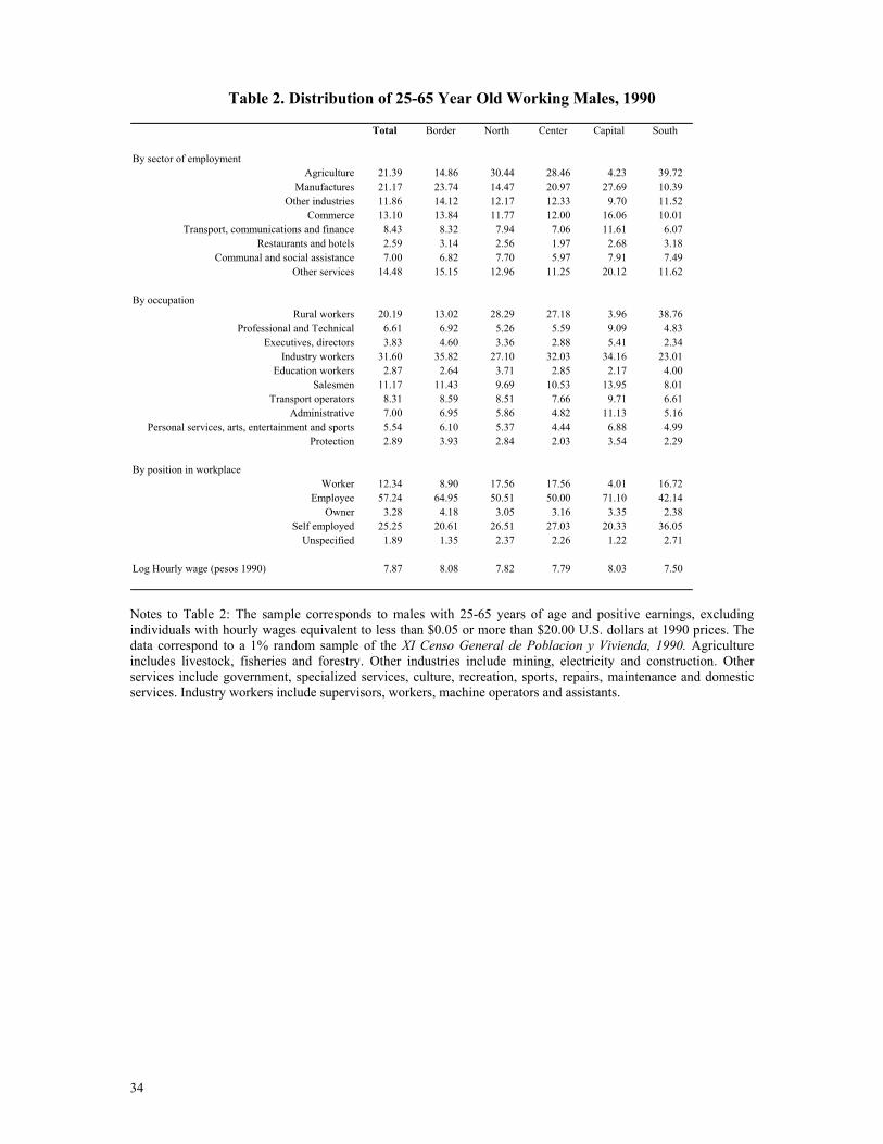
34
Table 2. Distribution of 25-65 Year Old Working Males, 1990
Total Border North Center Capital South
By sector of employmentAgriculture 21.39 14.86 30.44 28.46 4.23 39.72
Manufactures 21.17 23.74 14.47 20.97 27.69 10.39Other industries 11.86 14.12 12.17 12.33 9.70 11.52
Commerce 13.10 13.84 11.77 12.00 16.06 10.01Transport, communications and finance 8.43 8.32 7.94 7.06 11.61 6.07
Restaurants and hotels 2.59 3.14 2.56 1.97 2.68 3.18Communal and social assistance 7.00 6.82 7.70 5.97 7.91 7.49
Other services 14.48 15.15 12.96 11.25 20.12 11.62
By occupation Rural workers 20.19 13.02 28.29 27.18 3.96 38.76
Professional and Technical 6.61 6.92 5.26 5.59 9.09 4.83Executives, directors 3.83 4.60 3.36 2.88 5.41 2.34
Industry workers 31.60 35.82 27.10 32.03 34.16 23.01Education workers 2.87 2.64 3.71 2.85 2.17 4.00
Salesmen 11.17 11.43 9.69 10.53 13.95 8.01Transport operators 8.31 8.59 8.51 7.66 9.71 6.61
Administrative 7.00 6.95 5.86 4.82 11.13 5.16Personal services, arts, entertainment and sports 5.54 6.10 5.37 4.44 6.88 4.99
Protection 2.89 3.93 2.84 2.03 3.54 2.29
By position in workplace Worker 12.34 8.90 17.56 17.56 4.01 16.72
Employee 57.24 64.95 50.51 50.00 71.10 42.14Owner 3.28 4.18 3.05 3.16 3.35 2.38
Self employed 25.25 20.61 26.51 27.03 20.33 36.05Unspecified 1.89 1.35 2.37 2.26 1.22 2.71
Log Hourly wage (pesos 1990) 7.87 8.08 7.82 7.79 8.03 7.50 Notes to Table 2: The sample corresponds to males with 25-65 years of age and positive earnings, excluding individuals with hourly wages equivalent to less than $0.05 or more than $20.00 U.S. dollars at 1990 prices. The data correspond to a 1% random sample of the XI Censo General de Poblacion y Vivienda, 1990. Agriculture includes livestock, fisheries and forestry. Other industries include mining, electricity and construction. Other services include government, specialized services, culture, recreation, sports, repairs, maintenance and domestic services. Industry workers include supervisors, workers, machine operators and assistants.

35
Table 3. Distribution of 25-65 Year Old Working Males, 2000
Total Border North Center Capital South
By sector of employmentAgriculture 13.40 8.60 20.20 18.94 2.84 23.70
Manufactures 20.03 25.81 14.95 20.49 21.65 10.18Other industries 14.28 15.07 15.29 14.91 11.56 16.24
Commerce 15.12 14.43 13.83 14.15 18.42 12.81Transport, communications and finance 9.07 8.47 7.00 7.80 12.49 7.71
Restaurants and hotels 3.52 3.80 3.52 2.85 3.63 4.52Communal and social assistance 6.82 6.28 8.32 6.30 6.72 8.10
Other services 17.76 17.53 16.87 14.56 22.69 16.74
By occupation Rural workers 12.82 7.66 18.52 18.44 2.66 23.56
Professional and Technical 7.95 8.23 6.70 6.38 10.80 6.49Executives, directors 3.00 3.53 2.79 2.20 4.05 2.16
Industry workers 33.88 39.60 31.85 35.11 31.65 27.90Education workers 3.12 2.65 4.19 3.12 2.39 4.57
Salesmen 13.21 12.33 12.01 12.78 16.24 10.27Transport operators 8.55 7.89 7.82 7.86 10.24 8.39
Administrative 7.06 7.19 6.24 5.44 9.75 5.99Personal services, arts, entertainment and sports 6.94 7.22 6.16 5.89 8.21 7.14
Protection 3.47 3.71 3.72 2.77 4.01 3.54
By position in workplace Worker 10.22 6.02 15.38 14.71 3.28 16.08
Employee 61.95 69.42 58.43 56.03 68.93 53.18Owner 3.50 4.43 3.86 3.53 2.99 2.76
Self employed 23.24 19.06 21.06 24.60 24.10 26.30Unspecified 1.09 1.07 1.27 1.14 0.70 1.67
Log Hourly wage (pesos 1990) 7.77 8.06 7.75 7.65 7.87 7.41 Notes to Table 3: The sample corresponds to males with 25-65 years of age and positive earnings, excluding individuals with hourly wages equivalent to less than $0.05 or more than $20.00 U.S. dollars at 1990 prices. The data correspond to a 10% random subsample extracted from the 10% sample of the XII Censo General de Poblacion y Vivienda, 2000. Agriculture includes livestock, fisheries and forestry. Other industries include mining, electricity and construction. Other services include government, specialized services, culture, recreation, sports, repairs, maintenance and domestic services. Industry workers include supervisors, workers, machine operators and assistants.

36
Table 4a. Foreign Direct Investment, Maquiladora Employment and Migration Migration rate
Foreign direct investment (% of regional GDP)
Maquiladora employment (% of manuf. employment) (% of 1960
pop.) 1994 2000 1990 1999 1955-1959 Border 2.43 3.77 45.99 60.07 2.04 North 0.43 0.77 5.26 22.84 3.16 Center 0.43 1.37 1.71 8.92 1.52 Capital 6.00 4.44 0.22 1.68 0.23 South 0.24 0.20 2.88 21.54 0.59 Total 2.75 2.80 14.91 29.41 1.40 Source: Constructed with data from INEGI
Table 4b. Foreign Direct Investment, Maquiladora Employment and Migration Migration
Foreign direct investment (% of total FDI)
Maquiladora employment (% of total maq. Employment) (% of total
migrants) 1994 2000 1990 1999 1955-1959 Border 19.16 32.40 93.64 82.52 23.00 North 1.30 2.16 2.33 5.83 26.91 Center 3.96 12.30 2.93 7.97 40.31 Capital 74.67 52.43 0.51 1.29 3.20 South 0.91 0.71 0.59 2.39 6.58 Total 100.00 100.00 100.00 100.00 100.00 Source: Constructed with data from INEGI

37
Table 5. Domestic Migration Flows: Males 25-65 Years Old (Composition of each region’s current population by region of origin)
Region of residencein 1985 Border North Center Capital South
Border 95.69 1.16 0.27 0.23 0.20North 1.77 96.03 0.30 0.15 0.06
Center 1.38 1.14 96.97 1.35 1.12Capital 0.95 1.17 1.91 97.76 1.10
South 0.22 0.50 0.55 0.52 97.51
Total 100.00 100.00 100.00 100.00 100.00
Region of residencein 1990 Border North Center Capital South
Border 96.70 1.87 0.47 0.47 0.27North 1.41 95.76 0.32 0.22 0.11
Center 1.07 1.27 96.98 1.43 1.33Capital 0.46 0.79 1.81 97.30 1.21
South 0.36 0.30 0.41 0.58 97.08
Total 100.00 100.00 100.00 100.00 100.00
Region of residencein 1995 Border North Center Capital South
Border 95.75 1.18 0.36 0.21 0.18North 1.38 96.79 0.28 0.09 0.14
Center 1.81 0.90 97.10 1.18 1.11Capital 0.64 0.65 1.69 98.14 1.05
South 0.41 0.47 0.57 0.37 97.52
Total 100.00 100.00 100.00 100.00 100.00
Region of residence in 1990
Region of residence in 1995
Region of residence in 2000
Notes to Table 5: The sample is all males 25-65 years old. The data correspond to a 1% random sample of the XI Censo General de Poblacion y Vivienda, 1990, a 0.4% sample from the 1995 Conteo de Poblacion and a 10% random subsample extracted from the 10% sample of the XII Censo General de Poblacion y Vivienda, 2000. Individuals who resided in other country in 1985, 1990 or 1995 were excluded from the sample.

38
1990
2000
Cha
nge
1990
2000
Cha
nge
1990
2000
Cha
nge
1990
2000
Cha
nge
1990
2000
Cha
nge
Con
stan
t6.
106
5.92
2-0
.184
6.12
25.
944
-0.1
776.
875
6.51
9-0
.356
6.27
65.
817
-0.4
596.
626
5.69
5-0
.931
(152
.28)
(154
.40)
(3.3
1)(1
51.8
2)(1
54.0
9)(3
.18)
(161
.15)
(160
.17)
(6.0
4)(8
1.34
)(8
7.02
)(4
.49)
(55.
64)
(71.
85)
(6.5
1)
Age
0.04
90.
035
-0.0
140.
049
0.03
5-0
.013
0.03
30.
023
-0.0
100.
031
0.02
3-0
.008
0.03
20.
023
-0.0
08(2
4.24
)(1
8.04
)(4
.84)
(24.
21)
(18.
10)
(4.7
9)(1
7.06
)(1
2.28
)(3
.83)
(16.
36)
(12.
69)
(3.0
5)(1
6.54
)(1
2.91
)(3
.06)
Age
2 /100
-0.0
49-0
.030
0.01
8-0
.049
-0.0
300.
018
-0.0
33-0
.022
0.01
2-0
.032
-0.0
230.
009
-0.0
32-0
.023
0.01
0(2
0.31
)(1
2.87
)(5
.48)
(20.
32)
(12.
97)
(5.4
3)(1
4.49
)(9
.63)
(3.6
9)(1
4.27
)(1
0.41
)(2
.99)
(14.
38)
(10.
51)
(3.0
3)
Yea
rs o
f sch
oolin
g0.
078
0.10
00.
022
0.07
60.
097
0.02
10.
034
0.05
30.
019
0.02
80.
048
0.01
90.
029
0.04
80.
019
(144
.04)
(185
.20)
(28.
36)
(83.
06)
(108
.18)
(16.
22)
(17.
09)
(27.
64)
(6.8
1)(1
4.38
)(2
5.20
)(6
.99)
(14.
61)
(25.
62)
(7.0
8)
Mar
ried
0.08
50.
078
-0.0
070.
087
0.08
2-0
.005
0.07
00.
083
0.01
30.
082
0.09
60.
014
0.07
90.
095
0.01
6(1
1.28
)(1
1.57
)(1
1.28
)(1
1.64
)(1
2.24
)(0
.50)
(9.6
5)(1
2.88
)(1
.31)
(11.
29)
(15.
04)
(1.4
5)(1
0.97
)(1
5.08
)(1
.70)
Bor
der
0.17
60.
287
0.11
10.
193
0.33
10.
139
0.12
70.
318
0.19
1-0
.118
0.08
50.
203
-0.5
33-0
.502
0.03
0(2
3.71
)(4
0.05
)(1
0.75
)(1
4.48
)(2
1.80
)(6
.87)
(9.8
4)(2
1.62
)(9
.75)
(5.6
0)(4
.30)
(7.0
2)(1
7.14
)(1
5.60
)(0
.68)
Nor
th0.
014
0.05
00.
036
0.06
90.
120
0.05
20.
073
0.14
50.
073
0.00
20.
089
0.08
8-0
.122
-0.0
820.
040
(1.4
4)(5
.56)
(2.7
9)(4
.42)
(7.1
3)(2
.26)
(4.8
2)(9
.24)
(3.3
3)(0
.10)
(5.0
5)(3
.64)
(6.5
1)(4
.26)
(1.5
0)
Cap
ital
0.06
00.
045
-0.0
150.
002
-0.1
08-0
.110
-0.1
11-0
.111
-0.0
01-0
.320
-0.3
44-0
.024
-0.2
82-0
.277
0.00
5(8
.98)
(7.0
8)(1
.68)
(0.1
6)(7
.93)
(6.0
0)(9
.10)
(8.5
4)(0
.03)
(16.
49)
(20.
12)
(0.9
3)(1
0.95
)(1
3.56
)(0
.14)
Sout
h-0
.242
-0.2
180.
024
-0.3
09-0
.277
0.03
2-0
.258
-0.2
65-0
.007
-0.1
76-0
.149
0.02
7-0
.149
-0.0
620.
086
(26.
83)
(26.
61)
(1.9
6)(2
1.78
)(1
8.87
)(1
.56)
(19.
13)
(19.
52)
(0.3
8)(1
0.84
)(9
.89)
(1.2
1)(8
.36)
(3.9
1)(3
.61)
Bor
der*
Scho
olin
g-0
.002
-0.0
04-0
.003
0.00
4-0
.005
-0.0
090.
007
-0.0
02-0
.009
0.00
8-0
.001
-0.0
09(1
.08)
(2.8
4)(1
.30)
(2.8
7)(3
.12)
(4.2
4)(5
.09)
(1.3
3)(4
.51)
(5.6
8)(0
.74)
(4.5
0)
Nor
th*S
choo
ling
-0.0
08-0
.008
0.00
0-0
.006
-0.0
10-0
.004
-0.0
04-0
.008
-0.0
04-0
.005
-0.0
09-0
.004
(4.4
9)(4
.71)
(0.0
7)(3
.40)
(5.7
7)(1
.52)
(2.5
2)(5
.05)
(1.6
8)(2
.84)
(5.0
8)(1
.46)
Cap
ital*
Scho
olin
g0.
007
0.01
60.
009
0.01
40.
014
0.00
00.
016
0.01
50.
000
0.01
70.
015
-0.0
01(5
.38)
(11.
89)
(4.7
6)(1
0.77
)(1
0.82
)(0
.09)
(11.
77)
(11.
42)
(0.2
5)(1
2.45
)(1
1.46
)(0
.70)
Sout
h*Sc
hool
ing
0.01
10.
008
-0.0
040.
009
0.00
7-0
.002
0.00
90.
007
-0.0
020.
010
0.00
7-0
.003
(6.5
6)(4
.59)
(1.5
7)(5
.56)
(4.5
2)(1
.02)
(5.3
5)(4
.71)
(0.7
7)(5
.77)
(4.6
9)(1
.10)
Posi
tion,
occ
upat
ion,
sect
or d
umm
ies
No
No
No
No
Yes
Yes
Yes
Yes
Yes
Yes
Site
-spe
cific
feat
ures
No
No
No
No
No
No
Yes
Yes
Yes
Yes
Glo
baliz
atio
n co
ntro
lsN
oN
oN
oN
oN
oN
oN
oN
oY
esY
es
R2
0.22
20.
347
0.22
30.
349
0.30
70.
434
0.32
40.
451
0.32
90.
458
N99
528
1285
1499
528
1285
1497
086
1263
8597
086
1263
8597
086
1263
85
(e)
(a)
(b)
(c)
(d)
Not
es: C
oeff
icie
nts a
re fo
r OLS
regr
essi
ons u
sing
the
log
aver
age
hour
ly w
age
as d
epen
dent
var
iabl
e, w
here
the
wag
e is
mea
sure
d in
19
90 p
esos
. The
T st
atis
tics i
n pa
rent
hese
s are
bas
ed o
n he
tero
sked
astic
ity-c
onsi
sten
t sta
ndar
d er
rors
. The
sam
ple
corr
espo
nds t
o m
ales
w
ith 2
5-65
yea
rs o
f age
and
pos
itive
ear
ning
s, ex
clud
ing
indi
vidu
als w
ith h
ourly
wag
es e
quiv
alen
t to
less
than
$0.
05 o
r mor
e th
an
$20.
00 U
.S. d
olla
rs a
t 199
0 pr
ices
.
Tab
le 6
. Ind
ivid
ual W
age
Reg
ress
ion
Res
ults

39
Table 7. Regression Results for Changes in Zero-Schooling Wages and Returns to Schooling
(a) (b) (c) (d) (a) (b) (c) (d)
Constant -0.046 -0.417 -1.822 -1.858 0.012 0.030 0.163 0.163(0.61) (3.87) (5.30) (5.63) (2.62) (3.48) (4.60) (4.87)
Rural dummy -0.138 -0.138 -0.138 -0.138 -0.007 -0.007 -0.007 -0.007(4.34) (4.64) (6.20) (6.52) (2.73) (2.76) (2.75) (2.84)
Agriculture share in GDP (1993-2000) 1.061 0.884 -0.063 -0.075 (1.76) (2.54) (1.03) (1.94)
Manufacturing share in GDP (1993-2000) 1.776 1.466 -0.077 -0.086 (4.60) (7.27) (1.88) (4.04)
Large manuf. firms (% of total manuf. firms in 1988) -17.592 -18.301 1.346 1.400 (2.85) (4.63) (2.25) (3.16)
1990 log(Population density) -0.050 -0.050 0.002 0.003(1.94) (2.88) (0.65) (1.29)
1990 non-literacy rate 0.428 0.451 -0.077 -0.075(0.90) (1.22) (1.57) (2.15)
1990 telephone lines per 100 persons -0.049 -0.062 0.005 0.005(3.45) (4.21) (3.16) (3.27)
1990 number of international airports 0.065 0.058 -0.002 -0.002(2.39) (3.00) (0.81) (1.01)
1990 average schooling years in state 0.102 0.109 -0.013 -0.013(2.67) (2.89) (3.42) (3.96)
Log(Distance to US) -0.040 0.009 0.093 0.110 0.001 -0.002 -0.009 -0.008(3.65) (0.60) (3.45) (3.97) (1.00) (1.41) (2.60) (2.45)
Maquiladora employment share (1990-1999) 1.424 1.136 -0.116 -0.123 (1.69) (2.25) (1.55) (2.07)
Foreign direct investment share in GDP (1994-2000) 14.515 16.769 -1.071 -1.088 (4.12) (4.78) (2.37) (2.59)
Historical migration rates (1955-1959) 3.823 4.306 -0.165 -0.171 (3.44) (4.41) (1.44) (1.72)
Border dummy 0.183 -0.108 -0.009 -0.004(2.92) (0.83) (1.95) (0.33)
North dummy 0.096 0.029 -0.004 -0.002(2.20) (0.46) (0.99) (0.34)
Capital dummy -0.040 -0.007 0.006 0.002(0.86) (0.07) (1.24) (0.20)
South dummy -0.043 0.059 0.001 0.001(0.91) (0.88) (0.30) (0.08)
R2 0.325 0.450 0.752 0.740 0.116 0.188 0.430 0.428
F test for Region dummies = 0 --- 3.99 0.49 --- --- 1.66 0.05 ---prob. --- 0.006 0.747 --- --- 0.172 0.994 ---
Chi-squared test for overidentifying restrictions --- --- 5.372 6.593 --- --- 6.156 6.807prob. --- --- 0.251 0.581 --- --- 0.188 0.558
Change in zero schooling wage level Change in returns to schooling
Note. T statistics in parentheses are based on heteroskedasticity-consistent estimates of standard errors. See main text for a description of the procedure used to construct these estimates.

40
Figure 1. Regional Distribution of Manufacturing Employment in Mexico (%) */ ( )
05
101520253035404550
1930 1940 1950 1960 1970 1980 1985 1993 1998
Mexico CityBorder
*/ Data for the border region before 1970 is unavailable Source: Hanson (1998a) and Mexico’s Industrial Censuses, INEGI

41
Figure 2. White Collar/Blue Collar Hourly Wage Ratio in Manufacturing Industry
1.8
2.0
2.2
2.4
2.6
2.8
3.0
3.2
1980 1982 1984 1986 1988 1990 1992 1994 1996 1998 2000 2002
GATT
NAFTA
1.8
2.0
2.2
2.4
2.6
2.8
3.0
3.2
1980 1982 1984 1986 1988 1990 1992 1994 1996 1998 2000 2002
GATT
NAFTA
GATT
NAFTA
Source: Computed with data from INEGI.

42
Figure 3. Mexico’s Regional Breakup
Border
North
Center
Capital
South

43
Figure 4. Two Region Model Under Autarky L
Good i
H
Good a
Good t
(w/q) B
(w/q)R

44
Figure 5. Two Region Model Under Free Trade L
Good i
H
Good a
Good t
(w/q) B
(w/q)R

45
Figure 6. Three Region Model Under Autarky L
H
(w/q) M
(w/q) B
(w/q) S
Good t
Good a
Good i
Good b

46
Figure 7. Three Region Model Under Free Trade L
H
(w/q) M
(w/q) B
(w/q) S
Good t
Good a
Good i
Good b

47
Figure 8. Two Region Model, With Transport Costs
L
Good iH
Good a
Good t (w/q) B
(w/q)R
Border
Border
Rest of country
Rest of country
Border
Rest of country

48
Appendix A.
In this appendix, I show that, in principle, it is possible to correct the standard errors of
the regressions in Table 7 for the fact that the dependent variables are themselves estimated
coefficients. I also show that biases may result in negative estimates for relevant variances.
Formally, let β denote the (64×1) vector of true changes in returns to schooling (or
zero-schooling wages) between 1990 and 2000 and β be the vector of estimated values for
these changes, extracted from the first-step OLS regressions described in the main text. It is
possible to write the relation between these two as εββ S+=ˆ , where ε is a vector of i.i.d.
N(0,1) random variables and Ω=′SS is the variance-covariance matrix for β . Let Ω denote the
estimate of this matrix. Assume the true β is related to site-specific features and state-level
globalization measures according to ηγβ += X . X is a (64×k) matrix of observations for k site-
specific features and globalization measures, γ is an k×1 vector of unknown coefficients and η
denotes the vector of disturbance terms associated with this regression. Assume that ε is
uncorrelated with η. Note that this corresponds to the specification of the second step
regressions described in the main text.
The immediate problem is that β is unobserved, so in the regressions I use β instead.
Combining the expressions above, the estimated regressions correspond to εηγβ SX ++=ˆ . Let
γ denote the OLS estimate of the coefficients in this regression. Given the expression above,
the appropriate variance-covariance matrix of γ is 1'1'12 )'()()'( −−− Ω+ XXXXXXXXησ , where 2ησ is
the variance of η. In order to compute this matrix, we need an estimate for 2ησ . If u denotes the
residual vector from the OLS regression of β on X, uu ′ may be treated as an estimate of
Ω+I2ησ . Thus, an estimate of 2
ησ can be obtained by averaging the diagonal elements of
Ω−′ ˆuu . Given this estimate, the standard errors of γ are computed by plugging into the
expression above the corresponding estimates for 2ησ and Ω. Note, however, that if the
assumption that ε is uncorrelated with η is not satisfied, this procedure does not guarantee a
positive estimate for 2ησ which, in fact, will be biased. This in turn may cause the presence of
negative variances for some elements of γ .

49
References
Airola, Jim (2001). “Trade and Wages: A Regional Analysis of the Effects of Trade on Wages in Mexico”. University of Houston. Unpublished manuscript. Alvarez, Roberto and Raymond Robertson (2001). “Exposure to Foreign Markets and Firm-level Innovation: Evidence From Chile and Mexico.” Macalester College, Department of Economics. Unpublished manuscript. Baldwin, Robert and Glen Cain (1997). “Shifts in U.S. Relative Wages: The Role of Trade, Technology and factor Endowments” NBER Working Paper No. w5934. Berman, Eli, John Bound and Zvi Griliches (1994). “Changes in Demand for Skilled Labor Within US Manufacturing: Evidence from the Annual Survey of Manufactures”. Quarterly Journal of Economics, 109(2): 367-397. Brown, Drusilla, Alan Deardorff and Robert Stern (1992). “North American Integration.” The Economic Journal, 102(415): 1507-1518. Chiquiar, Daniel (2003). “Why Mexico’s regional income convergence broke down”. Banco de México. Unpublished manuscript. Chiquiar, Daniel and Gordon Hanson (2002). “International Migration, Self-Selection and the Distribution of Wages: Evidence from Mexico and the United States”. NBER Working Paper No. w9242. Cornelius, Wayne (2002). “Impacts of NAFTA on Mexico-to-U.S. Migration.” In Chambers, Edward and Peter Smith, NAFTA in the New Millenium, Center of U.S.-Mexican Studies, University of California, San Diego and The University of Alberta Press: 287-304. Cragg, Michael and Mario Epelbaum (1996). “Why Has Wage Dispersion Grown in Mexico? Is it the Incidence of Reforms or the Growing Demand for Skills?” Journal of Development Economics, 51(1): 99-116. Dávila, Enrique, Georgina Kessel and Santiago Levy (2002). “El Sur También Existe: Un Ensayo Sobre el Desarrollo Regional de México”. Unpublished manuscript. Davis, Donald (1996). “Trade Liberalization and Income Distribution” NBER Working Paper No. w5693. Durand, Jorge, William Kandel, Emilio Parrado and Douglas S. Massey. 1996. “International Migration and Development in Mexican Communities.” Demography 33(2): 249-264. Esquivel, Gerardo (1999). “Convergencia Regional en México, 1940-1995.” El Trimestre Económico, 66(4): 725-761.
Esquivel, Gerardo and Miguel Messmacher (2002). “Sources of Regional (non) Convergence in Mexico.” Paper presented at the Wider/Cornell/LSE Mexico Conference on Spatial

50
Inequality in Latin America. Institute of Public Policy and Development Studies, Universidad de las Américas, Puebla. Feenstra, Robert (1998). “Integration of trade and Disintegration of Production in the Global Economy”. Journal of Economic Perspectives, 12(4): 31-50. Feenstra, Robert and Gordon Hanson (1996). “Foreign Investment, Outsourcing and Relative Wages.” In R. Feenstra, G. Grossman and D. Irwin (eds.), Political Economy of Trade Policy: Essays in Honor of Jagdish Bhagwati, MIT Press: 89-127. ---------------- (1997). “Foreign Direct Investment and Relative Wages: Evidence From Mexico’s Maquiladoras.” Journal of International Economics, 42(3-4): 371-393. Freeman, Richard (1995). “Are Your Wages Set in Beijing?”. The Journal of Economic perspectives, 9(3): 15-32. García Verdú, Rodrigo (2002). “Income Dynamics Across States in Mexico: 1940-2000.” Banco de México. Unpublished manuscript. Hanson, Gordon (1996). “Localization Economies, Vertical Organization, and Trade.” American Economic Review, 86(5): 1266-1278. ---------------- (1997). “Increasing Returns, Trade and the Regional Structure of Wages.” The Economic Journal, 107(440): 113-133. ---------------- (1998a). “North American Economic Integration and Industry Location.” Oxford Review of Economic Policy, 14(2): 30-44. ---------------- (1998b). “Regional Adjustment to Trade Liberalization.” Regional Science and Urban Economics, 28(4): 419-444. ---------------- (2003). “What Has Happened to Wages in Mexico Since NAFTA?”. NBER Working Paper No. w9563. Hanson, Gordon and Ann Harrison (1999). “Trade Liberalization and Wage Inequality in Mexico.” Industrial and Labor Relations Review, 52(2): 271-288. Hanson, Gordon and Christopher Woodruff (2002). “Emigration and Educational Attainment in Mexico.” UC San Diego. Unpublished manuscript. Juan Ramón, Hugo and Luis Rivera Bátiz (1996). “Regional Growth in Mexico: 1970-1993.” IMF Working Paper, 96/92. Katz, Isaac (1998). La Apertura Comercial y su Impacto Regional Sobre la Economía Mexicana. ITAM. Krugman, Paul (1995). “Technology, Trade and factor Prices”. NBER Working Paper No. w5355.

51
Krugman, Paul and Raul Livas Elizondo (1996). “Trade Policy and the Third World Metropolis.” Journal of Development Economics, 49(1): 137-150. Lawrence, Robert and Matthew Slaughter (1993). “Trade and U.S. Wages: Giant Sucking Sound or Small Hiccup?”. Brookings Papers of Economic Activity, Microeconomics. Brookings Institution: 161-226. Leamer, Edward (1993). “Wage Effects of a U.S.-Mexican Free Trade Agreement”. In Peter Garber (ed.) The Mexico-U.S. Free Trade Agreement, Cambridge, MIT Press: 57-125. ---------------- (1994). “Trade, Wages and Revolving-Door Ideas”. NBER Working Paper No. w4716. Levy, Santiago and Sweder Van Wijnbergen (1995). “Transition Problems in Economic Reform: Agriculture in the North American Free Trade Agreement.” American Economic Review, 85(4): 738-754. López-Córdova, Ernesto (2001). “NAFTA and the Mexican Economy: Analytical Issues and Lessons for the FTAA.” Inter-American Development Bank. INTAL-ITD-STA Occasional Paper 9. Lustig, Nora (2001). “Life is not Easy: Mexico’s Quest for Stability and Growth.” Journal of Economic Perspectives, 15(1): 85-106. Markusen, James and Stephen Zahniser (1997). “Liberalization and Incentives for Labor Migration: Theory With Applications to NAFTA.” NBER Working Paper 6232. Martin, Philip (1993). Trade and Migration: NAFTA and Mexican Agriculture. Institute of International Economics, Washington. Massey, Douglas and Kristin Espinoza (1997). “What’s Driving Mexico-U.S. Migration? A Theoretical, Empirical and Policy Analysis.” American Journal of Sociology, 102(4): 939-999. Meardon, Stephen (2003). “Geography, Trade and Regional Disparities: The Case of the Missing Middle of Mexico”. Inter-American Development Bank. Unpublished manuscript. Melendez, Jorge (2001). “The Structure of Wages Under Trade Liberalization: Mexico from 1984 to 1998”. PhD. Dissertation, University of Chicago. Messmacher, Miguel (2000). “Desigualdad Regional en México. El Efecto del TLCAN y Otras Reformas Estructurales.” Research Document 2000-4, Banco de México. Mishra, Prachi (2003). “Emigration and Wages in Source Countries: Evidence from Mexico.” Columbia University. Unpublished manuscript. Revenga, Ana (1997). “Employment and Wage Effects of Trade Liberalization: The Case of Mexican Manufacturing.” Journal of Labor Economics, 15(3): 520-543. Revenga, Ana and Claudio Montenegro (1998). “North American Integration and Factor Price Equalization: Is There Evidence of Wage Convergence Between Mexico and the United

52
States?.” In Collins, Susan (ed.), Imports, Exports and the American Worker. The Brookings Institution: 305-347. Richardson, J. David (1995). “Income Inequality and Trade: How to Think, What to Conclude”. The Journal of Economic perspectives, 9(3): 33-55. Robertson, Raymond (2000a). “Trade Liberalization and Wage Inequality: Lessons from the Mexican Experience.” World Economy 23(6): 827-849. ---------------- (2000b). “Exposure to Foreign Markets, Production Technology and the Demand for Skill: Evidence From Mexico.” Macalester College, Department of Economics. Unpublished manuscript. ---------------- (2001). “Relative Prices and Wage Inequality: Evidence From Mexico.” Macalester College, Department of Economics. Unpublished manuscript. Rodríguez-Pose, Andrés and Javier Sánchez-Reaza (2002). “Economic Polarization through Trade: the Impact of Trade Liberalization on Mexico’s Regional Growth.” Paper presented at the Cornell/LSE/Wider Conference on Spatial Inequality and Development. London School of Economics. Sachs, Jeffrey and Howard Shatz (1996). “U.S. Trade with Developing Countries and Wage Inequality”. American Economic Review, 86(2): 234-239. Taylor, Edward (1992). “Remittances and Inequality Reconsidered: Direct, Indirect and Intertemporal Effects.” Journal of Policy Modeling, 14(2): 187-208. Taylor, Edward, Joaquin Arango, Graeme Hugo, Ali Kouaouci, Douglas Massey and Adela Pellegrino (1996). “Current Items.” Population Index, 62(2): 181-212. Veeman, Michele, Terrence Veeman and Ryan Hoskins (2002). “NAFTA and Agriculture: Challenges for Trade and Policy.” In Chambers, Edward and Peter Smith, NAFTA in the New Millenium, Center of U.S.-Mexican Studies, University of California, San Diego and The University of Alberta Press: 305-329. Venables, Anthony and Nuno Limão (2002). “Geographical Disadvantage: a Heckscher-Ohlin-von Thünen Model of International Specialization.” Journal of International Economics, 58(2): 239-263. Wood, Adrian (1994). North-South Trade, Employment and Inequality: Changing Fortunes in a Skill-Driven World. Oxford, Clarendon Press. ---------------- (1995). “How Trade Hurt Unskilled Workers”. Journal of Economic Perspectives, 9(3): 57-80. Woodruff, Christopher and Rene M. Zenteno (2002). “Remittances and Microenterprises in Mexico.” UC San Diego. Unpublished manuscript.