Globally Optimal Design Optimization of Cooling Water Systems

Globally Optimal Design Optimization of Cooling Water SystemsAna L. L. Levy,† Jaime N. M. Souza,‡ Miguel J. Bagajewicz,§ and Andre L. H. Costa*,†

†Institute of Chemistry, Rio de Janeiro State University (UERJ), Rua Sao Francisco Xavier, 524, Maracana, Rio de Janeiro, RJ, CEP20550-900, Brazil‡LEPABE, Department of Chemical Engineering, Faculty of Engineering, University of Porto, Rua Dr. Roberto Frias, s/n, 4200-465Porto, Portugal§School of Chemical, Biological and Materials Engineering, University of Oklahoma, Norman, Oklahoma 73019, United States

*S Supporting Information

ABSTRACT: This study presents a globally optimal linearprocedure for the simultaneous design of cooling watersystems. The optimization entails obtaining optimal pipediameters, pump selection, and detailed cooler design. For thelatter, the Kern model and the linear formulation proposed byGoncalves et al. (Ind. Eng. Chem. Res. 2017, 56, 5970) wereused. The proposed linear model is compared with conven-tional design procedures, such as optimizing the design ofeach exchanger first, through area minimization or througharea and pressure drop costs. The results illustrate in one ofthe examples the advantage of using the proposedsimultaneous design approach.

1. INTRODUCTION

Typical cooling water systems are composed of a cooling towerconnected to a pipe network and one or more pumps, whichdistribute cooling water to a set of coolers, which, in mostcases, are aligned in parallel. There are three components tothis problem: the cooling water heat exchanger network vis-a-vis its use and reuse structure with a priori known coolingtasks; the associated hydraulic issues; and the design of thecooling water tower. Studies about these structures related totheir optimal design and operation started in only the early2000s.For the case of the cooling heat exchanger network, Kim and

Smith1,2 proposed the use of the pinch design method todetermine what is the appropriate reuse of cooling water. Kimet al.3 augmented this modeling by analyzing the interactionswith the cooling tower. The problem was put in a form of amathematical model using a water main by Feng et al.4 Picon-Nunez et al.5 studied the effect of the network arrangement onthe total area of the exchangers upon reuse of cooling water.Later, Ponce-Ortega et al.6 presented a mixed-integer nonlinearprogramming (MINLP) formulation based on the Synheatmodel7 of cooling water to synthesize the network, thusallowing the reuse of water.A limited number of follow-up papers addressed the

hydraulic analysis of the pipe network associated with coolingwater systems. Picon-Nunez et al.8 investigated the issue byproposing a simplified hydraulic model of the pipe networkand the set of coolers. Picon-Nunez et al.9 investigated theimpact of the insertion of new heat exchangers in a coolingwater system, including the analysis of the behavior of the

cooling tower heat load and aspects related to fouling. Sun etal.10 employed simulated annealing for the design optimizationof an auxiliary pumping system associated with cooling waternetworks, although pipe diameters were not optimized. DeSouza et al.11 proposed the hydraulic design of cooling waterdistribution systems based on the solution of a set of linearprogramming problems. The solution determines the pumpsize and diameters of the pipe sections (represented by thelengths of the subsections of commercial diameters). Finally,Souza et al.12 investigated the optimization of the hydraulicdebottlenecking of cooling water systems, by means ofsubstituting pipes and pumps together with the manipulationof valves to redistribute the total flow rate among the differentcoolers.Another aspect of the investigation of cooling water systems

involves the exploration of the simultaneous analysis of thecoolers and the associated piping and pumps. This approachhas received some attention in recent years; however, often thefocus is directed to the heat exchanger network synthesis, andthe details of the design of each cooler are usually ignored (thearea evaluation is based on fixed values of film coefficients)and/or the hydraulic design of the pipe network is onlypartially included in these formulations. Ponce-Ortega etal.13,14 analyzed the coolers in the system including theequipment design optimization (i.e., the film coefficients are

Received: December 30, 2018Revised: March 27, 2019Accepted: May 2, 2019Published: May 2, 2019

Article

pubs.acs.org/IECRCite This: Ind. Eng. Chem. Res. 2019, 58, 9473−9485

© 2019 American Chemical Society 9473 DOI: 10.1021/acs.iecr.8b06478Ind. Eng. Chem. Res. 2019, 58, 9473−9485

Dow

nloa

ded

via

UN

IV O

F O

KL

AH

OM

A o

n O

ctob

er 1

4, 2

019

at 0

0:37

:00

(UT

C).

See

http

s://p

ubs.

acs.

org/

shar

ingg

uide

lines

for

opt

ions

on

how

to le

gitim

atel

y sh

are

publ

ishe

d ar

ticle

s.

pubs.acs.org/IECR

http://pubs.acs.org/action/showCitFormats?doi=10.1021/acs.iecr.8b06478

http://dx.doi.org/10.1021/acs.iecr.8b06478

resultant from the heat exchanger design alternatives selected),but the hydraulic design of the pipe network was not fullyexplored in these formulations; that is, the dimensioning ofpipe diameters and the associated pressure drop were notconsidered in the model. Sun et al.15 developed a stepwiseoptimization method for a cooling water system: the first stepuses a model to obtain the optimal cooler network based onparallel branches with several coolers in each branch, and thesecond step employs a simplified hydraulic model to obtain theoptimal pump network with auxiliary pumps installed inparallel branch pipes but with fixed pipe diameters and lengths.Ma et al.16 also investigated the arrangement of the coolers andthe hydraulic aspects, indicating the importance of thesimultaneous optimization of the cooler network and thepump network. They also conducted their analysis ignoring thepiping pressure drop and allowing the same configuration ofseveral branches where several coolers in series can beinstalled. Liu et al.17 investigated the simultaneous synthesisof the heat exchanger network associated with the processstreams and the cooling water system. The model considers thepressure drop in the heat exchangers but also ignores the pipesections, including in the objective function the capital andoperating costs associated with the pumps. Note that Polley etal.18 pointed out that piping may have a considerable impacton the total costs of heat-transfer systems.In relation to the numerical aspects, the majority of the

resultant mathematical formulations in the literature isnonconvex MINLP problems whose solutions, when con-verged, may be trapped in local optima.Hitherto, despite the importance of the simultaneous

analysis of the hydraulic design and the heat exchanger designin cooling water systems, the design practice has been to solvethe problems separately. Each cooler is designed assuming amaximum pressure drop associated with the streams flow, andthe design of the pipe network for the selection of the pumpand pipe section diameters is conducted using a fixed pressuredrop for the coolers. Thus, this practice yields nonoptimalsolutions because they do not explore the interrelationbetween the capital costs of coolers, pipe sections, andpumps and the operating costs of the pumps.In this article, the piping network, the pump, and the

detailed design of the exchangers are considered simulta-neously. First, the overall model is discussed, followed by thenetwork model specifics and the heat exchanger linear model.Then, results are presented, where the advantage of theproposed approach in relation to the conventional approach isdemonstrated. Finally, the conclusions are presented.

2. COOLING SYSTEM MODEL

An optimization solution for the simultaneous design of thecoolers and the pipe network of cooling water systems, not

including the cooling tower, is presented. The objectivefunction is the minimization of the total annualized cost, andthe constraints refer to pipe network modeling, heat exchangermodeling, and economic equations. The problem solutionprovides the optimal set of the design variables of each cooler,the diameter of each pipe section, the head losses in the valves,and the pump size to be selected.Although the literature explores parallel−series arrange-

ments introduced by the pioneering work of Kim and Smith1

and expanded by several papers afterward, the parallel layoutwithout reuse is still the most common alternative found inpractice. This parallel architecture was considered for tworeasons:

• The reuse of water implies that a higher temperature ofthe water is used in downstream units, which promptshigher fouling rates. Until the impact of fouling, the costof elevating the quality of the water, removingsubstances that contribute to the fouling, or the costof frequent cleaning is considered, it is prudent to stayaway from reuse.

• Most important, the reuse is only reasonably covered byall the published models that use water-pinch type ofdesign procedures or stages superstructures,7 when allthe coolers are in the same plant in a complex. When thesystem encompasses serving cooling water to severalcoolers in different plants, reuse involves piping goingfrom one plant to another or possibly back and forth ifthe cost of piping is not considered. As a consequence,all the models considering reuse without adding the costof connections are impractical.

Instead of using continuous variables to describe pipediameters and pump sizing, the proposed formulation usesdiscrete commercial alternatives (e.g., the pipe diameters areselected according to a pipe schedule table and the pumpsizing is coherent with a set of available pump curves).Therefore, the mathematical optimization problem can beformulated as an integer linear programming (ILP), and itssolution is the global optimum. Thus, in contrast with localMINLP approaches, the possibility of being trapped in a poorlocal optimum is excluded and the need of good initialestimates to promote convergence is eliminated.

3. PIPING NETWORK MODELThe proposed analysis of the cooling water system assumesthat the flow rates of the water and process streams in thecoolers and the pipe section lengths are previously fixed; thatis, the mass and energy balances and the layout of the system isthe starting point of the optimization problem. The problemdesign variables are the pipe diameters of the pipe sections, thepump selection, the head losses of the valves associated witheach heat exchanger to guarantee the hydraulic balance

Figure 1. Cooling water system representation.

Industrial & Engineering Chemistry Research Article

DOI: 10.1021/acs.iecr.8b06478Ind. Eng. Chem. Res. 2019, 58, 9473−9485

9474


according to the design flow rate, and the heat exchangergeometry (tube length, tube diameter, tube layout, tube pitchratio, number of baffles, shell diameter, and number of tubepasses).The elements that compose the system are represented

using graph theory.19 The edges (k ∈ STR) represent the heatexchangers (HE ⊂ STR), pipe sections (PI ⊂ STR), and pumps(PU ⊂ STR). The nodes (t ∈VET) represent the cooling towerbasin (PS ⊂ VET), the cooling tower top (PD ⊂ VET), and theinterconnections among the edges (INT ⊂ VET). The coolingtower basin node represents the cooling water supply to thenetwork, and the cooling tower top represents the coolingwater return to the tower. Figure 1 contains an illustration of atypical cooling water system with its interconnected elements.The network edges are organized according to a set of

independent hydraulic circuits (l ∈ HY). A hydraulic circuit isa path along the digraph starting at the cooling water supplynode and ending at the cooling water return. All edges belongto at least one hydraulic circuit. Each heat exchanger isassociated with a unique circuit. It is assumed that eachhydraulic circuit can be associated with a valve/restrictionplate. The network circuits are described by the matrix l k,Λ ,such that, if l k,Λ = 1, then the edge k belongs to the circuit l,

otherwise, l k,Λ = 0. For example, Table 1 contains therepresentation of the hydraulic circuits of the cooling watersystem depicted in Figure 1.

Because the layout of the system and the necessaryvolumetric flow rate in each cooler are already established(qhel), the flow rates along each network element (qk ) can becalculated, prior to the optimization:

q qhe k STRkl HY

l l k,∑ = Λ ∈∈ (1)

The diameters of the pipe sections must be chosenaccording to a set of available commercial options (n ∈ SD).The values of the standard inner and nominal diameters are

represented by Dnint and Dn

nom (the nominal diameter isidentified in inches, according to the industrial practice),respectively. In turn, pump selection is based on a set ofavailable commercial options (s ∈ SPU). Each available pumpoption s is represented by the corresponding head at the designflow rate. In the presentation of the model, the problemparameters, which are fixed prior to the optimization, arerepresented with the symbol “^” on top.The hydraulic behavior of the pipe network is represented

by a mechanical energy balance along each hydraulic circuit(the kinetic head at the cooling water return is dismissed herebecause of its relatively small value):

fpu z fhe

L fpi fv l HY0

k PUl k k

l HYl k l

k PIl k k k l

, ,

,

∑ ∑

∑

Λ − Δ − Λ

− Λ − = ∈∈ ∈

∈ (2)

where fpuk is the head of the pump k, zΔ the elevationdifference between the top and the bottom of the coolingtower, fhel the head loss along the heat exchanger present inthe hydraulic circuit l, Lk

the pipe section length, fpik theunitary head loss along the pipe section k, and f vl the head lossin the valve/restriction plate associated with the circuit l.Meanwhile, the head loss in the heat exchangers is calculatedas follows:

fhePt yT Ps yT

gl HYl

l c l l h l

w

, ,

ρ=

Δ + Δ

∈

(3)

where wρ is the cooling water density and g is the gravityacceleration; PtlΔ and PslΔ are the pressure drops in the heat

exchanger tube-side and shell-side, respectively, and yT c l, and

yTh l, are parameters that indicate if the cooling water is in the

tube-side (yT 1)c l, = or if the hot process stream is in the

tube-side (yT 1h l, = ). Next, the head loss of pipe section k is

calculated using the Hazen−Williams equation:

fc

q

Dk PI

10.67k

k

k1.85

1.852

4.8704=

∈

(4)

where f k is the unitary head loss, Dk the inner diameter, and c the Hazen−Williams constant. In turn, pipe diameter is adiscrete variable, according to the commercially availablevalues. Therefore, it can be represented by binary variables:

D D y k PIkn SD

nint

k npi,∑= ∈

∈ (5)

where yk npi, is a binary variable that it is equal to 1 if the pipe

section k is composed of a commercial diameter n; otherwise,it is equal to 0. Because the problem solution must present aunique diameter for each pipe section

y k PI1n SD

k npi,∑ = ∈

∈ (6)

The substitution of eq 5 into eq 4 of unitary head loss yieldsa linear constraint:

f pf y k PIkn SD

k n k npi

, ,∑= ∈∈ (7)

where

pfq

c Dk PI n SD10.67

( ),k n

k

nint,

1.852

1.85 4.8704=

∈ ∈

(8)

The head of a pump k is also represented by a linearrelation:

fpu pfpu y k PUks SPU

k s k spu

, ,∑= ∈∈ (9)

where pfpuk s, is the head of the pump model s at the design

flow rate of the edge k. yk spu, is a binary variable that it is equal to

Table 1. Hydraulic Circuits of the Cooling Water SystemPresent in Figure 1

circuit edges

1 pi17, pi1, pi2, he1, pi6, pi162 pi17, pi1, pi3, pi4, he2, pi5, pi15, pi163 pi17, pi1, pi3, pi7, pi9, he3, pi10, pi14, pi15, pi164 pi17, pi1, pi3, pi7, pi8, pi9, he4, pi12, pi13, pi14, pi15, pi16



9475


1,if the pump k corresponds to the available option s;otherwise, it is equal to 0.Because only one pump option must be chosen

y k PU1s SPU

k spu,∑ = ∈

∈ (10)

In order to avoid erosion and fouling, maximum andminimum flow velocity bounds are imposed:

vmaxq

Dk PI

40k

k2π

−

≥ ∈(11)

vminq

Dk PI

40k

k2π

−

≤ ∈(12)

whereq

D

4 k

k2π

is the velocity. Substitution of eq 5 into eqs 11 and

12 yields the following linear relations:

vq

Dy k PImax

4

( )0

n SD

k

nint k n

pi2 ,∑

π−

≥ ∈∈ (13)

vminq

Dy k PI

4

( )0

n SD

k

nint k n

pi2 ,∑

π−

≤ ∈∈ (14)

According to engineering practice, the pipe diameter at thepump suction must be equal or higher than the diameter at thepump discharge:

y D y Dn SD

kps npi

nint

n SDkpd npi

nint

, ,∑ ∑ ≥ ∈ ∈ (15)

where kps and kpd are indices associated with the pumpsuction and discharge, respectively.

4. COOLER DETAILED MODELThe heat exchanger model is based on Goncalves et al.,20

where the design problem of E-type shell-and-tube heatexchangers without phase change is formulated as an integerlinear programming (ILP). The allocation of the process andcooling water streams in the tube-side or in the shell-side isconsidered a designer decision established prior to theoptimization. The design variables are the tube inner andouter diameters (dti and dte), tube length (L), tube layout(lay), tube pitch ratio (rp), number of passes in the tube-side(Ntp), shell diameter (Ds), and number of baffles (Nb).The presentation of the constraints related to the heat

exchanger model is organized here in two parts. First, theoriginal nonlinear thermofluid dynamic model and designequations are presented. For the sake of simplicity, only themain equations of the original nonlinear model are presentedhere ; further details can be found in Goncalves et al.20 Afterthis, a reformulation is implemented to obtain a linear model.The LMTD method is used and, considering a design

margin, “excess area” (Aexc ), the heat-transfer rate equation isrepresented by the following relation:

UAAexc Q

TlmF1

100≥ +

Δ

ikjjjj

y{zzzz

(16)

where U is the overall heat-transfer coefficient, A the heat-transfer area, Q the heat load, TlmΔ the logarithmic meantemperature difference, and F the LMTD correction factor. Inturn, the heat-transfer area is given by

A Ntt dte Lπ= (17)

where Ntt is the total number of tubes (simplified expressionsto represent the relation between the total number of tubesand the design variables can be found in Kakac and Liu21).Finally, the overall heat-transfer coefficient is given by

( )U

Rfs

1

dtedti ht

Rftdtedti

dte

ktube hs

ln

21

dtedti

=+ + + +

(18)

where ktube is the thermal conductivity of the tube wall; Rft

and Rfs are the tube-side and shell-side fouling factors, and htand hs are the convective heat-transfer coefficients of the tube-side and shell-side, respectively. The tube-side and shell-sideheat-transfer coefficients are calculated using the Dittus−Boelter correlation for the tube-side22 and the Kern model forthe shell-side.23

Bounds on pressure drops are represented by

Ps PsdispΔ ≤ Δ (19)

Pt PtdispΔ ≤ Δ (20)

where ΔPs and ΔPt are the pressure drops on the shell-sideand tube-side, and PsdispΔ and PtdispΔ are the correspondingadmissible values, respectively. The pressure drop in the tube-side is calculated using the Darcy−Weisbach equation24 andthe Kern model for the shell-side.23

Additional bounds are applied to velocities and Reynoldsnumbers:

vs vsmin≥ (21)

vs vsmax≤ (22)

vt vtmin≥ (23)

vt vtmax≤ (24)

Res 2 103≥ × (25)

Ret 104≥ (26)

Design standards impose the following geometric bounds:25

lbc Ds0.2≥ (27)

lbc Ds1.0≤ (28)

L Ds3≥ (29)

L Ds15≤ (30)

Design variables have a discrete nature, according to theirphysical nature and/or standard commercially availableoptions. Instead of using separate sets of binaries for eachvariable, a single set of binaries was used. Each individualbinary variable (yrowsrow) identifies a heat exchanger candidate,which represents a combination of values of the designvariables (identified by the multi-index srow). Previous resultsindicate that this approach provides considerable reduction ofthe computational effort.20

The final structure of the set of linear constraints as inGoncalves et al.20 is represented below, adding an extra indexfor each individual heat exchanger (l ∈ HY).Because only one option of heat exchanger must be selected



9476


yrow l HY1srow

srow l,∑ = ∈(31)

After substitution of discrete representation and reformula-tion, the heat-transfer rate equation (eq 16), becomes

( )

QPdte

Pht Pdtiyrow Rft

PdtePdti

yrow

Pdte yrow

ktubeRfs

yrow

Phs

AexcPNtt Pdte PL yrow Tlm F

l HY

ln

2

100100

lsrow

srow

srow l srowsrow l l

srow

srow

srowsrow l

srow

srowPdtePdti srow

ll

srow

srow l

srow l

srowsrow srow srow srow l l srow l

,, ,

,

,

, ,

srow

srow

∑ ∑

∑ ∑

∑π

+

+ + +

≤+

Δ

∈

i

k

jjjjjjjjjjjjjy

{

zzzzzzzzzzzzz

ikjjj

y{zzzi

kjjjjjj

y

{zzzzzz

(32)

where Pdtesrow , Pdtisrow

, and PLsrow are values of the outer and

inner tube diameters and tube length and PNttsrow is the total

number of tubes calculated prior to the optimization for eachsolution alternative. The other parameters in eq 32 areexpressed by

( )Pht

kt Prt

Pdti

PNpt

PNtt

0.023srow l

lmt

t ln

srow

srow

srow,

40.8

1.8

0.8l

l=

πμ

i

kjjjjjj

y

{zzzzzz

(33)

( )Phs

ks Prs

PDeq

PNb

PDs PFAR PL

0.36

( 1)

srow l

lms

s

srow

srow

srow srow srow

,

0.551/3

0.45

0.55

l

l=

+

μ

i

k

jjjjjjjy

{

zzzzzzz (34)

PFARPrp

11

srowsrow

= −

(35)

pDeqaDeq Prp Pdte

PdtePdtesrow

srow srow srow

srowsrow

2 2

π= −

(36)

aDeqPlay

Play

4 if 1

3.46 if 2srow

srow

srow

==

=

lmoooo

noooo (37)

( )F

R

RPNpt

PNpt

( 1) ln

( 1)lnif 1

1 if 1

srow l

lP

R P

lP R R

P R R

srow

srow

,

2 0.5 (1 )(1 )

2 ( 1 ( 1) )

2 ( 1 ( 1) )

l

l l

l l l

l l l

2 0.5

2 0.5=

+

−≠

=

−

−

− + − +

− + + +

l

m

oooooooooo

n

oooooooooo

ikjjj

y{zzz

(38)

where mtl and msl are the mass flow rates in the tube-side and

shell-side, respectively; ktl and ktl

are the thermal conductiv-ities; tlμ and slμ are the viscosities; Prtl and Prsl are the Prandtl

Numbers; PNpt srow is the value of the number of tube passes;

PNbsrow is the value of the number of baffles; Prpsrow

is the value

of the tube pitch ratio; Playsrow is the indication of the tube

layout arrangement; and Rl and Pl

are parameters for theevaluation of the correction factor of the LMTD.22

The constraints related to bounds on pressure drops,velocities, Reynolds numbers, and geometrical are representedin an alternative way, where the violation of these constraintsfor each solution candidate can be identified prior to theoptimization, and for these options, an exclusion constraint isadded, as presented below. According to Souza et al.,26 thisprocedure allows a better computational performance.Pressure drop bounds (equivalent to eqs 19 and 20):

yrow srow SDPsmaxout l HY0 for andsrow l, = ∈ ∈(39)

yrow srow SDPtmaxout l HY0 for andsrow l, = ∈ ∈(40)

The sets SDPsmaxoutl and SDPtmaxoutl are given by (whereε is a small positive number)

SDPsmaxout srow P Ps Psdisp/l srow l, ε= { Δ ≥ Δ + } (41)

SDPtmaxout srow P Ptturb P Ptturb

P Ptcab K Ptdisp

/ 1 2l srow l srow l

srow l srow

, ,

, ε

= { Δ + Δ

+ Δ ≥ Δ − }

(42)

where

P Psms s

s

PNb

PDs PFAR PL PDeq

0.864

( 1)

( )

srow ll

srow

srow srow srow srow

,

1.812 0.188

2.812

0.812 1.812 1.188

μρ

Δ =

+

i

k

jjjjjjjy

{

zzzzzzz(43)

P Ptturbmtt

PNpt PL

PNtt Pdti1

0.112srow l

l

l

srow srow

srow srow,

2

2

3

2 5π ρΔ =

i

kjjjjjj

y

{zzzzzzi

k

jjjjjjjy

{

zzzzzzz(44)

P Ptturbmt t

t

PNpt PL

PNtt Pdti2 0.528

4srow l

l l

l

srow srow

srow srow,

1.58 1.58 0.42

1.58

2.58

1.58 4.58

μπ ρ

Δ =

i

k

jjjjjjjy

{

zzzzzzz(45)

P Ptcabmt

t

PNpt

PNtt Pdti

8srow l

l

l

srow

srow srow,

2

2

3

2 4π ρΔ =

i

kjjjjjj

y

{zzzzzz (46)

It is important to note that eqs 39 and 40 are not included inthe formulation for the cooling water streams. In this case, theoptimal pressure drop will be obtained through the trade-offbetween capital and operating costs in the context of the entiresystem solution.Flow velocity bounds (equivalent to eqs 21−24):

yrow srow Svsminout Svsmaxout l HY0 for ( ) andsrow l, = ∈ ∪ ∈(47)

yrow srow Svtminout Svtmaxout l HY0 for ( ) andsrow l, = ∈ ∪ ∈(48)

where the sets Svsminout, Svsmaxout, Svtminout, and Svtmaxoutare given by



9477


Svsminout srowms

s

PNb

PDs PFAR PL

vsmin

/( 1)

ll srow

srow srow srowρ

ε

=+

≤ −

lmooonooo

|}ooo~ooo (49)

Svsmaxout srowms

s

PNb

PDs PFAR PL

vsmax

/( 1)

ll srow

srow srow srowρ

ε

=+

≥ +

lmooonooo

|}ooo~ooo (50)

Svtminout srowmt

t

PNpt

PNtt Pdtivtmin/

4l

l srow

srow srow2πρ

ε= ≤ −

lmooonooo

|}ooo~ooo(51)

Svtmaxout srowmt

t

PNpt

PNtt Pdtivtmax/

4l

l srow

srow srow2πρ

ε= ≥ +

lmooonooo

|}ooo~ooo

(52)

Reynolds number bounds (equivalent to eqs 25 and 26):

yrow srow Resminout l HY0 for andsrow l, = ∈ ∈ (53)

yrow srow Retminout l HY0 for andsrow l, = ∈ ∈ (54)

where the sets Resminout and Retminout are given by

Resminout srowms

s

PDeq PNb

PDs PFAR PL/

( 1)

2 10

l srow srow

srow srow srow

3

μ

ε

=+

≤ × −

lmooonooo

|}ooo~ooo (55)

Retminout srowmt

t

PNpt

PNtt Pdti/

410l srow

srow srow

4

πμε= ≤ −

lmooonooo

|}ooo~ooo

(56)

Baffle spacing bounds (equivalent to eqs 27 and 28):

yrow srow SLNbminout S bmaxout0 for ( ln )srow l, = ∈ ∪(57)

where the sets SLNbminout and SLNbmaxout are given by

SLNbminout srowPL

PNbPDs/

10.2srow

srowsrow ε=

+≤ −

lmoonoo

|}oo~oo(58)

SLNbmaxout srowPL

PNbPDs/

11.0srow

srowsrow ε=

+≥ +

lmoonoo

|}oo~oo(59)

Tube length/shell diameter ratio bounds (equivalent to eqs29 and 30):

yrow srow SLDminout SLDmaxout0 for ( )srow l, = ∈ ∪(60)

where the sets SLDminoutl and SLDmaxoutl are given by

SLDminout srow PL PDs/ 3srow srow ε= { ≤ − } (61)

SLDmaxout srow PL PDs/ 15srow srow ε= { ≥ + } (62)

Additionally, it is possible to include a constraint associatedwith a lower bound on the heat-transfer area, which canaccelerate the solution convergence:

yrow srow SAminout0 forsrow l, = ∈ (63)

where the set of heat exchangers with area lower than theminimum possible is

SAminout srow PNtt Pdte PL Amin

l HY

/l srow srow srow lπ ε= { ≤ − }

∈

(64)

The lower bound on the heat-transfer area can bedetermined by

AminQ

Umax Tlml HYl

l

l l

=

Δ∈ (65)

Umaxhtmax

drmin Rft drmin

min Pdte drminktube

Rfshsmax

1/1

( )ln( )

21

ll

l

srowl

l

= +

+ + +

Ä

Ç

ÅÅÅÅÅÅÅÅÅÅ É

Ö

ÑÑÑÑÑÑÑÑÑÑ(66)

htmax Phtmax( )l srow l,= (67)

hsmax Phsmax( )l srow l,= (68)

drmin Pdte Pdtimin( / )srow srow= (69)

5. ECONOMIC MODELThe annualized capital cost of the pipe sections is given by

C Fmspip Cpi L ypipek PI n SD

n k k npi,∑ ∑=

∈ ∈ (70)

where Fmspip is a Marshall-swift index correction factor and

the unitary cost of a standard pipe n (Cpin) is calculated using

the proposal of Narang et al.;27 C1 and m are correlation

parameters:

Cpi C D n SD( /0.3048)( /12)n nnom m

1= ∈ (71)

The annualized capital cost of the pump is given by

C Cpu ypumpk PU s SPU

s k spu,∑ ∑=

∈ ∈ (72)

where the parameter that expresses the capital cost of eachpump (Cpus) is calculated by28

Cpu rFmsFmpFt z

z s SPU

(1.39 exp(8.833 0.6019 ln( )

0.0519(ln( )) ))s s s

s2

= −

+ ∈

(73)

z qpu fpu s SPU28710s sdesign

sdesign

= ∈ (74)

where r is the annualization factor, Fms the Marshall-swiftindex correction factor, Fmp a cost factor related to the pump



9478


material, Ftsa cost factor related to the pump type, qpus

design the

design flow rate of the pump s, and fpusdesign the corresponding

head at the design flow rate.The expression for evaluation of Fts

is

Ft b z s SPUexp (ln( ))sj

j sj( 1)∑= ∈ −

i

k

jjjjjjjy

{

zzzzzzz(75)

where bj are correlation parameters.

The pump curve relates qpusdesign and fpus

design :

fpu a qpu s SPU( )sdesign

ii s s

design i,∑= ∈

(76)

The expression of the annualization factor is

ri i

i(1 )

(1 ) 1

ny

ny = + + −

(77)

where i is the interest rate and ny is the number of years of theproject life.The operational costs associated with the pipe network

operation are given by

C copoperk PU

k∑=∈ (78)

copq gfpu N pc

10kk w k OP

3

ρη

=

i

kjjjjj

y{zzzzz (79)

where NOP is the number of operating hours per year, pc the

energy price, and η the pump and driver efficiency.The annualized total capital cost of the heat exchangers is

given by the sum of the individual equipment costs:

C Cheatexc yrowheatexcsrow l HY

srow l srow l, ,∑ ∑=∈ (80)

where the evaluation of the cost of each unit is based on theequations presented by28

Cheatexc rFmh Fph Fmseq

pA pA

pA

1.218 8.821

0.30863 ln(10.76 ) 0.0681 ln(10.76 )

1.1156 0.0906(ln 10.76 )

srow l l l

srow srow

srow

,

2

= {

− [ ] + [ ]

− + }

(81)

where Fmhl is a cost factor related to the heat exchanger

(shell/tube) material, Fphl a cost factor related to pressure

range, Fmseq the Marshall-swift index correction factor, and

pAsrow l, the area (m2) of the corresponding heat exchanger:

pA PNtt Pdte PLsrow srow srow srowπ= (82)

6. OBJECTIVE FUNCTIONThe objective function is the minimization of the totalannualized costs, including the capital costs of the pipesections, pumps, and heat exchangers and the operational costsassociated with the pumps:

C C C C Cmin pipe pump heatexc oper= + + + (83)

7. RESULTSThe performance of the proposed approach, where the pipenetwork and the coolers are designed simultaneously, isillustrated through its comparison with conventional proce-dures, where the design steps of the coolers and the pipenetwork are conducted separately.The procedure to design the heat exchangers separately from

the pipe network is tested here using two different alternatives:

(A) The coolers are designed seeking to minimize the heat-transfer surface according to maximum pressure dropconstraints, and then the pipe network is optimizedconsidering the total annualized cost of the pipe sectionsand pumps (this approach will be called here: two-stepdesign A).

(B) The coolers are first optimized using the total annualizedcost associated with the corresponding capital andoperational costs, and then the pipe network is designedthrough the minimization of the total annualized cost ofthe pipe sections and pumps (this approach will becalled here: two-step design B).

For the heat exchanger design, the formulation proposed byGoncalves et al.20 was used. Then, the set of values of thecooling water pressure drops obtained in the optimization ofeach cooler is employed in the optimization of the pipenetwork. These pressure drops are considered fixed in thehydraulic optimization of the pipe network using theformulation presented above to minimize the correspondingannualized cost of the pipe network.The entire network is considered in the same elevation, with

the exception of the cooling tower top that is 2 m higher. Thepipes are made of carbon steel, with STD Schedule, A106 pipe.The pipe commercial diameters are based on the standardASME/ANSI B.36.10/19. The capital costs of the pipes arecalculated using the coefficients C1 and m in eq 71 equal to7.0386 and 1.4393. The Hazen−Williams parameter (c ) isconsidered equal to 100 for all pipe sections. The parametersof the pump, heat exchangers, and pipes capital costcorrelations are shown in Table 2. The set of standard values

of the discrete variables for the design of the heat exchangers isshown in Table 3. The thermal conductivity of the tubes of theheat exchangers is 50 W/(m·K). The flow velocity in the tube-side of the heat exchangers must be between 1 and 3 m/s, andthe corresponding bounds in the shell-side are 0.5 and 2 m/s.Physical properties of the cooling water are shown in Table 4.The rest of the problem parameters are shown in Table 5.

Table 2. Pump, Heat Exchangers, and Pipes Capital CostCorrelation Parameters

factor value

Fph 1Fms 1.308Fmseq 1.308Fmspip 1.144Fmh 1Fmp 1.35b1 5.1029b2 −1.2217b3 0.0771



9479


7.1. Example 1: Cooling Water System with One HeatExchanger. Figure 2 presents the cooling water system ofexample 1.

Table 6 presents the set of hydraulic heads associated withthe available pumps; Table 7 presents the physical propertiesof the hot stream that flows in the shell-side of the cooler;Table 8 presents the features of the thermal task of the cooler,and Table 9 presents the lengths of the pipe sections of eachcase.

The results of the optimization in each approach aredisplayed in Tables 10−14. Table 10 contains the design

Table 3. Standard Values of the Discrete Design Variables ofthe coolers

variable values

outer tube diameterpdtesd (m)

0.019, 0.025, 0.032, 0.038, 0.051

tube length, pLsL (m) 1.220, 1.829, 2.439, 3.049, 3.659, 4.877, 6.098

number of baffles,pNbsNb

1, 2, ..., 20

number of tube passes,pNpt sNpt

1, 2, 4, 6

tube pitch ratio, prpsrp 1.25, 1.33, 1.50

shell diameter, pDssDs

(m)

0.787, 0.838, 0.889, 0.940,0. 991, 1.067, 1.143,1.219, 1.372, 1.524

tube layout, playslay 1 = square; 2 = triangular

Table 4. Physical Properties of the Cooling Water

cold stream

density (kg/m3) 995heat capacity (J/(kg·K)) 4187viscosity (mPa·s) 0.72thermal conductivity (W/m·K) 0.59

Table 5. Problem Parameters

parameter value

maximum flow velocity in the pipes (m/s) 3.0minimum flow velocity in the pipes (m/s) 1.0pump efficiency 0.80number of operating hours per year (h/y) 8760energy cost (USD/kWh) 0.1308interest rate 0.05project horizon (y) 10

Figure 2. Example 1: water cooling system.

Table 6. Example 1: Pump Head Options

options

pump head (m) 3, 4, 6, 7, 10, 12, 14, 18, 20, 22, 30, 33, 35, 37, 40

Table 7. Example 1: Physical Properties of the Streams

hot stream

density (kg/m3) 1080heat capacity (J/(kg·K)) 3601viscosity (mPa·s) 1.30thermal conductivity (W/m·K) 0.58

Table 8. Example 1: Cooling Task Data

he1 (hot/cold side)

mass flow rate (kg/s) 11.00/37.84inlet temperature (°C) 90.0/30.0outlet temperature (°C) 50.0/40.0fouling factor (m2·K/W) 0.0001/0.0004allowable pressure drop (kPa) 100/100

Table 9. Example 1: Pipe lengths

pipe length (m)

pi1 198pi2 15pi3 15pi4 200pi5 2

Table 10. Example 1: Heat Exchanger Design Results (he1)

simultaneousdesign

two-stepdesign A

two-stepdesign B

area (m2) 62.7 57.4 62.7tube diameter (m) 0.019 0.025 0.019tube length (m) 3.049 3.049 3.049number of baffles 19 20 19number of tubepasses

2 6 2

tube pitch ratio 1.25 1.25 1.25shell diameter (m) 0.489 0.54 0.489tube layout 2 2 2total number oftubes

344 236 344

baffle spacing (m) 0.152 0.145 0.152

Table 11. Example 1: Thermofluid Dynamic Results (he1)

simultaneousdesign

two-stepdesign A

two-stepdesign B

shell-side flow velocity(m/s)

0.683 0.650 0.683

tube-side flow velocity(m/s)

1.135 2.522 1.135

shell-side coefficient(W/m2·K)

4212.6 3600.6 4212.6

tube-side coefficient(W/m2·K)

5407.5 9567.7 5407.5

overall coefficient(W/m2·K)

925.0 1007.1 925.0

shell-side pressure drop(Pa)

57458 43217 57458

tube-side pressure drop(Pa)

9275 91550 9275



9480


variables of heat exchanger he1; Table 11 displays thethermofluid dynamic behavior of heat exchanger he1; Table12 displays the diameters and head losses in the pipe sections;Table 13 shows the pump head and head loss in the valve, andTable 14 presents the objective function and its correspondingcomponents.

Table 14 indicates that the two-step design presented ahigher value of the objective function in relation to thesimultaneous design and the two-step design B, which obtainedthe same results.According to Table 11, the design solution of the heat

exchanger he1 in the two-step design A is associated with apressure drop near the maximum available value (91.55 kPa ×100 kPa), i.e., the optimization sought to minimize the heat-transfer area through the exploration of the available pressuredrop. In fact, Table 10 indicates that the two-step design Apresented a heat exchanger area that is 8.4% lower than theother approaches. However, the increase of the pressure dropin heat exchanger he1 penalized the total pressure drop of thesystem. Consequently, the operational cost of two-step designA is 22% higher than that of the other approaches.The simultaneous design and the two-step design B yielded

equivalent solutions; that is, there was no difference to explorethe trade-off between capital and operational costs simulta-neously or in two steps. The two separated trade-offs involvingcapital and operational costs for the heat exchanger and thepipe network superposed without affecting the optimal point;therefore, there was no difference between the results of thesimultaneous design and the two-step design B.7.2. Example 2: Cooling Water System with Four

Heat Exchangers. Figure 1 presents the network architecture.Table 15 presents the set of hydraulic heads associated withthe available pump alternatives; Table 16 presents the physicalproperties of the hot streams that flow in the shell-side with theexception of heat exchanger he2 where the hot stream flows in

the tube-side; Table 17 presents the features of the thermaltask of each cooler, where in this example, no maximumpressure drops constraints were imposed for any stream in thesimultaneous and two-step design B approaches, and Table 18presents the lengths of the pipe sections.The results of the optimization in each approach are

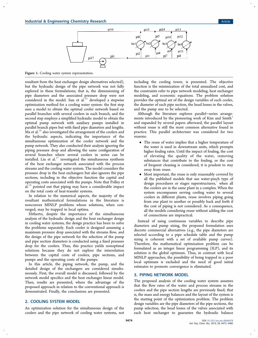
displayed in Tables 19−25. Tables 19−22 contain the designvariables of the heat exchangers; Table 23 displays thethermofluid dynamic behavior of heat exchanger he2 (thecorresponding results of the other heat exchangers are omittedto save space); Table 24 displays the optimal pump heads andvalve head losses, and Table 25 presents the objective functionand its corresponding components. The complete set of resultsof example 2 is available in the Supporting Information.Table 25 indicates a behavior of the two-step design A

approach similar to the previous example. The heat exchangercost is minimized according to the available pressure drop atthe expense of the operational costs, which results in a highertotal annualized cost.Unlike in the case of one exchanger, the two-step design B

approach yielded a solution associated with a higher totalannualized cost when compared with the simultaneoussolution. The optimization using the simultaneous approachand the two-step design problem B yielded heat exchangerswith the same area, with exception of heat exchanger he2, as isdisplayed in Tables 19−22. In relation of this heat exchanger,the simultaneous design selected an option with a larger area(Table 20, 246.6 m2 × 211.5 m2), but lower shell-side pressuredrop, where the cooling water flows (Table 23, 16.1 kPa × 36.6kPa). Despite the penalty of a more expensive heat exchanger,the analysis of the selected pumps for each case in Table 24indicates that this selection allowed the identification of anoptimal solution associated with a pump with lower power,which yielded a reduction of the operational costs, as can beobserved in Table 25. The optimization of the total annualizedcost of the heat exchangers separately in the two-step designproblem B penalized the operational costs, which implies ahigher value of the total annualized cost of the entire system.

Table 12. Example 1: Diameters and Head Losses of the Pipes

simultaneous design two-step design A two-step design B

pipe diameter (in) head loss (m) diameter(in) head loss (m) diameter(in) head loss (m)

pi1 8 2.329 8 2.329 8 2.329pi2 5 1.643 6 0.670 5 1.643pi3 6 0.670 6 0.670 6 0.670pi4 8 2.352 8 2.352 8 2.352pi5 8 0.024 8 0.024 8 0.024

Table 13. Example 1: Pump Head and Valve Head Loss

design pump head (m) valve head loss (m)

simultaneous design 10 0.032two-step design A 18 0.575two-step design B 10 0.032

Table 14. Example 1: Annualized Costs

cost ($/year)simultaneous

designtwo-stepdesign A

two-stepdesign B

pump cost 662.10 726.58 662.10heat exchanger cost 6080.93 5731.90 6080.93pipe cost 6154.28 6188.01 6154.28operation cost 5313.13 9563.64 5313.13total cost 18210.44 22210.13 18210.44

Table 15. Example 2: Pump Head Options

options

pump head (m) 6, 7, 10, 12, 14, 18, 20, 22, 25, 28, 30, 33, 35, 37, 40

Table 16. Example 2: Physical Properties of the Streams

hot stream

he1 he2 he3 he4

density (kg/m3) 1080 750 786 1080heat capacity (J/kg·K) 3601 2840 2177 3601viscosity (mPa·s) 1.3 0.34 1.89 1.30thermal conductivity (W/m·K) 0.58 0.19 0.12 0.58



9481

http://pubs.acs.org/doi/suppl/10.1021/acs.iecr.8b06478/suppl_file/ie8b06478_si_001.pdf


8. CONCLUSIONSThis paper presented a new approach for the design of coolingwater systems encompassing the dimensioning of coolers,pipes, and pumps. This approach allows the full exploration ofthe trade-off between capital and operational costs, includingall system elements simultaneously.Two examples were explored to analyze the comparison of

the proposed approach in relation to alternative schemes based

on the separation of the design of the coolers and the pipenetwork (two-step designs A and B).In the first example, the proposed approach yielded a better

result than the two-step approach based on the design of thecoolers through the area minimization constrained by pressuredrop bounds (two-step design A). However, the proposed

Table 17. Example 2: Cooling Tasks Data

he1 hot/cold he2 hot/cold he3 hot/cold he4 hot/cold

mass flow rate (kg/s) 21.94/75.48 27.8/56.57 30/77.99 14/36.12inlet temperature (°C) 90/30 70/30 100/30 80/30outlet temperature (°C) 50/40 40/40 50/40 50/40fouling factor (m2·K/W) 0.0001/0.0004 0.0002/0.0004 0.0002/0.0004 0.0001/0.0004allowable pressure drop (kPa) 100/100 70/50 60/100 100/50

Table 18. Example 2: Pipe lengths

pipe length (m) pipe length (m)

pi1 98 pi10 8pi2 12 pi11 10pi3 20 pi12 10pi4 15 pi13 18pi5 15 pi14 25pi6 12 pi15 20pi7 25 pi16 100pi8 18 pi17 2pi9 8


simultaneousdesign

two-stepdesign A

two-stepdesign B


2 4 2


677 781 677

baffle spacing (m) 0.191 0.163 0.160


simultaneousdesign

two-stepdesign A

two-stepdesign B


6 6 6


676 781 580

baffle spacing (m) 0.678 0.542 0.610


simultaneousdesign

two-stepdesign A

two-stepdesign B


2 4 2


677 1137 677

baffle spacing (m) 0.271 0.305 0.271


simultaneousdesign

two-stepdesign A

two-stepdesign B


2 4 2


344 419 677

baffle spacing (m) 0.229 0.136 0.261

Table 23. Example 2: Thermofluid Dynamic Results (he2)

simultaneousdesign

two-stepdesign A

two-stepdesign B

shell-side flow velocity(m/s)

0.570 0.712 0.734

tube-side flow velocity(m/s)

1.689 1.462 1.969

shell-side coefficient(W/m2 K)

3819.9 4980.4 5064.3

tube-side coefficient (W/m2 K)

3471.5 3092.8 3924.0

overall coefficient(W/m2 K)

776.2 787.4 844.7

shell-side pressure drop(Pa)

16106 35163 35587

tube-side pressure drop(Pa)

71172 45165 94475



9482


approach brought no additional gain in relation to the two-stepdesign based on the minimization of the total annualized costof the coolers followed by the minimization of the totalannualized cost of the pipe network (two-step design B).However, in the second example, the proposed approach

yielded better results than both two-step design approaches,illustrating potential gains that could be achieved when thedesign problem is addressed considering all elementssimultaneously. It seems that in the simultaneous approach, aheat exchanger could be chosen by the optimization to bebigger so that the corresponding pressure drop is lower, thusreducing the cost of pumping. The sequential approach cannothandle this trade-off.Because of the complexity of the chemical process design

problem, the traditional approach involves its solution in“layers”, where the solution of one layer is employed for theresolution of the next. If this conventional approach allows theanalysis of complex systems through a set of simpler problems,it may yield suboptimal solutions. In fact, this paper presentsone kind of system where a holistic design approach mayachieve better results, therefore reinforcing the need to useoptimization tools for the solution of chemical process designproblems.Finally, the design of the cooling water tower will certainly

include a new trade-off. For it to be considered, one also needsto take into account modifications in the return and supplytemperatures, the inclusion of the capital cost of the coolingtower, blow-down issues, and makeup water associated with itsoperational characteristics. This is the objective of future work.

■ ASSOCIATED CONTENT*S Supporting InformationThe Supporting Information is available free of charge on theACS Publications website at DOI: 10.1021/acs.iecr.8b06478.

Complete set of results of example 2 (PDF)

■ AUTHOR INFORMATIONCorresponding Author*E-mail: [email protected] J. Bagajewicz: 0000-0003-2195-0833Andre L. H. Costa: 0000-0001-9167-8754

NotesThe authors declare no competing financial interest.

■ ACKNOWLEDGMENTS

A.L.L.L. thanks the Coordination for the Improvement ofHigher Education Personnel (CAPES) for the doctoralfellowship. A.L.H.C. thanks the National Council for Scientificand Technological Development (CNPq) for the researchproductivity fellowship (Process 311225/2016-0) and the Riode Janeiro State University (UERJ) for the financial supportthrough the Prociencia Program.

■ NOMENCLATURE (PARAMETERS)

Aexc = excess area (%)c = Hazen−Williams parameterCPIn = annualized cost of a pipe section with unitary length(USD/y·m)Cpus= annualized capital cost of the pump alternative s

(USD/y)C = correlation parameter in eq 72,

Dnnom = nominal diameter of the commercial pipe n (in)

Dnint = inner diameter of the commercial pipe n (m)

Fsrow l, = correction factor of the LMTD for a configuration 1

− N, N evenFmp = cost factor related to the pump material

Fmhl= cost factor related to the heat exchanger (shell/tube)

materialFms = Marshall−Swift index correction factor, for the pumpcostFmseq = Marshall−Swift index correction factor, for the heatexchangers costFmspip = Marshall−Swift index correction factor, for thetubes costFphl = cost factor related to pressure range of the heat

exchangerFts= cost factor related to the pump type

g = gravity acceleration (m/s2)i = interest rateksl = thermal conductivity of the shell-side stream in thecooler l (W/(m K))ktl = thermal conductivity of the tube-side stream in the

cooler l (W/(m K))ktube = tube wall thermal conductivity (W/(m K))Lk = length of the pipe section k (m)

m = correlation parameter in eq 72

msl = shell-side mass flow rate in the cooler l (kg/s)mtl = tube-side mass flow rate in the cooler l (kg/s)Nop = number of operating hours per yearny = number of years of the project lifePl = LMTD correction factor parameter

pc = power cost (USD/kWh)PDeqsrow = equivalent diameter of the cooler alternative srow

(m)PDssrow = shell diameter of the cooler alternative srow (m)

Table 24. Example 2: Pump Head and Valve Head Losses

design

pumphead(m)

headloss−he1(m)

headloss−he2(m)

headloss−he3(m)

headloss−he4(m)

simultaneousdesign

6 0.450 0.017 0.024 0.027

two-stepdesign A

10 0.599 0.588 0.726 0.008

two-stepdesign B

10 2.522 0.102 0.259 0.033

Table 25. Example 2: Annualized Costs

cost ($/year)simultaneous

designtwo-stepdesign A

two-stepdesign B

pump cost 1455.21 1752.81 1752.81heat exchanger cost 48350.33 46232.95 46253.56pipe cost 15606.02 13591.52 12354.19operational cost 20739.07 34565.12 34565.12total cost 86150.64 96142.40 94925.69



9483

http://pubs.acs.org

http://pubs.acs.org/doi/abs/10.1021/acs.iecr.8b06478

http://pubs.acs.org/doi/suppl/10.1021/acs.iecr.8b06478/suppl_file/ie8b06478_si_001.pdf

mailto:[email protected]

http://orcid.org/0000-0003-2195-0833

http://orcid.org/0000-0001-9167-8754


Pdtesrow = outer tube diameter of the cooler alternative srow

(m)Pdtisrow = inner tube diameter of the cooler alternative srow

(m)pfkn= unitary head loss for a pipe diameter n in a pipe

section k (m/m)PLsrow = tube length of the cooler alternative srow (m)

Playsrow = tube layout of the cooler alternative srow

PNbsrow = number of baffles of the cooler alternative srow

PNpt srow = number of tube passes of the cooler alternative

srowPNttsrow = total number of tubes of the cooler alternative

srowPrpsrow = tube pitch ratio of the cooler alternative srow

qk = volumetric flow rate in the edge k (m3/s)

qhel = volumetric flow rate at the cooler related to the

hydraulic circuit l (m3/s)qpus

design = volumetric flow rate at the design condition ofthe pump s (m3/s)Q l = heat duty of the cooler l (W)

r = annualization factorRl = LMTD correction factor parameter

Rf s = shell-side fouling factor (m2 K/W)

Rf t = tube-side fouling factor (m2 K/W)vmax = maximum flow velocity in the pipe sectionsvmin = minimum flow velocity in the pipe sectionsvsmax = maximum flow velocity in the heat exchanger shell-sidevsmin = minimum flow velocity in the heat exchanger shell-sidevtmax = maximum flow velocity in the heat exchanger tube-sidevtmin = minimum flow velocity in the heat exchanger tube-sideyT c l,

= binary parameter, if the cooling water is in the tube-

side (yT 1c l, = )

yTh l, = binary parameter, if the hot process stream is in the

tube-side (yT 1h l, = )

zs = parameter for the calculation of pump capital cost in eq74

PsdisplΔ = shell-side available pressure drop in the cooler l(Pa)

PtdisplΔ = tube-side available pressure drop in the cooler l(Pa)

TlmlΔ = log-mean temperature difference of the cooler l(°C)

zΔ = elevation difference between top and bottom of thecooling tower (m)η = pump efficiency

lkΛ = circuit matrixslμ = viscosity of the shell-side stream in the cooler l (Pa·s)tlμ = viscosity of the tube-side stream in the cooler l (Pa·s)

slρ = density of the shell-side stream in the cooler l (kg/m3)tlρ = density (kg/m3)

wρ = water density (kg/m3)

■ BINARY VARIABLESyk,n

pi = binary variable, if the commercial diameter n is in theedge k, so yk,n

pi = 1yk,s

pu = binary variable, if the pump s is in the edge k, so yk,spu

= 1yrowsrow,l = variable representing the set of heat exchangerdesign variables

■ CONTINUOUS AND DISCRETE VARIABLESA = heat-transfer area (m2)C = objective function (USD/y)copk = operating cost of pump k (USD/y)Cheatexch = annualized capital cost of the heat exchangers(USD/y)Coper = pipe network operating cost (USD/y)Cpipe = annualized capital cost of the pipe sections (USD/y)Cpump = annualized capital cost of the pump (USD/y)Dk = inner diameter of the pipe section k (m)dte = outer tube diameter (m)dti = outer tube diameter (m)Ds = shell diameter (m)f k = unitary head loss along pipe sections k (dimensionless)fhel = head loss in the cooler l (m)fpik = head loss in the pipe section k (m)fpuk = head of the pump k (m)f vl = head loss in the valve l (m)hs = shell-side convective heat-transfer coefficient (W/m2

K)ht = tube-side convective heat-transfer coefficient (W/m2 K)L = heat exchanger tube length (m)Lk = tube length in the pipe section k (m)lay = tube layout (1 = square, 2 = triangular)lbc = baffle spacing (m)Nb = number of bafflesNpt = number of passes in the tube-sideNtt = total number of tubesRes = shell-side Reynolds numberRet = tube-side Reynolds numberrp = tube pitch ratioU = overall heat-transfer coefficient (W/m2 K)vk = flow velocity in pipe section k (m/s)vs = shell-side flow velocity (m/s)vt = tube-side flow velocity (m/s)ΔPt = tube-side pressure drop (Pa)ΔPs = shell-side pressure drop (Pa)

■ SETSHE = subset of heat exchangersHY = set of hydraulic circuitsINT = node subset of interconnectionsPD = water return node subsetPI = subset of pipe sectionsPS = water supply node subsetPU = subset of the pumpsSD = set of commercial diametersSPU = set of available pumpsSTR = set of edgesVET = set of nodes



9484


■ SUBSCRIPTSk = index of the edgesl = index of the hydraulic circuitsn = index of commercial diameterss = index of the available pump alternativest = index of the nodes

■ SUPERSCRIPTSdesign = design conditionint = internalnom = nominalpi = pipepu = pump

■ REFERENCES(1) Kim, J.; Smith, R. Cooling water system design. Chem. Eng. Sci.2001, 56, 3641.(2) Kim, J.; Smith, R. Automated retrofit design of cooling-watersystems. AIChE J. 2003, 49, 1712.(3) Kim, J.; Lee, G. C.; Zhu, F. X. X.; Smith, R. Cooling systemdesign. Heat Transfer Eng. 2002, 23, 49.(4) Feng, X.; Shen, R. J.; Wang, B. Recirculating cooling-waternetwork with an intermediate cooling-water main. Energy Fuels 2005,19, 1723.(5) Picon-Nunez, M.; Morales-Fuentes, A.; Vazquez-Ramírez, E. E.Effect of network arrangement on the heat Transfer area of coolingnetworks. Appl. Therm. Eng. 2007, 27, 2650.(6) Ponce-Ortega, J. M.; Serna-Gonzalez, M.; Jimenez-Gutierrez, A.MINLP synthesis of optimal cooling networks. Chem. Eng. Sci. 2007,62, 5728.(7) Yee, T. F.; Grossmann, I. E. Simultaneous optimization modelsfor heat integration − II. Heat exchanger network synthesis. Comput.Chem. Eng. 1990, 14, 1165.(8) Picon-Nunez, M.; Polley, G. T.; Canizalez-Davalos, L.; Medina-Flores, J. M. Short cut performance method for the design of flexiblecooling systems. Energy 2011, 36, 4646.(9) Pico n-Nu nez, M.; Polley, G. T.; Canizalez-Davalos, L.;Tamakloe, E. K. Design of coolers for use in an existing coolingwater network. Appl. Therm. Eng. 2012, 43, 51.(10) Sun, J.; Feng, X.; Wang, Y.; Deng, C.; Chu, K. H. Pumpnetwork optimization for a cooling water system. Energy 2014, 67,506.(11) De Souza, J. N. M.; Ventin, F. F.; Tavares, V. B. G.; Costa, A. L.H. A matrix approach for optimization of pipenetworks in coolingwater systems. Chem. Eng. Commun. 2014, 201, 1054.(12) Souza, J. N. M.; Levy, A. L. L.; Costa, A. L. H. Optimization ofcooling water system hydraulic debottlenecking. Appl. Therm. Eng.2018, 128, 1531.(13) Ponce-Ortega, J. M.; Serna-Gonzalez, M.; Jimenez-Gutierrez, A.A Disjunctive Programming Model for Simultaneous Synthesis andDetailedDesign of CoolingNetworks. Ind. Eng. Chem. Res. 2009, 48,2991.(14) Ponce-Ortega, J. M.; Serna-Gonzalez, M.; Jimenez-Gutierrez, A.Optimization model for re-circulatingcooling water systems. Comput.Chem. Eng. 2010, 34, 177.(15) Sun, J.; Feng, X.; Wang, Y. Cooling-water system optimizationwith a novel two-step sequentialmethod. Appl. Therm. Eng. 2015, 89,1006.(16) Ma, J.; Wang, Y.; Feng, X. Simultaneous optimization of pumpand cooler networks in a coolingwater system. Appl. Therm. Eng.2017, 125, 377.(17) Liu, F.; Ma, J.; Feng, X.; Wang, Y. Simultaneous integrateddesign for heat exchanger network and coolingwater system. Appl.Therm. Eng. 2018, 128, 1510.(18) Polley, G. T.; Picon-Nunez, M.; Lopez-Maciel, J. J. Design ofwater and heat recovery networks for the simultaneous minimizationof water and energy consumption. Appl. Therm. Eng. 2010, 30, 2290.

(19) Mah, R. S. H. Chemical Process Structures and Information Flows;Butterworth Publishers: Markham, 1990.(20) Goncalves, C. O.; Costa, A. L. H.; Bagajewicz, M. J. Alternativemixed-integer linear programming formulations for shell and tubeheat exchanger optimal design. Ind. Eng. Chem. Res. 2017, 56, 5970.(21) Kakac, S.; Liu, H. Heat Exchangers Selection, Rating, andThermal Design; CRC Press: Boca Raton, FL, 2002.(22) Incropera, F. P.; De Witt, D. P. Fundamentals of Heat and MassTransfer; John Wiley & Sons: New York, 2002.(23) Kern, D. Q. Process Heat Transfer; McGraw-Hill: New York,1950.(24) Saunders, E. A. D. Heat Exchangers: Selection, Design, andConstruction; John Wiley & Sons: New York, 1988.(25) Taborek, J. Input Data and Recommended Practices. In HeatExchanger Design Handbook; Hewitt, G. F., Ed.; Begell House:NewYork, 2008.(26) Souza, P. A.; Costa, A. L. H.; Bagajewicz, M. J. Globally optimallinear approach for the design of process equipment: The case of aircoolers. AIChE J. 2018, 64, 886.(27) Narang, R.; Sarin, S.; George, A. A. De-emphasize capital costsfor pipe size selection. Chem. Eng. 2009, 116, 41.(28) Couper, J. R.; Penney, W. R.; Fair, J. R.; Walas, S. M. ChemicalProcess Equipment:Selection and Design.; Gulf Professional Publishing:MA, 2005.



9485


Documents

Globally Optimal Design Optimization of Cooling Water Systems