Embed Size (px)
Citation preview
GMMAT: Generalized linear Mixed ModelAssociation TestsVersion 1.2.0
Han ChenHuman Genetics Center
Dept. of Epidemiology, Human Genetics and Environmental SciencesCenter for Precision Health
School of Public Health & School of Biomedical InformaticsThe University of Texas Health Science Center at Houston
Email: [email protected]
May 14, 2020
1
Contents
1 Introduction 4
2 The model 4
3 Getting started 63.1 Downloading GMMAT . . . . . . . . . . . . . . . . . . . . . . . . . . . . 63.2 Installing GMMAT . . . . . . . . . . . . . . . . . . . . . . . . . . . . . . 63.3 Using GMMAT in Analysis Commons . . . . . . . . . . . . . . . . . . . 7
4 Input 74.1 Phenotype and covariates . . . . . . . . . . . . . . . . . . . . . . . . . . 74.2 Matrices of covariance structure . . . . . . . . . . . . . . . . . . . . . . . 84.3 Genotypes . . . . . . . . . . . . . . . . . . . . . . . . . . . . . . . . . . . 8
5 Running GMMAT 95.1 Fitting GLMM . . . . . . . . . . . . . . . . . . . . . . . . . . . . . . . . 95.2 Single variant tests . . . . . . . . . . . . . . . . . . . . . . . . . . . . . . 13
5.2.1 Score tests . . . . . . . . . . . . . . . . . . . . . . . . . . . . . . . 135.2.2 Wald tests . . . . . . . . . . . . . . . . . . . . . . . . . . . . . . . 145.2.3 Meta-analysis . . . . . . . . . . . . . . . . . . . . . . . . . . . . . 16
5.3 Variant set tests . . . . . . . . . . . . . . . . . . . . . . . . . . . . . . . . 165.3.1 Pooled analysis . . . . . . . . . . . . . . . . . . . . . . . . . . . . 165.3.2 Meta-analysis . . . . . . . . . . . . . . . . . . . . . . . . . . . . . 19
6 Output 19
7 Advanced options 227.1 Alternative model fitting algorithms . . . . . . . . . . . . . . . . . . . . . 227.2 Changing model fitting parameters . . . . . . . . . . . . . . . . . . . . . 227.3 Missing genotypes . . . . . . . . . . . . . . . . . . . . . . . . . . . . . . . 237.4 Reordered genotypes . . . . . . . . . . . . . . . . . . . . . . . . . . . . . 237.5 Parallel computing . . . . . . . . . . . . . . . . . . . . . . . . . . . . . . 237.6 Variant filters . . . . . . . . . . . . . . . . . . . . . . . . . . . . . . . . . 247.7 Internal minor allele frequency weights . . . . . . . . . . . . . . . . . . . 247.8 Allele flipping . . . . . . . . . . . . . . . . . . . . . . . . . . . . . . . . . 247.9 P values of weighted sum of chi-squares . . . . . . . . . . . . . . . . . . . 257.10 Heterogeneous genetic effects in variant set meta-analysis . . . . . . . . . 257.11 Other options . . . . . . . . . . . . . . . . . . . . . . . . . . . . . . . . . 25
8 Version 268.1 Version 0.6 (October 12, 2015) . . . . . . . . . . . . . . . . . . . . . . . . 268.2 Version 0.7 (January 22, 2016) . . . . . . . . . . . . . . . . . . . . . . . . 268.3 Version 0.7-1 (January 22, 2016) . . . . . . . . . . . . . . . . . . . . . . . 268.4 Version 0.9 (March 9, 2018) . . . . . . . . . . . . . . . . . . . . . . . . . 268.5 Version 0.9.1 (May 13, 2018) . . . . . . . . . . . . . . . . . . . . . . . . . 278.6 Version 0.9.2 (June 8, 2018) . . . . . . . . . . . . . . . . . . . . . . . . . 278.7 Version 0.9.3 (July 18, 2018) . . . . . . . . . . . . . . . . . . . . . . . . . 27
2

8.8 Version 1.0.0 (December 28, 2018) . . . . . . . . . . . . . . . . . . . . . . 288.9 Version 1.0.1 (January 1, 2019) . . . . . . . . . . . . . . . . . . . . . . . 288.10 Version 1.0.2 (January 2, 2019) . . . . . . . . . . . . . . . . . . . . . . . 298.11 Version 1.0.3 (January 14, 2019) . . . . . . . . . . . . . . . . . . . . . . . 298.12 Version 1.0.4 (March 6, 2019) . . . . . . . . . . . . . . . . . . . . . . . . 298.13 Version 1.1.0 (May 21, 2019) . . . . . . . . . . . . . . . . . . . . . . . . . 298.14 Version 1.1.1 (August 26, 2019) . . . . . . . . . . . . . . . . . . . . . . . 298.15 Version 1.1.2 (October 11, 2019) . . . . . . . . . . . . . . . . . . . . . . . 298.16 Version 1.2.0 (May 14, 2020) . . . . . . . . . . . . . . . . . . . . . . . . . 29
9 Contact 30
10 Acknowledgments 30
3
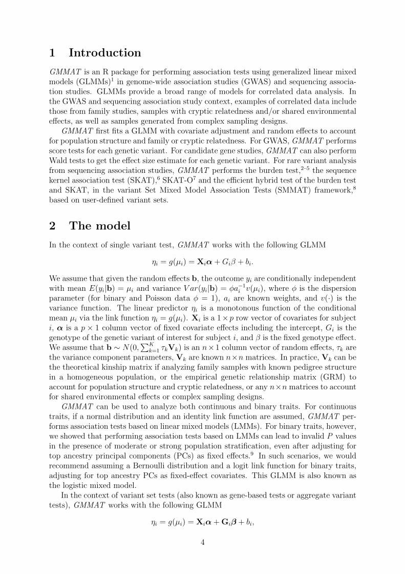
1 Introduction
GMMAT is an R package for performing association tests using generalized linear mixedmodels (GLMMs)1 in genome-wide association studies (GWAS) and sequencing associa-tion studies. GLMMs provide a broad range of models for correlated data analysis. Inthe GWAS and sequencing association study context, examples of correlated data includethose from family studies, samples with cryptic relatedness and/or shared environmentaleffects, as well as samples generated from complex sampling designs.
GMMAT first fits a GLMM with covariate adjustment and random effects to accountfor population structure and family or cryptic relatedness. For GWAS, GMMAT performsscore tests for each genetic variant. For candidate gene studies, GMMAT can also performWald tests to get the effect size estimate for each genetic variant. For rare variant analysisfrom sequencing association studies, GMMAT performs the burden test,2–5 the sequencekernel association test (SKAT),6 SKAT-O7 and the efficient hybrid test of the burden testand SKAT, in the variant Set Mixed Model Association Tests (SMMAT) framework,8
based on user-defined variant sets.
2 The model
In the context of single variant test, GMMAT works with the following GLMM
ηi = g(µi) = Xiα+Giβ + bi.
We assume that given the random effects b, the outcome yi are conditionally independentwith mean E(yi|b) = µi and variance V ar(yi|b) = φa−1
i v(µi), where φ is the dispersionparameter (for binary and Poisson data φ = 1), ai are known weights, and v(·) is thevariance function. The linear predictor ηi is a monotonous function of the conditionalmean µi via the link function ηi = g(µi). Xi is a 1×p row vector of covariates for subjecti, α is a p × 1 column vector of fixed covariate effects including the intercept, Gi is thegenotype of the genetic variant of interest for subject i, and β is the fixed genotype effect.We assume that b ∼ N(0,
∑Kk=1 τkVk) is an n×1 column vector of random effects, τk are
the variance component parameters, Vk are known n×n matrices. In practice, Vk can bethe theoretical kinship matrix if analyzing family samples with known pedigree structurein a homogeneous population, or the empirical genetic relationship matrix (GRM) toaccount for population structure and cryptic relatedness, or any n×n matrices to accountfor shared environmental effects or complex sampling designs.
GMMAT can be used to analyze both continuous and binary traits. For continuoustraits, if a normal distribution and an identity link function are assumed, GMMAT per-forms association tests based on linear mixed models (LMMs). For binary traits, however,we showed that performing association tests based on LMMs can lead to invalid P valuesin the presence of moderate or strong population stratification, even after adjusting fortop ancestry principal components (PCs) as fixed effects.9 In such scenarios, we wouldrecommend assuming a Bernoulli distribution and a logit link function for binary traits,adjusting for top ancestry PCs as fixed-effect covariates. This GLMM is also known asthe logistic mixed model.
In the context of variant set tests (also known as gene-based tests or aggregate varianttests), GMMAT works with the following GLMM
ηi = g(µi) = Xiα+ Giβ + bi,
4
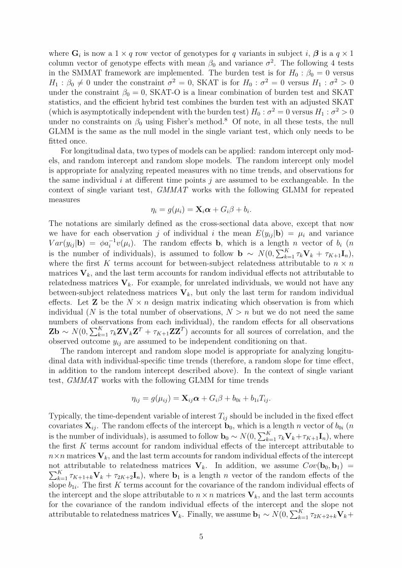
where Gi is now a 1× q row vector of genotypes for q variants in subject i, β is a q × 1column vector of genotype effects with mean β0 and variance σ2. The following 4 testsin the SMMAT framework are implemented. The burden test is for H0 : β0 = 0 versusH1 : β0 6= 0 under the constraint σ2 = 0, SKAT is for H0 : σ2 = 0 versus H1 : σ2 > 0under the constraint β0 = 0, SKAT-O is a linear combination of burden test and SKATstatistics, and the efficient hybrid test combines the burden test with an adjusted SKAT(which is asymptotically independent with the burden test) H0 : σ2 = 0 versus H1 : σ2 > 0under no constraints on β0 using Fisher’s method.8 Of note, in all these tests, the nullGLMM is the same as the null model in the single variant test, which only needs to befitted once.
For longitudinal data, two types of models can be applied: random intercept only mod-els, and random intercept and random slope models. The random intercept only modelis appropriate for analyzing repeated measures with no time trends, and observations forthe same individual i at different time points j are assumed to be exchangeable. In thecontext of single variant test, GMMAT works with the following GLMM for repeatedmeasures
ηi = g(µi) = Xiα+Giβ + bi.
The notations are similarly defined as the cross-sectional data above, except that nowwe have for each observation j of individual i the mean E(yij|b) = µi and varianceV ar(yij|b) = φa−1
i v(µi). The random effects b, which is a length n vector of bi (n
is the number of individuals), is assumed to follow b ∼ N(0,∑K
k=1 τkVk + τK+1In),where the first K terms account for between-subject relatedness attributable to n × nmatrices Vk, and the last term accounts for random individual effects not attributable torelatedness matrices Vk. For example, for unrelated individuals, we would not have anybetween-subject relatedness matrices Vk, but only the last term for random individualeffects. Let Z be the N × n design matrix indicating which observation is from whichindividual (N is the total number of observations, N > n but we do not need the samenumbers of observations from each individual), the random effects for all observationsZb ∼ N(0,
∑Kk=1 τkZVkZ
T + τK+1ZZT ) accounts for all sources of correlation, and theobserved outcome yij are assumed to be independent conditioning on that.
The random intercept and random slope model is appropriate for analyzing longitu-dinal data with individual-specific time trends (therefore, a random slope for time effect,in addition to the random intercept described above). In the context of single varianttest, GMMAT works with the following GLMM for time trends
ηij = g(µij) = Xijα+Giβ + b0i + b1iTij.
Typically, the time-dependent variable of interest Tij should be included in the fixed effectcovariates Xij. The random effects of the intercept b0, which is a length n vector of b0i (n
is the number of individuals), is assumed to follow b0 ∼ N(0,∑K
k=1 τkVk+τK+1In), wherethe first K terms account for random individual effects of the intercept attributable ton×n matrices Vk, and the last term accounts for random individual effects of the interceptnot attributable to relatedness matrices Vk. In addition, we assume Cov(b0,b1) =∑K
k=1 τK+1+kVk + τ2K+2In), where b1 is a length n vector of the random effects of theslope b1i. The first K terms account for the covariance of the random individual effects ofthe intercept and the slope attributable to n×n matrices Vk, and the last term accountsfor the covariance of the random individual effects of the intercept and the slope notattributable to relatedness matrices Vk. Finally, we assume b1 ∼ N(0,
∑Kk=1 τ2K+2+kVk+
5
τ3K+3In), where the first K terms account for random individual effects of the slopeattributable to n×n matrices Vk, and the last term accounts for random individual effectsof the slope not attributable to relatedness matrices Vk. For example, with K = 1, letb = (bT
0 ,bT1 )T be the stacked random individual effects (for both the intercept and the
slope), Z be the N × 2n design matrix for linking observations with their correspondingrandom intercept and random slope (N is the total number of observations, again we donot need the same numbers of observations from each individual), the random effects for
all observations Zb ∼ N(0,Z{(τ1 τ3τ3 τ5
)⊗Vk+
(τ2 τ4τ4 τ6
)⊗In}ZT ) accounts for all sources
of correlation, and the observed outcome yij are assumed to be independent conditioningon that.
Variant set tests for longitudinal data in the SMMAT framework are similarly defined,for both random intercept only models (repeated, exchangeable measures), and randomintercept and random slope models (time trends).
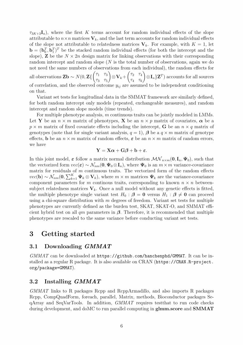
For multiple phenotype analysis, m continuous traits can be jointly modeled in LMMs.Let Y be an n ×m matrix of phenotypes, X be an n × p matrix of covariates, α be ap ×m matrix of fixed covariate effects including the intercept, G be an n × q matrix ofgenotypes (note that for single variant analysis, q = 1), β be a q×m matrix of genotypeeffects, b be an n×m matrix of random effects, ε be an n×m matrix of random errors,we have
Y = Xα+ Gβ + b + ε.
In this joint model, ε follow a matrix normal distribution MN n×m(0, In,Ψ0), such thatthe vectorized form vec(ε) ∼ Nnm(0,Ψ0⊗ In), where Ψ0 is an m×m variance-covariancematrix for residuals of m continuous traits. The vectorized form of the random effectsvec(b) ∼ Nnm(0,
∑Kk=1 Ψk ⊗Vk), where m×m matrices Ψk are the variance-covariance
component parameters for m continous traits, corresponding to known n × n between-subject relatedness matrices Vk. Once a null model without any genetic effects is fitted,the multiple phenotype single variant test H0 : β = 0 versus H1 : β 6= 0 can proceedusing a chi-square distribution with m degrees of freedom. Variant set tests for multiplephenotypes are currently defined as the burden test, SKAT, SKAT-O, and SMMAT effi-cient hybrid test on all qm parameters in β. Therefore, it is recommended that multiplephenotypes are rescaled to the same variance before conducting variant set tests.
3 Getting started
3.1 Downloading GMMAT
GMMAT can be downloaded at https://github.com/hanchenphd/GMMAT. It can be in-stalled as a regular R package. It is also available on CRAN (https://CRAN.R-project.org/package=GMMAT).
3.2 Installing GMMAT
GMMAT links to R packages Rcpp and RcppArmadillo, and also imports R packagesRcpp, CompQuadForm, foreach, parallel, Matrix, methods, Bioconductor packages Se-qArray and SeqVarTools. In addition, GMMAT requires testthat to run code checksduring development, and doMC to run parallel computing in glmm.score and SMMAT
6
for genotype files in the GDS format (however, doMC is not available on Windows andthese functions will switch to a single thread). These dependencies should be installedbefore installing GMMAT.
For optimal computational performance, it is recommended to use an R version con-figured with the Intel Math Kernel Library (or other fast BLAS/LAPACK libraries). Seethe instructions on building R with Intel MKL (https://software.intel.com/en-us/articles/using-intel-mkl-with-r).
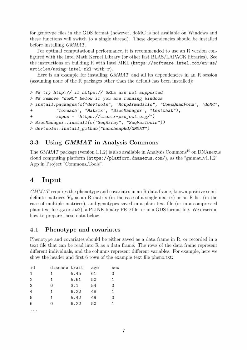
Here is an example for installing GMMAT and all its dependencies in an R session(assuming none of the R packages other than the default has been installed):
> ## try http:// if https:// URLs are not supported
> ## remove "doMC" below if you are running Windows
> install.packages(c("devtools", "RcppArmadillo", "CompQuadForm", "doMC",
+ "foreach", "Matrix", "BiocManager", "testthat"),
+ repos = "https://cran.r-project.org/")
> BiocManager::install(c("SeqArray", "SeqVarTools"))
> devtools::install_github("hanchenphd/GMMAT")
3.3 Using GMMAT in Analysis Commons
The GMMAT package (version 1.1.2) is also available in Analysis Commons10 on DNAnexuscloud computing platform (https://platform.dnanexus.com/), as the ”gmmat v1.1.2”App in Project ”Commons Tools”.
4 Input
GMMAT requires the phenotype and covariates in an R data frame, known positive semi-definite matrices Vk as an R matrix (in the case of a single matrix) or an R list (in thecase of multiple matrices), and genotypes saved in a plain text file (or in a compressedplain text file .gz or .bz2), a PLINK binary PED file, or in a GDS format file. We describehow to prepare these data below.
4.1 Phenotype and covariates
Phenotype and covariates should be either saved as a data frame in R, or recorded in atext file that can be read into R as a data frame. The rows of the data frame representdifferent individuals, and the columns represent different variables. For example, here weshow the header and first 6 rows of the example text file pheno.txt:
id disease trait age sex
1 1 5.45 61 0
2 1 5.61 50 1
3 0 3.1 54 0
4 1 6.22 48 1
5 1 5.42 49 0
6 0 6.22 50 1
...
7
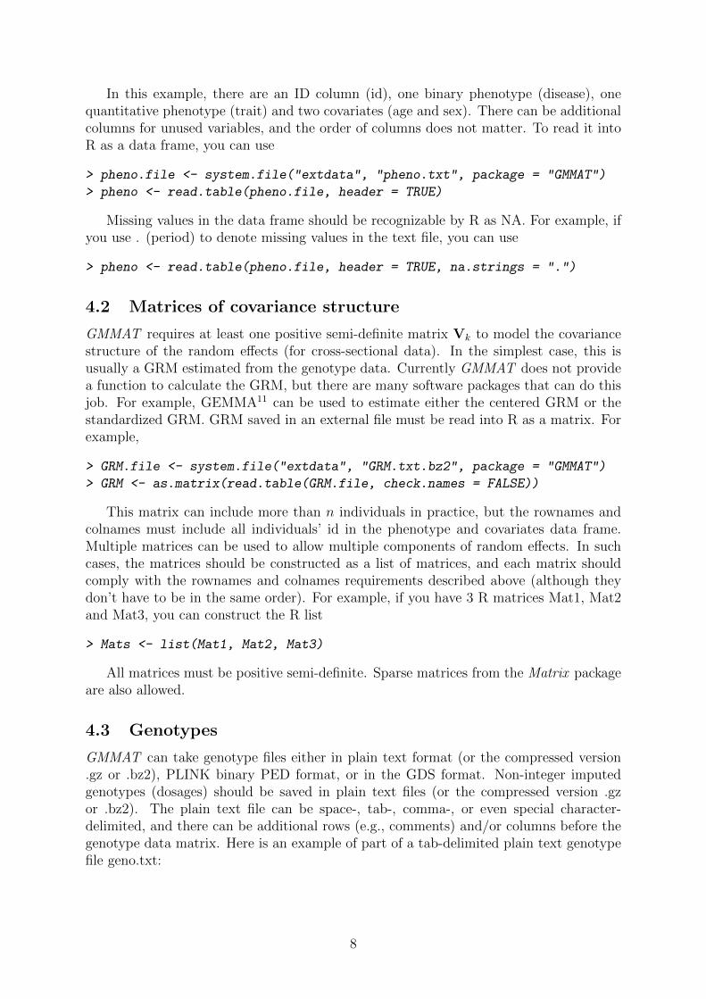
In this example, there are an ID column (id), one binary phenotype (disease), onequantitative phenotype (trait) and two covariates (age and sex). There can be additionalcolumns for unused variables, and the order of columns does not matter. To read it intoR as a data frame, you can use
> pheno.file <- system.file("extdata", "pheno.txt", package = "GMMAT")
> pheno <- read.table(pheno.file, header = TRUE)
Missing values in the data frame should be recognizable by R as NA. For example, ifyou use . (period) to denote missing values in the text file, you can use
> pheno <- read.table(pheno.file, header = TRUE, na.strings = ".")
4.2 Matrices of covariance structure
GMMAT requires at least one positive semi-definite matrix Vk to model the covariancestructure of the random effects (for cross-sectional data). In the simplest case, this isusually a GRM estimated from the genotype data. Currently GMMAT does not providea function to calculate the GRM, but there are many software packages that can do thisjob. For example, GEMMA11 can be used to estimate either the centered GRM or thestandardized GRM. GRM saved in an external file must be read into R as a matrix. Forexample,
> GRM.file <- system.file("extdata", "GRM.txt.bz2", package = "GMMAT")
> GRM <- as.matrix(read.table(GRM.file, check.names = FALSE))
This matrix can include more than n individuals in practice, but the rownames andcolnames must include all individuals’ id in the phenotype and covariates data frame.Multiple matrices can be used to allow multiple components of random effects. In suchcases, the matrices should be constructed as a list of matrices, and each matrix shouldcomply with the rownames and colnames requirements described above (although theydon’t have to be in the same order). For example, if you have 3 R matrices Mat1, Mat2and Mat3, you can construct the R list
> Mats <- list(Mat1, Mat2, Mat3)
All matrices must be positive semi-definite. Sparse matrices from the Matrix packageare also allowed.
4.3 Genotypes
GMMAT can take genotype files either in plain text format (or the compressed version.gz or .bz2), PLINK binary PED format, or in the GDS format. Non-integer imputedgenotypes (dosages) should be saved in plain text files (or the compressed version .gzor .bz2). The plain text file can be space-, tab-, comma-, or even special character-delimited, and there can be additional rows (e.g., comments) and/or columns before thegenotype data matrix. Here is an example of part of a tab-delimited plain text genotypefile geno.txt:
8
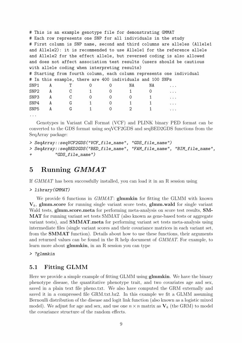
# This is an example genotype file for demonstrating GMMAT
# Each row represents one SNP for all individuals in the study
# First column is SNP name, second and third columns are alleles (Allele1
and Allele2): it is recommended to use Allele1 for the reference allele
and Allele2 for the effect allele, but reversed coding is also allowed
and does not affect association test results (users should be cautious
with allele coding when interpreting results)
# Starting from fourth column, each column represents one individual
# In this example, there are 400 individuals and 100 SNPs
SNP1 A T 0 0 NA NA ...
SNP2 A C 1 0 1 0 ...
SNP3 A C 0 0 0 1 ...
SNP4 A G 1 0 1 1 ...
SNP5 A G 1 0 2 1 ...
...
Genotypes in Variant Call Format (VCF) and PLINK binary PED format can beconverted to the GDS format using seqVCF2GDS and seqBED2GDS functions from theSeqArray package:
> SeqArray::seqVCF2GDS("VCF_file_name", "GDS_file_name")
> SeqArray::seqBED2GDS("BED_file_name", "FAM_file_name", "BIM_file_name",
+ "GDS_file_name")
5 Running GMMAT
If GMMAT has been successfully installed, you can load it in an R session using
> library(GMMAT)
We provide 6 functions in GMMAT : glmmkin for fitting the GLMM with knownVk, glmm.score for running single variant score tests, glmm.wald for single variantWald tests, glmm.score.meta for performing meta-analysis on score test results, SM-MAT for running variant set tests SMMAT (also known as gene-based tests or aggregatevariant tests), and SMMAT.meta for performing variant set tests meta-analysis usingintermediate files (single variant scores and their covariance matrices in each variant set,from the SMMAT function). Details about how to use these functions, their argumentsand returned values can be found in the R help document of GMMAT. For example, tolearn more about glmmkin, in an R session you can type
> ?glmmkin
5.1 Fitting GLMM
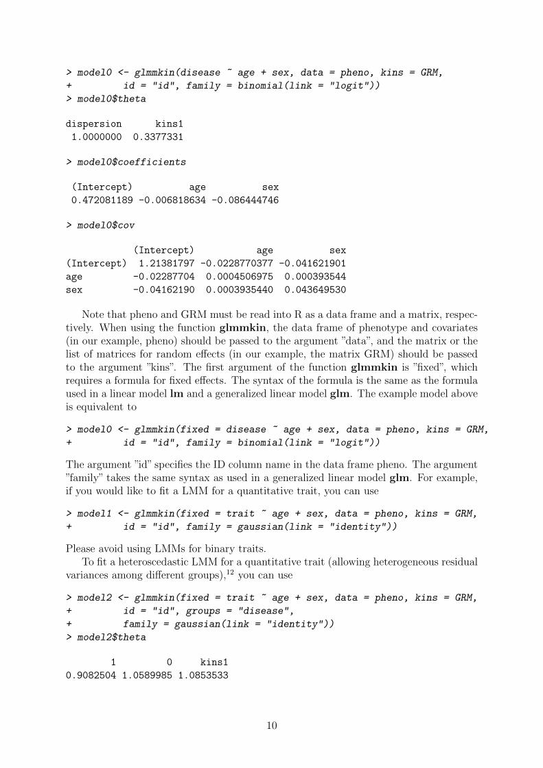
Here we provide a simple example of fitting GLMM using glmmkin. We have the binaryphenotype disease, the quantitative phenotype trait, and two covariates age and sex,saved in a plain text file pheno.txt. We also have computed the GRM externally andsaved it in a compressed file GRM.txt.bz2. In this example we fit a GLMM assumingBernoulli distribution of the disease and logit link function (also known as a logistic mixedmodel). We adjust for age and sex, and use one n×n matrix as Vk (the GRM) to modelthe covariance structure of the random effects.
9
> model0 <- glmmkin(disease ~ age + sex, data = pheno, kins = GRM,
+ id = "id", family = binomial(link = "logit"))
> model0$theta
dispersion kins1
1.0000000 0.3377331
> model0$coefficients
(Intercept) age sex
0.472081189 -0.006818634 -0.086444746
> model0$cov
(Intercept) age sex
(Intercept) 1.21381797 -0.0228770377 -0.041621901
age -0.02287704 0.0004506975 0.000393544
sex -0.04162190 0.0003935440 0.043649530
Note that pheno and GRM must be read into R as a data frame and a matrix, respec-tively. When using the function glmmkin, the data frame of phenotype and covariates(in our example, pheno) should be passed to the argument ”data”, and the matrix or thelist of matrices for random effects (in our example, the matrix GRM) should be passedto the argument ”kins”. The first argument of the function glmmkin is ”fixed”, whichrequires a formula for fixed effects. The syntax of the formula is the same as the formulaused in a linear model lm and a generalized linear model glm. The example model aboveis equivalent to
> model0 <- glmmkin(fixed = disease ~ age + sex, data = pheno, kins = GRM,
+ id = "id", family = binomial(link = "logit"))
The argument ”id” specifies the ID column name in the data frame pheno. The argument”family” takes the same syntax as used in a generalized linear model glm. For example,if you would like to fit a LMM for a quantitative trait, you can use
> model1 <- glmmkin(fixed = trait ~ age + sex, data = pheno, kins = GRM,
+ id = "id", family = gaussian(link = "identity"))
Please avoid using LMMs for binary traits.To fit a heteroscedastic LMM for a quantitative trait (allowing heterogeneous residual
variances among different groups),12 you can use
> model2 <- glmmkin(fixed = trait ~ age + sex, data = pheno, kins = GRM,
+ id = "id", groups = "disease",
+ family = gaussian(link = "identity"))
> model2$theta
1 0 kins1
0.9082504 1.0589985 1.0853533
10
In this example, groups are defined by disease status. Therefore, disease cases and controlsare assumed to have different residual variances on the quantitative trait, after adjustingfor age and sex.
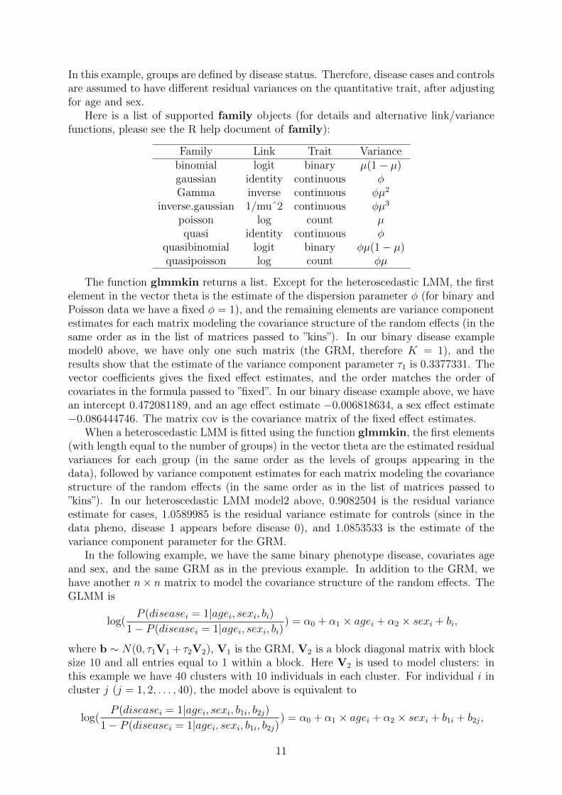
Here is a list of supported family objects (for details and alternative link/variancefunctions, please see the R help document of family):
Family Link Trait Variancebinomial logit binary µ(1− µ)gaussian identity continuous φGamma inverse continuous φµ2
inverse.gaussian 1/muˆ2 continuous φµ3
poisson log count µquasi identity continuous φ
quasibinomial logit binary φµ(1− µ)quasipoisson log count φµ
The function glmmkin returns a list. Except for the heteroscedastic LMM, the firstelement in the vector theta is the estimate of the dispersion parameter φ (for binary andPoisson data we have a fixed φ = 1), and the remaining elements are variance componentestimates for each matrix modeling the covariance structure of the random effects (in thesame order as in the list of matrices passed to ”kins”). In our binary disease examplemodel0 above, we have only one such matrix (the GRM, therefore K = 1), and theresults show that the estimate of the variance component parameter τ1 is 0.3377331. Thevector coefficients gives the fixed effect estimates, and the order matches the order ofcovariates in the formula passed to ”fixed”. In our binary disease example above, we havean intercept 0.472081189, and an age effect estimate −0.006818634, a sex effect estimate−0.086444746. The matrix cov is the covariance matrix of the fixed effect estimates.
When a heteroscedastic LMM is fitted using the function glmmkin, the first elements(with length equal to the number of groups) in the vector theta are the estimated residualvariances for each group (in the same order as the levels of groups appearing in thedata), followed by variance component estimates for each matrix modeling the covariancestructure of the random effects (in the same order as in the list of matrices passed to”kins”). In our heteroscedastic LMM model2 above, 0.9082504 is the residual varianceestimate for cases, 1.0589985 is the residual variance estimate for controls (since in thedata pheno, disease 1 appears before disease 0), and 1.0853533 is the estimate of thevariance component parameter for the GRM.
In the following example, we have the same binary phenotype disease, covariates ageand sex, and the same GRM as in the previous example. In addition to the GRM, wehave another n× n matrix to model the covariance structure of the random effects. TheGLMM is
log(P (diseasei = 1|agei, sexi, bi)
1− P (diseasei = 1|agei, sexi, bi)) = α0 + α1 × agei + α2 × sexi + bi,
where b ∼ N(0, τ1V1 + τ2V2), V1 is the GRM, V2 is a block diagonal matrix with blocksize 10 and all entries equal to 1 within a block. Here V2 is used to model clusters: inthis example we have 40 clusters with 10 individuals in each cluster. For individual i incluster j (j = 1, 2, . . . , 40), the model above is equivalent to
log(P (diseasei = 1|agei, sexi, b1i, b2j)
1− P (diseasei = 1|agei, sexi, b1i, b2j)) = α0 + α1 × agei + α2 × sexi + b1i + b2j,
11
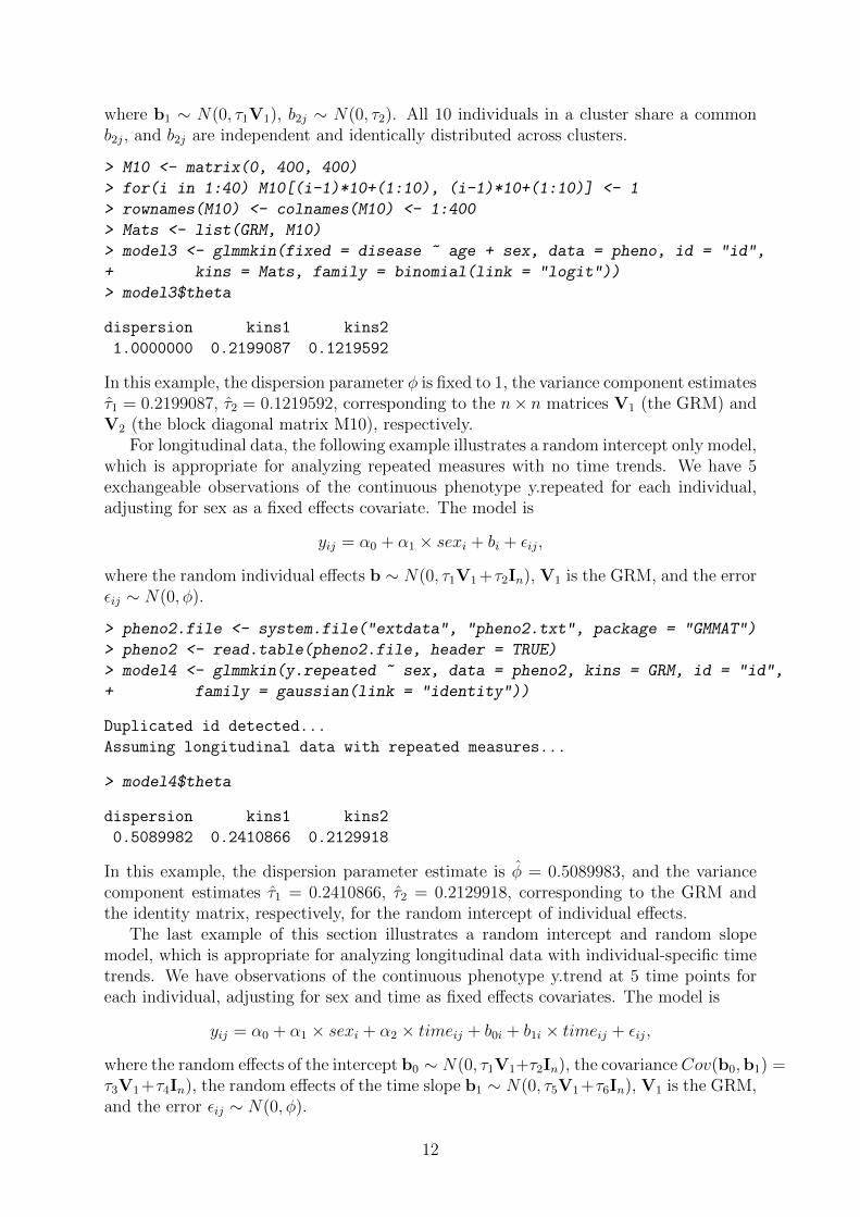
where b1 ∼ N(0, τ1V1), b2j ∼ N(0, τ2). All 10 individuals in a cluster share a commonb2j, and b2j are independent and identically distributed across clusters.
> M10 <- matrix(0, 400, 400)
> for(i in 1:40) M10[(i-1)*10+(1:10), (i-1)*10+(1:10)] <- 1
> rownames(M10) <- colnames(M10) <- 1:400
> Mats <- list(GRM, M10)
> model3 <- glmmkin(fixed = disease ~ age + sex, data = pheno, id = "id",
+ kins = Mats, family = binomial(link = "logit"))
> model3$theta
dispersion kins1 kins2
1.0000000 0.2199087 0.1219592
In this example, the dispersion parameter φ is fixed to 1, the variance component estimatesτ1 = 0.2199087, τ2 = 0.1219592, corresponding to the n× n matrices V1 (the GRM) andV2 (the block diagonal matrix M10), respectively.
For longitudinal data, the following example illustrates a random intercept only model,which is appropriate for analyzing repeated measures with no time trends. We have 5exchangeable observations of the continuous phenotype y.repeated for each individual,adjusting for sex as a fixed effects covariate. The model is
yij = α0 + α1 × sexi + bi + εij,
where the random individual effects b ∼ N(0, τ1V1+τ2In), V1 is the GRM, and the errorεij ∼ N(0, φ).
> pheno2.file <- system.file("extdata", "pheno2.txt", package = "GMMAT")
> pheno2 <- read.table(pheno2.file, header = TRUE)
> model4 <- glmmkin(y.repeated ~ sex, data = pheno2, kins = GRM, id = "id",
+ family = gaussian(link = "identity"))
Duplicated id detected...
Assuming longitudinal data with repeated measures...
> model4$theta
dispersion kins1 kins2
0.5089982 0.2410866 0.2129918
In this example, the dispersion parameter estimate is φ = 0.5089983, and the variancecomponent estimates τ1 = 0.2410866, τ2 = 0.2129918, corresponding to the GRM andthe identity matrix, respectively, for the random intercept of individual effects.
The last example of this section illustrates a random intercept and random slopemodel, which is appropriate for analyzing longitudinal data with individual-specific timetrends. We have observations of the continuous phenotype y.trend at 5 time points foreach individual, adjusting for sex and time as fixed effects covariates. The model is
yij = α0 + α1 × sexi + α2 × timeij + b0i + b1i × timeij + εij,
where the random effects of the intercept b0 ∼ N(0, τ1V1+τ2In), the covariance Cov(b0,b1) =τ3V1+τ4In), the random effects of the time slope b1 ∼ N(0, τ5V1+τ6In), V1 is the GRM,and the error εij ∼ N(0, φ).
12
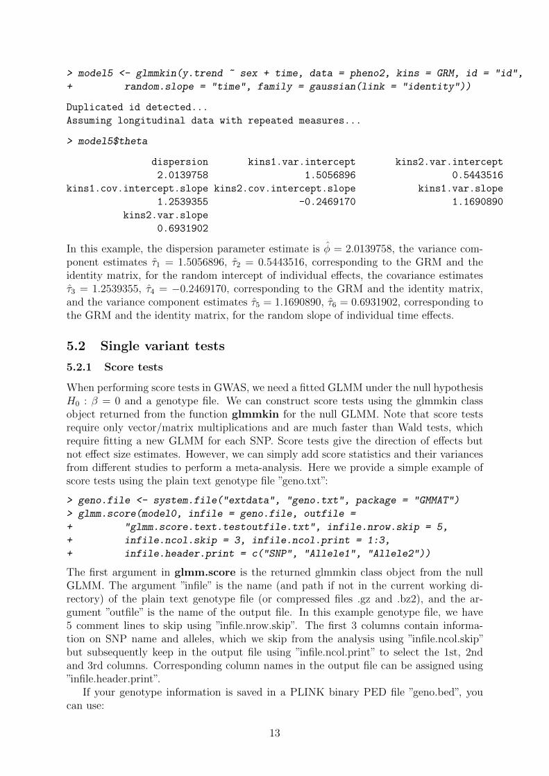
> model5 <- glmmkin(y.trend ~ sex + time, data = pheno2, kins = GRM, id = "id",
+ random.slope = "time", family = gaussian(link = "identity"))
Duplicated id detected...
Assuming longitudinal data with repeated measures...
> model5$theta
dispersion kins1.var.intercept kins2.var.intercept
2.0139758 1.5056896 0.5443516
kins1.cov.intercept.slope kins2.cov.intercept.slope kins1.var.slope
1.2539355 -0.2469170 1.1690890
kins2.var.slope
0.6931902
In this example, the dispersion parameter estimate is φ = 2.0139758, the variance com-ponent estimates τ1 = 1.5056896, τ2 = 0.5443516, corresponding to the GRM and theidentity matrix, for the random intercept of individual effects, the covariance estimatesτ3 = 1.2539355, τ4 = −0.2469170, corresponding to the GRM and the identity matrix,and the variance component estimates τ5 = 1.1690890, τ6 = 0.6931902, corresponding tothe GRM and the identity matrix, for the random slope of individual time effects.
5.2 Single variant tests
5.2.1 Score tests
When performing score tests in GWAS, we need a fitted GLMM under the null hypothesisH0 : β = 0 and a genotype file. We can construct score tests using the glmmkin classobject returned from the function glmmkin for the null GLMM. Note that score testsrequire only vector/matrix multiplications and are much faster than Wald tests, whichrequire fitting a new GLMM for each SNP. Score tests give the direction of effects butnot effect size estimates. However, we can simply add score statistics and their variancesfrom different studies to perform a meta-analysis. Here we provide a simple example ofscore tests using the plain text genotype file ”geno.txt”:
> geno.file <- system.file("extdata", "geno.txt", package = "GMMAT")
> glmm.score(model0, infile = geno.file, outfile =
+ "glmm.score.text.testoutfile.txt", infile.nrow.skip = 5,
+ infile.ncol.skip = 3, infile.ncol.print = 1:3,
+ infile.header.print = c("SNP", "Allele1", "Allele2"))
The first argument in glmm.score is the returned glmmkin class object from the nullGLMM. The argument ”infile” is the name (and path if not in the current working di-rectory) of the plain text genotype file (or compressed files .gz and .bz2), and the ar-gument ”outfile” is the name of the output file. In this example genotype file, we have5 comment lines to skip using ”infile.nrow.skip”. The first 3 columns contain informa-tion on SNP name and alleles, which we skip from the analysis using ”infile.ncol.skip”but subsequently keep in the output file using ”infile.ncol.print” to select the 1st, 2ndand 3rd columns. Corresponding column names in the output file can be assigned using”infile.header.print”.
If your genotype information is saved in a PLINK binary PED file ”geno.bed”, youcan use:
13
> geno.file <- strsplit(system.file("extdata", "geno.bed",
+ package = "GMMAT"), ".bed", fixed = TRUE)[[1]]
> glmm.score(model0, infile = geno.file, outfile =
+ "glmm.score.bed.testoutfile.txt")
Here ”infile” is the prefix (and path if not in the current working directory) of the PLINKfiles (.bed, .bim and .fam). SNP information in the .bim file (in our example, ”geno.bim”)is carried over to the output file.
Alternatively, if your genotype information is saved in a GDS file ”geno.gds”, you canuse:
> geno.file <- system.file("extdata", "geno.gds", package = "GMMAT")
> glmm.score(model0, infile = geno.file, outfile =
+ "glmm.score.gds.testoutfile.txt")
The function glmm.score returns the actual computation time in seconds from itsfunction call for plain text genotype files (or compressed files .gz and .bz2) and PLINKbinary PED files. For GDS genotype files, no value is returned.
5.2.2 Wald tests
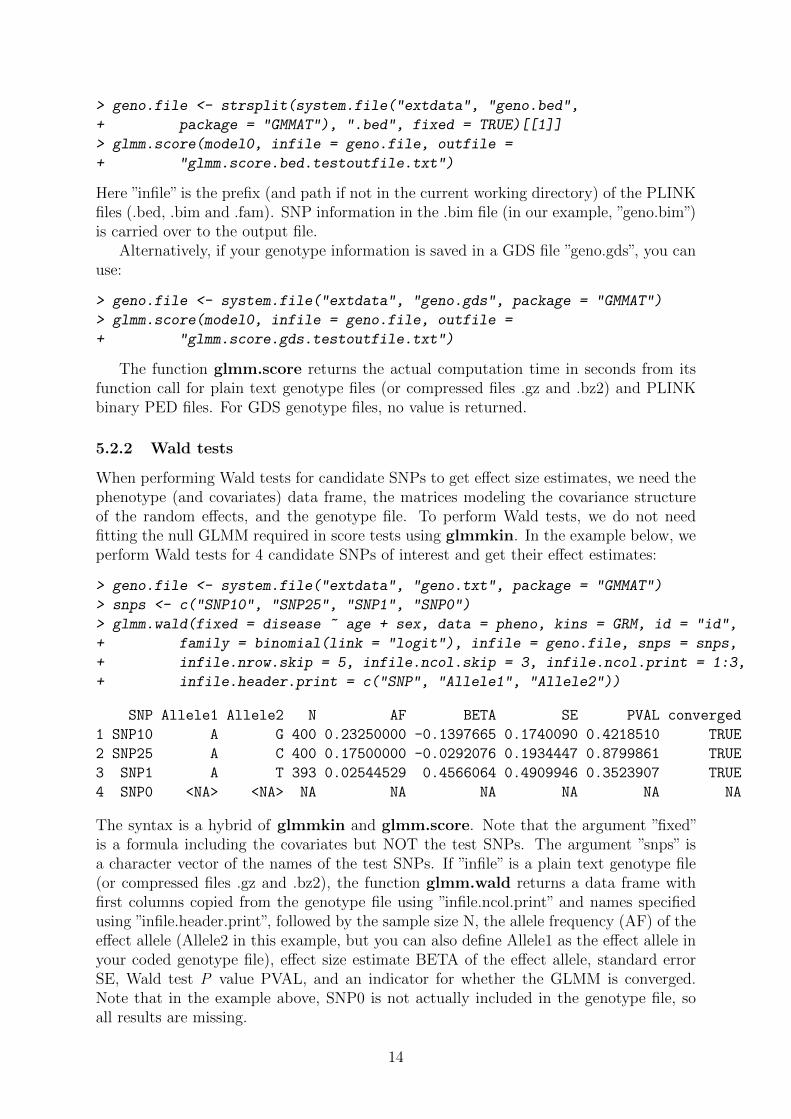
When performing Wald tests for candidate SNPs to get effect size estimates, we need thephenotype (and covariates) data frame, the matrices modeling the covariance structureof the random effects, and the genotype file. To perform Wald tests, we do not needfitting the null GLMM required in score tests using glmmkin. In the example below, weperform Wald tests for 4 candidate SNPs of interest and get their effect estimates:
> geno.file <- system.file("extdata", "geno.txt", package = "GMMAT")
> snps <- c("SNP10", "SNP25", "SNP1", "SNP0")
> glmm.wald(fixed = disease ~ age + sex, data = pheno, kins = GRM, id = "id",
+ family = binomial(link = "logit"), infile = geno.file, snps = snps,
+ infile.nrow.skip = 5, infile.ncol.skip = 3, infile.ncol.print = 1:3,
+ infile.header.print = c("SNP", "Allele1", "Allele2"))
SNP Allele1 Allele2 N AF BETA SE PVAL converged
1 SNP10 A G 400 0.23250000 -0.1397665 0.1740090 0.4218510 TRUE
2 SNP25 A C 400 0.17500000 -0.0292076 0.1934447 0.8799861 TRUE
3 SNP1 A T 393 0.02544529 0.4566064 0.4909946 0.3523907 TRUE
4 SNP0 <NA> <NA> NA NA NA NA NA NA
The syntax is a hybrid of glmmkin and glmm.score. Note that the argument ”fixed”is a formula including the covariates but NOT the test SNPs. The argument ”snps” isa character vector of the names of the test SNPs. If ”infile” is a plain text genotype file(or compressed files .gz and .bz2), the function glmm.wald returns a data frame withfirst columns copied from the genotype file using ”infile.ncol.print” and names specifiedusing ”infile.header.print”, followed by the sample size N, the allele frequency (AF) of theeffect allele (Allele2 in this example, but you can also define Allele1 as the effect allele inyour coded genotype file), effect size estimate BETA of the effect allele, standard errorSE, Wald test P value PVAL, and an indicator for whether the GLMM is converged.Note that in the example above, SNP0 is not actually included in the genotype file, soall results are missing.
14
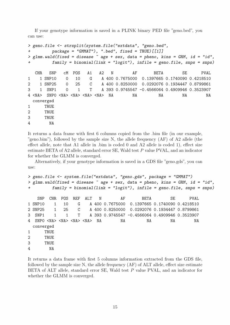
If your genotype information is saved in a PLINK binary PED file ”geno.bed”, youcan use:
> geno.file <- strsplit(system.file("extdata", "geno.bed",
+ package = "GMMAT"), ".bed", fixed = TRUE)[[1]]
> glmm.wald(fixed = disease ~ age + sex, data = pheno, kins = GRM, id = "id",
+ family = binomial(link = "logit"), infile = geno.file, snps = snps)
CHR SNP cM POS A1 A2 N AF BETA SE PVAL
1 1 SNP10 0 10 G A 400 0.7675000 0.1397665 0.1740090 0.4218510
2 1 SNP25 0 25 C A 400 0.8250000 0.0292076 0.1934447 0.8799861
3 1 SNP1 0 1 T A 393 0.9745547 -0.4566064 0.4909946 0.3523907
4 <NA> SNP0 <NA> <NA> <NA> <NA> NA NA NA NA NA
converged
1 TRUE
2 TRUE
3 TRUE
4 NA
It returns a data frame with first 6 columns copied from the .bim file (in our example,”geno.bim”), followed by the sample size N, the allele frequency (AF) of A2 allele (theeffect allele, note that A1 allele in .bim is coded 0 and A2 allele is coded 1), effect sizeestimate BETA of A2 allele, standard error SE, Wald test P value PVAL, and an indicatorfor whether the GLMM is converged.
Alternatively, if your genotype information is saved in a GDS file ”geno.gds”, you canuse:
> geno.file <- system.file("extdata", "geno.gds", package = "GMMAT")
> glmm.wald(fixed = disease ~ age + sex, data = pheno, kins = GRM, id = "id",
+ family = binomial(link = "logit"), infile = geno.file, snps = snps)
SNP CHR POS REF ALT N AF BETA SE PVAL
1 SNP10 1 10 G A 400 0.7675000 0.1397665 0.1740090 0.4218510
2 SNP25 1 25 C A 400 0.8250000 0.0292076 0.1934447 0.8799861
3 SNP1 1 1 T A 393 0.9745547 -0.4566064 0.4909946 0.3523907
4 SNP0 <NA> <NA> <NA> <NA> NA NA NA NA NA
converged
1 TRUE
2 TRUE
3 TRUE
4 NA
It returns a data frame with first 5 columns information extracted from the GDS file,followed by the sample size N, the allele frequency (AF) of ALT allele, effect size estimateBETA of ALT allele, standard error SE, Wald test P value PVAL, and an indicator forwhether the GLMM is converged.
15
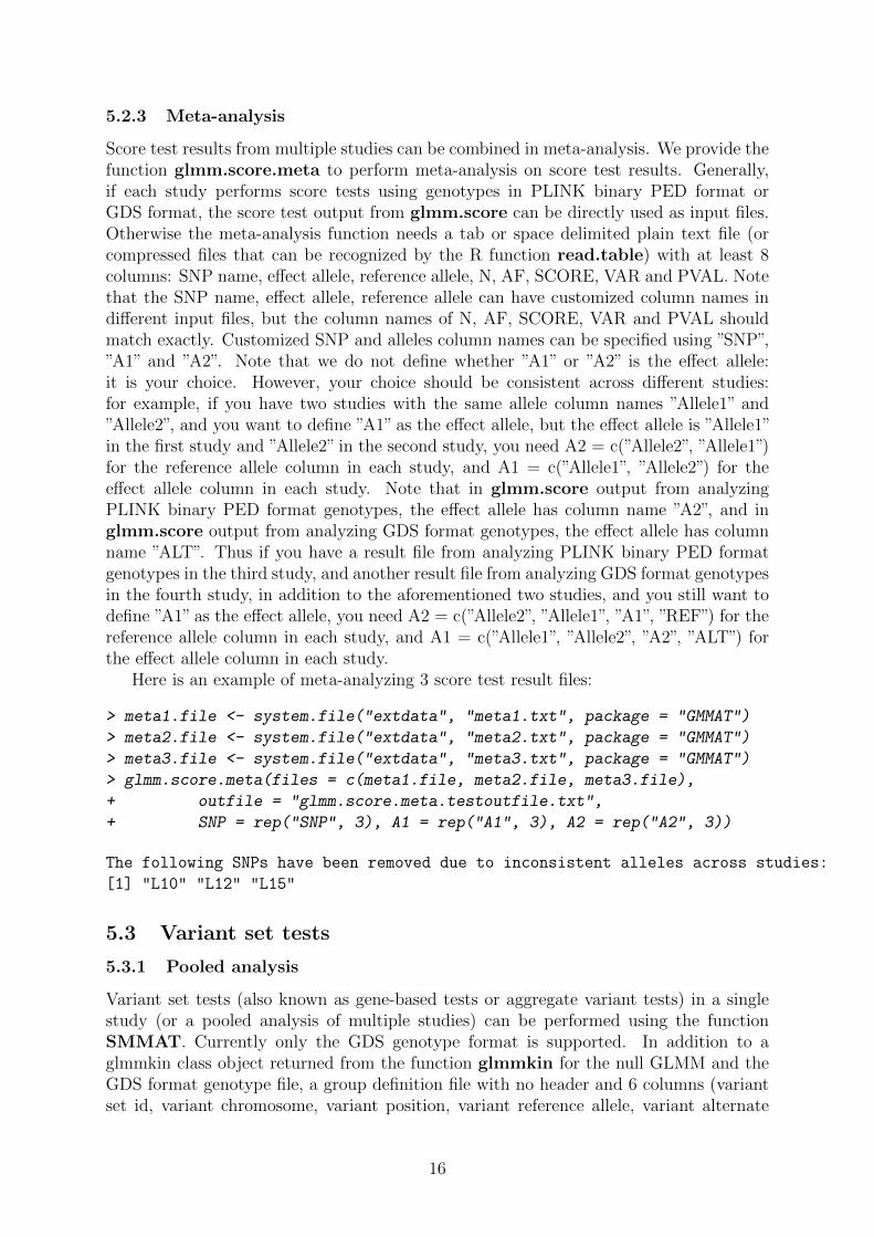
5.2.3 Meta-analysis
Score test results from multiple studies can be combined in meta-analysis. We provide thefunction glmm.score.meta to perform meta-analysis on score test results. Generally,if each study performs score tests using genotypes in PLINK binary PED format orGDS format, the score test output from glmm.score can be directly used as input files.Otherwise the meta-analysis function needs a tab or space delimited plain text file (orcompressed files that can be recognized by the R function read.table) with at least 8columns: SNP name, effect allele, reference allele, N, AF, SCORE, VAR and PVAL. Notethat the SNP name, effect allele, reference allele can have customized column names indifferent input files, but the column names of N, AF, SCORE, VAR and PVAL shouldmatch exactly. Customized SNP and alleles column names can be specified using ”SNP”,”A1” and ”A2”. Note that we do not define whether ”A1” or ”A2” is the effect allele:it is your choice. However, your choice should be consistent across different studies:for example, if you have two studies with the same allele column names ”Allele1” and”Allele2”, and you want to define ”A1” as the effect allele, but the effect allele is ”Allele1”in the first study and ”Allele2” in the second study, you need A2 = c(”Allele2”, ”Allele1”)for the reference allele column in each study, and A1 = c(”Allele1”, ”Allele2”) for theeffect allele column in each study. Note that in glmm.score output from analyzingPLINK binary PED format genotypes, the effect allele has column name ”A2”, and inglmm.score output from analyzing GDS format genotypes, the effect allele has columnname ”ALT”. Thus if you have a result file from analyzing PLINK binary PED formatgenotypes in the third study, and another result file from analyzing GDS format genotypesin the fourth study, in addition to the aforementioned two studies, and you still want todefine ”A1” as the effect allele, you need A2 = c(”Allele2”, ”Allele1”, ”A1”, ”REF”) for thereference allele column in each study, and A1 = c(”Allele1”, ”Allele2”, ”A2”, ”ALT”) forthe effect allele column in each study.
Here is an example of meta-analyzing 3 score test result files:
> meta1.file <- system.file("extdata", "meta1.txt", package = "GMMAT")
> meta2.file <- system.file("extdata", "meta2.txt", package = "GMMAT")
> meta3.file <- system.file("extdata", "meta3.txt", package = "GMMAT")
> glmm.score.meta(files = c(meta1.file, meta2.file, meta3.file),
+ outfile = "glmm.score.meta.testoutfile.txt",
+ SNP = rep("SNP", 3), A1 = rep("A1", 3), A2 = rep("A2", 3))
The following SNPs have been removed due to inconsistent alleles across studies:
[1] "L10" "L12" "L15"
5.3 Variant set tests
5.3.1 Pooled analysis
Variant set tests (also known as gene-based tests or aggregate variant tests) in a singlestudy (or a pooled analysis of multiple studies) can be performed using the functionSMMAT. Currently only the GDS genotype format is supported. In addition to aglmmkin class object returned from the function glmmkin for the null GLMM and theGDS format genotype file, a group definition file with no header and 6 columns (variantset id, variant chromosome, variant position, variant reference allele, variant alternate
16
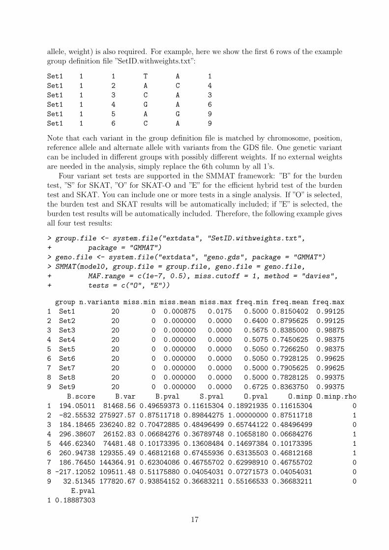
allele, weight) is also required. For example, here we show the first 6 rows of the examplegroup definition file ”SetID.withweights.txt”:
Set1 1 1 T A 1
Set1 1 2 A C 4
Set1 1 3 C A 3
Set1 1 4 G A 6
Set1 1 5 A G 9
Set1 1 6 C A 9
Note that each variant in the group definition file is matched by chromosome, position,reference allele and alternate allele with variants from the GDS file. One genetic variantcan be included in different groups with possibly different weights. If no external weightsare needed in the analysis, simply replace the 6th column by all 1’s.
Four variant set tests are supported in the SMMAT framework: ”B” for the burdentest, ”S” for SKAT, ”O” for SKAT-O and ”E” for the efficient hybrid test of the burdentest and SKAT. You can include one or more tests in a single analysis. If ”O” is selected,the burden test and SKAT results will be automatically included; if ”E” is selected, theburden test results will be automatically included. Therefore, the following example givesall four test results:
> group.file <- system.file("extdata", "SetID.withweights.txt",
+ package = "GMMAT")
> geno.file <- system.file("extdata", "geno.gds", package = "GMMAT")
> SMMAT(model0, group.file = group.file, geno.file = geno.file,
+ MAF.range = c(1e-7, 0.5), miss.cutoff = 1, method = "davies",
+ tests = c("O", "E"))
group n.variants miss.min miss.mean miss.max freq.min freq.mean freq.max
1 Set1 20 0 0.000875 0.0175 0.5000 0.8150402 0.99125
2 Set2 20 0 0.000000 0.0000 0.6400 0.8795625 0.99125
3 Set3 20 0 0.000000 0.0000 0.5675 0.8385000 0.98875
4 Set4 20 0 0.000000 0.0000 0.5075 0.7450625 0.98375
5 Set5 20 0 0.000000 0.0000 0.5050 0.7266250 0.98375
6 Set6 20 0 0.000000 0.0000 0.5050 0.7928125 0.99625
7 Set7 20 0 0.000000 0.0000 0.5000 0.7905625 0.99625
8 Set8 20 0 0.000000 0.0000 0.5000 0.7828125 0.99375
9 Set9 20 0 0.000000 0.0000 0.6725 0.8363750 0.99375
B.score B.var B.pval S.pval O.pval O.minp O.minp.rho
1 194.05011 81468.56 0.49659373 0.11615304 0.18921935 0.11615304 0
2 -82.55532 275927.57 0.87511718 0.89844275 1.00000000 0.87511718 1
3 184.18465 236240.82 0.70472885 0.48496499 0.65744122 0.48496499 0
4 296.38607 26152.83 0.06684276 0.36789748 0.10658180 0.06684276 1
5 446.62340 74481.48 0.10173395 0.13608484 0.14697384 0.10173395 1
6 260.94738 129355.49 0.46812168 0.67455936 0.63135503 0.46812168 1
7 186.76450 144364.91 0.62304086 0.46755702 0.62998910 0.46755702 0
8 -217.12052 109511.48 0.51175880 0.04054031 0.07271573 0.04054031 0
9 32.51345 177820.67 0.93854152 0.36683211 0.55166533 0.36683211 0
E.pval
1 0.18887303
17
2 0.96115053
3 0.50543498
4 0.11280647
5 0.30955819
6 0.57325090
7 0.56439536
8 0.05185727
9 0.59186822
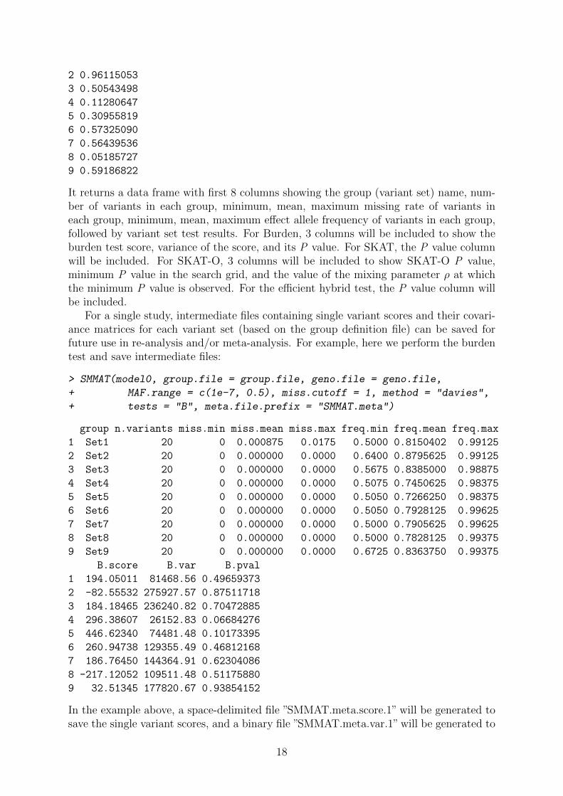
It returns a data frame with first 8 columns showing the group (variant set) name, num-ber of variants in each group, minimum, mean, maximum missing rate of variants ineach group, minimum, mean, maximum effect allele frequency of variants in each group,followed by variant set test results. For Burden, 3 columns will be included to show theburden test score, variance of the score, and its P value. For SKAT, the P value columnwill be included. For SKAT-O, 3 columns will be included to show SKAT-O P value,minimum P value in the search grid, and the value of the mixing parameter ρ at whichthe minimum P value is observed. For the efficient hybrid test, the P value column willbe included.
For a single study, intermediate files containing single variant scores and their covari-ance matrices for each variant set (based on the group definition file) can be saved forfuture use in re-analysis and/or meta-analysis. For example, here we perform the burdentest and save intermediate files:
> SMMAT(model0, group.file = group.file, geno.file = geno.file,
+ MAF.range = c(1e-7, 0.5), miss.cutoff = 1, method = "davies",
+ tests = "B", meta.file.prefix = "SMMAT.meta")
group n.variants miss.min miss.mean miss.max freq.min freq.mean freq.max
1 Set1 20 0 0.000875 0.0175 0.5000 0.8150402 0.99125
2 Set2 20 0 0.000000 0.0000 0.6400 0.8795625 0.99125
3 Set3 20 0 0.000000 0.0000 0.5675 0.8385000 0.98875
4 Set4 20 0 0.000000 0.0000 0.5075 0.7450625 0.98375
5 Set5 20 0 0.000000 0.0000 0.5050 0.7266250 0.98375
6 Set6 20 0 0.000000 0.0000 0.5050 0.7928125 0.99625
7 Set7 20 0 0.000000 0.0000 0.5000 0.7905625 0.99625
8 Set8 20 0 0.000000 0.0000 0.5000 0.7828125 0.99375
9 Set9 20 0 0.000000 0.0000 0.6725 0.8363750 0.99375
B.score B.var B.pval
1 194.05011 81468.56 0.49659373
2 -82.55532 275927.57 0.87511718
3 184.18465 236240.82 0.70472885
4 296.38607 26152.83 0.06684276
5 446.62340 74481.48 0.10173395
6 260.94738 129355.49 0.46812168
7 186.76450 144364.91 0.62304086
8 -217.12052 109511.48 0.51175880
9 32.51345 177820.67 0.93854152
In the example above, a space-delimited file ”SMMAT.meta.score.1” will be generated tosave the single variant scores, and a binary file ”SMMAT.meta.var.1” will be generated to
18
save the covariance matrices for the variant sets. Note that the binary file is not human-readable, but can be used by SMMAT.meta in re-analysis and/or meta-analysis.
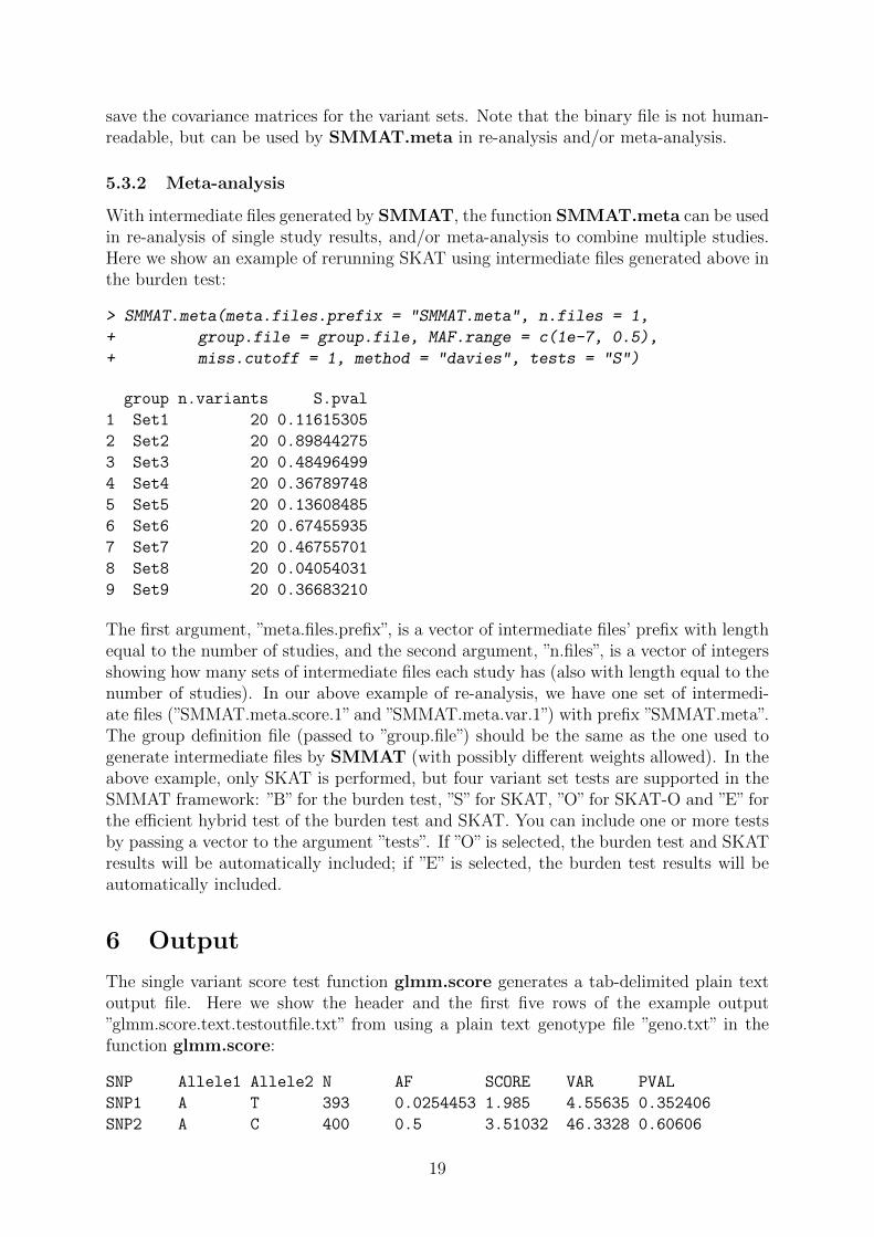
5.3.2 Meta-analysis
With intermediate files generated by SMMAT, the function SMMAT.meta can be usedin re-analysis of single study results, and/or meta-analysis to combine multiple studies.Here we show an example of rerunning SKAT using intermediate files generated above inthe burden test:
> SMMAT.meta(meta.files.prefix = "SMMAT.meta", n.files = 1,
+ group.file = group.file, MAF.range = c(1e-7, 0.5),
+ miss.cutoff = 1, method = "davies", tests = "S")
group n.variants S.pval
1 Set1 20 0.11615305
2 Set2 20 0.89844275
3 Set3 20 0.48496499
4 Set4 20 0.36789748
5 Set5 20 0.13608485
6 Set6 20 0.67455935
7 Set7 20 0.46755701
8 Set8 20 0.04054031
9 Set9 20 0.36683210
The first argument, ”meta.files.prefix”, is a vector of intermediate files’ prefix with lengthequal to the number of studies, and the second argument, ”n.files”, is a vector of integersshowing how many sets of intermediate files each study has (also with length equal to thenumber of studies). In our above example of re-analysis, we have one set of intermedi-ate files (”SMMAT.meta.score.1” and ”SMMAT.meta.var.1”) with prefix ”SMMAT.meta”.The group definition file (passed to ”group.file”) should be the same as the one used togenerate intermediate files by SMMAT (with possibly different weights allowed). In theabove example, only SKAT is performed, but four variant set tests are supported in theSMMAT framework: ”B” for the burden test, ”S” for SKAT, ”O” for SKAT-O and ”E” forthe efficient hybrid test of the burden test and SKAT. You can include one or more testsby passing a vector to the argument ”tests”. If ”O” is selected, the burden test and SKATresults will be automatically included; if ”E” is selected, the burden test results will beautomatically included.
6 Output
The single variant score test function glmm.score generates a tab-delimited plain textoutput file. Here we show the header and the first five rows of the example output”glmm.score.text.testoutfile.txt” from using a plain text genotype file ”geno.txt” in thefunction glmm.score:
SNP Allele1 Allele2 N AF SCORE VAR PVAL
SNP1 A T 393 0.0254453 1.985 4.55635 0.352406
SNP2 A C 400 0.5 3.51032 46.3328 0.60606
19
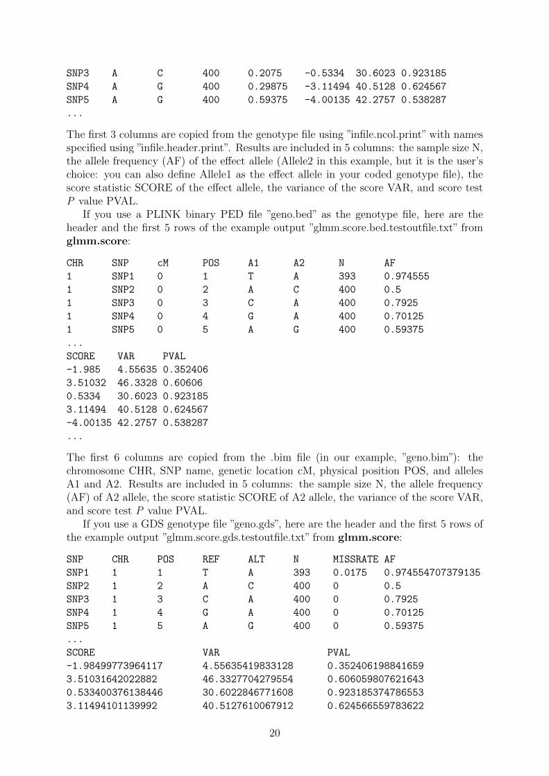
SNP3 A C 400 0.2075 -0.5334 30.6023 0.923185
SNP4 A G 400 0.29875 -3.11494 40.5128 0.624567
SNP5 A G 400 0.59375 -4.00135 42.2757 0.538287
...
The first 3 columns are copied from the genotype file using ”infile.ncol.print” with namesspecified using ”infile.header.print”. Results are included in 5 columns: the sample size N,the allele frequency (AF) of the effect allele (Allele2 in this example, but it is the user’schoice: you can also define Allele1 as the effect allele in your coded genotype file), thescore statistic SCORE of the effect allele, the variance of the score VAR, and score testP value PVAL.
If you use a PLINK binary PED file ”geno.bed” as the genotype file, here are theheader and the first 5 rows of the example output ”glmm.score.bed.testoutfile.txt” fromglmm.score:
CHR SNP cM POS A1 A2 N AF
1 SNP1 0 1 T A 393 0.974555
1 SNP2 0 2 A C 400 0.5
1 SNP3 0 3 C A 400 0.7925
1 SNP4 0 4 G A 400 0.70125
1 SNP5 0 5 A G 400 0.59375
...
SCORE VAR PVAL
-1.985 4.55635 0.352406
3.51032 46.3328 0.60606
0.5334 30.6023 0.923185
3.11494 40.5128 0.624567
-4.00135 42.2757 0.538287
...
The first 6 columns are copied from the .bim file (in our example, ”geno.bim”): thechromosome CHR, SNP name, genetic location cM, physical position POS, and allelesA1 and A2. Results are included in 5 columns: the sample size N, the allele frequency(AF) of A2 allele, the score statistic SCORE of A2 allele, the variance of the score VAR,and score test P value PVAL.
If you use a GDS genotype file ”geno.gds”, here are the header and the first 5 rows ofthe example output ”glmm.score.gds.testoutfile.txt” from glmm.score:
SNP CHR POS REF ALT N MISSRATE AF
SNP1 1 1 T A 393 0.0175 0.974554707379135
SNP2 1 2 A C 400 0 0.5
SNP3 1 3 C A 400 0 0.7925
SNP4 1 4 G A 400 0 0.70125
SNP5 1 5 A G 400 0 0.59375
...
SCORE VAR PVAL
-1.98499773964117 4.55635419833128 0.352406198841659
3.51031642022882 46.3327704279554 0.606059807621643
0.533400376138446 30.6022846771608 0.923185374786553
3.11494101139992 40.5127610067912 0.624566559783622
20
-4.00135050079485 42.2757210650549 0.538287231263494
...
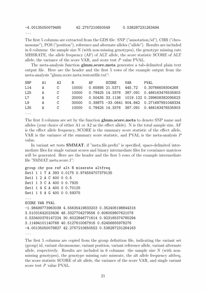
The first 5 columns are extracted from the GDS file: SNP (”annotation/id”), CHR (”chro-mosome”), POS (”position”), reference and alternate alleles (”allele”). Results are includedin 6 columns: the sample size N (with non-missing genotypes), the genotype missing rateMISSRATE, the allele frequency (AF) of ALT allele, the score statistic SCORE of ALTallele, the variance of the score VAR, and score test P value PVAL.
The meta-analysis function glmm.score.meta generates a tab-delimited plain textoutput file. Here are the header and the first 5 rows of the example output from themeta-analysis ”glmm.score.meta.testoutfile.txt”:
SNP A1 A2 N AF SCORE VAR PVAL
L14 A C 10000 0.65895 21.5371 445.72 0.30766609304268
L25 A C 10000 0.78425 14.3376 387.091 0.466163476535903
L7 A C 20000 0.50435 33.1136 1019.122 0.299608382095623
L9 A C 30000 0.39875 -33.0641 904.842 0.271687891048334
L35 A C 10000 0.78425 14.3376 387.091 0.466163476535903
...
The first 3 columns are set by the function glmm.score.meta to denote SNP name andalleles (your choice of either A1 or A2 as the effect allele). N is the total sample size, AFis the effect allele frequency, SCORE is the summary score statistic of the effect allele,VAR is the variance of the summary score statistic, and PVAL is the meta-analysis Pvalue.
In variant set tests SMMAT, if ”meta.file.prefix” is specified, space-delimited inter-mediate files for single variant scores and binary intermediate files for covariance matriceswill be generated. Here are the header and the first 5 rows of the example intermediatefile ”SMMAT.meta.score.1”:
group chr pos ref alt N missrate altfreq
Set1 1 1 T A 393 0.0175 0.974554707379135
Set1 1 2 A C 400 0 0.5
Set1 1 3 C A 400 0 0.7925
Set1 1 4 G A 400 0 0.70125
Set1 1 5 A G 400 0 0.59375
...
SCORE VAR PVAL
-1.98499773963038 4.55635419833203 0.352406198844316
3.51031642023436 46.3327704279556 0.606059807621076
0.533400376147224 30.6022846771614 0.923185374785294
3.11494101140768 40.5127610067916 0.62456655978276
-4.00135050078827 42.2757210650552 0.538287231264163
...
The first 5 columns are copied from the group definition file, indicating the variant set(group) id, variant chromosome, variant position, variant reference allele, variant alternateallele, respectively. Results are included in 6 columns: the sample size N (with non-missing genotypes), the genotype missing rate missrate, the alt allele frequency altfreq,the score statistic SCORE of alt allele, the variance of the score VAR, and single variantscore test P value PVAL.
21

7 Advanced options
7.1 Alternative model fitting algorithms
By default we use the Average Information REML algorithm13,14 to fit the GLMM inglmmkin, which is computationally efficient and recommended in most cases. However,there are also alternative model fitting algorithms:
method = "REML", method.optim = "Brent"
It maximizes the restricted likelihood using the derivative-free Brent method,15 but onlyworks when there is one matrix for the covariance structure of the random effects.
method = "ML", method.optim = "Brent"
It maximizes the likelihood using the Brent method.
method = "REML", method.optim = "Nelder-Mead"
It maximizes the restricted likelihood using the Nelder-Mead method,16 however it isusually very slow in large samples.
method = "ML", method.optim = "Nelder-Mead"
It maximizes the likelihood using the Nelder-Mead method.Note that the default algorithm is
method = "REML", method.optim = "AI"
A maximum likelihood version of Average Information algorithm is not available inglmmkin.
7.2 Changing model fitting parameters
By default we set the maximum number of iteration to 500 and tolerance to declareconvergence to 1e-5:
maxiter = 500, tol = 1e-5
These parameters can be changed. When using the Brent method for maximizing thelikelihood (or restricted likelihood), we specify the search range of the ratio of the variancecomponent parameter τ1 over the dispersion parameter φ to be between 1e-5 and 1e5,and we divide the search region evenly into 10 regions on the log scale:
taumin = 1e-5, taumax = 1e5, tauregion = 10
These parameters can also be changed, but they are only effective when using the Brentmethod.
22
7.3 Missing genotypes
It is recommended to perform genotype quality control prior to analysis to impute missinggenotypes or filter out SNPs with high missing rates. However, GMMAT does allow miss-ing genotypes, and imputes to the mean value by default. Alternatively, in glmm.scoreand glmm.wald, missing genotypes can be omitted from the analysis using
missing.method = "omit"
In variant set tests using SMMAT, instead of imputing missing genotypes to the meanvalue, you can impute missing genotypes to 0 (homozygous reference allele) using
missing.method = "impute2zero"
If using a plain text (or compressed .gz and .bz2) genotype file, missing genotypesshould be coded as ”NA”. If you have missing genotypes coded in a different way, youcan specify this in the argument ”infile.na”.
7.4 Reordered genotypes
The genotype file (either a plain text file, a PLINK binary PED file, or a GDS file) caninclude more individuals than in the phenotype and covariates data frame, and they canbe in different orders. GMMAT handles this issue using an argument ”select” in bothglmm.score and glmm.wald. For example, if the order of individuals in your genotypefile is A, B, C, D, but you only have 3 unique individuals (with order C, A, B) in thefitted ”obj” (for glmm.score) or in the data frame ”data” (for glmm.wald), then youcan specify
select = c(2, 3, 1, 0)
to reflect the order of individuals. Note that since individual D is not included, its orderis assigned to 0. The length of the vector must match the number of individuals in yourgenotype file. Also note that if there are observations with missing phenotype/covariatesin ”data”, ”select” for glmm.wald should match to ”data” before removing any missingvalues, while ”select” for glmm.score should match to ”obj” (in which missing valueshave been excluded).
In variant set tests, SMMAT will extract ID from ”null.obj” using ”id include” re-turned in the glmmkin fitted null model object. The ID will be matched to ”sample.id”in the GDS genotype file.
7.5 Parallel computing
Parallel computing can be enabled in glmm.score and SMMAT using the argument”ncores”to specify how many cores you would like to use on a computing node. By default”ncores” is 1, meaning that these functions will run in a single thread. Currently parallelcomputing is only implemented for GDS format genotype files.
If you enable parallel computing and save intermediate files, you will get multi-ple sets of intermediate files. For example, if your ”ncores” is 12 and you specified”meta.file.prefix” to ”study1”, then you will get 12 sets of (totaling 24) intermediate files”study1.score.1”, ”study1.var.1”, ”study1.score.2”, ”study1.var.2”, ..., ”study1.score.12”,”study1.var.12”. Later in the meta-analysis to combine with 2 sets of intermediate files”study2.score.1”, ”study2.var.1”, ”study2.score.2”, ”study2.var.2”, you will need to use
23
meta.files.prefix = c("study1", "study2"), n.files = c(12, 2)
If your R is configured with Intel MKL and you would like to enable parallel comput-ing, it is recommended that you set the environmental variable ”MKL NUM THREADS”to 1 before running R to avoid hanging. Alternatively, you can do this at the beginningof your R script by using
> Sys.setenv(MKL_NUM_THREADS = 1)
7.6 Variant filters
Variants can be filtered in glmm.score and SMMAT based on minor allele frequency(MAF) and missing rate filters. The argument ”MAF.range” specifies the minimum andmaximum MAFs for a variant to be included in the analysis. By default the minimumMAF is 1×10⁻⁷ and the maximum MAF is 0.5, meaning that only monomorphic markersin the sample will be excluded (if your sample size is no more than 5 million). Theargument ”miss.cutoff” specifies the maximum missing rate for a variant to be includedin the analysis. By default it is set to 1, meaning that no variants will be removed dueto high genotype missing rates.
7.7 Internal minor allele frequency weights
Internal weights are calculated based on the minor allele frequency (NOT the effect allelefrequency, therefore, variants with effect allele frequencies 0.01 and 0.99 have the sameweights) as a beta probability density function. Internal weights are multiplied by theexternal weights given in the last column of the group definition file. To turn off internalweights, use
MAF.weights.beta = c(1, 1)
to assign flat weights, as a beta distribution with parameters 1 and 1 is a uniform distri-bution on the interval between 0 and 1.
7.8 Allele flipping
In variant set tests SMMAT, by default the alt allele is used as the coding allele andvariants in each variant set are matched strictly on chromosome, position, reference andalternate alleles.
The argument ”auto.flip” allows automatic allele flipping if a specified variant is notfound in the genotype file, but a variant at the same chromosome and position withreference allele matching the alternate allele in the group definition file ”group.file”, andalternate allele matching the reference allele in the group definition file ”group.file”, tobe included in the analysis. Please use with caution for whole genome sequence data, asboth ref/alt and alt/ref variants at the same position are not uncommon, and they arelikely two different variants, rather than allele flipping.
The argument ”use.minor.allele” allows using the minor allele instead of the alt alleleas the coding allele in variant set tests. Note that this choice does not change ”S” forSKAT results, but ”B” for the burden test, ”O” for SKAT-O and ”E” for efficient hybridtest of the burden test and SKAT results will be affected. Generally the alt allele caneither be the minor or the major allele. If in a variant set, different variants with alt allele
24
frequencies 0.001 and 0.998 are combined together in a burden test, the results would bedifficult to interpret. We generally recommend turning on the ”use.minor.allele” option,unless you know the ancestry alleles explicitly and the specific scientific hypothesis clearlythat you would like to test. Along with the MAF filter, this option is useful for combiningrare mutations, assuming rare allele effects are in the same direction.
7.9 P values of weighted sum of chi-squares
In variant set tests SMMAT, you can use 3 methods in the ”method” argument tocompute P values of weighted sum of chi-square distributions: ”davies”,17 ”kuonen”18 and”liu”.19 By default ”davies” is used, if it returns an error message in the calculation, or aP value greater than 1, or less than 1× 10⁻⁵, ”kuonen” method will be used. If ”kuonen”method fails to compute the P value, ”liu” method will be used.
7.10 Heterogeneous genetic effects in variant set meta-analysis
Heterogeneous genetic effects20 are allowed in variant set tests meta-analysis functionSMMAT.meta, by specifying groups using the ”cohort.group.idx”argument. By defaultall studies are assumed to share the same genetic effects in the meta-analysis, and thiscan be changed by assigning different group indices to studies. For example,
cohort.group.idx = c("a","b","a","a","b")
means cohorts 1, 3, 4 are assumed to have homogeneous genetic effects, and cohorts 2, 5are in another group with homogeneous genetic effects (but possibly heterogeneous withgroup ”a”).
7.11 Other options
By default, genotypes are centered to the mean before the analysis in single variant tests.You can turn this feature off by specifying
center = FALSE
in both glmm.score and glmm.wald functions to use raw genotypes.If your genotype file is a plain text (or a compressed .gz and .bz2 file), and you want to
read in fewer lines than all lines included in the file, you can use the ”infile.nrow”argumentto specify how many lines (including lines to be skipped using ”infile.nrow.skip”) you wantto read in. By default the delimiter is assumed to be a tab, but you can change it using the”infile.sep” argument. These options are implemented in glmm.score and glmm.wald.
In the score test function glmm.score, by default 100 SNPs are tested in a batch. Youcan change it using the ”nperbatch” argument, but the computational time can increasesubstantially if it is either too small or too large, depending on the performance of yourcomputing system.
If you perform Wald tests glmm.wald and use a plain text (or a compressed .gzand .bz2) file, and your SNPs are not in your first column, you can change ”snp.col” inglmm.wald to indicate which column is your SNP name.
In the variant set tests SMMAT, by default the group definition file ”group.file”should be tab delimited, but you can change it using the ”group.file.sep” argument. Alsothere is a ”Garbage.Collection” argument (default FALSE), if turned on, SMMAT will
25
call the function gc for each variant set tested. It helps save memory footprint, but thecomputation speed might be slower.
8 Version
8.1 Version 0.6 (October 12, 2015)
Initial public release of GMMAT.
8.2 Version 0.7 (January 22, 2016)
1. Merged old functions glmm.score.text and glmm.score.bed to glmm.score.
2. Merged old functions glmm.wald.text and glmm.wald.bed to glmm.wald.
3. glmm.score now takes ”obj”, a glmmkin class object returned from glmmkin toset up the score test, instead of ”res” and ”P” from old functions glmm.score.textand glmm.score.bed.
4. Implemented model fitting with fixed variance components in glmmkin, and modelrefitting when variance component estimates are on the boundary of the parameterspace, and default unconverged Average Information REML to derivative-free Brentmethod (one variance component parameter) or Nelder-Mead method (more thanone variance component parameters).
5. Implemented offset in glmmkin.
6. Renamed alpha, eta, mu to coefficients, linear.predictors, fitted.values in glmmkinreturned object.
7. Implemented score test meta-analysis function glmm.score.meta.
8. Fixed minor bugs in glmm.wald to handle errors in fitting each alternative GLMM,and minor bugs in fitting alternative GLMMs using derivative-free algorithms.
8.3 Version 0.7-1 (January 22, 2016)
Light version of v0.7: same features as v0.7 except that this light version does not dependon the C++ library boost and cannot take compressed plain text files .gz and .bz2 asgenotype files.
8.4 Version 0.9 (March 9, 2018)
1. Added ”id include” to glmmkin returned object to indicate which rows in the datahave nonmissing outcome/covariates and are included in the model fit, which isuseful to create
> select <- match(geno_ID, pheno_ID[obj$id_include])
> select[is.na(select)] <- 0
that can be used as the ”select” argument in glmm.score.
26
2. Removed memory duplicates for big matrices in C++ and R code.
3. Support for GDS format genotype files implemented in functions glmm.score andglmm.wald, with optional parallel computing.
4. MAF.range and miss.cutoff implemented in glmm.score for minor allele frequencyand missing rate filters.
5. Implemented variant set tests glmm.rvtests, including burden test, SKAT, SKAT-O and SMMAT, with optional parallel computing.
6. Implemented variant set re-analysis/meta-analysis function glmm.rvtests.meta.
7. Implemented heteroscedastic linear mixed models in glmmkin and glmm.wald byspecifying ”groups”.
8.5 Version 0.9.1 (May 13, 2018)
1. In variant set tests glmm.rvtests and glmm.rvtests.meta, tests ”Burden”, ”SKAT”,”SKAT-O” and ”SMMAT” changed to ”B”, ”S”, ”O” and ”E”, respectively, to denote4 variant set tests in the SMMAT framework: the burden test, SKAT, SKAT-Oand the efficient hybrid test of the burden test and SKAT.
2. Implemented known weights (e.g. binomial denominator) in glmmkin and glmm.waldby passing the argument ”weights” to the glm object ”fixed”
3. Implemented internal MAF-based weights, using the argument ”MAF.weights.beta”to denote the two beta probability density function parameters. Note that theweights are calculated on the minor allele frequency (not the effect allele frequency).Internal weights are multiplied by the external weights given in the last column ofthe group definition file.
8.6 Version 0.9.2 (June 8, 2018)
1. In variant set tests glmm.rvtests and glmm.rvtests.meta, test ”O” (SKAT-Oin the SMMAT framework) p-value switched to minimum p-value multipled by thenumber of points on the search grid if the integration result is larger than the latter(consistent with implementation in the SKAT package).
8.7 Version 0.9.3 (July 18, 2018)
1. In the null model fitting function glmmkin, prior weights (e.g. binomial denomi-nators for binomial distributions) coerced to a vector.
2. In the null model fitting function glmmkin, model matrix X for fixed effects nowincluded in the returned object.
27
8.8 Version 1.0.0 (December 28, 2018)
1. Implemented ID matching for the phenotype data frame and relatedness matrices inglmmkin and glmm.wald. The argument ”id” is required for a column indicatingID in the phenotype data frame, and the relatedness matrices must have rownamesand colnames, and they must at least include all samples as specified in the ”id”column of the phenotype data frame ”data”.
2. Changed the definition of ”id include” in glmmkin returned object to indicate theoriginal ”id” of observations in the data that have nonmissing outcome/covariatesand are included in the model fit, which is useful to create
> select <- match(geno_ID, unique(obj$id_include))
> select[is.na(select)] <- 0
that can be used as the ”select” argument in glmm.score to match the order ofindividuals in the plain text (or a compressed .gz and .bz2) genotype file ”infile”(assuming ”geno ID” is a vector of the ID’s for ”infile”). Note that this is not neces-sary if the genotype file is a PLINK binary PED file, or a GDS file (in these cases,”select” is NULL by default, and the genotype ID information will be extractedautomatically and matched to ”id include” in glmmkin returned object).
3. Implemented genotype ID matching in glmm.wald if the genotype file ”infile” is aPLINK binary PED file, or a GDS file. Similarly to glmm.score, ”select” is NULLby default and the genotype ID information will be extracted automatically andmatched to unique ”id” in the phenotype data frame ”data” (but before removingany missing outcome/covariates). Note that it is usually necessary to create
> select <- match(geno_ID, unique(data[, id]))
> select[is.na(select)] <- 0
that can be used as the ”select” argument in glmm.wald to match the order ofindividuals in the plain text (or a compressed .gz and .bz2) genotype file ”infile”(assuming ”geno ID” is a vector of the ID’s for ”infile”). Otherwise, it is assumedthat the genotype ID is equal to unique ”id” in the phenotype data frame ”data”.
4. Renamed variant set test functions in the SMMAT framework glmm.rvtests andglmm.rvtests.meta to SMMAT and SMMAT.meta, respectively.
5. Set the default of the argument ”kins”to NULL, assuming individuals are unrelated.
6. Implemented model fitting for longitudinal data in glmmkin and glmm.wald.Duplicated ”id” in the phenotype data frame ”data” are allowed and assumed to belongitudinal data (exchangeable repeated measures, or observations from multipletime points with time trends).
8.9 Version 1.0.1 (January 1, 2019)
1. Added ”LinkingTo: BH” to improve portability with boost library headers.
2. Added ”Suggests: testthat” to conduct code tests.
3. Made minor code changes to improve portability to the Windows operating system.
28
8.10 Version 1.0.2 (January 2, 2019)
1. Made minor C++ code changes to improve portability to non-GCC compilers.
2. Added Sys.info checks in glmm.score and SMMAT. If ”ncores” is greater than 1on a Windows operating system, it will be switched back to 1 to use a single threadfor genotype files in the GDS format.
8.11 Version 1.0.3 (January 14, 2019)
1. Removed dependency on boost in reading .gz and .bz2 genotype files (for Windowsportability).
2. Added dependency on zlib and bzip2 libraries.
8.12 Version 1.0.4 (March 6, 2019)
1. Minor code change in the tests directory as the default method for generating from adiscrete uniform distribution used in sample() has been changed in R-devel (3.6.0).
8.13 Version 1.1.0 (May 21, 2019)
1. Implemented support for sparse matrices in the argument ”kins” of glmmkin.
2. Fixed a bug in glmm.wald when the argument ”missing.method” is ”omit”.
3. Fixed a bug in SMMAT and SMMAT.meta when reading group definition fileswith T as all reference or alternate alleles (force T to be character instead of logical).
8.14 Version 1.1.1 (August 26, 2019)
1. Fixed a bug in glmm.wald when the argument ”fixed” is a long formula.
2. Fixed a bug in glmmkin and glmm.wald when the indices are already ordered insubsetting ddiMatrix for longitudinal data analysis.
8.15 Version 1.1.2 (October 11, 2019)
1. Fixed a bug in glmmkin when fitting a model with large dense matrices in ”kins”.
2. Fixed a bug in glmm.score and glmm.wald for analyzing plain text genotypefiles on Mac OS.
8.16 Version 1.2.0 (May 14, 2020)
1. Implemented multiple phenotype analysis in glmmkin, glmm.score and SM-MAT.
2. Added names to theta, coefficients, cov in glmmkin results.
3. Changed the logical expression in glmmkin and glmm.wald for testing if ”kins”is a matrix (matrix objects now also inherit from class ”array”).
29
4. Fixed a bug in glmmkin and glmm.wald when passing . . . arguments.
5. Changed missing values to NA in glmm.score output for the GDS genotype format.
6. Supported reordered group definition files in SMMAT.meta, as long as chr:pos isa unique variant identifier (thanks to Arthur Gilly).
7. Supported imputed dosage GDS files (in the node annotation/format/DS/data)(thanks to Rounak Dey).
9 Contact
Please refer to the R help document of GMMAT for specific questions about each func-tion. For comments, suggestions, bug reports and questions, please contact Han Chen([email protected]). For bug reports, please include an example to reproduce theproblem without having to access your confidential data.
10 Acknowledgments
We would like to thank Dr. Chaolong Wang and Dr. Brian Cade for comments andsuggestions on GMMAT and the user manual. We would also like to thank Dr. MatthewConomos for help with the Average Information REML algorithm, Dr. Stephanie Goga-rten for help with the GDS genotype format, Dr. Ken Rice for help with sparse matrices,Jennifer Brody for help with parallel computing and App development in Analysis Com-mons, a cloud computing platform, Arthur Gilly for supporting reordered group definitionfiles in SMMAT.meta, and Dr. Rounak Dey for supporting imputed dosage GDS files.The GMMAT implementation is supported by NIH grant R00 HL130593, and the analy-sis pipeline implementation (the gmmat App) in Analysis Commons is supported by NIHgrant U01 HL120393.
References
[1] Breslow, N. E. and Clayton, D. G. Approximate inference in generalized linear mixedmodels. Journal of the American Statistical Association 88, 9–25 (1993).
[2] Morgenthaler, S. and Thilly, W. G. A strategy to discover genes that carry multi-allelic or mono-allelic risk for common diseases: A cohort allelic sums test (CAST).Mutation Research 615, 28–56 (2007).
[3] Li, B. and Leal, S. M. Methods for detecting associations with rare variants for com-mon diseases: Application to analysis of sequence data. The American Journal ofHuman Genetics 83, 311–321 (2008).
[4] Madsen, B. E. and Browning, S. R. A groupwise association test for rare mutationsusing a weighted sum statistic. PLOS Genetics 5, e1000384 (2009).
[5] Morris, A. P. and Zeggini, E. An evaluation of statistical approaches to rare variantanalysis in genetic association studies. Genetic Epidemiology 34, 188–193 (2010).
30
[6] Wu, M. C., Lee, S., Cai, T., Li, Y., Boehnke, M. and Lin, X. Rare-variant associationtesting for sequencing data with the sequence kernel association test. The AmericanJournal of Human Genetics 89, 82–93 (2011).
[7] Lee, S., Wu, M. C. and Lin, X. Optimal tests for rare variant effects in sequencingassociation studies. Biostatistics 13, 762–775 (2012).
[8] Chen, H., Huffman, J. E., Brody, J. A., Wang, C., Lee, S., Li, Z., Gogarten, S. M.,Sofer, T., Bielak, L. F., Bis, J. C., et al. Efficient variant set mixed model associationtests for continuous and binary traits in large-scale whole-genome sequencing studies.The American Journal of Human Genetics 104, 260–274 (2019).
[9] Chen, H., Wang, C., Conomos, M. P., Stilp, A. M., Li, Z., Sofer, T., Szpiro, A. A.,Chen, W., Brehm, J. M., Celedon, J. C., Redline, S., Papanicolaou, G. J., Thornton,T. A., Laurie, C. C., Rice, K. and Lin, X. Control for Population Structure and Re-latedness for Binary Traits in Genetic Association Studies via Logistic Mixed Models.The American Journal of Human Genetics 98, 653–666 (2016).
[10] Brody, J. A., Morrison, A. C., Bis, J. C., O’Connell, J. R., Brown, M. R., Huffman,J. E., Ames, D. C., Carroll, A., Conomos, M. P., Gabriel, S., Gibbs, R. A., Gogarten,S. M., Gupta, N., Jaquish, C. E., Johnson, A. D., Lewis, J. P., Liu, X., Manning, A.K., Papanicolaou, G. J., Pitsillides, A. N., Rice, K. M., Salerno, W., Sitlani, C. M.,Smith, N. L., NHLBI Trans-Omics for Precision Medicine (TOPMed) Consortium, TheCohorts for Heart and Aging Research in Genomic Epidemiology (CHARGE) Consor-tium, TOPMed Hematology and Hemostasis Working Group, CHARGE Analysis andBioinformatics Working Group, Heckbert, S. R., Laurie, C. C., Mitchell, B. D., Vasan,R. S., Rich, S. S., Rotter, J. I., Wilson, J. G., Boerwinkle, E., Psaty, B. M. and Cup-ples, L. A. Analysis commons, a team approach to discovery in a big-data environmentfor genetic epidemiology. Nature Genetics 49, 1560–1563 (2017).
[11] Zhou, X. and Stephens, M. Genome-wide efficient mixed-model analysis for associa-tion studies. Nature Genetics 44, 821–824 (2012).
[12] Conomos, M. P., Laurie, C. A., Stilp, A. M., Gogarten, S. M., McHugh, C. P.,Nelson, S. C., Sofer, T., Fernandez-Rhodes, L., Justice, A. E., Graff, M., Young, K. L.,Seyerle, A. A., Avery, C. L., Taylor, K. D., Rotter, J. I., Talavera, G. A., Daviglus, M.L., Wassertheil-Smoller, S., Schneiderman, N., Heiss, G., Kaplan, R. C., Franceschini,N., Reiner, A. P., Shaffer, J. R., Barr, R. G., Kerr, K. F., Browning, S. R., Browning,B. L., Weir, B. S., Aviles-Santa, M. L., Papanicolaou, G. J., Lumley, T., Szpiro, A.A., North, K. E., Rice, K., Thornton, T. A. and Laurie, C. C. Genetic Diversity andAssociation Studies in US Hispanic/Latino Populations: Applications in the HispanicCommunity Health Study/Study of Latinos. The American Journal of Human Genetics98, 165–184 (2016).
[13] Gilmour, A. R., Thompson, R. and Cullis, B. R. Average information REML: anefficient algorithm for variance parameter estimation in linear mixed models. Biometrics51, 1440–1450 (1995).
[14] Yang, J., Lee, S. H., Goddard, M. E. and Visscher, P. M. GCTA: a tool for genome-wide complex trait analysis. The American Journal of Human Genetics 88, 76–82(2011).
31
[15] Brent, R. P. Chapter 4: An Algorithm with Guaranteed Convergence for Findinga Zero of a Function, Algorithms for Minimization without Derivatives, EnglewoodCliffs, NJ: Prentice-Hall, ISBN 0-13-022335-2 (1973).
[16] Nelder, J. A. and Mead, R. A simplex algorithm for function minimization. ComputerJournal 7, 308–313 (1965).
[17] Davies, R. B. Algorithm AS 155: The Distribution of a Linear Combination of χ2
Random Variables. Journal of the Royal Statistical Society. Series C (Applied Statis-tics) 29, 323–333 (1980).
[18] Kuonen, D. Saddlepoint Approximations for Distributions of Quadratic Forms inNormal Variables. Biometrika 86, 929–935 (1999).
[19] Liu, H., Tang, Y. and Zhang, H. H. A new chi-square approximation to the distri-bution of non-negative definite quadratic forms in non-central normal variables. Com-putational Statistics & Data Analysis 53, 853–856 (2009).
[20] Lee, S., Teslovich, T. M., Boehnke, M. and Lin, X. General Framework for Meta-analysis of Rare Variants in Sequencing Association Studies. The American Journal ofHuman Genetics 93, 42–53 (2013).
32