GMS Tutorials SEEP2D v. 10gmstutorials-10.4.aquaveo.com/SEEP2D-EarthDam.pdf · 2018-09-18 · Figure 5 Both polygons are the same material 9. Using the Select Polygons tool, double-click

GMS Tutorials SEEP2D – Earth Dam

Page 1 of 13 © Aquaveo 2018

GMS 10.4 Tutorial

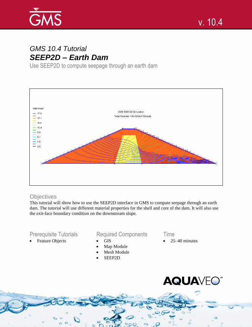
SEEP2D – Earth Dam Use SEEP2D to compute seepage through an earth dam

Objectives This tutorial will show how to use the SEEP2D interface in GMS to compute seepage through an earth

dam. The tutorial will use different material properties for the shell and core of the dam. It will also use

the exit-face boundary condition on the downstream slope.

Prerequisite Tutorials Feature Objects

Required Components GIS

Map Module

Mesh Module

SEEP2D

Time 25–40 minutes

v. 10.4



1 Introduction ......................................................................................................................... 2 2 Setup ..................................................................................................................................... 3

2.1 Program Mode .............................................................................................................. 3 2.2 Getting Started ............................................................................................................. 3 2.3 Setting the Units ........................................................................................................... 4 2.4 Saving the Project ........................................................................................................ 4

3 Creating the Conceptual Model Features ......................................................................... 5 3.1 Defining a Coordinate System ...................................................................................... 5 3.2 Creating the Corner Points ........................................................................................... 5 3.3 Creating the Arcs .......................................................................................................... 6 3.4 Creating the Polygons .................................................................................................. 6 3.5 Assigning the Material Properties and Zones ............................................................... 7

4 Assigning Boundary Conditions ........................................................................................ 8 4.1 Specified-Head Boundary Conditions .......................................................................... 8 4.2 Exit-Face Boundary Conditions ................................................................................... 9 4.3 Building the Finite Element Mesh ................................................................................ 9

5 Setting the Analysis Options............................................................................................. 11 6 Running SEEP2D .............................................................................................................. 12 7 Viewing the Solution ......................................................................................................... 12 8 Conclusion.......................................................................................................................... 13

1 Introduction

This tutorial describes the steps involved in performing a SEEP2D simulation for an

earth dam with an unsaturated zone.

The problem in this tutorial is shown in Figure 1. The problem consists of an earth dam

with anisotropic soil and a low permeability core in the interior.

110 m

18 m

17 m

8 m

22 m Core Shell

Shell kx = 46 m/yr ky = 18 m/yr Core kx = 4.5 m/yr ky = 1.8 m/yr

2 m 18 m

Figure 1 Earth dam problem

This tutorial will discuss and demonstrate creating a SEEP2D conceptual model,

mapping the model to a 2D mesh, defining conditions for both a saturated and

unsaturated zone, converting the model to SEEP2D, and running SEEP2D.



2 Setup

2.1 Program Mode

The GMS interface can be modified by selecting a Program Mode. When GMS is first

installed and runs, it is in the standard or “GMS” mode, which provides access to the

complete GMS interface, including all of the MODFLOW tools. The “GMS 2D” mode

provides a greatly simplified interface to the SEEP2D and UTEXAS codes. This mode

hides all of the tools and menu commands not related to SEEP2D and UTEXAS. This

tutorial can only be completed in the GMS 2D mode.

Once the mode is changed, GMS can be exited and restarted repeatedly and the interface

stays in the same mode until changed. Thus, it’s only necessary to change the mode once

if intending to repeatedly solve SEEP2D/UTEXAS problems. If already in GMS 2D

mode, skip ahead to the Getting Started section. If not already in GMS 2D mode, do the

following:

1. Launch GMS.

2. Select Edit | Preferences… to bring up the Preferences dialog.

3. Select “Program Mode” from the list on the left.

4. Select “GMS 2D” from the Program Mode drop-down.

5. Click OK to close the Preferences dialog.

6. Click Yes in response to the warning about all data being deleted. After a

moment, the New Project dialog will appear.

7. Click OK to close the New Project dialog.

8. Select File | Exit to exit GMS.

2.2 Getting Started

Do the following to get started:

1. If necessary, launch GMS.

2. If GMS is already running, select File | New to ensure that the program settings

are restored to their default state.

The New Project dialog will appear. This dialog is used to set up a GMS conceptual

model. A conceptual model is organized into a set of layers or groups called “coverages”.

GMS 2D allows quickly and easily defining all of the coverages needed for the

conceptual model using the New Project dialog. Most of the options seen in the window

are related to UTEXAS. For SEEP2D models, the only coverage needed is the Profile

lines coverage. This allows defining the geometry of the mesh, the boundary conditions,

and the material zones.



3. Select Create a new project and enter “Earth Dam Model” as the Conceptual

model name.

4. In the Numerical models section, turn off UTEXAS.

5. In the Create coverages section, select only Profile lines.

6. Click OK to close the New Project dialog.

A new “Earth Dam Model” conceptual model object should appear in the Project

Explorer.

2.3 Setting the Units

Before continuing, it is necessary to establish the units to be used. GMS will display the

appropriate units label next to each of the input fields as a reminder to be consistent.

1. Select Edit | Units… to open the Units dialog.

2. Click the button to the right of Length to bring up the Display Projection

dialog.

3. In both the Horizontal and Vertical sections, select “Meters” from the Units

drop-down.

4. Click OK to close the Display Projection dialog

5. Select “yr” from the Time drop-down.

6. Select “kg” from the Mass drop-down.

7. Select “N” from the Force drop-down.

8. Click OK to close the Units dialog.

2.4 Saving the Project

Before continuing, it is necessary to save the project to a GMS project file.

1. Select File | Save As… to bring up the Save As dialog.

2. Browse to the s2unc\s2unc directory.

3. Select “Project Files (*.gpr)” from the Save as type drop-down.

4. Enter “s2uncon.gpr” as the File name.

5. Click Save to create the project file and close the Save As dialog.

It is recommended to use the Save macro frequently while working on any project.



3 Creating the Conceptual Model Features

The first step in setting up the problem is to create the GIS features defining the problem

geometry. This process starts with entering a set of points corresponding to the key

locations in the geometry. Then connect the points with lines called “arcs” to define the

outline of the problem. Next, convert the arcs to a closed polygon defining the problem

domain. Once this is complete, the arcs and the polygon will be used to build the finite

element mesh and define the boundary conditions to the problem.

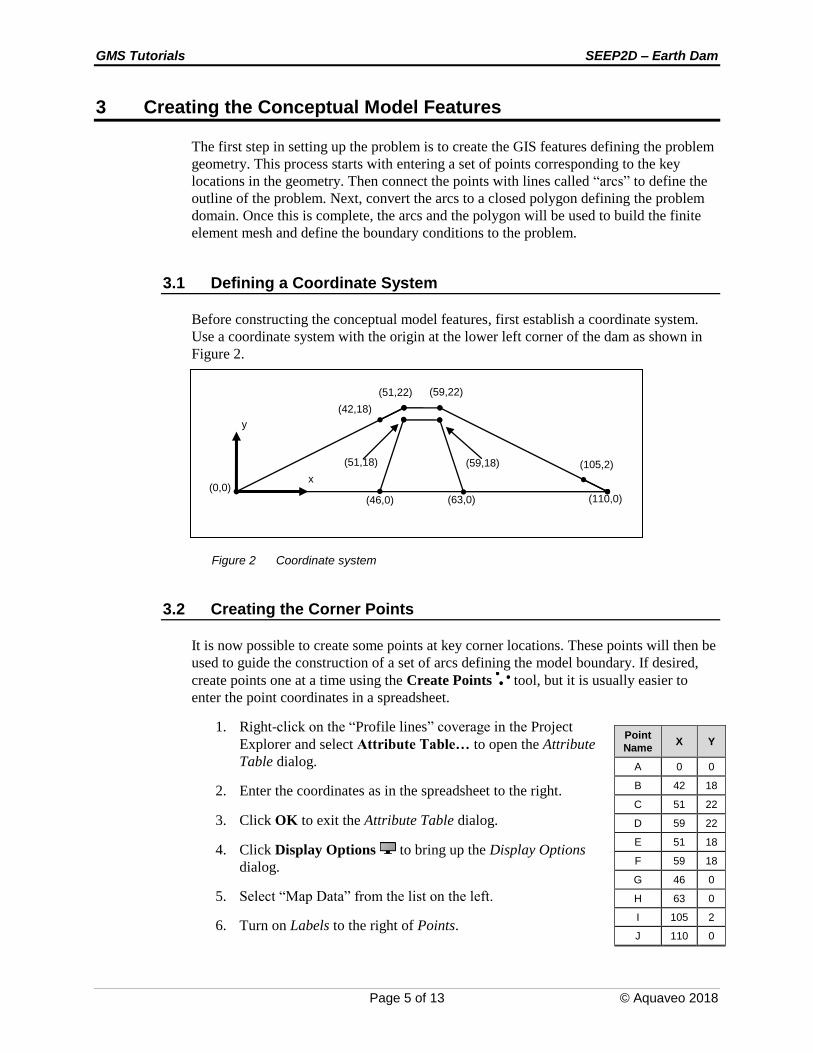
3.1 Defining a Coordinate System

Before constructing the conceptual model features, first establish a coordinate system.

Use a coordinate system with the origin at the lower left corner of the dam as shown in

Figure 2.

Figure 2 Coordinate system

3.2 Creating the Corner Points

It is now possible to create some points at key corner locations. These points will then be

used to guide the construction of a set of arcs defining the model boundary. If desired,

create points one at a time using the Create Points tool, but it is usually easier to

enter the point coordinates in a spreadsheet.

1. Right-click on the “Profile lines” coverage in the Project

Explorer and select Attribute Table… to open the Attribute

Table dialog.

2. Enter the coordinates as in the spreadsheet to the right.

3. Click OK to exit the Attribute Table dialog.

4. Click Display Options to bring up the Display Options

dialog.

5. Select “Map Data” from the list on the left.

6. Turn on Labels to the right of Points.

Point

Name X Y

A 0 0

B 42 18

C 51 22

D 59 22

E 51 18

F 59 18

G 46 0

H 63 0

I 105 2

J 110 0

x

y

(0,0) (46,0) (63,0)

(51,18) (59,18)

(42,18)

(51,22) (59,22)

(105,2)

(110,0)



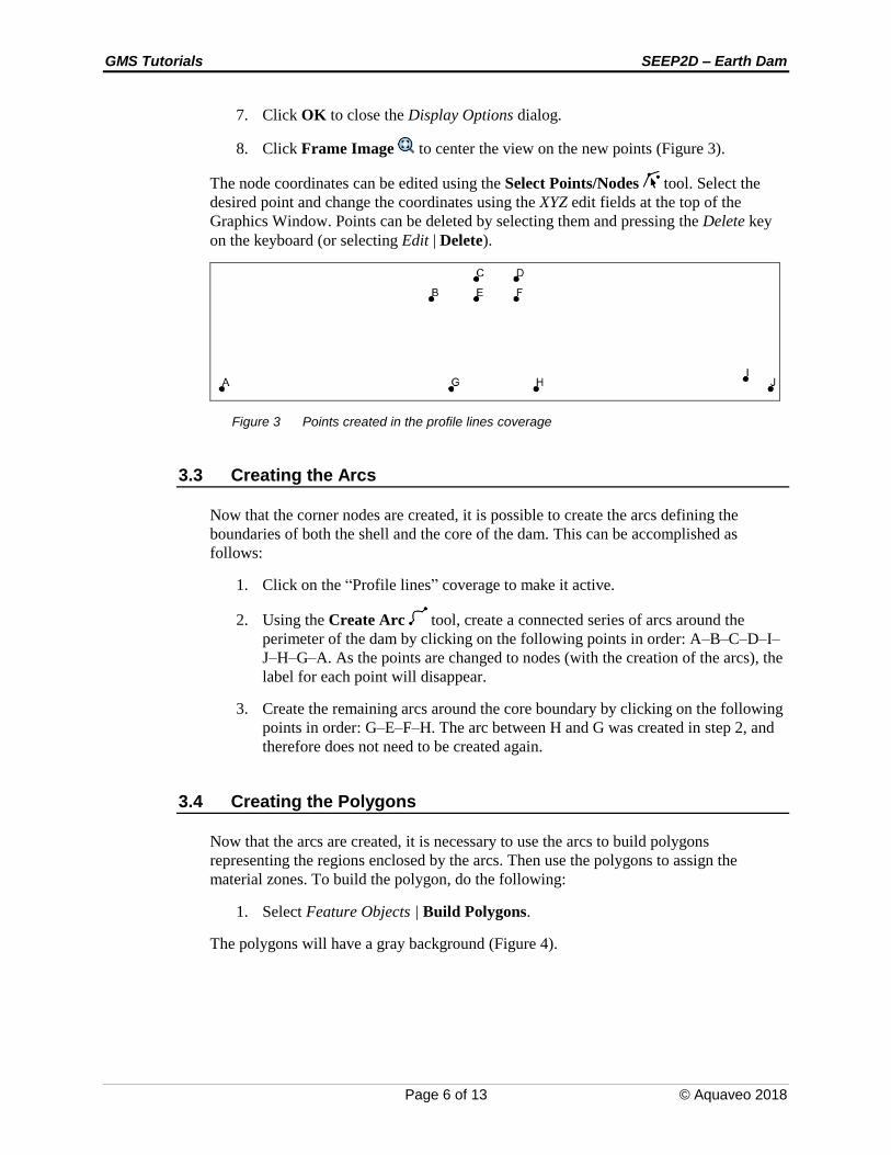
7. Click OK to close the Display Options dialog.

8. Click Frame Image to center the view on the new points (Figure 3).

The node coordinates can be edited using the Select Points/Nodes tool. Select the

desired point and change the coordinates using the XYZ edit fields at the top of the

Graphics Window. Points can be deleted by selecting them and pressing the Delete key

on the keyboard (or selecting Edit | Delete).

Figure 3 Points created in the profile lines coverage

3.3 Creating the Arcs

Now that the corner nodes are created, it is possible to create the arcs defining the

boundaries of both the shell and the core of the dam. This can be accomplished as

follows:

1. Click on the “Profile lines” coverage to make it active.

2. Using the Create Arc tool, create a connected series of arcs around the

perimeter of the dam by clicking on the following points in order: A–B–C–D–I–

J–H–G–A. As the points are changed to nodes (with the creation of the arcs), the

label for each point will disappear.

3. Create the remaining arcs around the core boundary by clicking on the following

points in order: G–E–F–H. The arc between H and G was created in step 2, and

therefore does not need to be created again.

3.4 Creating the Polygons

Now that the arcs are created, it is necessary to use the arcs to build polygons

representing the regions enclosed by the arcs. Then use the polygons to assign the

material zones. To build the polygon, do the following:

1. Select Feature Objects | Build Polygons.

The polygons will have a gray background (Figure 4).



Figure 4 Polygons with a gray background

3.5 Assigning the Material Properties and Zones

The next step is to assign the material properties and zones. This is done by creating a

material for each of the two zones in the problem and giving each material a unique

name, color, and set of hydraulic properties.

1. Click Materials to bring up the Materials dialog.

2. Rename “material_1” to “Shell” in the Name column of the spreadsheet.

3. In the Color/Pattern column in row 1, click the down arrow to the right of the

wide color button and select “light orange” from the list of swatches.

4. On row 1:

Enter “46” in the k1 column.

Enter “18” in the k2 column.

Enter “-0.3” in the Sat/Unsat linear front ho column.

Enter “0.001” in the Sat Unsat linear front kro column.

5. Create a new material by entering “Core” in the Name column of the blank row

(marked with a “*”) at the bottom of the spreadsheet. The row is now numbered

“2”.

6. In the Color/Pattern column in row 2, select “pale green” from the list of

swatches.

7. On row 2:

Enter “4.6” in the k1 column.

Enter “1.8” in the k2 column.

Enter “-1.2” in the Sat/Unsat linear front ho column.

Enter “0.001” in the Sat Unsat linear front kro column.

8. Click OK to close the Materials dialog.

Note that both polygons are currently associated with the “Shell” material (Figure 5).

Change the material assigned to the core polygon to the new “Core” material.



Figure 5 Both polygons are the same material

9. Using the Select Polygons tool, double-click inside the core polygon to bring

up the Attribute Table dialog.

10. In the Material column of the spreadsheet, select “Core” from the drop-down.

11. Click OK to close the Attribute Table dialog.

12. Click anywhere outside the polygons in the Graphics Window to unselect the

polygon.

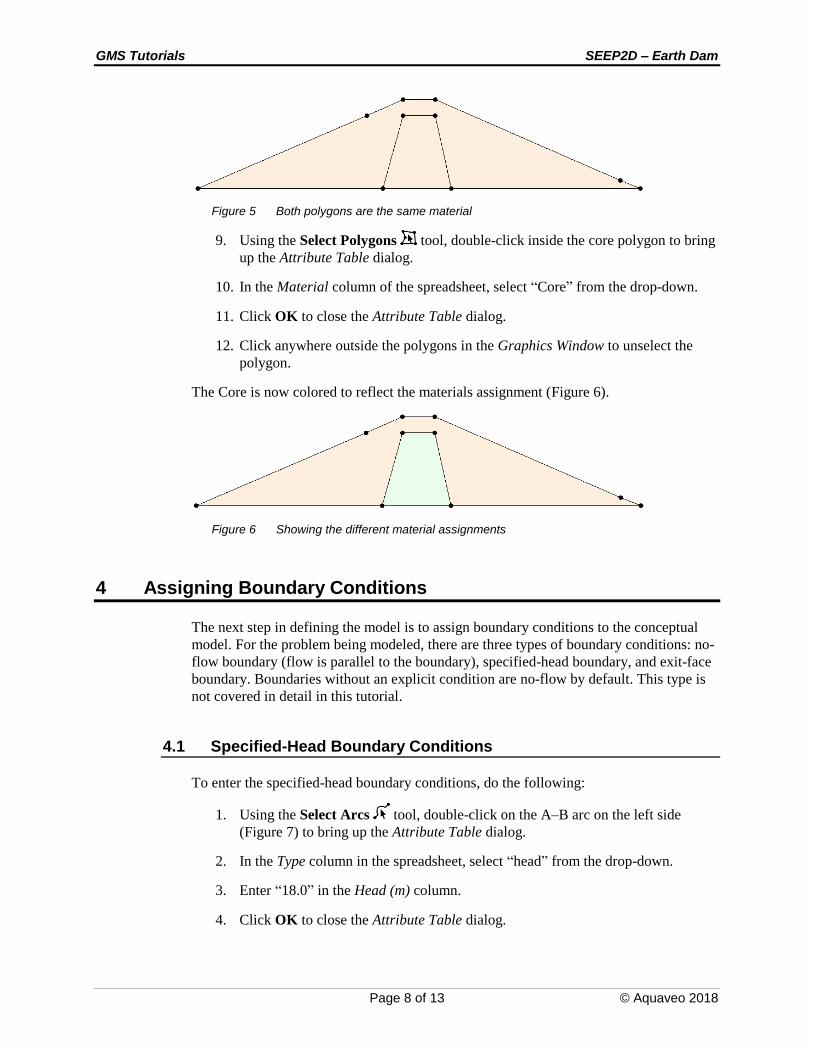
The Core is now colored to reflect the materials assignment (Figure 6).

Figure 6 Showing the different material assignments

4 Assigning Boundary Conditions

The next step in defining the model is to assign boundary conditions to the conceptual

model. For the problem being modeled, there are three types of boundary conditions: no-

flow boundary (flow is parallel to the boundary), specified-head boundary, and exit-face

boundary. Boundaries without an explicit condition are no-flow by default. This type is

not covered in detail in this tutorial.

4.1 Specified-Head Boundary Conditions

To enter the specified-head boundary conditions, do the following:

1. Using the Select Arcs tool, double-click on the A–B arc on the left side

(Figure 7) to bring up the Attribute Table dialog.

2. In the Type column in the spreadsheet, select “head” from the drop-down.

3. Enter “18.0” in the Head (m) column.

4. Click OK to close the Attribute Table dialog.



5. Repeat steps 1–4 with the I–J arc on the lower right side (Figure 7), entering

“2.0” in the Head (m) column.

6. Click anywhere outside of the polygons to unselect the arc.

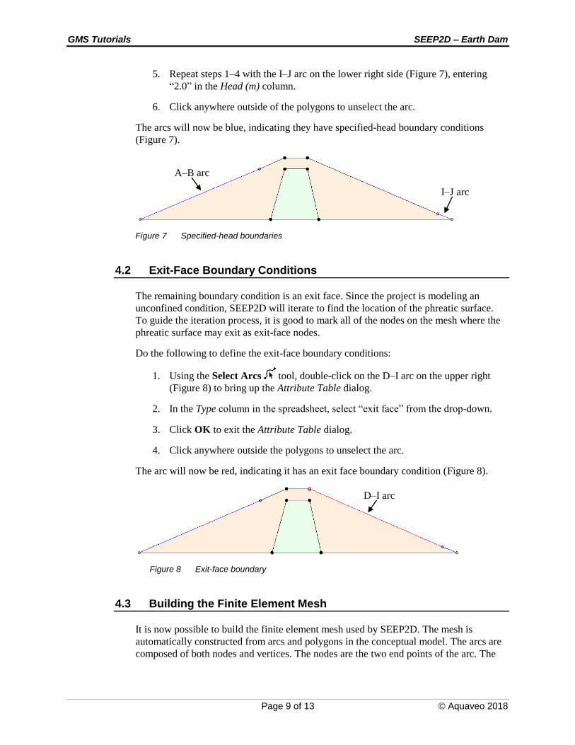
The arcs will now be blue, indicating they have specified-head boundary conditions

(Figure 7).

Figure 7 Specified-head boundaries

4.2 Exit-Face Boundary Conditions

The remaining boundary condition is an exit face. Since the project is modeling an

unconfined condition, SEEP2D will iterate to find the location of the phreatic surface.

To guide the iteration process, it is good to mark all of the nodes on the mesh where the

phreatic surface may exit as exit-face nodes.

Do the following to define the exit-face boundary conditions:

1. Using the Select Arcs tool, double-click on the D–I arc on the upper right

(Figure 8) to bring up the Attribute Table dialog.

2. In the Type column in the spreadsheet, select “exit face” from the drop-down.

3. Click OK to exit the Attribute Table dialog.

4. Click anywhere outside the polygons to unselect the arc.

The arc will now be red, indicating it has an exit face boundary condition (Figure 8).

Figure 8 Exit-face boundary

4.3 Building the Finite Element Mesh

It is now possible to build the finite element mesh used by SEEP2D. The mesh is

automatically constructed from arcs and polygons in the conceptual model. The arcs are

composed of both nodes and vertices. The nodes are the two end points of the arc. The

D–I arc

A–B arc

I–J arc



vertices are intermediate points between the nodes. The gaps between vertices are called

edges.

At this point, all of the arcs have one edge and zero vertices. When mapping to a 2D

mesh, the density of the elements in the interior of the mesh is controlled by the edge

spacing along the arcs. Thus, it is necessary to subdivide the arcs to create appropriately

sized edges.

1. Using the Select Arcs tool, select all of the arcs by dragging a box that

encloses all of the arcs.

2. Select Feature Objects | Redistribute Vertices… to bring up the Redistribute

Vertices dialog.

3. Select “Specified spacing” from the Specify drop-down.

4. Enter “2.5” for the Average spacing.

5. Click OK to close the Redistribute Vertices dialog.

6. Switch to the Select Vertices tool.

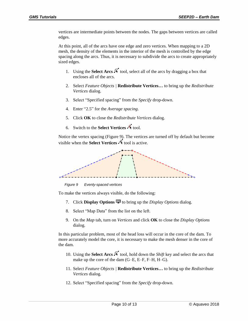
Notice the vertex spacing (Figure 9). The vertices are turned off by default but become

visible when the Select Vertices tool is active.

Figure 9 Evenly-spaced vertices

To make the vertices always visible, do the following:

7. Click Display Options to bring up the Display Options dialog.

8. Select “Map Data” from the list on the left.

9. On the Map tab, turn on Vertices and click OK to close the Display Options

dialog.

In this particular problem, most of the head loss will occur in the core of the dam. To

more accurately model the core, it is necessary to make the mesh denser in the core of

the dam.

10. Using the Select Arcs tool, hold down the Shift key and select the arcs that

make up the core of the dam (G–E, E–F, F–H, H–G).

11. Select Feature Objects | Redistribute Vertices… to bring up the Redistribute

Vertices dialog.

12. Select “Specified spacing” from the Specify drop-down.



13. Enter “1.0” for the Average spacing.

14. Click OK to close the Redistribute Vertices dialog.

At this point, it is possible to construct the mesh.

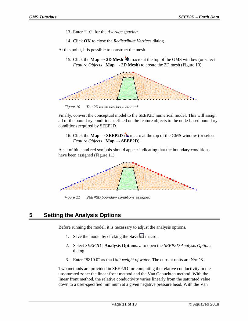
15. Click the Map → 2D Mesh macro at the top of the GMS window (or select

Feature Objects | Map → 2D Mesh) to create the 2D mesh (Figure 10).

Figure 10 The 2D mesh has been created

Finally, convert the conceptual model to the SEEP2D numerical model. This will assign

all of the boundary conditions defined on the feature objects to the node-based boundary

conditions required by SEEP2D.

16. Click the Map → SEEP2D macro at the top of the GMS window (or select

Feature Objects | Map → SEEP2D).

A set of blue and red symbols should appear indicating that the boundary conditions

have been assigned (Figure 11).

Figure 11 SEEP2D boundary conditions assigned

5 Setting the Analysis Options

Before running the model, it is necessary to adjust the analysis options.

1. Save the model by clicking the Save macro.

2. Select SEEP2D | Analysis Options… to open the SEEP2D Analysis Options

dialog.

3. Enter “9810.0” as the Unit weight of water. The current units are N/m^3.

Two methods are provided in SEEP2D for computing the relative conductivity in the

unsaturated zone: the linear front method and the Van Genuchten method. With the

linear front method, the relative conductivity varies linearly from the saturated value

down to a user-specified minimum at a given negative pressure head. With the Van



Genuchten method, the Van Genuchten parameters are used to define the variation of the

relative conductivity in the unsaturated zone. Both methods are described in detail in the

“SEEP2D Primer”. For this tutorial, use the linear front option.

4. In the Model type section, select Saturated/Unsaturated with linear front.

5. Click OK to exit the SEEP2D Analysis Options dialog.

6 Running SEEP2D

It is now possible to run SEEP2D. Before running SEEP2D, it is important to make sure

all of the changes have been saved:

1. Click Save .

2. Click the Run SEEP2D macro (or select SEEP2D | Run SEEP2D) to bring

up the Seep2d model wrapper dialog.

3. When the solution is finished, turn on Read solution on exit and click Close to

close the Seep2d model wrapper dialog.

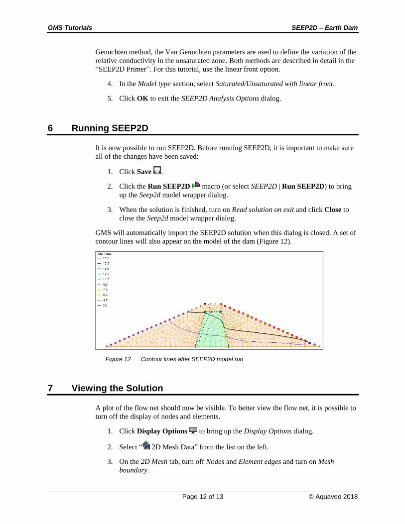
GMS will automatically import the SEEP2D solution when this dialog is closed. A set of

contour lines will also appear on the model of the dam (Figure 12).

Figure 12 Contour lines after SEEP2D model run

7 Viewing the Solution

A plot of the flow net should now be visible. To better view the flow net, it is possible to

turn off the display of nodes and elements.


2. Select “ 2D Mesh Data” from the list on the left.

3. On the 2D Mesh tab, turn off Nodes and Element edges and turn on Mesh

boundary.




Note that there are only a small number of flow lines (Figure 13). GMS determines the

number of flow lines to display based on how closely spaced the equipotential lines are

in one of the materials. By default, the interval is computed based on the Shell material.

Figure 13 Less cluttered view with nodes and elements off and mesh on

To base the number of flow lines on the Core material, do the following:


2. Select “ 2D Mesh Data” from the list on the left.

3. On the SEEP2D tab, select “Core” from the Base Material drop-down.

4. Make sure Phreatic surface is turned on.


Flow lines are now visible through the model as well as the phreatic surface (Figure 14).

Figure 14 Flow lines and phreatic surface visible

8 Conclusion

This concludes the “SEEP2D – Earth Dam” tutorial. The following topics were

discussed and demonstrated:

SEEP2D can perform 2D unconfined flow modeling.

SEEP2D problems can be set up quickly and easily using the conceptual model

approach.

Display a flow net and the phreatic surface in GMS.

Documents

GMS Tutorials SEEP2D v. 10gmstutorials-10.4.aquaveo.com/SEEP2D-EarthDam.pdf · 2018-09-18 · Figure 5 Both polygons are the same material 9. Using the Select Polygons tool, double-click