Fukushima LaboratoryProf. Dr. Edwardo F. Fukushima

Bio-Inspired Robotics LaboratoryProf. Dr. Fumiya Iida

Referees: Author: Yongjae KimProf. Dr. Edwardo F. FukushimaProf. Dr. Fumiya Iida

Supervised by: Submitted on: June 27, 2014Dr. Surya G. NurzamanXiaoxiang Yu

Goal-directedMulti-modal Locomotion of

Curved Beam HoppingRobot

Master’s Thesis

Tokyo Institute of TechnologyGraduate School of Science and Engineering

Department of Mechanical and Aerospace Engineering

Eidgenossische Technische Hochschule ZurichDepartment of Mechanical and Process Engineering

Institute of Robotics and Intelligent Systems

Contents

Abstract iii

Published work v

Acknowledgements vii

1 Introduction 1

2 Dynamical coupling between mechanical dynamics andAttractor Selection Mechanism 3

3 Curved Beam Hopping Robot and the simulation model 53.1 Numerical model of Curved Beam Hopping Robot . . . . . . . . . . 53.2 Ground Contact Model . . . . . . . . . . . . . . . . . . . . . . . . . 7

4 Analysis of the robot behavior 84.1 Fast Fourier Transform on the behavior . . . . . . . . . . . . . . . . 84.2 Parameters for behavioral analysis . . . . . . . . . . . . . . . . . . . 94.3 Behavioral analysis . . . . . . . . . . . . . . . . . . . . . . . . . . . . 10

5 Goal-directed multi-modal locomotion 185.1 Experimental setting . . . . . . . . . . . . . . . . . . . . . . . . . . . 185.2 Experiment results . . . . . . . . . . . . . . . . . . . . . . . . . . . . 20

6 Real-world experiment 256.1 Behavioral analysis . . . . . . . . . . . . . . . . . . . . . . . . . . . . 256.2 Experimental setting . . . . . . . . . . . . . . . . . . . . . . . . . . . 266.3 Experiment results . . . . . . . . . . . . . . . . . . . . . . . . . . . . 27

7 Conclusion 29

Bibliography 31

Statement of authorship 35

i

ii

Abstract

In order for a robotic system to survive in different environments, multi-modality,i.e. the ability to have multiple modes of locomotion with a single robot, is in-dispensable. To properly exploit this capability, a coupling between the mechan-ical dynamics of the robot and a suitable controller is important, including whenit comes to specific task such as goal-directed locomotion. This work focuses onthe coupling between a control structure known as Attractor Selection Mechanism(ASM) and the mechanical dynamics of an exemplary robotic system: Curved BeamHopping Robot (CBHR). ASM uses internal stochastic perturbation and sensoryinput to control the robot so that it can gracefully shift between distinct attractors.Because of the dynamic coupling between the ASM attractors and the attractorsof the mechanical dynamics which represent distinct locomotion modes, the robotachieves goal-directed behavior, even in different environmental condition. Theefficacy of the approach is shown by simulation and real-world experiment.

iii

iv

Appended papers

This thesis is based on the following papers.

Paper I

Nurzaman S. G., Yu X., Kim Y. and Iida F., “Guided Self-Organization in aDynamic Embodied System Based on Attractor Selection Mechanism,” Entropy,16(5) : 2592-2610, 2014

Paper II

Nurzaman S. G., Yu X., Kim Y. and Iida F., “Goal directed multimodal locomotionthrough coupling between mechanical and attractor selection dynamics,” Bioinspi-ration & Biomimetics, Revised

v

vi

Acknowledgements

This work was carried out as a part of the student exchange program between ETHZurich and Tokyo Institute of Technology (Tokyo Tech.). I would like to thank bothfor allowing me to study here at ETH Zurich. I could not fulfilled this work withoutfinancial support from ETH Zurich, which also approved by Tokyo Tech.

Dr. Surya G. Nurzaman supervised this work and always gave me helpful advice inevery aspect including research affairs and writing paper, etc. I hope I could learnby heart at least a part of knowledge what he taught me during the period I havestayed here.

I also thank Xiaoxiang Yu who had supervised me and fully supported my work un-til he found his new job. I’ll keep my fingers crossed for his future career in industry.

I cannot thank Prof. Fumiya Iida enough, who generously allowed me to study atBIRLab and gave me a lot of critical advice concerning actual research, studying inAcademia. He always enlightened me with his insightful and convincing commentsat every meeting.

Finally, I would like to thank all crew in BIRLab with whom I could have interestingdiscussions and feel at home. It was my utmost pleasure to be here with them.

vii

viii

Chapter 1

Introduction

Animals are able to versatilely move in various unstructured environments for theiraims in livings, e.g., foraging, avoiding predators, and mating. Developing and uti-lizing multi-modal locomotion, the ability to perform multiple locomotion modeswith a single body, is one of the most important characteristics to achieve suchtasks. To understand the mechanism how animals utilize this multi-modality, anumber of researches have been done. For example, some of the researches focus onunderstanding how to imitate multiple locomotion abilities of animals like seabirds,salamanders and frogs, i.e. aerial, terrestrial and aquatic [1–4].

Among various researches concerning multi-modal locomotion, the ones which focuson terrestrial environments have gained a lot of attentions. In multi-legged roboticsresearch, some approaches to achieve multi-modal locomotion such as walking andrunning by using single robot have been proposed [5, 6]. Many studies on leggedrobots also focus on single legged hopping machines, claiming its potential not onlyto operate in unstructured environments but also to tackle unique challenges likeactive balance, use of elasticity for mechanical oscillations [7]. It is shown that it ispossible to achieve different locomotion modes with single legged robot, i.e. hoppingand sliding, by using different control schemes for stance and flight phases [8].

However, multi-modal locomotion should be understood on the basis of embodiedsystem, i.e. systems with mechanical bodies which are physically embedded in en-vironment [10]. The behaviors of embodied system cannot be considered as solelythe outcome of internal control such as brain and central nervous system in biolog-ical system. They are also affected by both the environments and morphologies ofthe system. That is, behaviors of embodied system must be seen as the results ofself-organization through the interaction between internal control structure, bodyand environment [10,11,14,15].

It has also been suggested that in non-trivial structure like tensegrity, the richand complex mechanical dynamics coming from the body-environment interactionsshould be exploited to achieve locomotion [12, 13]. In fact, it is argued that thebody morphology and its interactions with the environment can simplify the con-trol structure by taking over some of the processes normally attributed to control:a phenomenon commonly referred to as morphological computation [14, 32]. It is,however, not trivial to dynamically couple these components properly such thata robot is able to take advantage of its multiple locomotion modes to accomplishuseful tasks.

In order for a robot to achieve useful locomotion behavior like goal directed locomo-

1

Chapter 1. Introduction 2

tion, the approaches based on Central Pattern Generators (CPGs) are commonlytaken. Inspired by neural mechanism in animals, CPGs are used to produce basicrhythmic patterns, and in general require a priori knowledge about the body mor-phology, i.e. the limbs participating in the locomotion process [2, 30, 31]. In thesame line of research, some studies propose CPGs-based approach to explore andtake advantage of different locomotion modes in an on-line manner which make asystem be adaptive to different body morphology and environments. Influenced byresearches on chaotic neural dynamics in animal nervous system, the use of adap-tive chaotic search to explore different mechanical dynamics like body-environmentdynamics is proposed [33]. In the study, the capability to stabilize on one of thelocomotion modes which matches given criteria is emphasized. However, in thiswork, the focus is on stochastic dynamics due to two main reasons: firstly, simpleanimals, which do not even have nervous systems, are known to exploit stochasticdynamics and able to achieve meaningful behaviors like goal-directed locomotionwithout a priori knowledge of the limbs [9,17]; secondly, it has been suggested thatcertain stochastic animal behaviors evolved through the interaction with environ-ments, showing the importance of a coupled dynamics [34].

The main goal of this thesis is to propose an approach to enable a robotic systemto achieve goal-directed multi-modal locomotion in a variety of environments. Thepith of the approach is to couple the mechanical dynamics of the system and astochastic controller, i.e. Attractor Selection Mechanism (ASM). ASM is a controlmethod utilizing internal stochastic perturbation, which is inspired by probably thesimplest animal, bacteria [9, 16–20]. The robotic system used in this thesis is aCurved Beam Hopping Robot, which possesses rich and complex dynamics depend-ing on its environment despite its simple actuation mechanism [21,22]. By utilizingits multi-modal locomotion, the robot is hypothesized to be able to reach partic-ular target even in unstructured environments, depending on internally generatedstochastic perturbation and sensory input.

The rest of this thesis is organized as follows. Firstly, the concept used in this thesisincluding coupling between the mechanical dynamics and ASM will be introduced.Secondly, configurations on simulation of the robot used in this thesis, the CurvedBeam Hopping Robot, will be presented. Thirdly, the analyses based on the system’sdynamics will be discussed. Afterwards, the results of experiment of goal-directedscheme will be shown with consequential discussion, which followed by the result ofreal-world experiment. Finally, conclusive remarks will be presented.

Chapter 2

Dynamical coupling betweenmechanical dynamics andAttractor SelectionMechanism

ASM is inspired by various scales of biological system utilizing noise such as biomolecules,cells, brain [9, 10]. A simple model was proposed to explain the underlying mecha-nism, which represented by Langevin equation as:

s = −∇U(s(t))A(t) + ε(t) (2.1)

where s(t) and −∇U(s) are the state and the dynamics of the system at time t,respectively, and ε(t) is the noise term. ε(t) decides the tendency of the dynamics tobe deterministic or stochastic while the state s(t) of ASM is used as the actuationcommand. The sensory feedback function A(t) represents suitability of the stateto desirable goal. More specifically, from the equation −∇U(s(t))A(t) becomesdominant over ε(t) when A(t) is large, which means the system becomes moredeterministic. Conversely, when A(t) is small, ε(t) becomes dominant, and thesystem gets more stochastic.

3

Chapter 2. Dynamical coupling between mechanical dynamics andAttractor Selection Mechanism 4

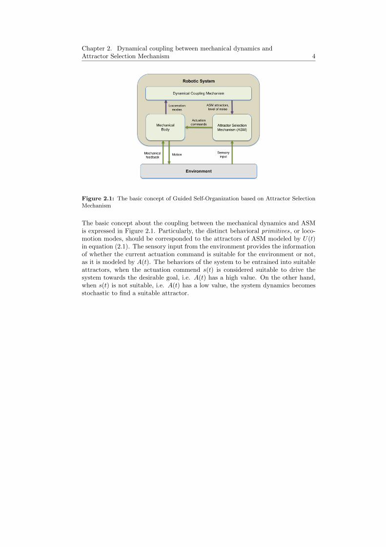
Figure 2.1: The basic concept of Guided Self-Organization based on Attractor SelectionMechanism

The basic concept about the coupling between the mechanical dynamics and ASMis expressed in Figure 2.1. Particularly, the distinct behavioral primitives, or loco-motion modes, should be corresponded to the attractors of ASM modeled by U(t)in equation (2.1). The sensory input from the environment provides the informationof whether the current actuation command is suitable for the environment or not,as it is modeled by A(t). The behaviors of the system to be entrained into suitableattractors, when the actuation commend s(t) is considered suitable to drive thesystem towards the desirable goal, i.e. A(t) has a high value. On the other hand,when s(t) is not suitable, i.e. A(t) has a low value, the system dynamics becomesstochastic to find a suitable attractor.

Chapter 3

Curved Beam HoppingRobot and the simulationmodel

The embodied system used as a paradigmatic platform in this thesis is a simulatedCurved Beam Hopping Robot based on our previous research [21, 22]. The modelof the Curved Beam Hopping Robot and its mechanical dynamics are explainedin following sections. The model is implemented by using standard components ofMATLAB SimmechanicsTM [26].

3.1 Numerical model of Curved Beam HoppingRobot

(a) Curved Beam Hopping Robot(CBHR) (b) Modeled CBHR

Figure 3.1: The embodied system studied in this thesis

Figure 3.1(a) shows the physical Curved Beam Hopping Robot, which is similar tothe one used in our previous research [21,22]. The only thing different from previousis the fact that current version has only one rotating object on its right side of thehead. The robot consists of a curved aluminum beam, which is attached to a large

5

Chapter 3. Curved Beam Hopping Robot and the simulation model 6

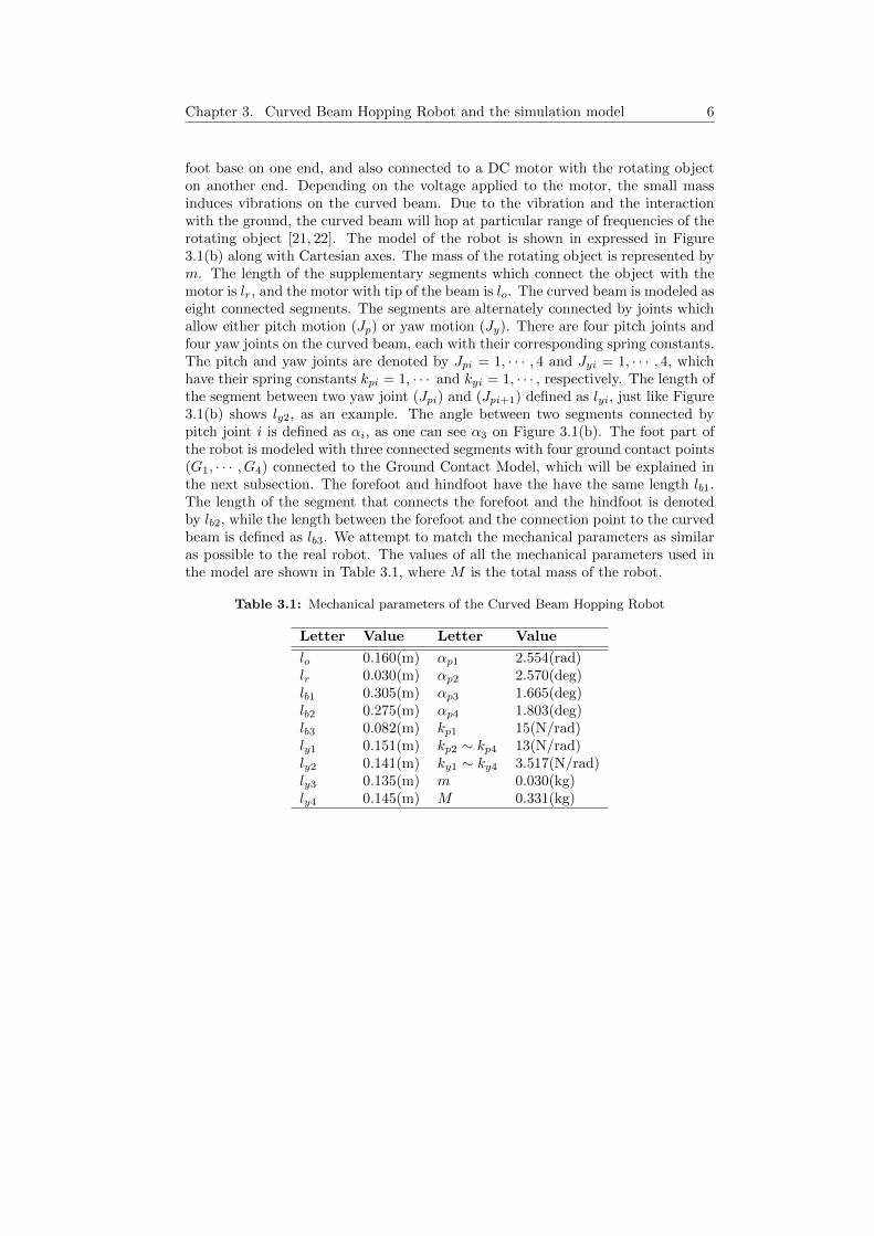
foot base on one end, and also connected to a DC motor with the rotating objecton another end. Depending on the voltage applied to the motor, the small massinduces vibrations on the curved beam. Due to the vibration and the interactionwith the ground, the curved beam will hop at particular range of frequencies of therotating object [21, 22]. The model of the robot is shown in expressed in Figure3.1(b) along with Cartesian axes. The mass of the rotating object is represented bym. The length of the supplementary segments which connect the object with themotor is lr, and the motor with tip of the beam is lo. The curved beam is modeled aseight connected segments. The segments are alternately connected by joints whichallow either pitch motion (Jp) or yaw motion (Jy). There are four pitch joints andfour yaw joints on the curved beam, each with their corresponding spring constants.The pitch and yaw joints are denoted by Jpi = 1, · · · , 4 and Jyi = 1, · · · , 4, whichhave their spring constants kpi = 1, · · · and kyi = 1, · · · , respectively. The length ofthe segment between two yaw joint (Jpi) and (Jpi+1) defined as lyi, just like Figure3.1(b) shows ly2, as an example. The angle between two segments connected bypitch joint i is defined as αi, as one can see α3 on Figure 3.1(b). The foot part ofthe robot is modeled with three connected segments with four ground contact points(G1, · · · , G4) connected to the Ground Contact Model, which will be explained inthe next subsection. The forefoot and hindfoot have the have the same length lb1.The length of the segment that connects the forefoot and the hindfoot is denotedby lb2, while the length between the forefoot and the connection point to the curvedbeam is defined as lb3. We attempt to match the mechanical parameters as similaras possible to the real robot. The values of all the mechanical parameters used inthe model are shown in Table 3.1, where M is the total mass of the robot.

Table 3.1: Mechanical parameters of the Curved Beam Hopping Robot

Letter Value Letter Value

lo 0.160(m) αp1 2.554(rad)lr 0.030(m) αp2 2.570(deg)lb1 0.305(m) αp3 1.665(deg)lb2 0.275(m) αp4 1.803(deg)lb3 0.082(m) kp1 15(N/rad)ly1 0.151(m) kp2 ∼ kp4 13(N/rad)ly2 0.141(m) ky1 ∼ ky4 3.517(N/rad)ly3 0.135(m) m 0.030(kg)ly4 0.145(m) M 0.331(kg)

7 3.2. Ground Contact Model

3.2 Ground Contact Model

Each contact point G1, · · · , G4 to the ground on the foot part of the robot is con-nected to the Ground Contact Model. We use the following contact model:

fxi = −kxi(xi − xi0)− dxxi (3.1)

fyi = −kyi(yi − yi0)− dy yi (3.2)

fzi =

{fzci − fg (if zi ≤ 0)−fg (otherwise)

(3.3)

where fg is the gravitational force, and the z-directional reaction force fzci is definedas follows:

fzci =

{−kzzi − dz zi (if −kzzi − dz zi ≥ 0)

0 (otherwise)(3.4)

The model assumes that the ground is adequately soft so that the contact pointscan be placed below the ground. Reaction forces from the ground to the contactpoints only exert when they are below the ground, while there is no pulling forcetowards the ground when the velocity of Gi is positive [27]. kx, ky and kz are thespring coefficient at points along the x, y and z-direction respectively, while dx,dy, and dz are corresponding damping coefficients. The values of these parameterson Ground Contact Model are shown in Table 3.2. Note that kx, ky, dx, dy aretunable parameters with two values for each.

Table 3.2: Parameters of Ground Contact Model (GCM)

Letter Value Letter Value

kx 5, 10(N/m) dx 5, 10(N· s/m)ky 5, 10(N/m) dy 5, 10(N· s/m)kz 105(N/m) dz 10(N· s/m)

Chapter 4

Analysis of the robotbehavior

In this chapter, using a numerical model described in the previous chapter, we definehow to analyze the robot’s behaviors depending rotating frequency. More specif-ically: first, in order to know at which rotating frequency the robot shows whichbehavior, we run several 10-second-simulations at constant rotating frequency; sec-ond, Fast Fourier Transform and specially defined parameters are used to analyzethe behaviors. Finally, the behavioral properties of the robot based on the analyz-ing methods are shown with corresponding figures.

4.1 Fast Fourier Transform on the behavior

Figure 4.1: How to calculate Fast Fourier Transform on the behavior

Even the rotating frequency is constant, because of the curved beam’s elasticity,the motion of the head part of the robot (let us call this as headpoint) has variousoscillation modes. To find the dominant mode among them and its amplitude, wecalculate Fast Fourier Transform (FFT) on ~p in Figure 4.1, based on the robot’scoordinate (O-xryrzr).

8

9 4.2. Parameters for behavioral analysis

4.2 Parameters for behavioral analysis

The Curved Beam Hopping Robot used in this project has various behavioral pat-terns depending on the angular frequency of the rotating object. In order to describesuch properties, we define a simple 2-dimensional model on Figure 4.2, along withabsolute Cartesian space:

Figure 4.2: The model of 2-dimensional motion of the system

Here, ~pi is a unit vector which represents the robot’s orientation at time ti. Asalso shown in the figure, ~qi is a displacement vector of the robot within the timegap ti − ti−1. The angle φi and θi are defined as the orientation angle of ~pi and ~qirespectively, based on the absolute coordinate described on Figure 4.2. Therefore,the mathematical definitions of the two vectors are expressed as (4.1) and (4.2).

~pi = (1,∠φi) (4.1)

~qi = (Di,∠θi) (4.2)

where Di represents the magnitude of ~qi. Furthermore, in order to characterize themotion for each angular frequency, we generalize the tendency of the samples ateach time ti (i = 1, · · · , n) in particular frequency. Specifically, we define ~pm and~qm, the average vectors on ~pi and ~qi (i = 1, · · · , n), which is shown as (4.3) and(4.4).

~pm =1n

∑ni=1 ~pi∥∥ 1

n

∑ni=1 ~pi

∥∥ = (1, φm) (4.3)

~qm =1n

∑ni=1 ~qi∥∥ 1

n

∑ni=1 ~qi

∥∥ = (Dm, θm) (4.4)

where Dm, θm and φm are defined as average value on Di, θi and φi, respectively.Note that ~pi is normalized because magnitude of the vector has no physical meaning.

Chapter 4. Analysis of the robot behavior 10

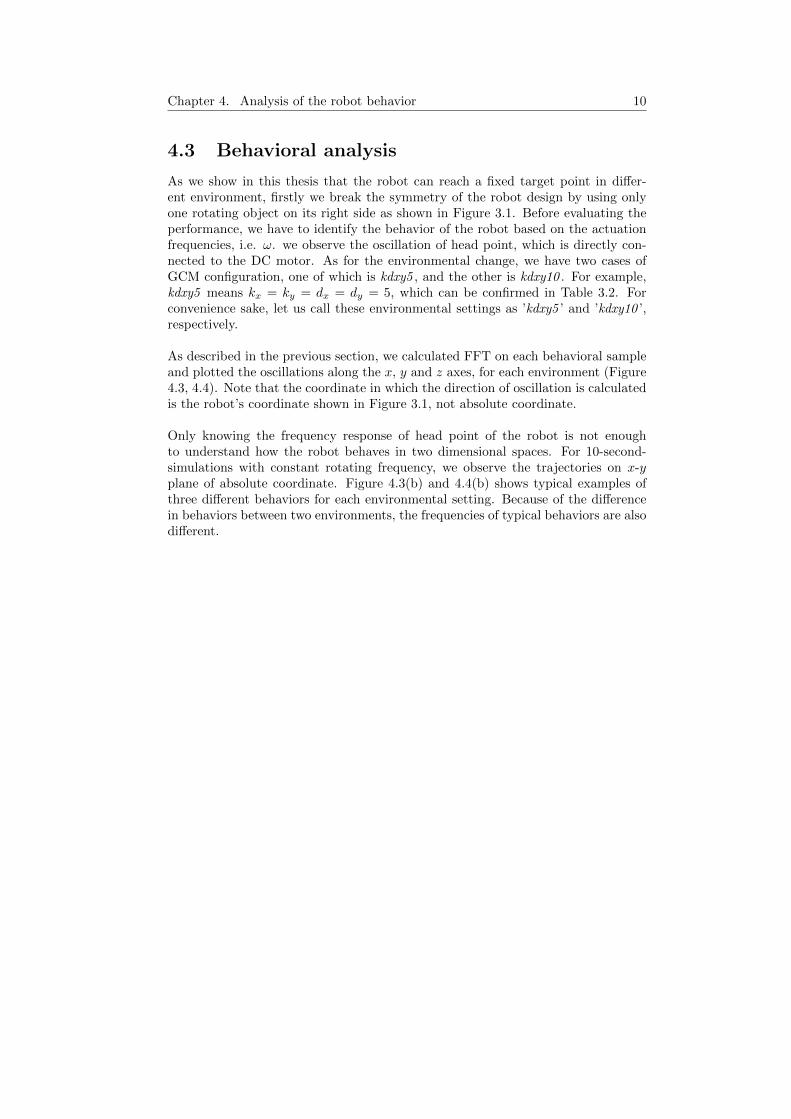
4.3 Behavioral analysis

As we show in this thesis that the robot can reach a fixed target point in differ-ent environment, firstly we break the symmetry of the robot design by using onlyone rotating object on its right side as shown in Figure 3.1. Before evaluating theperformance, we have to identify the behavior of the robot based on the actuationfrequencies, i.e. ω. we observe the oscillation of head point, which is directly con-nected to the DC motor. As for the environmental change, we have two cases ofGCM configuration, one of which is kdxy5 , and the other is kdxy10 . For example,kdxy5 means kx = ky = dx = dy = 5, which can be confirmed in Table 3.2. Forconvenience sake, let us call these environmental settings as ’kdxy5 ’ and ’kdxy10 ’,respectively.

As described in the previous section, we calculated FFT on each behavioral sampleand plotted the oscillations along the x, y and z axes, for each environment (Figure4.3, 4.4). Note that the coordinate in which the direction of oscillation is calculatedis the robot’s coordinate shown in Figure 3.1, not absolute coordinate.

Only knowing the frequency response of head point of the robot is not enoughto understand how the robot behaves in two dimensional spaces. For 10-second-simulations with constant rotating frequency, we observe the trajectories on x-yplane of absolute coordinate. Figure 4.3(b) and 4.4(b) shows typical examples ofthree different behaviors for each environmental setting. Because of the differencein behaviors between two environments, the frequencies of typical behaviors are alsodifferent.

11 4.3. Behavioral analysis

(a) The dominant amplitudes of head point’s oscillation

(b) Behavior examples with fixed rotating frequencies

Figure 4.3: kdxy5

Chapter 4. Analysis of the robot behavior 12

(a) The dominant amplitudes of head point’s oscillation

(b) Behavior examples with fixed rotating frequencies

Figure 4.4: kdxy10

13 4.3. Behavioral analysis

In Figure 4.3, it can be seen that up until approximately ω = 20(rad/s), the ten-dency of the oscillation barely changes so that does not affect movement of the robot.Despite the fact that in y direction the maximum oscillation amplitude increases atthe frequency below ω = 20(rad/s), as we can confirm in the figure, the robot barelymoves in that frequency range, as shown in Figure 4.3(b), and 4.4(b). This meansin the frequency range below ω = 20(rad/s), the oscillation of head point cannotinduce the movement of the foot. However, above ω = 20(rad/s), the amplitudestarts to increase. In kdxy5 , From ω = 20(rad/s) to ω = 45(rad/s), the oscillationamplitudes along the z direction are almost always higher than those along the xand y directions. However in higher frequency range, i.e. ω = 45 ∼ 50(rad/s),the amplitudes along the x and y directions tend to be higher than that of the zdirection.

Similar tendency can be seen in the case of kdxy10 . However, the most significantdifference from in kdxy5 is the fact that the amplitudes along x and y direction gethigher than that of z direction from ω = 35(rad/s), not from ω = 45(rad/s) Thatis, the tendency to increase in the x and y directional amplitudes starts aroundω = 35(rad/s) in kdxy10 , not like in kdxy5 . It is interesting to notice, In both envi-ronment, that this change of tendency in amplitudes is similar to the phenomenonof torsional and longitudinal oscillation of the robot used in our previous research,which has two rotating object on both side [21, 22]. However, since in this thesisproject the robot is asymmetric, the amplitudes along the x and y direction becomesignificant, rather than along z direction.

Chapter 4. Analysis of the robot behavior 14

20 25 30 35 40 45 50

0

0.05

0.1

0.15

0.2

0.25

Dm

(m

)

kxy

=dxy

=5

20 25 30 35 40 45 50

0

0.05

0.1

0.15

0.2

0.25

ω (rad/s)

Dm

(ra

d)

kxy

=dxy

=5

(a) Dm

20 25 30 35 40 45 50−6

−4

−2

0

2

4

6

θm

(ra

d)

kxy

=dxy

=5

20 25 30 35 40 45 50−6

−4

−2

0

2

4

6

ω (rad/s)

θm

(ra

d)

kxy

=dxy

=5

(b) θm

20 25 30 35 40 45 50−4

−3

−2

−1

0

1

2

3

4

φm

(ra

d)

kxy

=dxy

=5

20 25 30 35 40 45 50−4

−3

−2

−1

0

1

2

3

4

ω (rad/s)

φm

(ra

d)

kxy

=dxy

=5

(b) φm

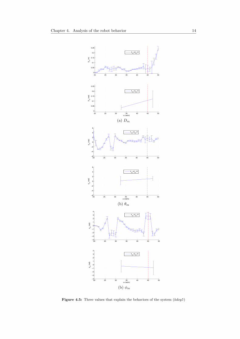
Figure 4.5: Three values that explain the behaviors of the system (kdxy5 )

15 4.3. Behavioral analysis

To characterize the behaviors further, we collect simulation results from ω = 20(rad/s)to ω = 50(rad/s) for 10(s) each and calculated the values of ~pi, ~qi (i = 0, · · · , 5)in equation (3.1) and (3.2), where t0 = 5(s) and t5 = 10(s). Also, we get ~pm, ~qmdefined in equation (3.3) along with σDm, σθm, σφm, which are standard deviationsfor Di, θi, φi (i = 1, · · · , 5), respectively. Figure 4.5 and 4.6 show the graphs ofDm, θm, φm with their standard deviations along ω = 20 ∼ 50(rad/s), in differentenvironments (top). Additionally, we calculated combined means and combinedvariances for each value, with respect to each environment’s behavioral frequencyrange. Note that the data of the range ω = 0 ∼ 20 (rad/s) are omitted here interms of the data’s usefulness.

Firstly, we focus on the graphs of kdxy5 (Figure 4.5). In the plot of Dm, it canbe noticed that the value tends to dramatically increase in higher frequency range(ω = 45 ∼ 50(rad/s)), while in the other lower frequency range the value fluctuatesaround 0.03(m). we also can see that the standard deviation σDm goes also higherwhile ω increasing, which will not affect the performance for reach-the-goal schemeso much at this frequency range, although may have something to do with thestability of locomotion. As for θm, it is shown that in low frequency range (ω = 20 ∼45(rad/s)), the combined variance of σθm is larger than that of higher frequencyrange (ω = 45 ∼ 50(rad/s)). This means the direction of the movement is relativelystraight in the high frequency range, and curvy in the low frequency range, whichcan be seen by the examples in Figure 4.3(b). Observing the graphs of φm, however,no distinct difference between the two frequency range can be found, which meansthe change of the robot’s orientation does not depend on specific frequency range.

Chapter 4. Analysis of the robot behavior 16

20 25 30 35 40 45 50

0

0.05

0.1

0.15

0.2

0.25

Dm

(m)

kxy

=dxy

=10

20 25 30 35 40 45 50

0

0.05

0.1

0.15

0.2

0.25

ω (rad/s)

Dm

(ra

d)

kxy

=dxy

=10

(a) Dm

20 25 30 35 40 45 50−6

−4

−2

0

2

4

6

θm

(ra

d)

kxy

=dxy

=10

20 25 30 35 40 45 50−6

−4

−2

0

2

4

6

ω (rad/s)

θm

(ra

d)

kxy

=dxy

=10

(b) θm

20 25 30 35 40 45 50−4

−3

−2

−1

0

1

2

3

4

φm

(ra

d)

kxy

=dxy

=10

20 25 30 35 40 45 50−4

−3

−2

−1

0

1

2

3

4

ω (rad/s)

φm

(ra

d)

kxy

=dxy

=10

(c) φm

Figure 4.6: Three values that explain the behaviors of the system (kdxy10 )

17 4.3. Behavioral analysis

The results of the analysis are almost same in the case of kdxy10 , except for thelocation of the boundary line between the frequency ranges. Dm tends to go higherat the frequency between ω = 35(rad/s) and ω = 50(rad/s). θm also slightly in-creases in this range of frequency, but σθm decreases. It can therefore be seen that inkdxy10 the displacement magnitude Dm, or absolute velocity within 1(s), increasesas the frequency goes high, while the standard deviation of the displacement angletends to decrease. Note that we cannot collect proper data if the frequency getseven higher than 50(rad/s). In that frequency range, Dm becomes even larger andmore unstable (σDm goes higher) so that the robot falls over after some period oftime, the head point hitting the ground. This unstable characteristic of the robotin the frequency range higher than ω = 50(rad/s) is also be seen in kdxy5 .

By observing Figure 4.3 to Figure 4.6, we can find two distinguished behaviorsin different frequency range, which are meaningful to the reach-the-goal scheme.Some references also use the term behavioral primitive as an unit of behavior abovethe level of motor commands which can be used as building blocks to generatemore complex movement [28,29]. Ignoring the frequency range when the robot canbarely move, i.e. approximately 0 ∼ 20(rad/s), the two different behavioral typesshown by Figure 4.3 to Figure 4.6 can be described as follows, for the behaviorsin each environment: in kdxy5 , the robot is apt to change its direction in lowfrequency range (ω = 20 ∼ 45(rad/s)), while tends to keeps its direction in higherone (ω = 45 ∼ 50(rad/s)); as for kdxy10 , the tendency is quite similar to the caseof kdxy5 , because the robot also tends to change direction with low displacementamplitude in low frequency range (ω = 20 ∼ 35(rad/s)), while relatively movestraight with high speed in higher frequency range (ω = 35 ∼ 50(rad/s)). In thenext section, it will be shown that by using ASM, it is possible to take advantageof these two behavioral types which characterize the mechanical dynamics of therobot, such that the robot is able to perform goal-directed locomotion, namely,reach-the-goal scheme.

Chapter 5

Goal-directed multi-modallocomotion

As Attractor Selection Mechanism (ASM) and mechanical dynamics of the CurvedBeam Hopping Robot are described in previous chapters, this chapter will be abouthow a goal-directed multi-modal locomotion can be realized by coupling the me-chanical dynamics with the dynamics of ASM. The next two sections will illustratethe setting of the simulation experiment of the reach-the-goal-scheme, and show theconsequential experimental results.

5.1 Experimental setting

The most important setting in the reach-the-goal experiment is the coupling betweenthe mechanical dynamics of the robot and the dynamics of ASM, as described inequation (2.1). By using only ω(t) as the control parameter, the coupling can berepresented more specifically as:

ω = −∇U(ω(t))A(t) + ε(t) (5.1)

U(ω(t)) = (ω(t)− ω1)2(ω(t)− ω2)2 (5.2)

A(t) =k

d(t)(5.3)

where U(ω(t)) is potential which composed of two frequency attractor ω1 and ω2.A(t) is sensory feedback function, which components are k = 1 and d(t). d(t) isdefined as the distance between the goal point and the curved beam’s connectionpoint to the base. Note that although in theory if the robot get to the goal point sothat d(t) = 0, A(t) becomes infinity, in numerical experiment (and supposedly alsoin real world experiment) it is almost impossible for d(t) to be exactly 0, so thatthe system keeps A(t) <∞. To avoid any obscurity of expression in the theory, onecan add infinitesimally small value to the denominator, which may not affect theresult of simulation.

As can be seen from (5.2) and Figure 5.1, U(ω(t)) is a fourth-order equation withtwo attractors, which is different depending on the environment. By choosing theseattractors according to the environment, it is assumed that the motor frequency,ω(t), will adequately fluctuate between the two meaningful frequency ranges, allow-ing the robot to explore the different behavioral types. If A(t) keeps large value,which means the goal is close, the robot tends to stick with current behavior. On

18

19 5.1. Experimental setting

20 25 30 35 40 45 500

500

1000

1500

2000

2500

3000

ω=motor frequency(rad/s)

U(ω

(t))

A(t

)

A(t)=1.4

A(t)=0.7

A(t)=0.35

(a) kdxy5

20 25 30 35 40 45 500

500

1000

1500

2000

2500

3000

ω=motor frequency(rad/s)

U(ω

(t))

A(t

)

A(t)=1.4

A(t)=0.7

A(t)=0.35

(b) kdxy10

Figure 5.1: The potential function U(ω(t)) in each environment

the other hand, if the distance from the goal point is large enough, system becomesmore stochastic because of small A(t), so that the robot tends to change its direc-tion. The robot does not have information about its orientation based on the goalpoint, and neither does about its own behavior. As a result, the resilience to changesin the operating environment, one of the fundamental properties of self-organizingsystem, is maintained. However, as will be shown in the next section, it is necessaryfor the robot to be able to explore the two different behavioral types to reach thegoal.

In a 250-second-simulation , the robot starts from the point of (x, y) = (0, 0) with itsforefoot facing to the positive x direction, and the goal point is (x, y) = (1, 1). Notethat the coordinate setting is based on the absolute Cartesian coordinate. In orderto avoid inefficiency caused by the complexity of the simulation, SimmechanicsTM

automatically vary the sampling time, with an average of approximately 0.05(s).The condition of the potential at the initial distance is shown in Figure 5.1, i.e.A(t) = 0.7. The other two cases in the figure illustrate the conditions when thedistance has half the value or a double of the initial condition.

Since the system used in the goal-directed scheme basically should be stochasticone, 10 trials for each setting out of 20 settings have conducted. More specifically,changeable factors of the setting are: kx = ky = dx = dy = 5 or 10 in GCM forthe environmental settings; two attractor arrangements−ω1 = 42.5(rad/s), ω2 =47.5(rad/s) and ω1 = 27.5(rad/s), ω2 = 42.5(rad/s)−for initial angular frequencyof rotating object; σ(ε(t)) = 0, 50, 100, 150, 200, the standard variation of internalnoise, which will be referred as level of noise. Note that, however, only 1 trial hasbeen conducted in the case of σ(ε(t)) = 0 because with this setting the system isdeterministic. For some noise settings, the result is omitted or presented withoutany figure, because of its obviousness.

The reader should also be informed that there are largely two experiments depend-ing on the experimental settings mentioned above: the first experiment is 250-second-simulation with only one attractor arrangement, i.e. ω1 = 27.5(rad/s), ω2 =42.5(rad/s), in two different environment with all level of noise; the second experimentis also 250-second-simulation with proper attractor arrangement for each environ-ment with all level of noise. That is, in this experiment the arrangement ω1 =

Chapter 5. Goal-directed multi-modal locomotion 20

42.5(rad/s), ω2 = 47.5(rad/s) is implemented for kdxy5 , and ω1 = 27.5(rad/s), ω2 =42.5(rad/s) for kdxy10 .

5.2 Experiment results

According to the interplay among the potential function of ASM which changes inshape due to A(t), a correct level of noise ε(t), and the mechanical dynamics, it isassumed that ω(t) will adequately fluctuate so that the robot takes advantage ofdifferent attractors which correspond to the different locomotion modes describedin Chapter 4. When the robot closes to the goal, A(t) gets higher, which shouldlet the robot have tendency to keep the current locomotion mode which bring ittowards the goal, without the necessity to know the detail of the behaviors.

21 5.2. Experiment results

(a) kdxy5 (left) kdxy10 (right) when σ(ε(t)) = 100

(b) kdxy5 (left) kdxy10 (right) when σ(ε(t)) = 150

Figure 5.2: Frequency fluctuations and trajectories in different conditions

Chapter 5. Goal-directed multi-modal locomotion 22

Figure 5.2 and 5.4 shows the results of the first experiment. In Figure 5.2, therobot behaviors for different levels of noise in kdxy5, and kdxy10 are shown. In5.4, The performance of the robot in the two environments with fixed attractorarrangement(ω1 = 27.5(rad/s), ω2 = 42.5(rad/s)) is shown by the blue dashed andthe red line respectively. In Figure 5.2, it can be seen that for an appropriate levelof noise, σ(ω(t)) = 150, the robot may adequately explore the different attrac-tors which bring it towards the goal. However, when the level of noise is too lowσ(ω(t)) = 100, it is difficult for the robot to explore different attractors. On theother hand, when the level of noise is too large, the frequency can reach high valueswhere the robot to can become unstable, which reduces the performance, or makethe robot fall over. It can therefore be understood that Figure 5.4 shows that thebest performance of the robot is achieved with the level of noise σ(ω(t)) = 150. Ifwe focus on the result of kdxy5, it is important to notice that both attractors aredifferent from those introduced in Chapter 4. Therefore, in kdxy5, with the sameattractor arrangement as in kdxy10, the robot shows less distinguishable behaviorsof keep moving forward or change direction than those in kdxy10.

23 5.2. Experiment results

Figure 5.3: Frequency fluctuations and trajectories in kdxy5 when σ(ε(t)) = 50 (left),and those in kdxy10 when σ(ε(t)) = 150 (right) respectively

Figure 5.4: Performance of numerical experiments with various levels of noise

In the second experiment, we additionally observe the behavior of the robot inkdxy5 when the attractors are corrected to be ω1 = 42.5 and ω2 = 47.5 (rad/s),as shown in Figure 5.1 or as defined in Chapter 4. Here, the important differencefrom the first experiment is that for kdxy5, the new attractor arrangement makethe robot has go-straight locomotion mode at ω = 47.5(rad/s). We can confirmin Figure 5.3 that Having two distinct locomotion modes in kdxy5, the robot canreach the goal point accurately (in terms of minimal distance). If we have a look onthe average minimal distance in Figure 5.4, it is also interesting to notice that thelevel of noise which leads to the best performance is σ(ω(t)) = 50, which is lowerthan the best level in the first experiment. It is further confirmed in the figurethat in the same environment, i.e. kdxy5, the average of minimum distance reachedby the robot with the second arrangement of attractors is lower compared to thatwith the first arrangement. This result is understandable in the context of proper

Chapter 5. Goal-directed multi-modal locomotion 24

coupling between ASM and the mechanical dynamics of the robot. In the secondexperiment, we can recognize the robot can reach the goal point closer comparedto the first experiment due to the ability to travel in go-straight way, which meansthe rearranged ASM attractors are coupled better, with the mechanical dynamics,than the previous experiment.

Chapter 6

Real-world experiment

Having confirmed the validity of the used approach in numerical experiments, weexamined the same principle on real-world robot. First, we investigate the behav-ioral property of the robot by using FFT. Then, with similar experimental settings,we demonstrate the result of real-world experiments with different noise level. Notethat all the real-world experiments are conducted by Xiaoxiang Yu, who is now analumni of BIRLab.

6.1 Behavioral analysis

Figure 6.1: The dominant amplitudes of head point’s oscillation

For getting knowledge of the real robot’s behavioral characteristics, we calculatedFFT on the behaviors of the robot at each rotating frequency, by using motion cap-ture system. Figure 6.1 shows the dominant amplitudes of robot head’s oscillation.Due to the hardware limitation, The frequency range in the real robot is limited toapproximately 20[rad/s], corresponds roughly to 5[V] for the DC motor. Becauseof the interactions with real world environment, the oscillations of the head pointcan be different in each trial. We therefore perform five trials and plot the averageand standard deviation in Figure 6.1. It can be observed that despite the frequencyrange is different with the simulation, at higher frequencies, the amplitude at the xdirection also becomes higher than those along z direction. However, the amplitudesat the y direction are significantly smaller than those at x direction.

25

Chapter 6. Real-world experiment 26

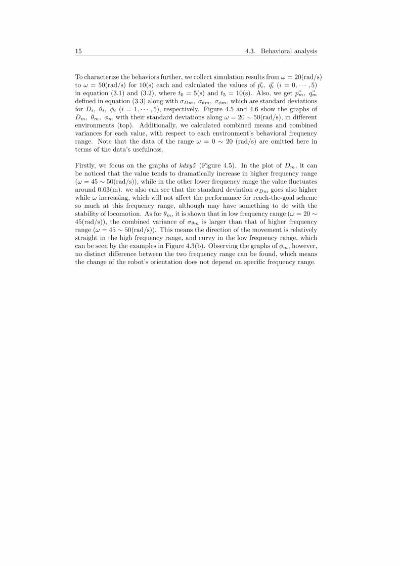
Figure 6.2: The dominant amplitudes of head point’s oscillation

To understand how it affects the behavior of the robot, we plot several trajectoryexamples at different values of rotating frequency (ω = 13[rad/s] on the left, andω = 17[rad/s] on the right) as shown in Figure 6.2. We have also noticed that anincreasing number of segments in the simulation causes the mechanical dynamics tobecome more similar with the real world robot, but also increases the computationtime significantly.

6.2 Experimental setting

The rotating frequency of the real robot is controlled through the voltage of theDC motor attached to the head part. We therefore define the attractors for ASMin voltage unit as V1 = 3.2[V] and V2 = 3.9[V], which roughly corresponds toω1 = 13[rad/s] and ω = 17[rad/s], respectively. Accordingly, equation 5.1, 5.2, 5.3are applied to the real robot with different form:

V = −∇U(V (t))AV (t) + εV (t) (6.1)

U(V (t)) = (V (t)− V1)2(V (t)− V2)2 (6.2)

AV (t) =k

d(t)(6.3)

where k = 1.

27 6.3. Experiment results

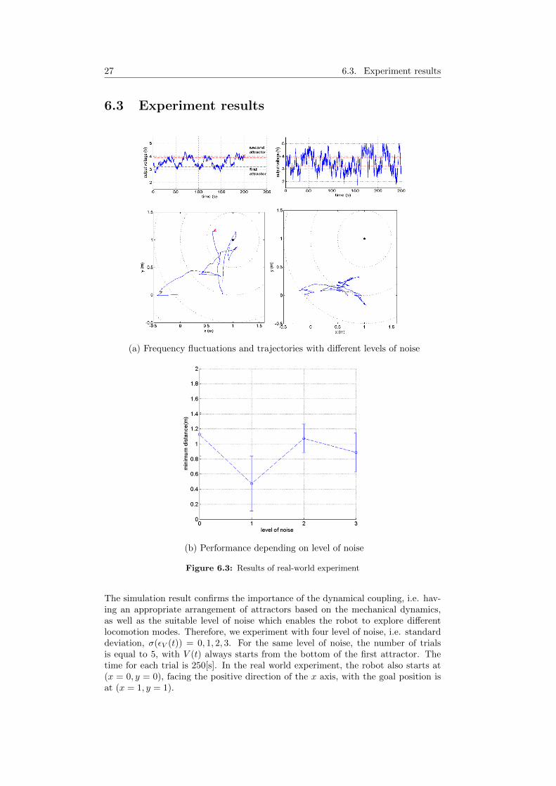
6.3 Experiment results

(a) Frequency fluctuations and trajectories with different levels of noise

(b) Performance depending on level of noise

Figure 6.3: Results of real-world experiment

The simulation result confirms the importance of the dynamical coupling, i.e. hav-ing an appropriate arrangement of attractors based on the mechanical dynamics,as well as the suitable level of noise which enables the robot to explore differentlocomotion modes. Therefore, we experiment with four level of noise, i.e. standarddeviation, σ(εV (t)) = 0, 1, 2, 3. For the same level of noise, the number of trialsis equal to 5, with V (t) always starts from the bottom of the first attractor. Thetime for each trial is 250[s]. In the real world experiment, the robot also starts at(x = 0, y = 0), facing the positive direction of the x axis, with the goal position isat (x = 1, y = 1).

Chapter 6. Real-world experiment 28

The trajectory examples for different levels of noise, as well as the performance, areshown in Figure 6.3 (a) and (b). From the graphs on the left in Figure 6.3 (a), it canbe seen that due to the coupling between the mechanical dynamics and the ASMdynamics, the robot can adequately explore different locomotion modes through theinterplay among the changing potential function and an appropriate level of noise,i.e. σ(εV (t)) = 1. On the other hand, the graphs on the right in Figure 6.3 (a) showsthe case when the level of noise is too high, σ(εV (t)) = 3, causing the fluctuation offrequency becomes almost entirely random that fails to bring the robot towards thegoal. These are can be re-confirmed by paying attention to Figure 6.3 (b), whichshows overall performance on multiple experiments.

Chapter 7

Conclusion

We have shown that by using proposed methods complex model like Curved BeamHopping Robot can achieve goal-directed locomotion in different environmental set-tings using two distinct locomotion modes, which shows us its multi-modality. Bycoupling the mechanical dynamics and the controller, Attractor Selection Mecha-nism, it was possible for the robot to take advantage of the different locomotionmodes to bring itself towards the goal point. We showed this through the simu-lation and real-world experiment. If the sensory input indicates that the robot isapproaching the goal point, the robot will behave more deterministically, keepingits current behavior. Otherwise, when the robot is far from the goal point, it willbehave rather stochastically, searching proper attractor which brings it closer to thegoal. Even in different environment, the robot can still reach the goal as long as themechanical dynamics is correlated to the ASM dynamics. In spite of the simplicityof the approach, the results let us confirm that dynamical coupling is important toachieve goal-directed locomotion.

In principle, an approach proposed in this thesis is to achieve goal-directed behaviorby knowing only a limited knowledge about the robot dynamics. The approach re-lies on different emerging modes without detailed knowledge of the mechanism thatcreates them. It is also interesting to notice that the described behavior is createdbased on the mechanism used by simple creatures which do not even have a neuralmechanism. While there are the studies which focus on achieving similar behaviorby using chaotic dynamics [2,30,31,33], the approach described in this thesis relieson stochastic dynamics and can lead to a different perspective on how to achievegoal-directed locomotion with embodied system.

The approach explained in this thesis emphasizes the importance of interactionsamong internal control structure, physical body and environment. From the per-spective of morphological computation concept [14, 15, 32], it can also be said thatthe interactions between the mechanical body of robot and the environment giverise to particular body-environment attractors, which simplify the control processif the mechanical and the controller dynamics are properly coupled.

For future work, simulation studies based on more realistic environmental changeshould be considered. Since the locomotion primitives of the robot diverse alsodepending on the environment(GCM, in this case), it will undergird the multi-modality of the robotic platform like the one used in this thesis. Furthermore, itwill also be interesting approach to change morphological structure of Curved BeamHopping Robot, so that we can find other new meaningful behaviors of the robot forvarious tasks. Finally, in this thesis, the proper coupling between internal control

29

Chapter 7. Conclusion 30

structure, i.e. ASM, and the mechanical dynamics is still designed manually. Asa future work concerning this aspect, how the coupling can be adjusted in on-linemanner should be investigated.

Bibliography

[1] Lock R. J., Burgess S. C. and Vaidyanathan R., “Multi modal locomotion:from animal to application,” Bioinspir. Biomim., 9 : 1-18, 2014

[2] Auke J. I., Crespi A., Ryczko D. and Cabelguen J. M., “From Swimming toWalking with a Salamander Robot Driven by a Spinal Cord Model,” Science,515(5817) : 1416-1420, 2007

[3] Nudds R. L., Folkow L. P., Lees J. J., Tickle P. G., Stokkan K. and CoddJ. R., “Evidence for energy savings from aerial running in the Svalbard rockptarmigan (Lagopus muta hyperborea),” Proc. Biol. Sci. /R. Soc., 278: 2654-61, 2011

[4] Emerson S. B., “The interaction of behavioral and morphological change in theevolution of a novel locomotor mode: ′flying′ frogs,” Evolution, 44 : 1931-46,1990

[5] Hosoda K., Takuma T., Nakamoto A. and Hayashi S., “Biped robot designpowered by antagonistic pneumatic actuators for multi-modal locomotion,”Robot. Auton. Syst., 56(1) : 46-53, 2008

[6] Iida F., Rummel J. and Seyfarth A., “Bipedal walking and running with com-pliant legs,” IEEE Int. Conf. on Robotics and Automation (ICRA2007), pp.3970-3975, 2007

[7] Sayyad A., Seth B. and Seshu P., “Single-legged hopping robotics research - areview,” Robotica, 25 : 587-613, 2007

[8] Berkemier M. D. and Fearing R. S., “Sliding and hopping gaits for the under-actuated acrobot,” IEEE T. Robotics. Autom., 14(4) : 629-634, 1998

[9] Nurzaman S. G., Matsumoto Y., Nakamura Y., Shirai K., Koizumi S. and Ishig-uro H., “From Levy to Brownian: A computational model based on biologicalfluctuation,” PLoS ONE, 6(2) : e16168, 2010

[10] Pfeifer R., Lungarella M. and Iida F., “Self organization, embodiment andbiologically inspired robotics,” Science, 318(5853) : 1088-1093, 2007

[11] Hoffmann, M. and Pfeifer R., “The implications of embodiment for behav-ior and cognition: animal and robotic case studies. In The Implications ofEmbodiment: Cognition and Communication,” W. Tschacher & C. Bergomi(ed.), Exeter : Imprint Academic, pp. 31-58

[12] Rieffel J., Valero-Cuevas F. and Lipson H., “Morphological communication:exploiting coupled dynamics in a complex mechanical structure to achieve lo-comotion,” J. R. Soc. Interface, 7(45) : 613-621, 2009

31

Bibliography 32

[13] Khazanov M., Humphreys B., Keat W. and Rieffel J., “Exploiting dynamicalcomplexity in a physical tensegrity robot to achieve locomotion,” Advances inArtificial Life (ECAL 2013), pp. 965-972, 2013

[14] Fuechslin R. M., Dzyakanchuk A., Hauser H., Hunt, K. J., Luchsinger R. H.,Reller, B. L., Scheidegger S., Walkter R., Scheidegger S. and Walker R., “Mor-phological computation and morphological control : steps toward a formal the-ory and applications,” Artificial Life, 19 : 9-34, 2013

[15] Iida F. and Preifer R., “Sensing through body dynamics,” Robotics and Au-tonomous Systems, 54 : 631-640, 2006

[16] Yanagida T., Ueda M., Murata T., Esaki S. and Ishii Y., “Brownian motion,fluctuation and life,” BioSystems, 88 : 228-242, 2007

[17] Kashiwagi A., Ureba I., Kaneko K. and Yomo T., “Adaptive response of agene network to environmental changes by fitness-induced attractor selection,”PLoS ONE, 1(1) : e49, 2006

[18] Nurzaman S. G., Matsumoto Y., Nakamura Y., Shirai K. and Ishiguro H.,“Bacteria-inspired underactuated mobile robot based on a biological fluctua-tion,” Adaptive Behavior, 20(4) : 225-236, 2012

[19] Nurzaman S. G., Matsumoto Y., Nakamura Y., Koizumi S. and IshiguroH., “”Yuragi”-based adaptive mobile robot search with and without gradi-ent sensing: from bacterial chemotaxis to a Levy walk,” Advanced Robotics,25(16) : 2019-2037, 2011

[20] Nurzaman S. G., Matsumoto Y., Nakamura Y., Koizumi S. and Ishiguro H.,“Attractor selection based biologically inspired navigation system,” Proceedingsof the 39th International Symposium on Robotics, pp. 837-842, 2008

[21] Reis M. and Iida F., “An energy efficient hopping robot based on a free vibra-tion of a curved beam,” IEEE/ASME Trans. Mechatronics, 19(1) : 300-311,2013

[22] Yu X. and Iida F., “Minimalistic models of an energy-efficient vertical-hoppingrobot,” IEEE Trans. Ind. Electron, 61(2) : 1035-1062, 2013

[23] Prokopenko M, “Design vs Self-organization. In Advances in Applied Self-organizing Systems,” M. Prokopenko (ed.), Springer-Verlag, London, UK, pp.3-17, 2007

[24] Martius G. and Herrmann J. M., “Variants of guided self-organization for robotcontrol Theory,”Biosci., 131: 129-137, 2012

[25] Hesse F., Martius G. J. M., Der R. and Herrmann J. M., “A sensor-basedlearning algorithm for the self organization of robot behavior,” Algorithms 2:398-409, 2009

[26] MathWorks Official Homepage: http: //www.mathworks.com/products/simmechanics/ (accessed on March 27th, 2014).

[27] Brubaker M. A., Sigal L. and Fleet D. J., “Estimating contact dynamics,”Proceedings of the IEEE International Conference on Computer Vision, 2389-2396, 2009

[28] Bentivegna, D., Cheng G. and Atkeson C., “Learning from observation andfrom practice using behavioral primitives,” In Springer Tracts in AdvancedRobotics, pp. 551-560, 2005

33 Bibliography

[29] Jenkins O. C. and Mataric M. J., “Deriving action and behavior primitives fromhuman motion data,” Proceedings of the IEEE/RSJ International Conferenceon Intelligent Robots and Systems, 2551-2556, 2002

[30] Santos C. P. and Matos V., “CPG modulation for navigation and omnidirec-tional quarduped locomotion,” Robotics and Autonomous Systems, 60 : 912-927, 2012

[31] Grillner S., Wallen P., Saitoh K., Kozlov A. and Robertson B., “Neural bases ofgoal-directed locomotion in vertebrates–an overview,” Brain Research Reviews,57 : 2-12, 2008

[32] Nurzaman S. G., Culha U., Brodbeck L., Wang L. and Iida F., “Active sensingsystem with in situ adjustable sensor morphology,” PLoS ONE, 8(12) : e84090,2013

[33] Shim Y. and Husbands P., “Chaotic exploration and learning of locomotionbehaviors,” Neural Computation, 24 : 2185-2222, 2012

[34] De Jager M., Weissing F. J., Herman P. M. J., Nolet B. A. and van de KoppelJ., “Levy Walks Evolve Through Interaction Between Movement and Environ-mental Complexity,” Science, 332(6037) : 1551-1553

Bibliography 34

Statement of authorship

I declare that I completed this thesis on my own and that information which hasbeen directly or indirectly taken from other sources has been noted as such. Neitherthis nor a similar work has been presented to an examination committee.

Zurich, June 27, 2014 . . . . . . . . . . . . . . . . . . . . . . . .

35