Going deeper with convolutions

Christian SzegedyGoogle Inc.

Wei LiuUniversity of North Carolina, Chapel Hill

Yangqing JiaGoogle Inc.

Pierre SermanetGoogle Inc.

Scott ReedUniversity of Michigan

Dragomir AnguelovGoogle Inc.

Dumitru ErhanGoogle Inc.

Vincent VanhouckeGoogle Inc.

Andrew RabinovichGoogle Inc.

Abstract

We propose a deep convolutional neural network architecture codenamed Incep-tion, which was responsible for setting the new state of the art for classificationand detection in the ImageNet Large-Scale Visual Recognition Challenge 2014(ILSVRC14). The main hallmark of this architecture is the improved utilizationof the computing resources inside the network. This was achieved by a carefullycrafted design that allows for increasing the depth and width of the network whilekeeping the computational budget constant. To optimize quality, the architecturaldecisions were based on the Hebbian principle and the intuition of multi-scaleprocessing. One particular incarnation used in our submission for ILSVRC14 iscalled GoogLeNet, a 22 layers deep network, the quality of which is assessed inthe context of classification and detection.

1 Introduction

In the last three years, mainly due to the advances of deep learning, more concretely convolutionalnetworks [10], the quality of image recognition and object detection has been progressing at a dra-matic pace. One encouraging news is that most of this progress is not just the result of more powerfulhardware, larger datasets and bigger models, but mainly a consequence of new ideas, algorithms andimproved network architectures. No new data sources were used, for example, by the top entries inthe ILSVRC 2014 competition besides the classification dataset of the same competition for detec-tion purposes. Our GoogLeNet submission to ILSVRC 2014 actually uses 12× fewer parametersthan the winning architecture of Krizhevsky et al [9] from two years ago, while being significantlymore accurate. The biggest gains in object-detection have not come from the utilization of deepnetworks alone or bigger models, but from the synergy of deep architectures and classical computervision, like the R-CNN algorithm by Girshick et al [6].

Another notable factor is that with the ongoing traction of mobile and embedded computing, theefficiency of our algorithms – especially their power and memory use – gains importance. It isnoteworthy that the considerations leading to the design of the deep architecture presented in thispaper included this factor rather than having a sheer fixation on accuracy numbers. For most of theexperiments, the models were designed to keep a computational budget of 1.5 billion multiply-addsat inference time, so that the they do not end up to be a purely academic curiosity, but could be putto real world use, even on large datasets, at a reasonable cost.

1

arX

iv:1

409.

4842

v1 [

cs.C

V]

17

Sep

2014

In this paper, we will focus on an efficient deep neural network architecture for computer vision,codenamed Inception, which derives its name from the Network in network paper by Lin et al [12]in conjunction with the famous “we need to go deeper” internet meme [1]. In our case, the word“deep” is used in two different meanings: first of all, in the sense that we introduce a new level oforganization in the form of the “Inception module” and also in the more direct sense of increasednetwork depth. In general, one can view the Inception model as a logical culmination of [12]while taking inspiration and guidance from the theoretical work by Arora et al [2]. The benefitsof the architecture are experimentally verified on the ILSVRC 2014 classification and detectionchallenges, on which it significantly outperforms the current state of the art.

2 Related Work

Starting with LeNet-5 [10], convolutional neural networks (CNN) have typically had a standardstructure – stacked convolutional layers (optionally followed by contrast normalization and max-pooling) are followed by one or more fully-connected layers. Variants of this basic design areprevalent in the image classification literature and have yielded the best results to-date on MNIST,CIFAR and most notably on the ImageNet classification challenge [9, 21]. For larger datasets suchas Imagenet, the recent trend has been to increase the number of layers [12] and layer size [21, 14],while using dropout [7] to address the problem of overfitting.

Despite concerns that max-pooling layers result in loss of accurate spatial information, the sameconvolutional network architecture as [9] has also been successfully employed for localization [9,14], object detection [6, 14, 18, 5] and human pose estimation [19]. Inspired by a neurosciencemodel of the primate visual cortex, Serre et al. [15] use a series of fixed Gabor filters of different sizesin order to handle multiple scales, similarly to the Inception model. However, contrary to the fixed2-layer deep model of [15], all filters in the Inception model are learned. Furthermore, Inceptionlayers are repeated many times, leading to a 22-layer deep model in the case of the GoogLeNetmodel.

Network-in-Network is an approach proposed by Lin et al. [12] in order to increase the representa-tional power of neural networks. When applied to convolutional layers, the method could be viewedas additional 1×1 convolutional layers followed typically by the rectified linear activation [9]. Thisenables it to be easily integrated in the current CNN pipelines. We use this approach heavily in ourarchitecture. However, in our setting, 1 × 1 convolutions have dual purpose: most critically, theyare used mainly as dimension reduction modules to remove computational bottlenecks, that wouldotherwise limit the size of our networks. This allows for not just increasing the depth, but also thewidth of our networks without significant performance penalty.

The current leading approach for object detection is the Regions with Convolutional Neural Net-works (R-CNN) proposed by Girshick et al. [6]. R-CNN decomposes the overall detection probleminto two subproblems: to first utilize low-level cues such as color and superpixel consistency forpotential object proposals in a category-agnostic fashion, and to then use CNN classifiers to identifyobject categories at those locations. Such a two stage approach leverages the accuracy of bound-ing box segmentation with low-level cues, as well as the highly powerful classification power ofstate-of-the-art CNNs. We adopted a similar pipeline in our detection submissions, but have ex-plored enhancements in both stages, such as multi-box [5] prediction for higher object boundingbox recall, and ensemble approaches for better categorization of bounding box proposals.

3 Motivation and High Level Considerations

The most straightforward way of improving the performance of deep neural networks is by increas-ing their size. This includes both increasing the depth – the number of levels – of the network and itswidth: the number of units at each level. This is as an easy and safe way of training higher qualitymodels, especially given the availability of a large amount of labeled training data. However thissimple solution comes with two major drawbacks.

Bigger size typically means a larger number of parameters, which makes the enlarged network moreprone to overfitting, especially if the number of labeled examples in the training set is limited.This can become a major bottleneck, since the creation of high quality training sets can be tricky

2

(a) Siberian husky (b) Eskimo dog

Figure 1: Two distinct classes from the 1000 classes of the ILSVRC 2014 classification challenge.

and expensive, especially if expert human raters are necessary to distinguish between fine-grainedvisual categories like those in ImageNet (even in the 1000-class ILSVRC subset) as demonstratedby Figure 1.

Another drawback of uniformly increased network size is the dramatically increased use of compu-tational resources. For example, in a deep vision network, if two convolutional layers are chained,any uniform increase in the number of their filters results in a quadratic increase of computation. Ifthe added capacity is used inefficiently (for example, if most weights end up to be close to zero),then a lot of computation is wasted. Since in practice the computational budget is always finite, anefficient distribution of computing resources is preferred to an indiscriminate increase of size, evenwhen the main objective is to increase the quality of results.

The fundamental way of solving both issues would be by ultimately moving from fully connectedto sparsely connected architectures, even inside the convolutions. Besides mimicking biologicalsystems, this would also have the advantage of firmer theoretical underpinnings due to the ground-breaking work of Arora et al. [2]. Their main result states that if the probability distribution ofthe data-set is representable by a large, very sparse deep neural network, then the optimal networktopology can be constructed layer by layer by analyzing the correlation statistics of the activationsof the last layer and clustering neurons with highly correlated outputs. Although the strict math-ematical proof requires very strong conditions, the fact that this statement resonates with the wellknown Hebbian principle – neurons that fire together, wire together – suggests that the underlyingidea is applicable even under less strict conditions, in practice.

On the downside, todays computing infrastructures are very inefficient when it comes to numericalcalculation on non-uniform sparse data structures. Even if the number of arithmetic operations isreduced by 100×, the overhead of lookups and cache misses is so dominant that switching to sparsematrices would not pay off. The gap is widened even further by the use of steadily improving,highly tuned, numerical libraries that allow for extremely fast dense matrix multiplication, exploit-ing the minute details of the underlying CPU or GPU hardware [16, 9]. Also, non-uniform sparsemodels require more sophisticated engineering and computing infrastructure. Most current visionoriented machine learning systems utilize sparsity in the spatial domain just by the virtue of em-ploying convolutions. However, convolutions are implemented as collections of dense connectionsto the patches in the earlier layer. ConvNets have traditionally used random and sparse connectiontables in the feature dimensions since [11] in order to break the symmetry and improve learning, thetrend changed back to full connections with [9] in order to better optimize parallel computing. Theuniformity of the structure and a large number of filters and greater batch size allow for utilizingefficient dense computation.

This raises the question whether there is any hope for a next, intermediate step: an architecturethat makes use of the extra sparsity, even at filter level, as suggested by the theory, but exploits our

3

current hardware by utilizing computations on dense matrices. The vast literature on sparse matrixcomputations (e.g. [3]) suggests that clustering sparse matrices into relatively dense submatricestends to give state of the art practical performance for sparse matrix multiplication. It does notseem far-fetched to think that similar methods would be utilized for the automated construction ofnon-uniform deep-learning architectures in the near future.

The Inception architecture started out as a case study of the first author for assessing the hypotheticaloutput of a sophisticated network topology construction algorithm that tries to approximate a sparsestructure implied by [2] for vision networks and covering the hypothesized outcome by dense, read-ily available components. Despite being a highly speculative undertaking, only after two iterationson the exact choice of topology, we could already see modest gains against the reference architec-ture based on [12]. After further tuning of learning rate, hyperparameters and improved trainingmethodology, we established that the resulting Inception architecture was especially useful in thecontext of localization and object detection as the base network for [6] and [5]. Interestingly, whilemost of the original architectural choices have been questioned and tested thoroughly, they turnedout to be at least locally optimal.

One must be cautious though: although the proposed architecture has become a success for computervision, it is still questionable whether its quality can be attributed to the guiding principles that havelead to its construction. Making sure would require much more thorough analysis and verification:for example, if automated tools based on the principles described below would find similar, butbetter topology for the vision networks. The most convincing proof would be if an automatedsystem would create network topologies resulting in similar gains in other domains using the samealgorithm but with very differently looking global architecture. At very least, the initial success ofthe Inception architecture yields firm motivation for exciting future work in this direction.

4 Architectural Details

The main idea of the Inception architecture is based on finding out how an optimal local sparsestructure in a convolutional vision network can be approximated and covered by readily availabledense components. Note that assuming translation invariance means that our network will be builtfrom convolutional building blocks. All we need is to find the optimal local construction and torepeat it spatially. Arora et al. [2] suggests a layer-by layer construction in which one should analyzethe correlation statistics of the last layer and cluster them into groups of units with high correlation.These clusters form the units of the next layer and are connected to the units in the previous layer. Weassume that each unit from the earlier layer corresponds to some region of the input image and theseunits are grouped into filter banks. In the lower layers (the ones close to the input) correlated unitswould concentrate in local regions. This means, we would end up with a lot of clusters concentratedin a single region and they can be covered by a layer of 1×1 convolutions in the next layer, assuggested in [12]. However, one can also expect that there will be a smaller number of morespatially spread out clusters that can be covered by convolutions over larger patches, and therewill be a decreasing number of patches over larger and larger regions. In order to avoid patch-alignment issues, current incarnations of the Inception architecture are restricted to filter sizes 1×1,3×3 and 5×5, however this decision was based more on convenience rather than necessity. It alsomeans that the suggested architecture is a combination of all those layers with their output filterbanks concatenated into a single output vector forming the input of the next stage. Additionally,since pooling operations have been essential for the success in current state of the art convolutionalnetworks, it suggests that adding an alternative parallel pooling path in each such stage should haveadditional beneficial effect, too (see Figure 2(a)).

As these “Inception modules” are stacked on top of each other, their output correlation statisticsare bound to vary: as features of higher abstraction are captured by higher layers, their spatialconcentration is expected to decrease suggesting that the ratio of 3×3 and 5×5 convolutions shouldincrease as we move to higher layers.

One big problem with the above modules, at least in this naıve form, is that even a modest number of5×5 convolutions can be prohibitively expensive on top of a convolutional layer with a large numberof filters. This problem becomes even more pronounced once pooling units are added to the mix:their number of output filters equals to the number of filters in the previous stage. The merging ofthe output of the pooling layer with the outputs of convolutional layers would lead to an inevitable

4

1x1 convolutions 3x3 convolutions 5x5 convolutions

Filter concatenation

Previous layer

3x3 max pooling

(a) Inception module, naıve version

1x1 convolutions

3x3 convolutions 5x5 convolutions

Filter concatenation

Previous layer

3x3 max pooling1x1 convolutions 1x1 convolutions

1x1 convolutions

(b) Inception module with dimension reductions

Figure 2: Inception module

increase in the number of outputs from stage to stage. Even while this architecture might cover theoptimal sparse structure, it would do it very inefficiently, leading to a computational blow up withina few stages.

This leads to the second idea of the proposed architecture: judiciously applying dimension reduc-tions and projections wherever the computational requirements would increase too much otherwise.This is based on the success of embeddings: even low dimensional embeddings might contain a lotof information about a relatively large image patch. However, embeddings represent information ina dense, compressed form and compressed information is harder to model. We would like to keepour representation sparse at most places (as required by the conditions of [2]) and compress thesignals only whenever they have to be aggregated en masse. That is, 1×1 convolutions are used tocompute reductions before the expensive 3×3 and 5×5 convolutions. Besides being used as reduc-tions, they also include the use of rectified linear activation which makes them dual-purpose. Thefinal result is depicted in Figure 2(b).

In general, an Inception network is a network consisting of modules of the above type stacked uponeach other, with occasional max-pooling layers with stride 2 to halve the resolution of the grid. Fortechnical reasons (memory efficiency during training), it seemed beneficial to start using Inceptionmodules only at higher layers while keeping the lower layers in traditional convolutional fashion.This is not strictly necessary, simply reflecting some infrastructural inefficiencies in our currentimplementation.

One of the main beneficial aspects of this architecture is that it allows for increasing the number ofunits at each stage significantly without an uncontrolled blow-up in computational complexity. Theubiquitous use of dimension reduction allows for shielding the large number of input filters of thelast stage to the next layer, first reducing their dimension before convolving over them with a largepatch size. Another practically useful aspect of this design is that it aligns with the intuition thatvisual information should be processed at various scales and then aggregated so that the next stagecan abstract features from different scales simultaneously.

The improved use of computational resources allows for increasing both the width of each stageas well as the number of stages without getting into computational difficulties. Another way toutilize the inception architecture is to create slightly inferior, but computationally cheaper versionsof it. We have found that all the included the knobs and levers allow for a controlled balancing ofcomputational resources that can result in networks that are 2− 3× faster than similarly performingnetworks with non-Inception architecture, however this requires careful manual design at this point.

5 GoogLeNet

We chose GoogLeNet as our team-name in the ILSVRC14 competition. This name is an homage toYann LeCuns pioneering LeNet 5 network [10]. We also use GoogLeNet to refer to the particularincarnation of the Inception architecture used in our submission for the competition. We have alsoused a deeper and wider Inception network, the quality of which was slightly inferior, but adding itto the ensemble seemed to improve the results marginally. We omit the details of that network, sinceour experiments have shown that the influence of the exact architectural parameters is relatively

5

typepatch size/

strideoutput

sizedepth #1×1

#3×3

reduce#3×3

#5×5

reduce#5×5

poolproj

params ops

convolution 7×7/2 112×112×64 1 2.7K 34M

max pool 3×3/2 56×56×64 0

convolution 3×3/1 56×56×192 2 64 192 112K 360M

max pool 3×3/2 28×28×192 0

inception (3a) 28×28×256 2 64 96 128 16 32 32 159K 128M

inception (3b) 28×28×480 2 128 128 192 32 96 64 380K 304M

max pool 3×3/2 14×14×480 0

inception (4a) 14×14×512 2 192 96 208 16 48 64 364K 73M

inception (4b) 14×14×512 2 160 112 224 24 64 64 437K 88M

inception (4c) 14×14×512 2 128 128 256 24 64 64 463K 100M

inception (4d) 14×14×528 2 112 144 288 32 64 64 580K 119M

inception (4e) 14×14×832 2 256 160 320 32 128 128 840K 170M

max pool 3×3/2 7×7×832 0

inception (5a) 7×7×832 2 256 160 320 32 128 128 1072K 54M

inception (5b) 7×7×1024 2 384 192 384 48 128 128 1388K 71M

avg pool 7×7/1 1×1×1024 0

dropout (40%) 1×1×1024 0

linear 1×1×1000 1 1000K 1M

softmax 1×1×1000 0

Table 1: GoogLeNet incarnation of the Inception architecture

minor. Here, the most successful particular instance (named GoogLeNet) is described in Table 1 fordemonstrational purposes. The exact same topology (trained with different sampling methods) wasused for 6 out of the 7 models in our ensemble.

All the convolutions, including those inside the Inception modules, use rectified linear activation.The size of the receptive field in our network is 224×224 taking RGB color channels with mean sub-traction. “#3×3 reduce” and “#5×5 reduce” stands for the number of 1×1 filters in the reductionlayer used before the 3×3 and 5×5 convolutions. One can see the number of 1×1 filters in the pro-jection layer after the built-in max-pooling in the pool proj column. All these reduction/projectionlayers use rectified linear activation as well.

The network was designed with computational efficiency and practicality in mind, so that inferencecan be run on individual devices including even those with limited computational resources, espe-cially with low-memory footprint. The network is 22 layers deep when counting only layers withparameters (or 27 layers if we also count pooling). The overall number of layers (independent build-ing blocks) used for the construction of the network is about 100. However this number depends onthe machine learning infrastructure system used. The use of average pooling before the classifier isbased on [12], although our implementation differs in that we use an extra linear layer. This enablesadapting and fine-tuning our networks for other label sets easily, but it is mostly convenience andwe do not expect it to have a major effect. It was found that a move from fully connected layers toaverage pooling improved the top-1 accuracy by about 0.6%, however the use of dropout remainedessential even after removing the fully connected layers.

Given the relatively large depth of the network, the ability to propagate gradients back through all thelayers in an effective manner was a concern. One interesting insight is that the strong performanceof relatively shallower networks on this task suggests that the features produced by the layers in themiddle of the network should be very discriminative. By adding auxiliary classifiers connected tothese intermediate layers, we would expect to encourage discrimination in the lower stages in theclassifier, increase the gradient signal that gets propagated back, and provide additional regulariza-tion. These classifiers take the form of smaller convolutional networks put on top of the output ofthe Inception (4a) and (4d) modules. During training, their loss gets added to the total loss of thenetwork with a discount weight (the losses of the auxiliary classifiers were weighted by 0.3). Atinference time, these auxiliary networks are discarded.

The exact structure of the extra network on the side, including the auxiliary classifier, is as follows:

• An average pooling layer with 5×5 filter size and stride 3, resulting in an 4×4×512 outputfor the (4a), and 4×4×528 for the (4d) stage.

6

input

Conv7x7+2(S)

MaxPool3x3+2(S)

LocalRespNorm

Conv1x1+1(V)

Conv3x3+1(S)

LocalRespNorm

MaxPool3x3+2(S)

Conv1x1+1(S)

Conv1x1+1(S)

Conv1x1+1(S)

MaxPool3x3+1(S)

DepthConcat

Conv3x3+1(S)

Conv5x5+1(S)

Conv1x1+1(S)

Conv1x1+1(S)

Conv1x1+1(S)

Conv1x1+1(S)

MaxPool3x3+1(S)

DepthConcat

Conv3x3+1(S)

Conv5x5+1(S)

Conv1x1+1(S)

MaxPool3x3+2(S)

Conv1x1+1(S)

Conv1x1+1(S)

Conv1x1+1(S)

MaxPool3x3+1(S)

DepthConcat

Conv3x3+1(S)

Conv5x5+1(S)

Conv1x1+1(S)

Conv1x1+1(S)

Conv1x1+1(S)

Conv1x1+1(S)

MaxPool3x3+1(S)

AveragePool5x5+3(V)

DepthConcat

Conv3x3+1(S)

Conv5x5+1(S)

Conv1x1+1(S)

Conv1x1+1(S)

Conv1x1+1(S)

Conv1x1+1(S)

MaxPool3x3+1(S)

DepthConcat

Conv3x3+1(S)

Conv5x5+1(S)

Conv1x1+1(S)

Conv1x1+1(S)

Conv1x1+1(S)

Conv1x1+1(S)

MaxPool3x3+1(S)

DepthConcat

Conv3x3+1(S)

Conv5x5+1(S)

Conv1x1+1(S)

Conv1x1+1(S)

Conv1x1+1(S)

Conv1x1+1(S)

MaxPool3x3+1(S)

AveragePool5x5+3(V)

DepthConcat

Conv3x3+1(S)

Conv5x5+1(S)

Conv1x1+1(S)

MaxPool3x3+2(S)

Conv1x1+1(S)

Conv1x1+1(S)

Conv1x1+1(S)

MaxPool3x3+1(S)

DepthConcat

Conv3x3+1(S)

Conv5x5+1(S)

Conv1x1+1(S)

Conv1x1+1(S)

Conv1x1+1(S)

Conv1x1+1(S)

MaxPool3x3+1(S)

DepthConcat

Conv3x3+1(S)

Conv5x5+1(S)

Conv1x1+1(S)

AveragePool7x7+1(V)

FC

Conv1x1+1(S)

FC

FC

SoftmaxActivation

softmax0

Conv1x1+1(S)

FC

FC

SoftmaxActivation

softmax1

SoftmaxActivation

softmax2

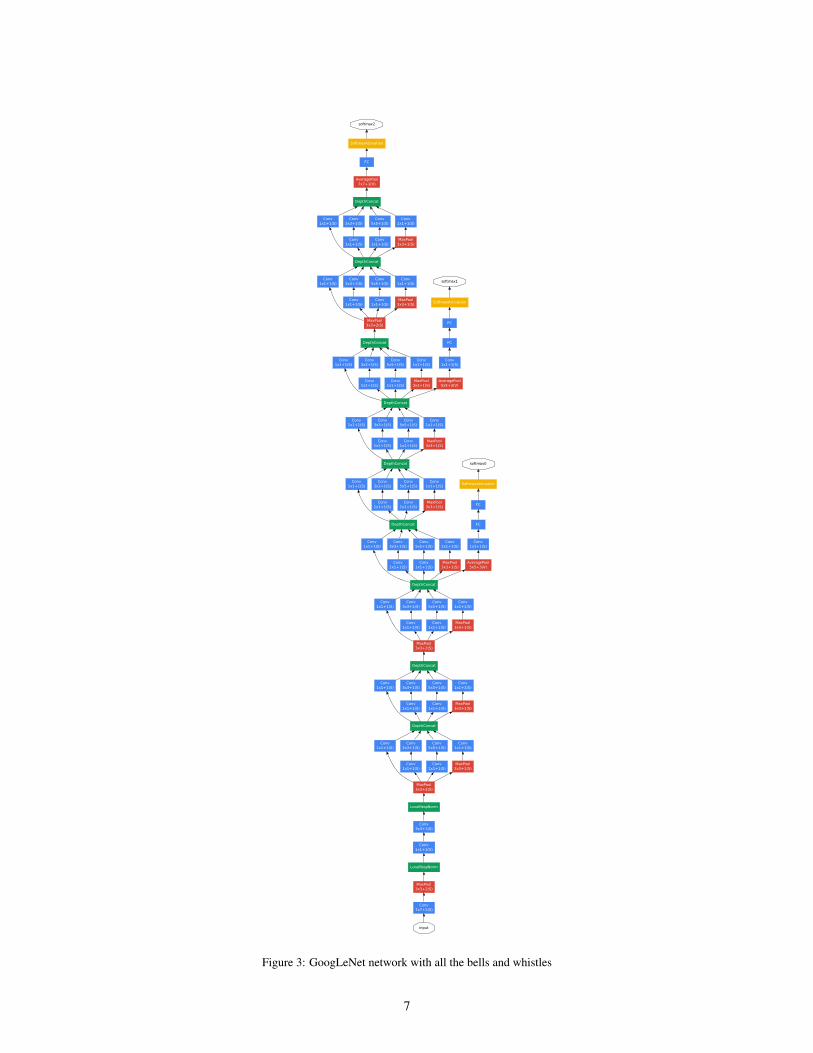
Figure 3: GoogLeNet network with all the bells and whistles

7

• A 1×1 convolution with 128 filters for dimension reduction and rectified linear activation.

• A fully connected layer with 1024 units and rectified linear activation.

• A dropout layer with 70% ratio of dropped outputs.

• A linear layer with softmax loss as the classifier (predicting the same 1000 classes as themain classifier, but removed at inference time).

A schematic view of the resulting network is depicted in Figure 3.

6 Training Methodology

Our networks were trained using the DistBelief [4] distributed machine learning system using mod-est amount of model and data-parallelism. Although we used CPU based implementation only, arough estimate suggests that the GoogLeNet network could be trained to convergence using fewhigh-end GPUs within a week, the main limitation being the memory usage. Our training usedasynchronous stochastic gradient descent with 0.9 momentum [17], fixed learning rate schedule (de-creasing the learning rate by 4% every 8 epochs). Polyak averaging [13] was used to create the finalmodel used at inference time.

Our image sampling methods have changed substantially over the months leading to the competition,and already converged models were trained on with other options, sometimes in conjunction withchanged hyperparameters, like dropout and learning rate, so it is hard to give a definitive guidanceto the most effective single way to train these networks. To complicate matters further, some ofthe models were mainly trained on smaller relative crops, others on larger ones, inspired by [8].Still, one prescription that was verified to work very well after the competition includes samplingof various sized patches of the image whose size is distributed evenly between 8% and 100% of theimage area and whose aspect ratio is chosen randomly between 3/4 and 4/3. Also, we found that thephotometric distortions by Andrew Howard [8] were useful to combat overfitting to some extent. Inaddition, we started to use random interpolation methods (bilinear, area, nearest neighbor and cubic,with equal probability) for resizing relatively late and in conjunction with other hyperparameterchanges, so we could not tell definitely whether the final results were affected positively by theiruse.

7 ILSVRC 2014 Classification Challenge Setup and Results

The ILSVRC 2014 classification challenge involves the task of classifying the image into one of1000 leaf-node categories in the Imagenet hierarchy. There are about 1.2 million images for training,50,000 for validation and 100,000 images for testing. Each image is associated with one groundtruth category, and performance is measured based on the highest scoring classifier predictions.Two numbers are usually reported: the top-1 accuracy rate, which compares the ground truth againstthe first predicted class, and the top-5 error rate, which compares the ground truth against the first5 predicted classes: an image is deemed correctly classified if the ground truth is among the top-5,regardless of its rank in them. The challenge uses the top-5 error rate for ranking purposes.

We participated in the challenge with no external data used for training. In addition to the trainingtechniques aforementioned in this paper, we adopted a set of techniques during testing to obtain ahigher performance, which we elaborate below.

1. We independently trained 7 versions of the same GoogLeNet model (including one widerversion), and performed ensemble prediction with them. These models were trained withthe same initialization (even with the same initial weights, mainly because of an oversight)and learning rate policies, and they only differ in sampling methodologies and the randomorder in which they see input images.

2. During testing, we adopted a more aggressive cropping approach than that of Krizhevsky etal. [9]. Specifically, we resize the image to 4 scales where the shorter dimension (height orwidth) is 256, 288, 320 and 352 respectively, take the left, center and right square of theseresized images (in the case of portrait images, we take the top, center and bottom squares).For each square, we then take the 4 corners and the center 224×224 crop as well as the

8

Team Year Place Error (top-5) Uses external data

SuperVision 2012 1st 16.4% no

SuperVision 2012 1st 15.3% Imagenet 22k

Clarifai 2013 1st 11.7% no

Clarifai 2013 1st 11.2% Imagenet 22k

MSRA 2014 3rd 7.35% no

VGG 2014 2nd 7.32% no

GoogLeNet 2014 1st 6.67% no

Table 2: Classification performance

Number of models Number of Crops Cost Top-5 error compared to base1 1 1 10.07% base

1 10 10 9.15% -0.92%

1 144 144 7.89% -2.18%

7 1 7 8.09% -1.98%

7 10 70 7.62% -2.45%

7 144 1008 6.67% -3.45%

Table 3: GoogLeNet classification performance break down

square resized to 224×224, and their mirrored versions. This results in 4×3×6×2 = 144crops per image. A similar approach was used by Andrew Howard [8] in the previous year’sentry, which we empirically verified to perform slightly worse than the proposed scheme.We note that such aggressive cropping may not be necessary in real applications, as thebenefit of more crops becomes marginal after a reasonable number of crops are present (aswe will show later on).

3. The softmax probabilities are averaged over multiple crops and over all the individual clas-sifiers to obtain the final prediction. In our experiments we analyzed alternative approacheson the validation data, such as max pooling over crops and averaging over classifiers, butthey lead to inferior performance than the simple averaging.

In the remainder of this paper, we analyze the multiple factors that contribute to the overall perfor-mance of the final submission.

Our final submission in the challenge obtains a top-5 error of 6.67% on both the validation andtesting data, ranking the first among other participants. This is a 56.5% relative reduction comparedto the SuperVision approach in 2012, and about 40% relative reduction compared to the previousyear’s best approach (Clarifai), both of which used external data for training the classifiers. Thefollowing table shows the statistics of some of the top-performing approaches.

We also analyze and report the performance of multiple testing choices, by varying the number ofmodels and the number of crops used when predicting an image in the following table. When weuse one model, we chose the one with the lowest top-1 error rate on the validation data. All numbersare reported on the validation dataset in order to not overfit to the testing data statistics.

8 ILSVRC 2014 Detection Challenge Setup and Results

The ILSVRC detection task is to produce bounding boxes around objects in images among 200possible classes. Detected objects count as correct if they match the class of the groundtruth andtheir bounding boxes overlap by at least 50% (using the Jaccard index). Extraneous detections countas false positives and are penalized. Contrary to the classification task, each image may contain

9

Team Year Place mAP external data ensemble approachUvA-Euvision 2013 1st 22.6% none ? Fisher vectors

Deep Insight 2014 3rd 40.5% ImageNet 1k 3 CNN

CUHK DeepID-Net 2014 2nd 40.7% ImageNet 1k ? CNN

GoogLeNet 2014 1st 43.9% ImageNet 1k 6 CNN

Table 4: Detection performance

Team mAP Contextual model Bounding box regressionTrimps-Soushen 31.6% no ?

Berkeley Vision 34.5% no yes

UvA-Euvision 35.4% ? ?

CUHK DeepID-Net2 37.7% no ?

GoogLeNet 38.02% no no

Deep Insight 40.2% yes yes

Table 5: Single model performance for detection

many objects or none, and their scale may vary from large to tiny. Results are reported using themean average precision (mAP).

The approach taken by GoogLeNet for detection is similar to the R-CNN by [6], but is augmentedwith the Inception model as the region classifier. Additionally, the region proposal step is improvedby combining the Selective Search [20] approach with multi-box [5] predictions for higher objectbounding box recall. In order to cut down the number of false positives, the superpixel size wasincreased by 2×. This halves the proposals coming from the selective search algorithm. We addedback 200 region proposals coming from multi-box [5] resulting, in total, in about 60% of the pro-posals used by [6], while increasing the coverage from 92% to 93%. The overall effect of cutting thenumber of proposals with increased coverage is a 1% improvement of the mean average precisionfor the single model case. Finally, we use an ensemble of 6 ConvNets when classifying each regionwhich improves results from 40% to 43.9% accuracy. Note that contrary to R-CNN, we did not usebounding box regression due to lack of time.

We first report the top detection results and show the progress since the first edition of the detectiontask. Compared to the 2013 result, the accuracy has almost doubled. The top performing teams alluse Convolutional Networks. We report the official scores in Table 4 and common strategies for eachteam: the use of external data, ensemble models or contextual models. The external data is typicallythe ILSVRC12 classification data for pre-training a model that is later refined on the detection data.Some teams also mention the use of the localization data. Since a good portion of the localizationtask bounding boxes are not included in the detection dataset, one can pre-train a general boundingbox regressor with this data the same way classification is used for pre-training. The GoogLeNetentry did not use the localization data for pretraining.

In Table 5, we compare results using a single model only. The top performing model is by DeepInsight and surprisingly only improves by 0.3 points with an ensemble of 3 models while theGoogLeNet obtains significantly stronger results with the ensemble.

9 Conclusions

Our results seem to yield a solid evidence that approximating the expected optimal sparse structureby readily available dense building blocks is a viable method for improving neural networks forcomputer vision. The main advantage of this method is a significant quality gain at a modest in-crease of computational requirements compared to shallower and less wide networks. Also note thatour detection work was competitive despite of neither utilizing context nor performing bounding box

10

regression and this fact provides further evidence of the strength of the Inception architecture. Al-though it is expected that similar quality of result can be achieved by much more expensive networksof similar depth and width, our approach yields solid evidence that moving to sparser architecturesis feasible and useful idea in general. This suggest promising future work towards creating sparserand more refined structures in automated ways on the basis of [2].

10 Acknowledgements

We would like to thank Sanjeev Arora and Aditya Bhaskara for fruitful discussions on [2]. Alsowe are indebted to the DistBelief [4] team for their support especially to Rajat Monga, Jon Shlens,Alex Krizhevsky, Jeff Dean, Ilya Sutskever and Andrea Frome. We would also like to thank to TomDuerig and Ning Ye for their help on photometric distortions. Also our work would not have beenpossible without the support of Chuck Rosenberg and Hartwig Adam.

References

[1] Know your meme: We need to go deeper. http://knowyourmeme.com/memes/we-need-to-go-deeper. Accessed: 2014-09-15.

[2] Sanjeev Arora, Aditya Bhaskara, Rong Ge, and Tengyu Ma. Provable bounds for learningsome deep representations. CoRR, abs/1310.6343, 2013.

[3] Umit V. Catalyurek, Cevdet Aykanat, and Bora Ucar. On two-dimensional sparse matrix par-titioning: Models, methods, and a recipe. SIAM J. Sci. Comput., 32(2):656–683, February2010.

[4] Jeffrey Dean, Greg Corrado, Rajat Monga, Kai Chen, Matthieu Devin, Mark Mao,Marc’aurelio Ranzato, Andrew Senior, Paul Tucker, Ke Yang, Quoc V. Le, and Andrew Y.Ng. Large scale distributed deep networks. In P. Bartlett, F.c.n. Pereira, C.j.c. Burges, L. Bot-tou, and K.q. Weinberger, editors, Advances in Neural Information Processing Systems 25,pages 1232–1240. 2012.

[5] Dumitru Erhan, Christian Szegedy, Alexander Toshev, and Dragomir Anguelov. Scalable ob-ject detection using deep neural networks. In Computer Vision and Pattern Recognition, 2014.CVPR 2014. IEEE Conference on, 2014.

[6] Ross B. Girshick, Jeff Donahue, Trevor Darrell, and Jitendra Malik. Rich feature hierarchiesfor accurate object detection and semantic segmentation. In Computer Vision and PatternRecognition, 2014. CVPR 2014. IEEE Conference on, 2014.

[7] Geoffrey E. Hinton, Nitish Srivastava, Alex Krizhevsky, Ilya Sutskever, and Ruslan Salakhut-dinov. Improving neural networks by preventing co-adaptation of feature detectors. CoRR,abs/1207.0580, 2012.

[8] Andrew G. Howard. Some improvements on deep convolutional neural network based imageclassification. CoRR, abs/1312.5402, 2013.

[9] Alex Krizhevsky, Ilya Sutskever, and Geoff Hinton. Imagenet classification with deep con-volutional neural networks. In Advances in Neural Information Processing Systems 25, pages1106–1114, 2012.

[10] Y. LeCun, B. Boser, J. S. Denker, D. Henderson, R. E. Howard, W. Hubbard, and L. D. Jackel.Backpropagation applied to handwritten zip code recognition. Neural Comput., 1(4):541–551,December 1989.

[11] Yann LeCun, Leon Bottou, Yoshua Bengio, and Patrick Haffner. Gradient-based learningapplied to document recognition. Proceedings of the IEEE, 86(11):2278–2324, 1998.

[12] Min Lin, Qiang Chen, and Shuicheng Yan. Network in network. CoRR, abs/1312.4400, 2013.

[13] B. T. Polyak and A. B. Juditsky. Acceleration of stochastic approximation by averaging. SIAMJ. Control Optim., 30(4):838–855, July 1992.

[14] Pierre Sermanet, David Eigen, Xiang Zhang, Michael Mathieu, Rob Fergus, and Yann Le-Cun. Overfeat: Integrated recognition, localization and detection using convolutional net-works. CoRR, abs/1312.6229, 2013.

11

[15] Thomas Serre, Lior Wolf, Stanley M. Bileschi, Maximilian Riesenhuber, and Tomaso Poggio.Robust object recognition with cortex-like mechanisms. IEEE Trans. Pattern Anal. Mach.Intell., 29(3):411–426, 2007.

[16] Fengguang Song and Jack Dongarra. Scaling up matrix computations on shared-memorymanycore systems with 1000 cpu cores. In Proceedings of the 28th ACM International Con-ference on Supercomputing, ICS ’14, pages 333–342, New York, NY, USA, 2014. ACM.

[17] Ilya Sutskever, James Martens, George E. Dahl, and Geoffrey E. Hinton. On the importanceof initialization and momentum in deep learning. In Proceedings of the 30th InternationalConference on Machine Learning, ICML 2013, Atlanta, GA, USA, 16-21 June 2013, volume 28of JMLR Proceedings, pages 1139–1147. JMLR.org, 2013.

[18] Christian Szegedy, Alexander Toshev, and Dumitru Erhan. Deep neural networks for objectdetection. In Christopher J. C. Burges, Leon Bottou, Zoubin Ghahramani, and Kilian Q.Weinberger, editors, Advances in Neural Information Processing Systems 26: 27th AnnualConference on Neural Information Processing Systems 2013. Proceedings of a meeting heldDecember 5-8, 2013, Lake Tahoe, Nevada, United States., pages 2553–2561, 2013.

[19] Alexander Toshev and Christian Szegedy. Deeppose: Human pose estimation via deep neuralnetworks. CoRR, abs/1312.4659, 2013.

[20] Koen E. A. van de Sande, Jasper R. R. Uijlings, Theo Gevers, and Arnold W. M. Smeulders.Segmentation as selective search for object recognition. In Proceedings of the 2011 Interna-tional Conference on Computer Vision, ICCV ’11, pages 1879–1886, Washington, DC, USA,2011. IEEE Computer Society.

[21] Matthew D. Zeiler and Rob Fergus. Visualizing and understanding convolutional networks. InDavid J. Fleet, Tomas Pajdla, Bernt Schiele, and Tinne Tuytelaars, editors, Computer Vision- ECCV 2014 - 13th European Conference, Zurich, Switzerland, September 6-12, 2014, Pro-ceedings, Part I, volume 8689 of Lecture Notes in Computer Science, pages 818–833. Springer,2014.

12