Institut d’Economie Industrielle (IDEI) – Manufacture des TabacsAile Jean-Jacques Laffont – 21, allée de Brienne – 31000 TOULOUSE – FRANCETél. + 33(0)5 61 12 85 89 – Fax + 33(0)5 61 12 86 37 – www.idei.fr – contact@cict.fr

September, 2010

n° 649

“Going for Broke: New Century Financial Corporation,

2004-2006”

Augustin LANDIER, David SRAER, and David THESMAR

Going for broke: New Century Financial Corporation, 2004-20061

Augustin Landier (Toulouse School of Economics) David Sraer (Princeton University) David Thesmar (HEC & CEPR) September 2010 PRELIMINARY VERSION Abstract: Using loan level data, we investigate the lending behavior of a large subprime mortgage issuer prior to its bankruptcy in the beginning of 2007. In 2004, this firm suddenly started to massively issue new loans contracts that featured deferred amortization ("interest-only loans") to high income and high FICO households. We document that these loans were not only riskier, but also that their returns were more sensitive to real estate prices than standard contracts. Implicitly, this lender dramatically increased its exposure to its own legacy asset, which is what a standard model of portfolio selection in distress would predict. We provide additional evidence on New Century’s lending behavior, which are consistent with a risk shifting strategy. Finally, we are able to tie this sudden change in behavior to the sharp monetary policy tightening implemented by the Fed in the spring of 2004. Our findings shed new light on the relationship between monetary policy and risk taking by financial institutions.

1 We thank for their inputs at a preliminary stage of this project Harrison Hong, Florencio Lopez-de-Silanes, José Scheinkman and Andrei Shleifer. We thank Adrien Matray for valuable research assistance.

1. Introduction The costs of financial distress (CFD) incurred by firms at high leverage levels are at the core of modern corporate finance theory. In the “trade-off” view of capital structure, firms pick their capital structure ex-ante such as to maximize gains from debt (tax shield, incentive effect), net of the present value of the costs of financial distress2

. However, little is known about the exact quantification of these costs and the timing of their occurrence. The reason is that the direct costs of financial distress (such as lawyer bills, managerial distraction, or customers churn) are only a small fraction of the total costs of financial distress (see e.g. Andrade and Kaplan 1998); instead, the bulk of these costs are indirect: they come from distortions in project selection induced by high leverage. A major class of such distortions is risk shifting: an institution in distress is biased toward projects that pay-off in the state of the world where it escapes bankruptcy (the seminal model of risk-shifting is Stiglitz and Weiss, 1983). Such biased project choice can lead to the selection of negative NPV projects, while remaining compatible with ex-post shareholder value maximization.

This paper provides new evidence on the impact of high financial leverage on project choice by examining the second-largest subprime mortgage lender in the United States, New Century Financial Corporation from 2001 till its bankruptcy filing in February 2007. As described in detail in the next section, New Century was focused on the subprime segment of the mortgage market, lending primarily to individuals who “do not satisfy the credit, documentation or other underwriting standards prescribed by conventional mortgage lenders and loan buyers”.3

While NC was selling some of its loans to third parties after originating them, it was also retaining an important fraction of it for investment as an asset on its balance sheet (up to $11bn in 2005, i.e. more than 20% of originated loans). As a consequence, the sharp increase in interest rates that was initiated by the Fed in 2004 constituted a highly negative shock to the value of NC’s existing assets relative to its liabilities. Beyond this effect on NC’s legacy asset, the 2004 monetary shock materialized in lower growth opportunities in its existing market.

Using data on loans issued by New Century, we find that New Century sharply modified its origination process starting in 2004. It started issuing loans with payoffs contingent on the bubble continuing over the next 2-3 years. In short, NC implemented a “go-for-broke” strategy, paying off only in case of continuingly strong real estate prices. This strategic shift involved both a change in the nature of financial contracts and in the customer base targeted by NC. More precisely, NC moved away from traditional "hybrid" adjustable rate mortgages and started massively issuing loans featuring deferred amortization ("interest-only loans"). These loans were issued primarily toward high income and high FICO households. Using data on loans serviced by NC, we find that the payoffs of “interest-only” loans were riskier and, importantly, more sensitive to real estate prices than standard contracts. One contractual characteristic of these loans is to exhibit a strong jump in due repayments at a reset date (typically 24 months from origination). Because of this contractual feature (referred to internally in NC as a “sticker shock”4

2 For an attempt at quantifying these CFD using corporate bond spreads, see Almeida and Philippon (2007).

), these loans would

3 10K filings, 2005, available on the SEC web site. 4 See Missal (2008).

eventually pay off only if the borrower could refinance at that reset date, which would require sustained real estate prices growth. If prices had ceased to grow within the 24 months following issuance, such loans would be much less likely to be repaid, either because the borrower would strategically default, or because competitors would be unwilling to refinance the loan. Thus, the exposure of NC to real estate prices movements was substantially increased by this strategic shift. This is consistent with the view that NC was “gambling for resurrection”, by financing projects paying off only in the “good state”. We provide further evidence of such risk shifting behavior by NC. In particular, a standard model of portfolio selection in distress predicts that once in distress, a firm should increase its exposure to its own legacy asset. In line with this idea, we find that NC tilted its customer basis toward regions with a high beta on its existing asset pool of loans. The evidence that “interest-only” loans were primarily sold to high FICO, high income borrowers can also be interpreted at the light of this risk shifting behavior, as skilled workers tend to have more pro-cyclical labor income (see Parker and Vissing-Jorgensen, 2009). We view the contributions of our paper are threefold. First, the paper sheds light on the behavior of a financial institution in financial distress. This is related e.g. to Esty (1997) who finds compelling evidence of shareholder value maximizing risk shifting during the savings and loans crisis. He does so by comparing the strategies followed by similar financial institutions differing only in organizational forms. Our paper shows that risk shifting is characterized not only by the choice to hold more volatile assets but more specifically by the choice of new assets that have a high beta on existing assets. Consistent with this idea, NC reaction to the sharp increase in interest rates in 2004 was to issuing highly “price-contingent” loans, paying off only in case of sustained real estate price growth. As a consequence, loans issued by NC after 2004 became much more likely to default should the bubble burst. During bubbles, this mechanism can have a strong reinforcing effect: it creates a reason for the more fragile institutions to “ride the bubble”, potentially aggravating the consequences of a burst. Second, we provide a new perspective on the narrative of the 2007 financial crisis, in particular concerning the role of mortgage originators, who were key players in the subprime meltdown. Many existing comments on the role of originators insist on their lack of incentives to monitor loan quality, as these loans were passed on to final investors (for instance, Mian and Sufi, 2009, Keys et al., 2010). New Century’s behavior, and possibly that of other originators, does not fit this model: 5 we describe how New Century kept a large fraction of the loans it originated on its balance sheet6

5 In the same vein, Acharya et al. (2010) show that securitization was not always riskless for the banks that securitized. In some vehicles, the issuing bank provided investors an explicit guarantee over their investment, in case underlying loans would default. In these particular circumstances, the bank was still bearing the risk of the loans it did securitize, so the "lack of incentive to screen" story fails to apply, as in the NC case.

. More precisely, we argue that, in mid 2004, precisely because of these assets and their expected loss of value, NC started to gamble for resurrection by issuing riskier loans. Mayer et al., 2010, document the spread of negative amortization mortgages. We document the massive introduction of these products

6 NC was not an exception with that regard. Its main pure-play competitor, Countrywide held $39 Bil. worth of mortgages for investment on its balance sheet in 2004, which was about 1/3 of its total assets.

by NC in 2004 and offer an explanation for their use that is consistent with shareholder value maximization. We are thus in line with a view of the crisis where risk was undertaken ex-post at the expense of debt holders but at the advantage of shareholders. This is close to the view developed in Hong and Scheinkman (2010), who show that the banks taking high risks pre-crisis were doing so to cater to the preferences of shareholders. Our risk-shifting narrative is highly different from a “looting view" of the crisis, whereby banks' executives, salesmen and traders would destroy the value of the firm due to highly convex or short-term incentives, leading to high ex-post inefficiencies (Akerlof and Romer, 1993, LaPorta et al., 2003, Kashyap et al., 2009, Biais et al., 2010). It also differs from a “catering view” whereby the crisis results from financial institutions producing toxic financial assets catering to the demand of “naïve” or “subsidized” investors (Shleifer and Vishny, 2010, Nadauld and Weisbach, 2010). The difficulties with that view is to explain why originators of those assets kept so much exposure to them, which in our case is a simple consequence of the mechanism at play (risk shifting), not a puzzle. Last, our paper puts in perspective an under-investigated aspect of monetary policy: It is often argued that low interest rates were the source of excess risk-shifting by making investors desperate for yield. For instance, Yellen 2010 states that “It is conceivable that accommodative monetary policy could provide tinder for a buildup of leverage and excessive risk-taking in the financial system”7

. The view the Fed’s persistent policy of low interest rates fuelled leveraging by financial institutions is also expressed by e.g. Rajan, 2005, Diamond and Rajan, 2009, or Stiglitz 2010. However, without contradicting that view, we point out that its implications for optimizing monetary policy are not simple: Increasing interest rates during a bubble might not have the sought after effect of decreasing risk-taking. Quite to the contrary, raising rates can exacerbate risk shifting, because it weakens the balance sheet of financial institutions. This is what happened to NC in 2004. This suggests that tightening of monetary policy after an exuberance phase, if too rapid, can lead to the creation of “zombie” financial institutions, which following the monetary shock are pushed into risk-shifting and might propagate rather than mitigate risk.

We proceed in four steps. Section 2 describes the data and the business of NC, with a special attention to the different types of contracts used by NC and to the trends observed in the composition of the loans it issued. Section 3 provides a simple framework to explain what projects a highly levered institution should select, when maximizing shareholder value. We show that together with volatility, the correlation structure between these new projects and the legacy projects appears to be a critical variable. Section 4 shows that the 2004 rise in interest rates was an important negative shock to NC’s existing assets and to its continuation value. Section 5 investigates risk-shifting behavior by NC and tests the finer predictions of this view: NC issues loans that are more price-dependent, with a higher beta on the existing asset. Section 6 concludes.

7 Yellen Janet, Oct. 2010, prepared remarks to the annual meeting of the National Association for Business Economics.

2. Data and business description

a. New Century’s business Looking at New Century’s business over the 2001-2005 period, the striking fact is that the company progressively moves away from a pure originate and distribute business model, where loans are only held temporarily on the balance sheet. As time passes, the company finds itself holding more and more loans for the long term, and its balance sheet explodes. But let us first review the three main ways for New Century to finance loan issuance.

[Insert Table 1 about here]

Whole loan sales New century issues (« originates ») mortgage loans. Most of them are sold within a few months to third parties (mostly investment banks that will eventually repackage them) through what is called « whole loan sales ». Since the ownership transfer takes a few months, New Century always holds an inventory that is typically financed by short term financing (credit lines). The ratio of inventories to total originations increases modestly over time, suggesting that NC progressively finds it harder to sell the loans it issues. It goes from about 52 days in 2002 to 68 days in 2005. The increase remains, however, moderate, given the very rapid pace of expansion in NC’s activities: whole loans sales are multiplied by 7,5 between 2001 and 2005. This part of NC’s activities generates off-balance sheet liabilities, but it is not obvious to quantify their extent. First, buyers can return loans that default within a few months of origination (early payment defaults). Second, NC is forced to replace or repurchase loans if buyers can prove a breach of representation or warranty by the lender.8

Securitization structured as sale This is the standard securitization. In this setting, NC would set up a trust, which would receive loans as assets. The trust would issue bonds that will receive principal repayment plus an interest that is lower than the interest rate actually paid by the loans. This is in exchange for seniority. NC would receive the residual and book it as income. Securitization structured as sale is a small and intermittent share of total originations. There is none in 2003 and 2004. In 2002, it is about 10% of total originations. In 2001 and 2005, it hovers around 10-12%.

8 « We sell whole loans on a non-recourse basis pursuant to a purchase agreement in which we give customary representations and warranties regarding the loan characteristics and the origination process. Therefore, we may be required to repurchase or substitute loans in the event of a breach of these representations and warranties. In addition, we generally commit to repurchase or substitute a loan if a payment default occurs within the first month or two following the date the loan is funded, unless we make other arrangements with the purchaser. » (10k form for fiscal year 2003, p13)

As for whole loan sales, off-balance sheet liabilities seem to be limited to breach of representation or warranty. 9

Securitization structured as financing This is the last category, and here loans that are issued fully remain on NC’s balance sheet. This category of financing has dramatically increased over the period, from zero in 2001 and 2002 to $11bn in 2005 (about 20% of overall originations). In this case, New Century becomes in effect a mortgage lender. Financing of these assets is done through the issue of bonds, who rise in NC’s balance sheet in parallel with the corresponding assets; these bonds are collateralized by the loans, but nowhere in the 10K filings could we find a sentence mentioning that these bondholders had no recourse to NC. It seems a priori reasonable to assume that these bonds were sold with recourse, so that NC's shareholders are liable for defaults on these loans.

[Insert Table 2 about here]

Looking at overall capital structure, the dramatic increase in the importance of these loans and their financing leads to a sharp increase in the gearing ratio (book value of debt to book value of equity): 5 (2002), to 11 (2005). This is apparent from Table 2, which reports the evolution of a stylized balance sheet from 2001 to 2005 (last year for which we have annual accounts).

b. Data We use several sources of data. New Century’s loan database

[Insert Figure 1 about here]

The loan database we use is a 20% random extract of the exhaustive loan database used by New Century when it was in operation. It contains 739,688 loan applications examined by NC since 1997. These data are used in the academic literature by Berndt and al., 2010, who analyze incentives of mortgage brokers. Figure 1 shows how steep NC’s growth has been since 2002-2003. Until 2001, the firm was examining about 20,000 applications a year. The annual flow increases to about 100,000 in 2003 to culminate around 160,000 in 2004-2005. This corresponds to an eightfold increase in NC’s volume of activity in about 3 years (from 2002 to 2004). Such an amazing growth is consistent with aggregate origination figures from Table 1: the loan-level data are consistent with accounting information from the 10k filings.

9 « The Certificates are typically sold at face value and without recourse except that the Company provides representations and warranties customary to the mortgage banking industry to the Trust. » Source: 2003 10K filing. In 2005, the 10K filing makes a somewhat more mysterious statement: «We are party to various transactions that have an off-balance sheet component. In connection with our off-balance sheet securitization transactions, there were $6.9 billion in loans owned by the off-balance sheet trusts as of December 31, 2005. The trusts have issued bonds secured by these loans. The bondholders generally do not have recourse to us in the event that the loans in the various trusts do not perform as expected except for specific circumstances. »

The loan database reports a large number of variables. We will just use a few:

- Borrower: full documentation provided (or not), loan to value ratio, income, fico score, age

- Property: zip code - Loan: principal, status (funded, denied by NC, withdrawn by borrower), fixed or

variable rate (ARM or FRM), maturity (30 years for 92% of the applications), interest rate, amortization schedule (is there an interest only period or a balloon dimension), length of the teaser period (2 to 5 years), purpose of the loan (first purchase or refinancing), first monthly payment, etc.

[Insert Tables 3 and 4 about here]

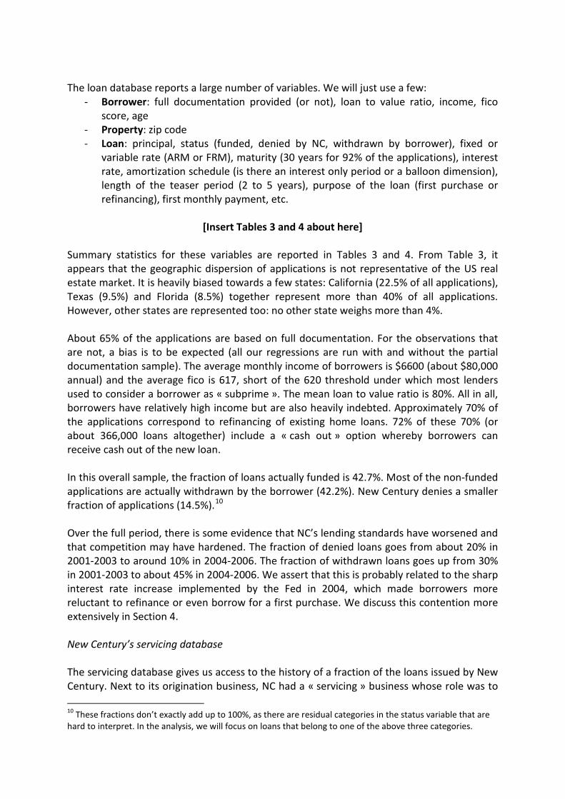
Summary statistics for these variables are reported in Tables 3 and 4. From Table 3, it appears that the geographic dispersion of applications is not representative of the US real estate market. It is heavily biased towards a few states: California (22.5% of all applications), Texas (9.5%) and Florida (8.5%) together represent more than 40% of all applications. However, other states are represented too: no other state weighs more than 4%. About 65% of the applications are based on full documentation. For the observations that are not, a bias is to be expected (all our regressions are run with and without the partial documentation sample). The average monthly income of borrowers is $6600 (about $80,000 annual) and the average fico is 617, short of the 620 threshold under which most lenders used to consider a borrower as « subprime ». The mean loan to value ratio is 80%. All in all, borrowers have relatively high income but are also heavily indebted. Approximately 70% of the applications correspond to refinancing of existing home loans. 72% of these 70% (or about 366,000 loans altogether) include a « cash out » option whereby borrowers can receive cash out of the new loan. In this overall sample, the fraction of loans actually funded is 42.7%. Most of the non-funded applications are actually withdrawn by the borrower (42.2%). New Century denies a smaller fraction of applications (14.5%).10

Over the full period, there is some evidence that NC’s lending standards have worsened and that competition may have hardened. The fraction of denied loans goes from about 20% in 2001-2003 to around 10% in 2004-2006. The fraction of withdrawn loans goes up from 30% in 2001-2003 to about 45% in 2004-2006. We assert that this is probably related to the sharp interest rate increase implemented by the Fed in 2004, which made borrowers more reluctant to refinance or even borrow for a first purchase. We discuss this contention more extensively in Section 4. New Century’s servicing database The servicing database gives us access to the history of a fraction of the loans issued by New Century. Next to its origination business, NC had a « servicing » business whose role was to 10 These fractions don’t exactly add up to 100%, as there are residual categories in the status variable that are hard to interpret. In the analysis, we will focus on loans that belong to one of the above three categories.

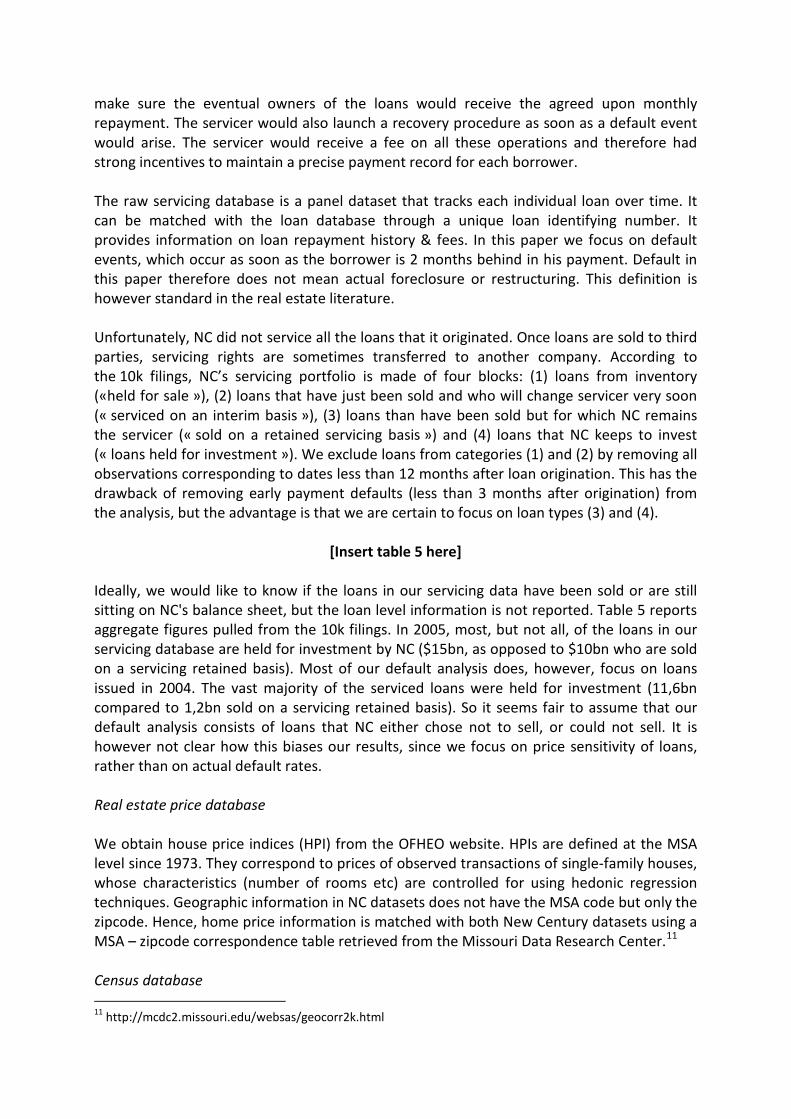
make sure the eventual owners of the loans would receive the agreed upon monthly repayment. The servicer would also launch a recovery procedure as soon as a default event would arise. The servicer would receive a fee on all these operations and therefore had strong incentives to maintain a precise payment record for each borrower. The raw servicing database is a panel dataset that tracks each individual loan over time. It can be matched with the loan database through a unique loan identifying number. It provides information on loan repayment history & fees. In this paper we focus on default events, which occur as soon as the borrower is 2 months behind in his payment. Default in this paper therefore does not mean actual foreclosure or restructuring. This definition is however standard in the real estate literature. Unfortunately, NC did not service all the loans that it originated. Once loans are sold to third parties, servicing rights are sometimes transferred to another company. According to the 10k filings, NC’s servicing portfolio is made of four blocks: (1) loans from inventory («held for sale »), (2) loans that have just been sold and who will change servicer very soon (« serviced on an interim basis »), (3) loans than have been sold but for which NC remains the servicer (« sold on a retained servicing basis ») and (4) loans that NC keeps to invest (« loans held for investment »). We exclude loans from categories (1) and (2) by removing all observations corresponding to dates less than 12 months after loan origination. This has the drawback of removing early payment defaults (less than 3 months after origination) from the analysis, but the advantage is that we are certain to focus on loan types (3) and (4).

[Insert table 5 here]

Ideally, we would like to know if the loans in our servicing data have been sold or are still sitting on NC's balance sheet, but the loan level information is not reported. Table 5 reports aggregate figures pulled from the 10k filings. In 2005, most, but not all, of the loans in our servicing database are held for investment by NC ($15bn, as opposed to $10bn who are sold on a servicing retained basis). Most of our default analysis does, however, focus on loans issued in 2004. The vast majority of the serviced loans were held for investment (11,6bn compared to 1,2bn sold on a servicing retained basis). So it seems fair to assume that our default analysis consists of loans that NC either chose not to sell, or could not sell. It is however not clear how this biases our results, since we focus on price sensitivity of loans, rather than on actual default rates. Real estate price database We obtain house price indices (HPI) from the OFHEO website. HPIs are defined at the MSA level since 1973. They correspond to prices of observed transactions of single-family houses, whose characteristics (number of rooms etc) are controlled for using hedonic regression techniques. Geographic information in NC datasets does not have the MSA code but only the zipcode. Hence, home price information is matched with both New Century datasets using a MSA – zipcode correspondence table retrieved from the Missouri Data Research Center.11

Census database 11 http://mcdc2.missouri.edu/websas/geocorr2k.html

Some borrower specific information such as education, are not available from NC’s loan database. To fill this gap, we retrieve average education in 2000 by census tract using a 5% extract of the 2000 census (itself obtained from the PUMS website12

). We then match this information with NC datasets using a correspondence table between zip codes and census tract identifiers retrieved from the Missouri Data Center. A complication arises from the fact that some zip codes overlap several census tracts and some census tracts overlap several zip codes. Fortunately, the MDC provides us with the population in each tract x zip region, so that we end up taking, for each zip code, the average education level across tracts in this zip code, weighted by the population of each tract in this zip code.

c. The loan portfolio: trends This section documents a sharp change in the customer base and product mix of New Century in 2004. Starting in 2004, the firm started to originate loans with a strong deferred amortization feature; it also started to target richer but also more indebted borrowers with higher FICO scores. Safer, younger, richer borrowers

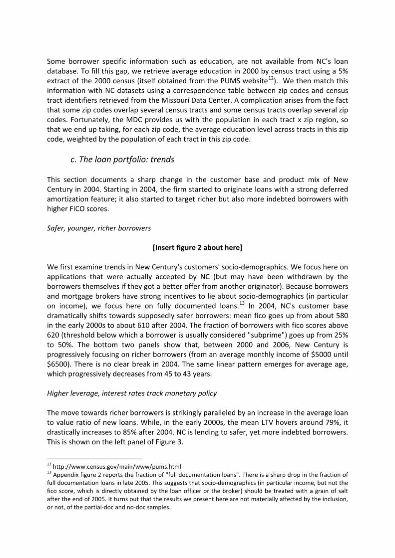
[Insert figure 2 about here]

We first examine trends in New Century's customers' socio-demographics. We focus here on applications that were actually accepted by NC (but may have been withdrawn by the borrowers themselves if they got a better offer from another originator). Because borrowers and mortgage brokers have strong incentives to lie about socio-demographics (in particular on income), we focus here on fully documented loans.13

In 2004, NC's customer base dramatically shifts towards supposedly safer borrowers: mean fico goes up from about 580 in the early 2000s to about 610 after 2004. The fraction of borrowers with fico scores above 620 (threshold below which a borrower is usually considered "subprime") goes up from 25% to 50%. The bottom two panels show that, between 2000 and 2006, New Century is progressively focusing on richer borrowers (from an average monthly income of $5000 until $6500). There is no clear break in 2004. The same linear pattern emerges for average age, which progressively decreases from 45 to 43 years.

Higher leverage, interest rates track monetary policy The move towards richer borrowers is strikingly paralleled by an increase in the average loan to value ratio of new loans. While, in the early 2000s, the mean LTV hovers around 79%, it drastically increases to 85% after 2004. NC is lending to safer, yet more indebted borrowers. This is shown on the left panel of Figure 3.

12 http://www.census.gov/main/www/pums.html 13 Appendix figure 2 reports the fraction of "full documentation loans". There is a sharp drop in the fraction of full documentation loans in late 2005. This suggests that socio-demographics (in particular income, but not the fico score, which is directly obtained by the loan officer or the broker) should be treated with a grain of salt after the end of 2005. It turns out that the results we present here are not materially affected by the inclusion, or not, of the partial-doc and no-doc samples.

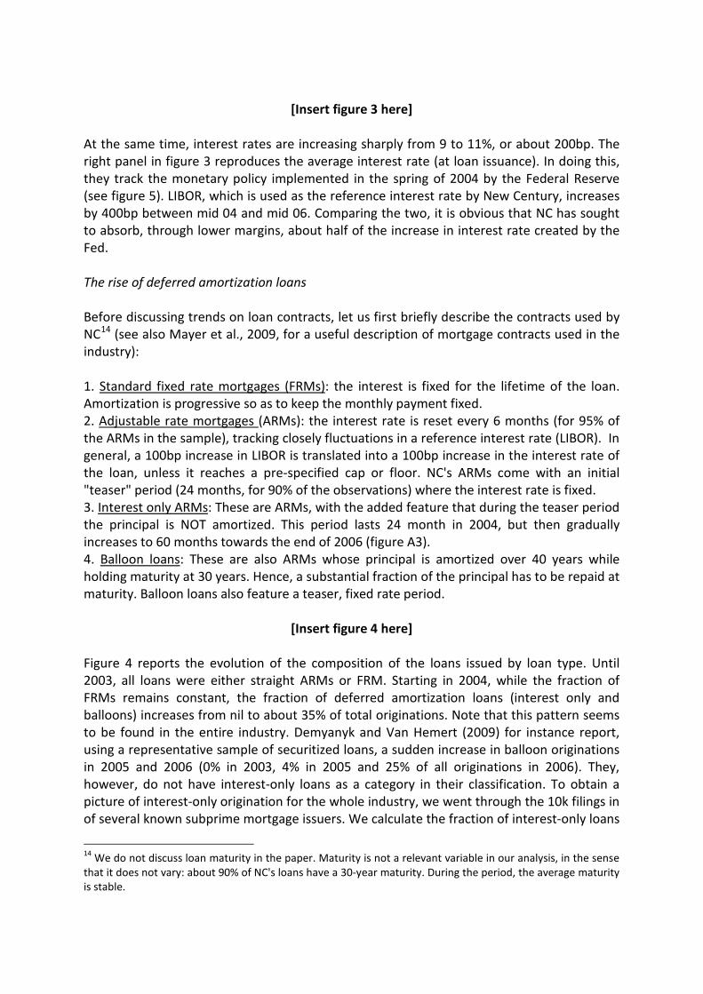
[Insert figure 3 here]

At the same time, interest rates are increasing sharply from 9 to 11%, or about 200bp. The right panel in figure 3 reproduces the average interest rate (at loan issuance). In doing this, they track the monetary policy implemented in the spring of 2004 by the Federal Reserve (see figure 5). LIBOR, which is used as the reference interest rate by New Century, increases by 400bp between mid 04 and mid 06. Comparing the two, it is obvious that NC has sought to absorb, through lower margins, about half of the increase in interest rate created by the Fed. The rise of deferred amortization loans Before discussing trends on loan contracts, let us first briefly describe the contracts used by NC14

(see also Mayer et al., 2009, for a useful description of mortgage contracts used in the industry):

1. Standard fixed rate mortgages (FRMs): the interest is fixed for the lifetime of the loan. Amortization is progressive so as to keep the monthly payment fixed. 2. Adjustable rate mortgages (ARMs): the interest rate is reset every 6 months (for 95% of the ARMs in the sample), tracking closely fluctuations in a reference interest rate (LIBOR). In general, a 100bp increase in LIBOR is translated into a 100bp increase in the interest rate of the loan, unless it reaches a pre-specified cap or floor. NC's ARMs come with an initial "teaser" period (24 months, for 90% of the observations) where the interest rate is fixed. 3. Interest only ARMs: These are ARMs, with the added feature that during the teaser period the principal is NOT amortized. This period lasts 24 month in 2004, but then gradually increases to 60 months towards the end of 2006 (figure A3). 4. Balloon loans: These are also ARMs whose principal is amortized over 40 years while holding maturity at 30 years. Hence, a substantial fraction of the principal has to be repaid at maturity. Balloon loans also feature a teaser, fixed rate period.

[Insert figure 4 here]

Figure 4 reports the evolution of the composition of the loans issued by loan type. Until 2003, all loans were either straight ARMs or FRM. Starting in 2004, while the fraction of FRMs remains constant, the fraction of deferred amortization loans (interest only and balloons) increases from nil to about 35% of total originations. Note that this pattern seems to be found in the entire industry. Demyanyk and Van Hemert (2009) for instance report, using a representative sample of securitized loans, a sudden increase in balloon originations in 2005 and 2006 (0% in 2003, 4% in 2005 and 25% of all originations in 2006). They, however, do not have interest-only loans as a category in their classification. To obtain a picture of interest-only origination for the whole industry, we went through the 10k filings in of several known subprime mortgage issuers. We calculate the fraction of interest-only loans

14 We do not discuss loan maturity in the paper. Maturity is not a relevant variable in our analysis, in the sense that it does not vary: about 90% of NC's loans have a 30-year maturity. During the period, the average maturity is stable.

in total originations over the 2002-2006 period: quite clearly, NC's move toward deferred amortization is representative of the rest of the industry, confirming that there is no specific pathology in the firm we are studying (see appendix figure 3).

[Insert table 6 here]

Table 6 reports observable differences between loan contracts, for full doc loans only, and only for loans accepted (funded or withdrawn) after 2003. Deferred amortization contracts are designed for more levered loans (higher loan to value ratio) and higher income borrowers. The loan amount is higher by more than $50,000. There are, in addition, sizeable differences between interest only and balloon loans. Interest only loans are largely intended for first purchase loans, high income, high fico and young borrowers. In spite of strong leverage, their average interest payment is low: 6.8%. Balloon loans are aimed at riskier borrowers, with a lower fico score (587) and a lower income ($6349 monthly, compared to $7724 for interest only loans). Borrowers targeted by balloon loans also pay higher interest rates (8.2%). d. Summary We have here documented a very striking change in NC's product mix and consumer base. Hereafter, we will interpret it as evidence of risk shifting by a distressed institution, and provide further evidence consistent with this. But before doing this, let us look at the exact predictions of a canonical model of financial distress. Understanding these predictions will guide our empirical strategy. 3. Portfolio choice in financial distress: a simple framework We formalize project choice by a distressed institution in a simple one period model. The goal is twofold: (1) to convince the reader that as the probability of default increases, a company tilts its preferences in favor of projects with high beta on its existing asset and (2) to show that the probability of default of a company does not have to be large for such distortions in project choice to be important. In other words, faced with a higher default probability, a shareholder value maximizing company will pick projects that have both a high variance (the usual risk-shifting intuition) and a high correlation with existing assets. Specifically, we derive its investment criterion and explain how it becomes different from the NPV criterion. A company owns a legacy asset worth S0 at time zero. The payoff of the legacy asset at time one is (1 + 𝑅)𝑆0 where R is the random one period gross return for holding such asset. R has cumulative distribution F. The company has debt with face value D at time one. Thus, its default probability is:

1 − 𝑝 = 𝑃(𝑆0(1 + 𝑅) < 𝐷) = 𝐹 � 𝐷𝑆0− 1�

We assume a risk-neutral pricing kernel, which implies E(R)=rf, where rf is the risk-free rate. Now consider a marginal dollar that the company can invest on a marginal project that consumes one unit of capital at time zero and yields a return (1+u) at time 1. For instance, this marginal dollar could be held in cash (yielding the risk-free rate). How should the managers of the company evaluate such marginal project, from the point of view of their shareholders? Assume distributions are Gaussian. We can thus consider the linear projection of the project’s return u on the legacy asset’s return R :

𝑢 = 𝛼 + 𝛽𝑅 + 𝜀, where 𝐸(𝜀 |𝑅) = 0 and β is the beta of the project on the legacy asset:

𝛽 = �𝑣𝑎𝑟(𝑢)𝑣𝑎𝑟(𝑟)

�1/2

𝑐𝑜𝑟𝑟(𝑅,𝑢).

An increase in a project’s beta can come from either higher variance or higher correlation with the existing asset. The value of the project for the shareholders comes from the payoffs of the project received when the company is not bankrupt. The discounted value of the project’s payoff for the shareholders is thus15

𝑝

1 + 𝑟𝑓[1 + 𝛼 + 𝛽𝐸(𝑅 |1 + R >

D𝑆0

)]

:

Since the project is marginal, the survival probability, p, can be taken as exogenous in its valuation16

. A sufficient statistics to compare two projects is thus (𝛼,𝛽). Specifically, a project (𝛼1,𝛽1) is preferred to (𝛼2,𝛽2) if:

𝛼1 − 𝛼2 + 𝐸 �𝑅 �1 + R > D𝑆0� (𝛽1 − 𝛽2) > 0.

Whereas an NPV approach in comparing the projects would give a ranking independent of

the βs:

𝛼1 − 𝛼2 > 0.

The risk-free asset is a particular case of marginal investment where (𝛼 ,𝛽 ) = (𝑟𝑓, 0). Without further financial constraints, a project is better for shareholders than the risk-free investment if:

𝛼 − 𝑟𝑓 + 𝐸 �𝑅 �1 + R > D𝑆0� 𝛽 > 0.

15We use the orthogonality of the error term to R: ∫𝐸(𝜀 |R = x)1𝑥>𝐷

𝑆0−1𝑑𝐹=0.

16 A marginal project only has, through its first-order impact on default, a second order impact on the shareholder value of the legacy asset. This is because at the default frontier, shareholder payoffs from the legacy asset equal zero, thus a first order change in the default frontier only impacts the value of the legacy asset to the second order.

Some negative NPV projects might thus be undertaken, as long as they are sufficiently “survival-contingent”, i.e. have a high beta on the legacy asset. As the probability of default increases, 𝐸(𝑅 |1 + R > D

𝑆0) also increases, so that the company

tilts its preferences toward projects with high beta on the legacy asset. It means it favors projects with a high correlation on the legacy asset and a high variance. In other words, the company does not care only about a project’s margins (α) but also about whether it tends to pay-off in states where the legacy asset is not low. To get an order of magnitude of the effect, notice that the company’s equity value at time zero is:

𝐸0 =𝑝

1 + 𝑟𝑓𝑆0𝐸(1 + 𝑅 − 𝐷/ 𝑆0|1 + R > 𝐷/𝑆0)

Which gives:

𝐸 �𝑅 �1 + R >D𝑆0� =

(1 + 𝑟𝑓)𝐸0𝑝 + 𝐷

𝑆0− 1

For illustration, let’s do a simple back of the envelope computation using the 2004 10K information of New Century. In billion dollars, Total assets are S0=19, Total liabilities D=17 and the market value of equity at year end is E0=3. Let’s assume a probability of default of 3% (this is just illustrative). This allows us to compute:

𝐸 �𝑅 �1 + R > D𝑆0� = 6%.

This implies that a project with alpha below the risk-free rate equal (and thus negative NPV), will be undertaken, as long as 𝛽 > (𝑟𝑓 − 𝛼)/6. For instance a project delivering an alpha of 5% below the risk-free rate is seen as better than cash holding by shareholders as long as its beta is higher than 0.83. Note that such distortion in project selection does not rely on a very high probability of default (we used 3% in this example). Risk-shifting is a major friction even for companies which are far from being insolvent. 4. The 2004 shock to New Century's legacy asset In June 2004, the Federal Reserve started to increase the Fed funds rate, from 1.5% to more than 5% in mid 2006 (see figure 5). Markets anticipated such monetary policy tightening since the beginning of the year. This Section investigates the consequences of this interest rate increase on NC's assets. We will show that the monetary policy tightening had the effect of (1) impairing the value of NC's existing assets in place (i.e. loans that it chose to keep on its balance sheet) and (2) deteriorating NC's future business opportunities (its ability to sell future loans). Hence, monetary policy has brought NC closer to the "financial distress zone", where risk shifting becomes optimal for shareholders.

[Insert figure 5] a. Impact on assets in place

By the end of 2003, New Century was endowed with the largest ever balance sheet in its short lifespan: $8.9bn in assets, out of which more than 8bn in loans. According to the financial statements for 2003, $5.4bn of these loans were "held for investment" and were therefore supposed to stay on NC's balance sheet for a long time. For the sake of comparison, NC's assets in 2002 were less than $2bn, and only made of inventories.

Financing fixed rate mortgages became more costly The first impact of the 2004 interest rate increase comes from the fact that many loans issued by New Century were paying fixed interest rates (either because they were FRMs or relatively new ARMs in the teaser period17

), while New Century inventories and investment were financed using variable rate debt.

This effect is likely to be big. To obtain an order of magnitude, let us make several simplifying assumptions. First, about 30% of NC's originations are fixed rate mortgages: in December 2003, since NC held $8bn in assets, it is therefore reasonable to assume that NC held about $2.4bn in FRMs on its balance sheet. Furthermore, let's assume that these loans behave like assets that yield a nominal risk-free constant amount C (interest + principal repayment) for 4 consecutive years, after which the loan is refinanced and therefore repaid. The value of the asset is thus V(A)=(1-1/(1+r)4)(C/r), where r is the current risk-free rate. When r increases from 1% to 5.5%, corresponding to the change of the LIBOR rate between mid 2004 and mid 2006, the value of the asset drops by 11.3%. For holdings of $2.4bn, this generates a capital loss of about $270m. Thirdly, let us assume that NC's debt is short-term, so that its value is unaffected by changes in r: at the end of 2003, liabilities amount to $8.4bn and will not change. According to this rough calibration, the direct effect of monetary policy is to reduce NC's market value equity from $1.3bn to $1bn, and to increase NC's debt to equity ratio from 6.5 to 8.5, an increase of about 30%. The negative sensitivity of income to interest rate hikes was explicitly acknowledged in NC’s 2004 10k filing.18

17 Remember that the average time of a typical NC loan before refinancing or final repayment was no more than 3 years.

It is also visible from accounting information. As predicted, when interest rates were lifted by the federal reserve in 2004, the interest income to interest expense ratio reported by New Century started to decline sharply: this ratio is equal to 3.02 in 2003, 2.45 in 2004 and 1.78 in 2005. New Century reports hedging some of its interest rate exposure by using derivative contracts such as Euro Dollar futures or interest rate caps contracts. While

18 “Our profitability may be directly affected by changes in interest rates. The following are some of the risks we face as a result of interest rate increases: […] the income we receive and the value of the residual interests we retain from the securitizations structured as financings are based primarily on the London Inter-Bank Offered Rate, or LIBOR. This is because the interest on the underlying mortgage loans is based on fixed rates payable on the underlying mortgage loans for the first two or three years from origination while the holders of the applicable securities are generally paid based on an adjustable LIBOR-based yield. Therefore, an increase in LIBOR reduces the net income we receive from, and the value of, these mortgage loans and residual interests.”

the details of NC’s hedging policy are not easy to assess, it is possible to infer from its 10K statements that they were only very limited in size. For instance, the 2004 10K filing reports that the fair value of Eurodollar contracts was a $26.1 million asset in December 31, 2004. The fair value of interest cap contracts was $7.4 million at December 31, 2004. To put these numbers in perspective, NC’s interest income was 1.7 Billion in 2005 and 0.9 Billion in 2004. The hedges reported by NC are thus not likely to protect it fully from permanent increases in the interest rate. Flexible rate mortgages became riskier ARMs in NC's balance sheet as of January 2004 were also toxic because they became more likely to default. The vast majority of loans held in NC's 2003 balance sheet were, however, likely to be hybrid ARMs (they accounted for 70% of all originations). After an initial "teaser" period (of about 2 years) where interest rates were constant, the interest rate of these loans is adjusted every 6 months to the variations of a reference interest rate (typically LIBOR). Until 2003, hybrid ARMs that were transiting from the teaser to the variable period did not experience any increase in monthly payments, but starting in 2004, it was natural for NC to expect that the monthly payment would increase much more, constraining borrowers to either refinance these loans or default.19

[Insert figure 6 here] To confirm that this was a valid concern, Figure 6 shows the average growth in actual monthly payments (using servicing data) taking 6 months prior the reset period as the reference point. Older vintages (2000,2001,2002) do not experience any increase in monthly payments at reset, since the interest rate reset happened before the monetary policy tightening. Borrowers of the 2003 vintage did experience a large shock to their monthly payment: 12 months after reset, monthly payment had increased by 20%. In addition to this "end-of-teaser-period" effect, older ARMs became also more likely to default since interest rate were reset every six months: all in all, the average monthly payment to income of ARMs issued prior to 2004 increased from 21 to 23% (it decreased slightly, by 1 ppt, for FRMs).

[Insert figure 7 here]

Larger payments led to more frequent defaults. ARMs issued prior to 2004 started to default more in 2005. In Figure 7, we report the default rate (as measured, each month, by the fraction of loans more than 60 days delinquent) for both FRMs and ARMs serviced by New Century and issued prior to 2004, i.e. loans that were in NC's assets in place in the beginning of 2004. While the default rate of FRMs remained around 10-15% until the demise of NC, the default rate of ARMs increased from about 15% to 35% in the beginning of 2007.

[Insert figure 8 here]

19 NC was well aware of the new risks created by this situation: "Due to significant increases in interest rates since those mortgage loans were originated, the borrowers may be facing a larger-than-expected payment increase once the initial two or three-year fixed period ends. This may result in higher delinquencies and/or faster prepayment speeds, both of which could harm our profitability." (10K form of 2004).

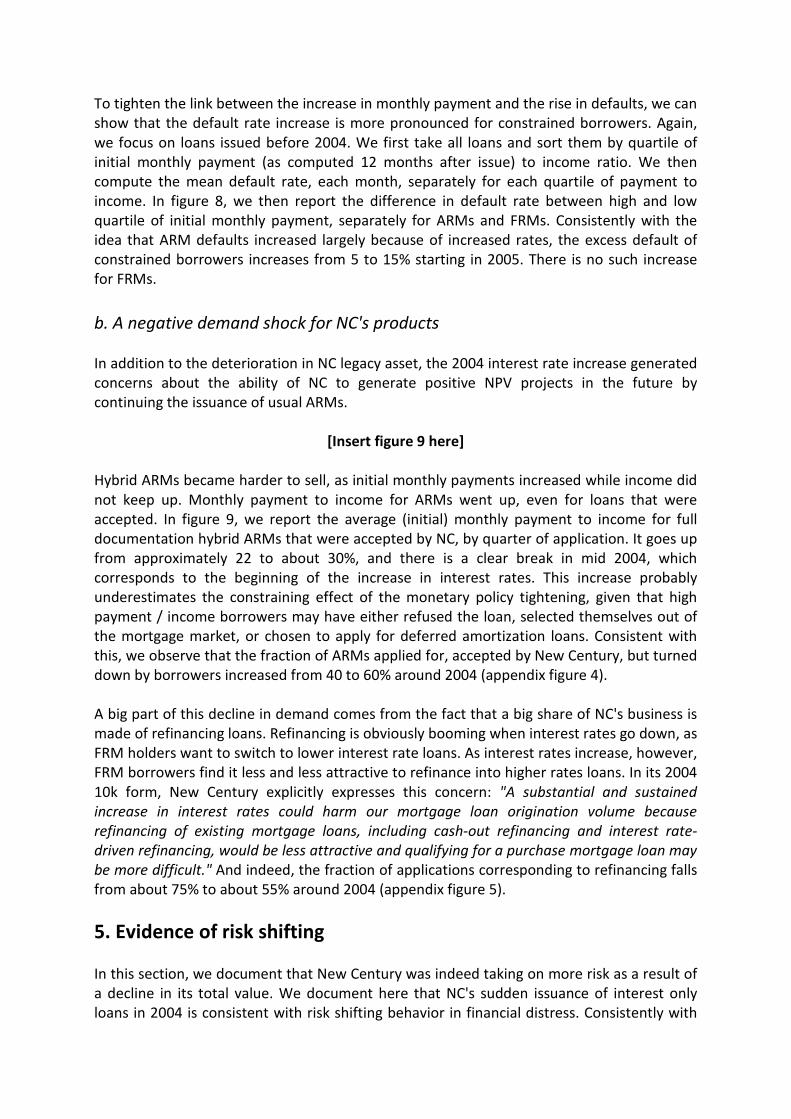
To tighten the link between the increase in monthly payment and the rise in defaults, we can show that the default rate increase is more pronounced for constrained borrowers. Again, we focus on loans issued before 2004. We first take all loans and sort them by quartile of initial monthly payment (as computed 12 months after issue) to income ratio. We then compute the mean default rate, each month, separately for each quartile of payment to income. In figure 8, we then report the difference in default rate between high and low quartile of initial monthly payment, separately for ARMs and FRMs. Consistently with the idea that ARM defaults increased largely because of increased rates, the excess default of constrained borrowers increases from 5 to 15% starting in 2005. There is no such increase for FRMs. b. A negative demand shock for NC's products In addition to the deterioration in NC legacy asset, the 2004 interest rate increase generated concerns about the ability of NC to generate positive NPV projects in the future by continuing the issuance of usual ARMs.

[Insert figure 9 here]

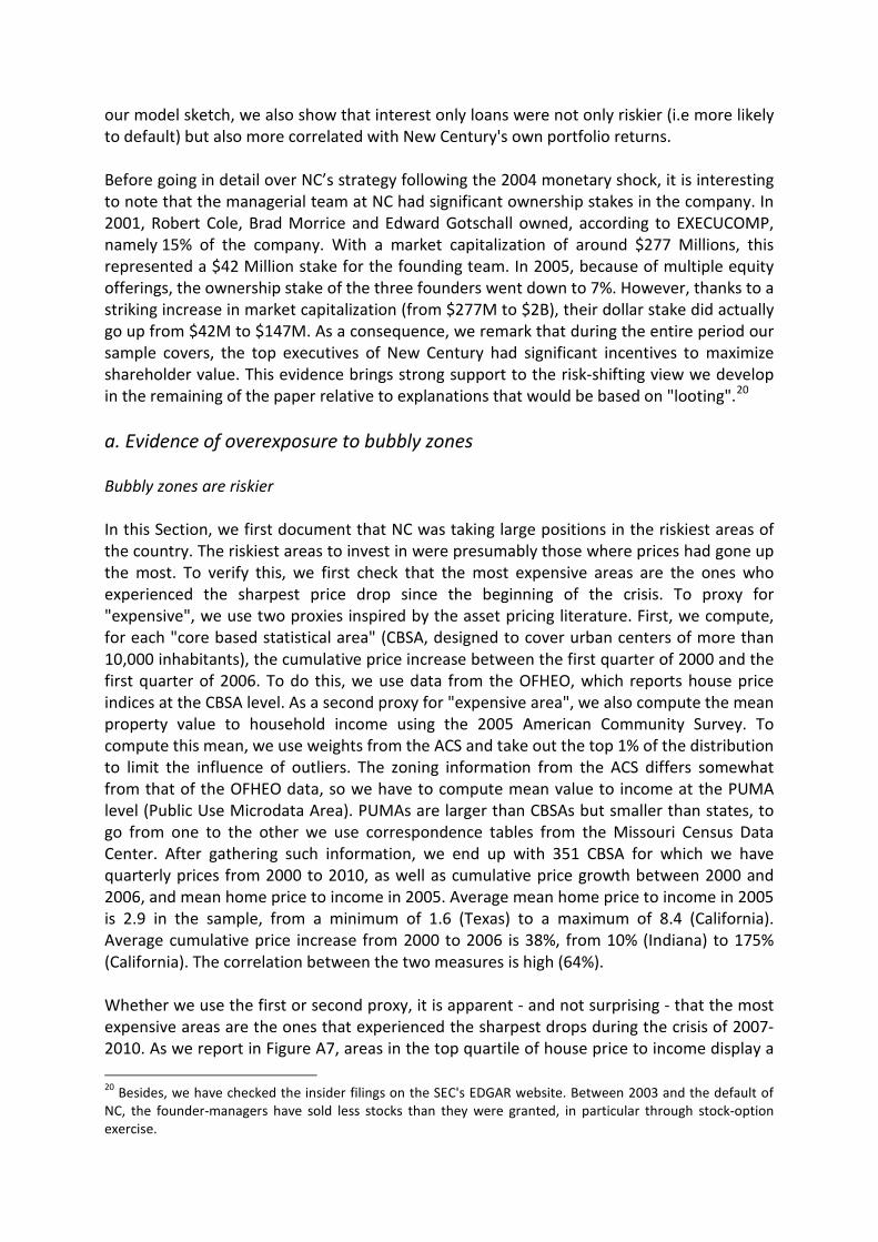
Hybrid ARMs became harder to sell, as initial monthly payments increased while income did not keep up. Monthly payment to income for ARMs went up, even for loans that were accepted. In figure 9, we report the average (initial) monthly payment to income for full documentation hybrid ARMs that were accepted by NC, by quarter of application. It goes up from approximately 22 to about 30%, and there is a clear break in mid 2004, which corresponds to the beginning of the increase in interest rates. This increase probably underestimates the constraining effect of the monetary policy tightening, given that high payment / income borrowers may have either refused the loan, selected themselves out of the mortgage market, or chosen to apply for deferred amortization loans. Consistent with this, we observe that the fraction of ARMs applied for, accepted by New Century, but turned down by borrowers increased from 40 to 60% around 2004 (appendix figure 4). A big part of this decline in demand comes from the fact that a big share of NC's business is made of refinancing loans. Refinancing is obviously booming when interest rates go down, as FRM holders want to switch to lower interest rate loans. As interest rates increase, however, FRM borrowers find it less and less attractive to refinance into higher rates loans. In its 2004 10k form, New Century explicitly expresses this concern: "A substantial and sustained increase in interest rates could harm our mortgage loan origination volume because refinancing of existing mortgage loans, including cash-out refinancing and interest rate-driven refinancing, would be less attractive and qualifying for a purchase mortgage loan may be more difficult." And indeed, the fraction of applications corresponding to refinancing falls from about 75% to about 55% around 2004 (appendix figure 5). 5. Evidence of risk shifting In this section, we document that New Century was indeed taking on more risk as a result of a decline in its total value. We document here that NC's sudden issuance of interest only loans in 2004 is consistent with risk shifting behavior in financial distress. Consistently with

our model sketch, we also show that interest only loans were not only riskier (i.e more likely to default) but also more correlated with New Century's own portfolio returns. Before going in detail over NC’s strategy following the 2004 monetary shock, it is interesting to note that the managerial team at NC had significant ownership stakes in the company. In 2001, Robert Cole, Brad Morrice and Edward Gotschall owned, according to EXECUCOMP, namely 15% of the company. With a market capitalization of around $277 Millions, this represented a $42 Million stake for the founding team. In 2005, because of multiple equity offerings, the ownership stake of the three founders went down to 7%. However, thanks to a striking increase in market capitalization (from $277M to $2B), their dollar stake did actually go up from $42M to $147M. As a consequence, we remark that during the entire period our sample covers, the top executives of New Century had significant incentives to maximize shareholder value. This evidence brings strong support to the risk-shifting view we develop in the remaining of the paper relative to explanations that would be based on "looting".20

a. Evidence of overexposure to bubbly zones Bubbly zones are riskier In this Section, we first document that NC was taking large positions in the riskiest areas of the country. The riskiest areas to invest in were presumably those where prices had gone up the most. To verify this, we first check that the most expensive areas are the ones who experienced the sharpest price drop since the beginning of the crisis. To proxy for "expensive", we use two proxies inspired by the asset pricing literature. First, we compute, for each "core based statistical area" (CBSA, designed to cover urban centers of more than 10,000 inhabitants), the cumulative price increase between the first quarter of 2000 and the first quarter of 2006. To do this, we use data from the OFHEO, which reports house price indices at the CBSA level. As a second proxy for "expensive area", we also compute the mean property value to household income using the 2005 American Community Survey. To compute this mean, we use weights from the ACS and take out the top 1% of the distribution to limit the influence of outliers. The zoning information from the ACS differs somewhat from that of the OFHEO data, so we have to compute mean value to income at the PUMA level (Public Use Microdata Area). PUMAs are larger than CBSAs but smaller than states, to go from one to the other we use correspondence tables from the Missouri Census Data Center. After gathering such information, we end up with 351 CBSA for which we have quarterly prices from 2000 to 2010, as well as cumulative price growth between 2000 and 2006, and mean home price to income in 2005. Average mean home price to income in 2005 is 2.9 in the sample, from a minimum of 1.6 (Texas) to a maximum of 8.4 (California). Average cumulative price increase from 2000 to 2006 is 38%, from 10% (Indiana) to 175% (California). The correlation between the two measures is high (64%). Whether we use the first or second proxy, it is apparent - and not surprising - that the most expensive areas are the ones that experienced the sharpest drops during the crisis of 2007-2010. As we report in Figure A7, areas in the top quartile of house price to income display a 20 Besides, we have checked the insider filings on the SEC's EDGAR website. Between 2003 and the default of NC, the founder-managers have sold less stocks than they were granted, in particular through stock-option exercise.

20% price drop over 2007-2010, while home prices are essentially flat in the other areas. In addition to being big, this difference is statistically significant, as shown in the regressions of Table A2. It is robust to excluding the three largest states in NC's activities: California, Texas and Florida. All in all, expensive, bubbly areas did indeed experience the sharpest price drop during the crisis. It is therefore reasonable to assume that lending in these areas in 2004 was presumably riskier than investing lending in cheaper areas. Post 2004, New Century invested more in bubbly areas We now report that NC biased its mortgage issuance in these expensive, risky, areas. To show this, we focus on the second one of our measures of bubbliness: property value to income (we do not report results using cumulative price growth to shorten exposition but there are qualitatively similar). Because we want to investigate NC's behavior starting in January 2004, we cannot use mean house price to income in 2005, as above. Instead, we measure here local average value to income using the 2000 census.21

[Insert table 7 about here] We then show that NC issued more loans in such "expensive" areas. For each of these areas, and for 2004, 2005 and 2006, we compute NC's total loan origination. We then regress local loan origination on our measure of area bubbliness. We report the result in Table 7, column 1. We find that indeed, loans issuance increase much more in expensive areas. This finding resists to the inclusion of several controls: In column 2, we control by the fraction of poor inhabitants, the fraction of college graduates (both from the 2000 census), and NC's total issuance in the area in 2003. The coefficient becomes smaller but remains significant at 1%: a 1 standard deviation increase in bubbliness (price to income increases by 4) leads to additional local issuance by about 40%. Last, in column 3, we control for land supply elasticity, which is an alternative proxy of home price volatility (Saiz, 2010, Chaney&al, 2010). We find that loan issue remains significantly correlated with our measure of bubbliness, but some of its effect is now captured by housing supply elasticity: NC lends more in less elastic, and therefore more volatile, areas after 2004. Post 2004, New Century leveraged its exposure to bubbly areas

[Insert figure 10 about here] An important issue that NC was facing in increasing its exposure to these areas was that, since houses were expensive relative incomes, too few borrowers would afford the monthly payment. To adjust to this, NC operated two levers: first, it lent to higher income borrowers, and second, it shifted to loans with lower monthly payment, i.e. interest-only loans. We have seen evidence of both behaviors in the descriptive section. What is more interesting is that both levers interacted: NC sold its new interest-only products to higher income people (on average, the monthly income of these recipients was $10K, as shown in Figure 10). Hence, NC was lending to richer borrowers who could afford a higher monthly payment, and

21 An alternative would be to take the 2003 American Community Survey. Unfortunately, the ACS microdata available from the web for 2001-2004 only provide state level geographic information. 2000 is the last year for which PUMA (i.e. more detailed) level information is available.

since these borrowers were initially not amortizing the principal of the loan, they could temporarily afford an even more expensive property.

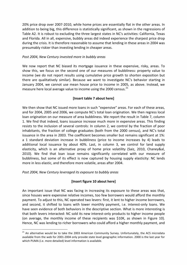
[Insert figure 11 about here] In Figure 11, we check graphically that interest-only products were aimed at expensive areas. To do this, we first sort zip codes by quartile average property value to income ratio (from 2000 census data). We then calculate the fraction of loans funded by New Century that are interest-only, or balloon loans, by month of application. We then plot the four lines, one per quartile of 2000 bubbliness. In the bottom quartile (highly affordable zip codes), the fraction of deferred amortization loans never reaches 20%. In the top quartile (highly expensive zip codes), the fraction of low amortization loans reaches 60% in 2006. Hence, deferred amortization loans (until 2005, these loans are interest-only loans only, balloons only appear in mid 2005) are aimed, in priority, at lending in expensive areas. We report the corresponding regression in Table 7, columns 4-9. In columns 4-6, we regress the local fraction of interest only loans issued on our measure of bubbliness and the same controls as in columns 1-3. It appears that bubbliness is a very strong correlate of interest-only diffusion. A 1 standard deviation increase in bubbliness (price to income ratio increase by 3) leads to an increase in the fraction of interest-only loans issued by about 10 ppt. It is highly significant and unaffected by controls. We also see (columns 7-9) that the propensity to lend to high income people (defined as the top quartile of the borrower income distribution in the sample) is increased by bubbliness (i.e. low affordability): A 1 standard deviation increase in bubbliness increases the percentage of high income by 15%. This is robust for controlling by the local fraction of high incomes among the 2003 borrowers. These results are unchanged in magnitude and significance when excluding California.

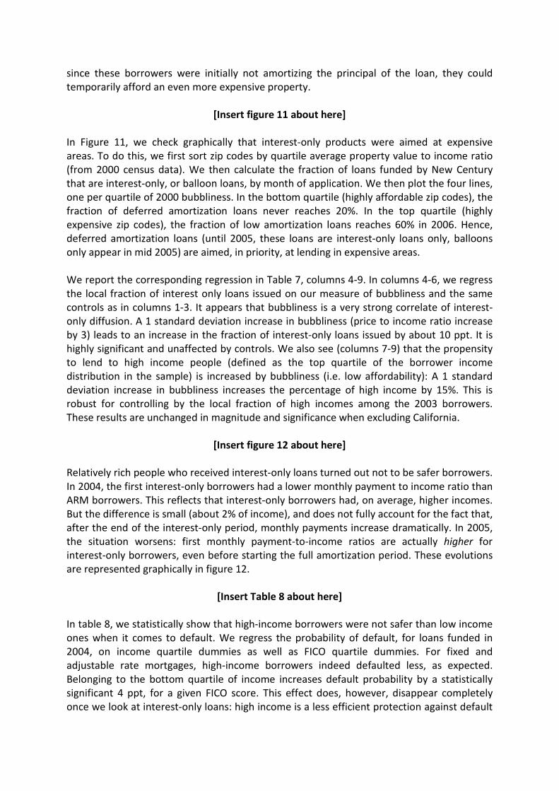
[Insert figure 12 about here] Relatively rich people who received interest-only loans turned out not to be safer borrowers. In 2004, the first interest-only borrowers had a lower monthly payment to income ratio than ARM borrowers. This reflects that interest-only borrowers had, on average, higher incomes. But the difference is small (about 2% of income), and does not fully account for the fact that, after the end of the interest-only period, monthly payments increase dramatically. In 2005, the situation worsens: first monthly payment-to-income ratios are actually higher for interest-only borrowers, even before starting the full amortization period. These evolutions are represented graphically in figure 12.

[Insert Table 8 about here] In table 8, we statistically show that high-income borrowers were not safer than low income ones when it comes to default. We regress the probability of default, for loans funded in 2004, on income quartile dummies as well as FICO quartile dummies. For fixed and adjustable rate mortgages, high-income borrowers indeed defaulted less, as expected. Belonging to the bottom quartile of income increases default probability by a statistically significant 4 ppt, for a given FICO score. This effect does, however, disappear completely once we look at interest-only loans: high income is a less efficient protection against default

for interest -only loans than for ARMs or FRMs. This comes from the fact that monthly payments were very high in interest-only loans. All in all, New Century started in 2004 to lend more aggressively in very expensive and hence risky areas. To make these loans affordable to its customer base, it moved toward richer households and since it was not enough, designed interest-only loans whose monthly payments were low enough. Moreover, these IO contracts were “bubble-riding” loans in the sense that, due to their very design, they were doomed to experience high default unless price growth remained high for the years following issuance. This is what we look at now in detail. b. Evidence from end of teaser period: the “sticker shock”.

[Insert figure 13 here] We first use the end of teaser period to identify the nature of risk inherent to interest-only loans. As seen above, these loans feature no amortization of the principal during the interest-only period, so the payment increase at the end of this period is bigger than for usual hybrid ARMs. Figure 13 provides visual evidence of this. For ARMs issued in 2004, the end of the teaser period occurred in 2006. Since interest rates increased a lot during this period, the monthly payment increase after the first reset was about 10-20% for these hybrids. For interest-only loans, this increase is on average larger than 50%: interest-only loans generate a huge "sticker shock" for borrowers.

[Insert figure 14 here]

This monthly payment shock after reset coincides with an increase in default. In figure 14, left panel, we plot the mean increase in monthly payment around reset for the three main categories of loans: ARMs, Interest-only and FRMs. FRMs are just a placebo here: they have no teaser period so we assume that these loans have their fictitious first reset 24 months after origination: logically enough, figure 14 shows that there is no increase in monthly payment after the end of the fictitious teaser period for FRMs. ARMs do, however, experience an increase in monthly payment. This increase is small to non-existent until 2004, which is expected since interest rates are stable and low until then. Then, following the increase in interest rates, the payment increase around reset goes to about 10%. The effect is much more dramatic for interest only loans, since the teaser rate was set during 2004, when rates were, overall, low. When the first interest-only loans reach the end of their interest-only period, monthly payment increases by about as much as 30%. These larger shocks were accompanied by a rise in defaults for these loans. In figure 14, right panel, we report the increase in default rate for loans around reset. For each loan around reset, we compute the difference between the mean default rate in the 6 months following reset, and the mean default rate in the 6 months before reset (consistent with the literature, a loan is said to default when payment is more than 60 days late). While the default increase around reset is stable for ARMs and FRMs, interest only loans experience a very sharp acceleration in post-reset default in early 2006. This sticker shock effect was a ticking bomb for the value of interest-only loans: absent an increase in properties value, borrowers were likely to find themselves unable to refinance or repay.

To connect monthly payment increase with default more directly, we also run the following regression:

where the LHS variable is a dummy equal to 1 if loan i defaults at date t (i.e. payment is more than 60 days late). The X's are loan-level controls: LTV, fico and year-of-origination dummy. POST is a dummy equal to 1 once the loan has passed the end of the teaser / interest-only period. We report results for interest-only and ARMs in Table 7 (columns 1 and 3, respectively). We find that the monthly probability of default increases by a significant 7.5 percentage points after the end of the teaser period for ARMs. The increase is larger for interest-only loans (9%), consistently with the idea that interest only loans trigger a much stronger payment shock around the first reset date. The differential increase between both types of loans is, however, insignificant.

[Insert table 9 here]

In addition to being riskier, we also expect returns on interest-only loans to be more sensitive to house prices. For constrained borrowers, once the reset date approaches, there are two options: either default, or refinance. In a phase of increasing interest rates, refinancing is more difficult, unless the value of the home had appreciated. If home value is higher, the borrower could use part of his new equity to lower interest rates. This is the principle behind lenders' points: a borrower can increase the face value of his debt - hence reduce his home equity - in exchange for a lower interest rate (Hall and Woodward, 2010). Hence, if real estate prices go up, it is possible for borrowers to refinance loans before the monthly payment explodes. This contention is borne out by the data: in table 7, columns 2 (for ARMs) and 4 (for interest-only), we report estimates of the following equation:

where LOWGROWTH is equal to 1 if home prices, as measured at the MSA level by the OFHEO, have grown by less than 10% between months t-12 and t. From this table iT appears that the increase in default rates for both ARMs and interest-only loans around reset are sensitive to real estate returns. This is consistent with the idea that these loans are risky and that their returns are low in states of nature where house prices grow little. Home price sensitivity is almost twice larger for interest only loans, which is consistent with the idea that the monthly payment shock around reset makes interest-only more likely to default when capital gains are too low to permit refinancing. Appendix figure 6, which plots month by month default rates around reset, confirms the intuition that interest-only are more price sensitive than ARMs: interest-only loans experience a cleaner break in default around reset, while defaults for ARMs just seem to drift continuously. Such behavior is consistent with our model sketch, which suggests that NC should tilt its portfolio towards assets that are more sensitive to its current portfolio's return. For a given

Defaultit = α + β.POSTit + Xi +ε it

Defaultit = α + β.POSTit × LOWGROWTHit + POSTit + LOWGROWTHit + Xi +ε it

loan granted, assuming New Century managers were maximizing equity value, they are indifferent to the payoffs of the loan in the scenario of bankruptcy (the bad state), while trying to maximize payoffs in the good sate. Thus, as the occurrence of the bad state was highly related to the burst of the real estate bubble, New Century must have been prone to adopt contractual features leading to high bankruptcy rates in the burst scenario, while yielding high payoffs in case of persistence of strong real estate prices. The contractual form of Interest Only loans was granting precisely that feature: when using such loans, borrowers are unlikely to be able to refinance unless prices keep growing, as the due payment jumps sharply at the reset date, where principal amortization starts. b. Evidence from unconditional default rates In this section, we check if the clean evidence that NC started to issue loans that are more price sensitive, gotten from focusing on the first reset date, carries to unconditional default rates. We first look at interest-only loans, and then look at richer, supposedly safer borrowers that were targeted in 2004. We argue that the default rates of these new loans were more elastic to real estate capital gains. Risk-shifting through contract design

Let us first establish a relatively high sensitivity of the cumulative default probability of interest-only loans to the drop in real estate prices. We focus on the 2004 vintage of loans granted by New Century, as it is the year where a large surge in IO contracts is observed. For each category of loan, we define a cumulative default dummy equal to one if the loan is ever observed to be more than sixty days delinquent over its lifecycle. We construct aggregate price measures at the zip code level (using MSA level information) and merge them to our servicing data. For each zip code where the price data are available, we construct each month the growth rate of prices over the two years following that month’s end. We defined quartiles of this growth rate using data for all available data over 1999 to 2005, which provides a discrete measure of relative price growth in a given zip code (the corresponding dummies are called “growth1”, “growth2”, “growth3”, “growth4”). We construct a second discrete measure of price growth: we say that there is slow growth in zip code i at month t if price growth in zip code i is lower than 10% for the 24 months following month t. We merge the zip code level data with our servicing data so that we have for each loan the measures of the growth of prices in the two years following the start of that loan’s life. There is a total of 21,828 loans for which we are able to get information on aggregate prices in their zipcode. 24% of these 2004 loans exhibit “slow growth” in local real estate prices during the 2 years following their start date. We then regress the cumulative default dummy defined above in loan level regressions (one observation per loan) where the right hand side variables is loan type (“FRM”, “ARM” and “IO”) interacted with the measures of price growth. The reference is “FRM” and in the quartile growth specification, the reference is “growth 1”, which corresponds to the lowest price growth quartile. We also control for the month of the loan’s start and in some

specifications for FICO and the Loan-to-Value ratio (LTV). Error terms are clustered at the date level (year and month of origination).

[Insert table 10 here]

The results, reported in table 8, show that IO loans exhibit a higher sensitivity of default to price growth: If prices stop growing fast, the implied increase in the probability of default is higher for an IO loan than for the two other types of loans. ARM loans also exhibit higher sensitivity of default to prices than ARM loans, but to a lesser extent than IO loans. The difference in sensitivity between IO and ARM loans is significant: for instance, in the first specification (column I), we can reject that the coefficient on “Slow Growth X IO” is equal to that on “Slow Growth X ARM” with a p-value of 2.1%. An IO loan is more likely to default when it is in a low growth zone by 8.5%, an economically significant amount (for IO loans, the average cumulative default probability is 12,8%). c. Evidence from loan selection In this last section, we test a more direct and specific implication of our simple risk-shifting model. We expect New Century to issue more IO loans in the areas that have a high beta with its own liabilities: high beta loans have high returns in states of nature where New Century is afloat (at the expense of low returns in states where New Century is bankrupt, and thus insensitive to). To compute this beta, we retrieve, for each MSA, the real estate annual price index starting in 1980 from OFHEO. We then call NCindex the aggregate index of MSA prices weighted by the amounts lent by NC in 2003. We see this index as a proxy for returns of New Century’s legacy asset and consider that New Century’s bankruptcy probability is largely determined by the performance of this asset. For each MSA, we compute the beta of local real estate prices with this NC index, using prices from 1980 till 2003. To test this specific risk-shifting hypothesis against alternatives, we also construct the betas of MSA level real estate prices on an equal-weighted real estate index (“beta_ewindex”) and on the growth of aggregate personal income (“beta_gincome”), which proxies for the returns of human capital (Source: Bureau of Economic Analysis, Table 2.1. Personal Income and Its Disposition). The betas are computed using yearly data between 1980 and 2003 (we stop in 2003 to eliminate any concern about a look-ahead bias). These betas have no particular reason (at least that we could think of) to affect portfolio selection; we view them more as placebos rather than as theoretically grounded controls.

[Insert table 11 here]

Because price indices are defined at the MSA level, we collapse the data by MSA-year and regress the percentage of each loan type (in each MSA-year) on the betas for loans originated in or after 2004. We have a total of 89 MSAs for which all our variables are defined. Results are reported in table 10, with t-stats clustered at the MSA level. We find, in line with our hypothesis, a strong and significant relationship between betas on the “legacy asset” and the propensity of New Century to issue Interest Only loans in a given MSA. This suggests that the accumulation of “bubble-riding” loans was primarily located in the MSAs

NC was highly sensitive to. We control for the MSA-level log of total amount lent in 2003, to be sure our results do not simply reflect that NC issues IO loans in zones where it has a higher presence. We also control for the local affordability, education and poverty measures based on the Census 2000, as well as the MSA-level total amount of loans originated in 2003. These results are robust to restricting the sample to non-Californian MSAs (see Appendix Table 1)). 6. Conclusion This paper has provided forensic evidence on the risk-shifting behavior of a large mortgage originator. The sharp rise in interest rate in 2004 destroyed a large fraction of New Century’s net present value. In reaction, New Century drastically modified its business model. It introduced a new, more price sensitive product: the interest-only loan. It changed its customer base, selling this new product to more credit-worthy, wealthier households, whose repayment decisions are also more sensitive to real estate prices. Finally, it changed the geography of its operations – selling more and more of these new loans in cities with real estate prices correlated with its legacy assets. This new business strategy is consistent with that of a financially distressed company that starts taking long bets on its own survival. Our paper has important implication for monetary policy. In response to a heating real estate market, policy makers thought in 2004 that increasing interest rates was the appropriate response. Our paper suggests this decision had dramatic consequences that were opposite to the effect sought out by the policy. By pushing mortgage originators closer to financial distress, the monetary policy tightening led mortgage originators to increase risk. In the case of New Century, risk taking took the form of a business that became much more sensitive to the continuation of the real estate bubble. All in all, this may well have fuelled the real estate bubble and eventually accentuate the burst of this bubble.

7. References Acharya, Schnabl and Suarez, 2010, "Securitization without risk transfer", working paper Almeida and Philippon, 2007, “The Risk-Adjusted Cost of Financial Distress”, Journal of Finance Akerlof and Romer, 1993, "Looting: the underworld of bankruptcy and profit", Brookings Papers on Economic Activity Andrade G. and Steven N Kaplan, 1998, “How costly is financial (not economic) distress? Evidence from highly leveraged transactions that became distressed”, The Journal of Finance, 53(5), pp. 1443-93. Barlevy and Fisher, 2010, "Mortgage choices and housing speculation", working paper Berndt, Hollifield and Sandas, 2009, "The role of mortgage brokers in the subprime crisis", NBER working paper Biais Bruno, Jean-Charles Rochet & Paul Woolley, 2010, “Innovations, rents and risk”, The Paul Woolley Centre, Working Paper Chaney, Sraer and Thesmar, 2010, "The collateral channel: How real estate prices affect investment", NBER WP 16060 Demyanyk and Van Hemert, 2009, "Understanding the subprime mortgage crisis", The Review of Financial Studies Demyanyk Yuliya and Otto Van Hemert, 2009, Understanding the Subprime Mortgage Crisis, Forthcoming the Review of Financial Studies. Diamond Doug., and Raghuram Rajan, 2009, "The Credit Crisis: Conjectures about Causes and Remedies," American Economic Review, May 2009. Esty, 1997, "A case study of organizational form and risk shifting in the savings and loans industry", Journal of Financial Economics Hall and Woodward, 2010, "Diagnosing consumer confusion and sub-optimal shopping effort: Theory and mortgage-market evidence", working paper Jiang, Nelson and Vytlacil, 2010, "Liar's loans? Effects of origination channel and information falsification on mortgage deliquency", Working paper Kashyap, Anil K., Raghuram G. Rajan, and Jeremy C. Stein. 2008. “Rethinking Capital Regulation.” Paper presented at the Maintaining Stability in a Changing Financial System Federal Reserve Bank of Kansas Symposium, Jackson Hole, WY.

Keys, Mukerjee, Seru and Vig, 2010, "Did securitization lead to lax screening? Evidence from subprime loans", Quarterly Journal of Economics LaPorta, Lopez-de-Silanes and Zamarripa, 2003, "Related lending", The Quarterly Journal of Economics Mayer Chris, Karen Pence, and Shane M. Sherlund, 2009, “The Rise in Mortgage Defaults”, Journal of Economic Perspectives. Mian and Sufi, 2009, "The consequence of mortgage credit expansion: Evidence from the US mortgage default crisis", Quarterly Journal of Economics Missal J. Michael, 2008, Final Report, Bankruptcy Court Examiner, United States Bankruptcy Court. Miller, M.H., Modigliani, F., 1966. “Some estimates of the cost of capital to the electric utility Industry”, 1954-57. American Economic Review 57. Nadauld and Weisbach, 2010, "Did securitization affect the cost of corporate debt", working paper Parker and Vissing-Jorgensen, 2009, "Who bears aggregate fluctuation and how?", AER P&P Piskorski, Tomasz and Alexei Tchistyi. 2007. “Optimal Mortgage Design.” Columbia Business School Working Paper Rajan, 2005, "Has financial development made the word riskier", working paper Saiz, 2010, "The geographic determinants of housing supply", forthcoming Quarterly Journal of Economics Sherlund, Shane. 2008. “The Past, Present, and Future of Subprime Mortgages.” Federal Reserve Board, September. Shleifer and Vishny, 2010, "Unstable banking", Journal of Financial Economics Stiglitz Joseph E. and Andrew Weiss, 1981, “Credit Rationing in Markets with Imperfect Information” The American Economic Review, Vol. 71, No. 3., pp. 393-410. Stiglitz Joseph E., 2010, “It is folly to place all our trust in the Fed”, The Financial Times, oct. 18, 2010. Yellen Janet, Oct. 2010, prepared remarks to the annual meeting of the National Association for Business Economics.

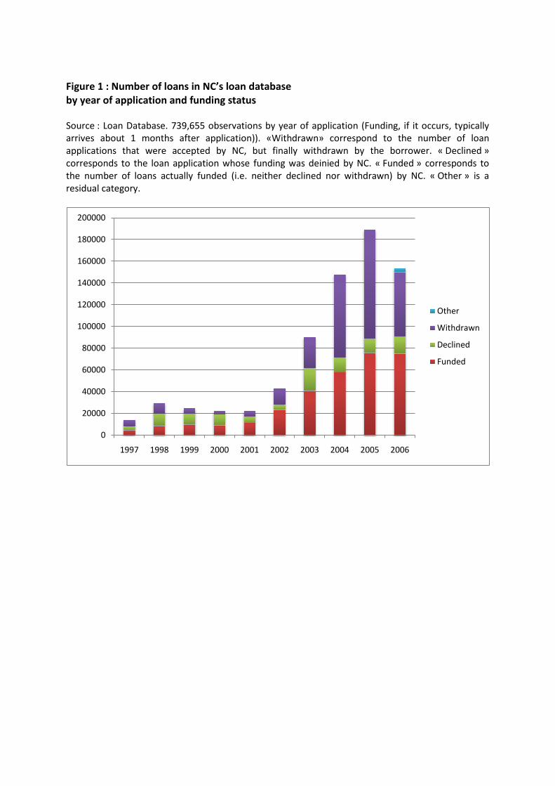
Figure 1 : Number of loans in NC’s loan database by year of application and funding status Source : Loan Database. 739,655 observations by year of application (Funding, if it occurs, typically arrives about 1 months after application)). «Withdrawn» correspond to the number of loan applications that were accepted by NC, but finally withdrawn by the borrower. « Declined » corresponds to the loan application whose funding was deinied by NC. « Funded » corresponds to the number of loans actually funded (i.e. neither declined nor withdrawn) by NC. « Other » is a residual category.

0

20000

40000

60000

80000

100000

120000

140000

160000

180000

200000

1997 1998 1999 2000 2001 2002 2003 2004 2005 2006

Other

Withdrawn

Declined

Funded

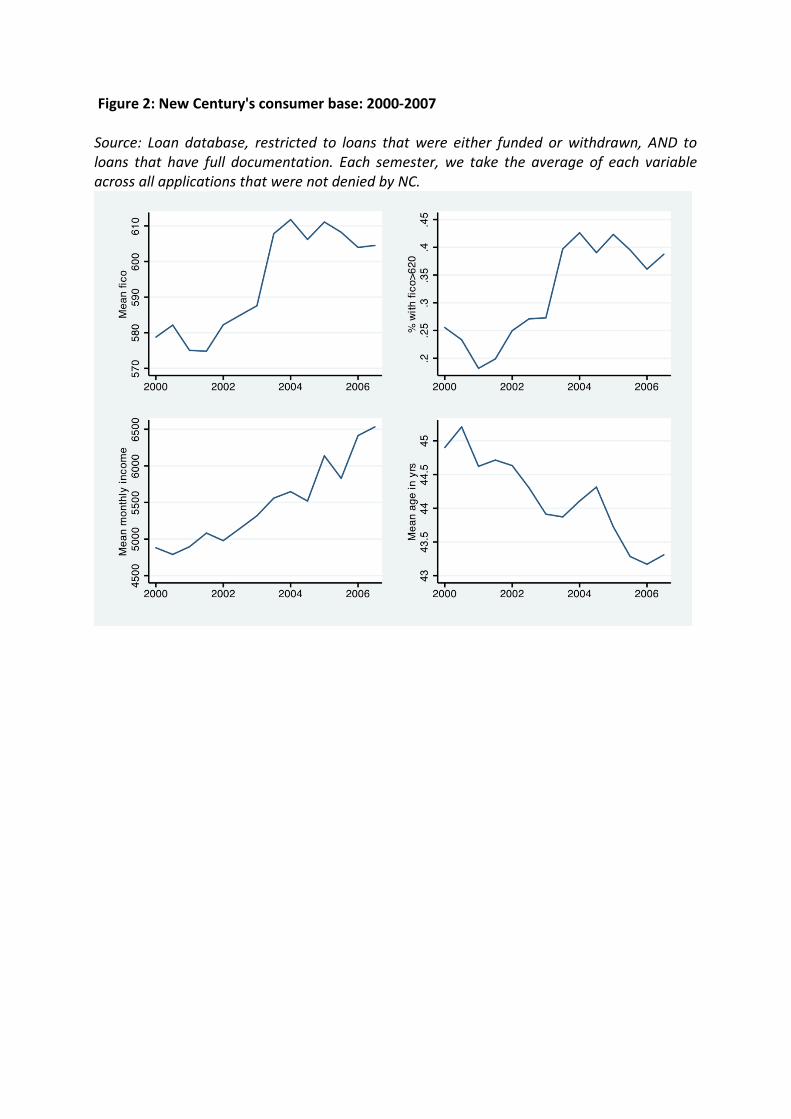
Figure 2: New Century's consumer base: 2000-2007 Source: Loan database, restricted to loans that were either funded or withdrawn, AND to loans that have full documentation. Each semester, we take the average of each variable across all applications that were not denied by NC.

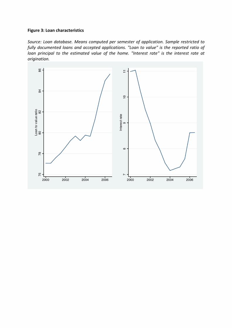
Figure 3: Loan characteristics Source: Loan database. Means computed per semester of application. Sample restricted to fully documented loans and accepted applications. "Loan to value" is the reported ratio of loan principal to the estimated value of the home. "Interest rate" is the interest rate at origination.

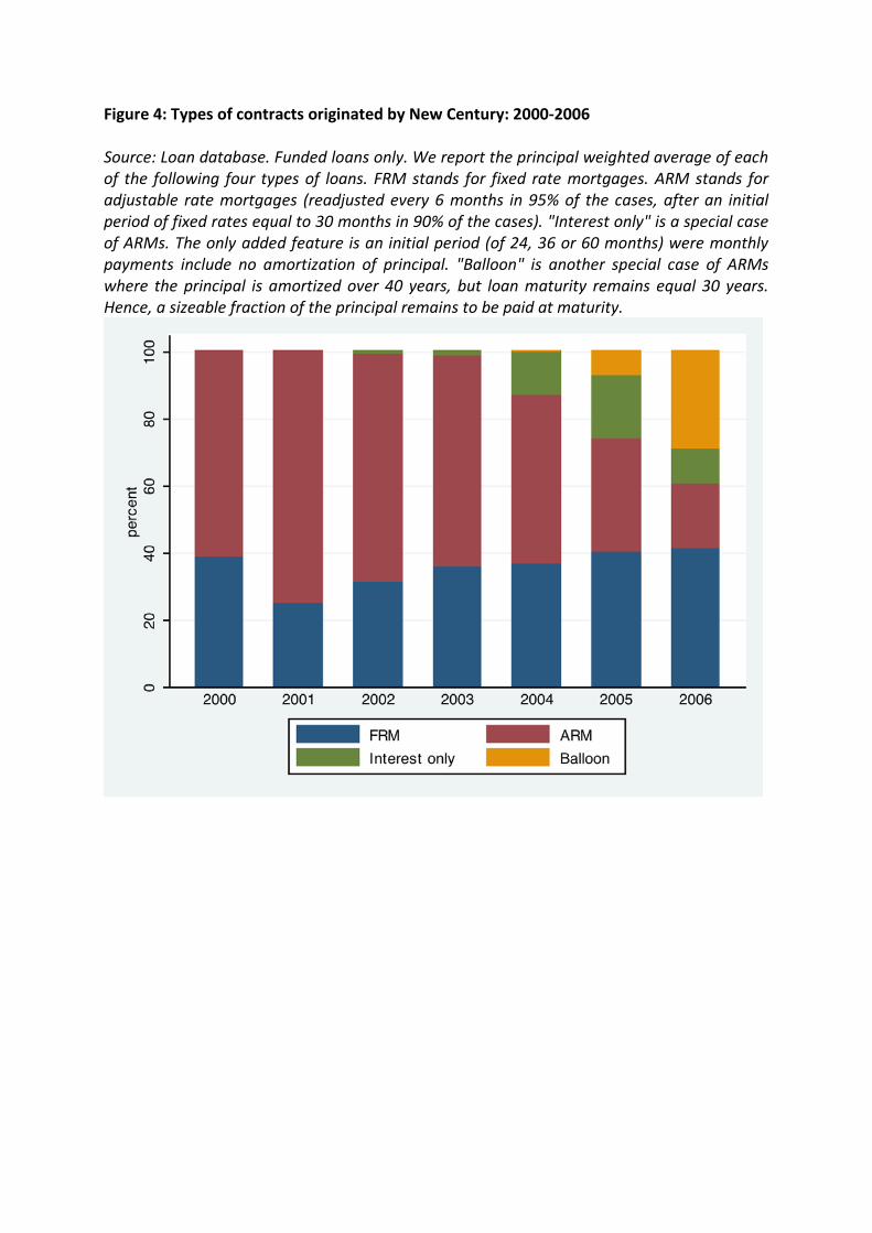
Figure 4: Types of contracts originated by New Century: 2000-2006 Source: Loan database. Funded loans only. We report the principal weighted average of each of the following four types of loans. FRM stands for fixed rate mortgages. ARM stands for adjustable rate mortgages (readjusted every 6 months in 95% of the cases, after an initial period of fixed rates equal to 30 months in 90% of the cases). "Interest only" is a special case of ARMs. The only added feature is an initial period (of 24, 36 or 60 months) were monthly payments include no amortization of principal. "Balloon" is another special case of ARMs where the principal is amortized over 40 years, but loan maturity remains equal 30 years. Hence, a sizeable fraction of the principal remains to be paid at maturity.

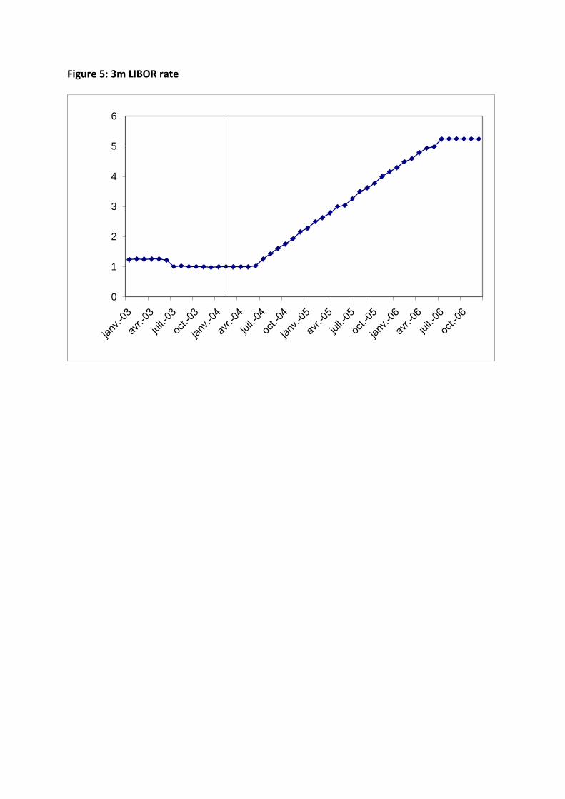
Figure 5: 3m LIBOR rate

0

1

2

3

4

5

6

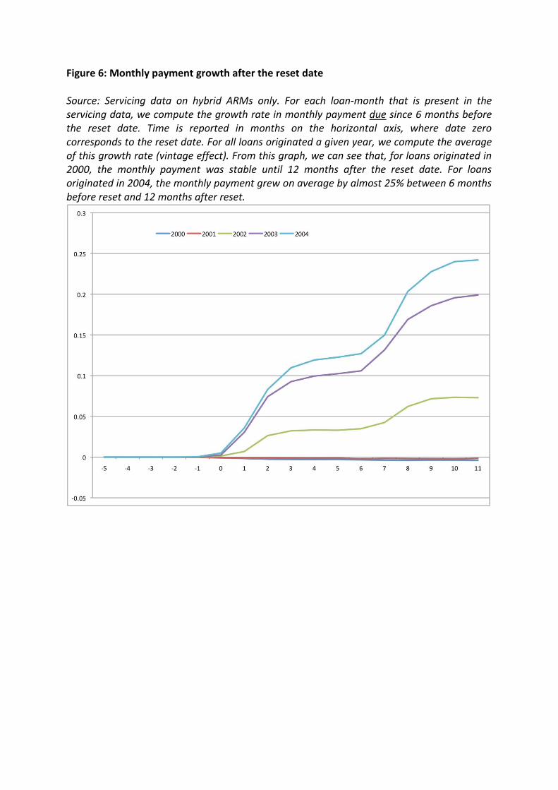
Figure 6: Monthly payment growth after the reset date Source: Servicing data on hybrid ARMs only. For each loan-month that is present in the servicing data, we compute the growth rate in monthly payment due since 6 months before the reset date. Time is reported in months on the horizontal axis, where date zero corresponds to the reset date. For all loans originated a given year, we compute the average of this growth rate (vintage effect). From this graph, we can see that, for loans originated in 2000, the monthly payment was stable until 12 months after the reset date. For loans originated in 2004, the monthly payment grew on average by almost 25% between 6 months before reset and 12 months after reset.

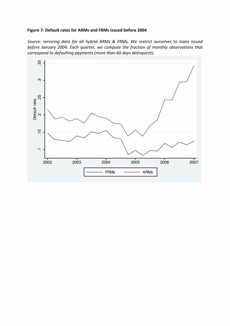
Figure 7: Default rates for ARMs and FRMs issued before 2004 Source: servicing data for all hybrid ARMs & FRMs. We restrict ourselves to loans issued before January 2004. Each quarter, we compute the fraction of monthly observations that correspond to defaulting payments (more than 60 days delinquent).

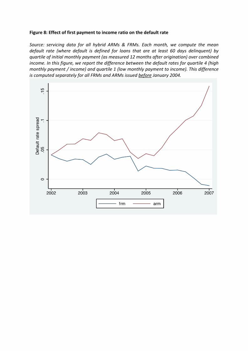
Figure 8: Effect of first payment to income ratio on the default rate Source: servicing data for all hybrid ARMs & FRMs. Each month, we compute the mean default rate (where default is defined for loans that are at least 60 days delinquent) by quartile of initial monthly payment (as measured 12 months after origination) over combined income. In this figure, we report the difference between the default rates for quartile 4 (high monthly payment / income) and quartile 1 (low monthly payment to income). This difference is computed separately for all FRMs and ARMs issued before January 2004.

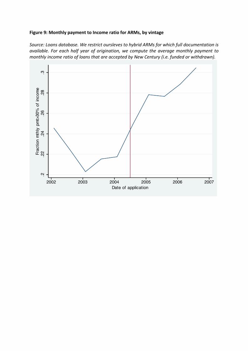
Figure 9: Monthly payment to Income ratio for ARMs, by vintage Source: Loans database. We restrict oursleves to hybrid ARMs for which full documentation is available. For each half year of origination, we compute the average monthly payment to monthly income ratio of loans that are accepted by New Century (i.e. funded or withdrawn).

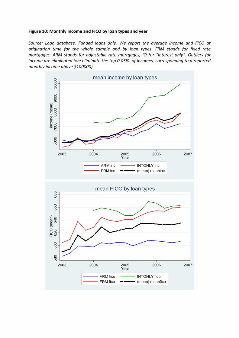
Figure 10: Monthly income and FICO by loan types and year Source: Loan database. Funded loans only. We report the average income and FICO at origination time for the whole sample and by loan types. FRM stands for fixed rate mortgages. ARM stands for adjustable rate mortgages, IO for "Interest only". Outliers for income are eliminated (we eliminate the top 0.05% of incomes, corresponding to a reported monthly income above $100000).

6000

7000

8000

9000

1000

0in

com

e (m

ean)

2003 2004 2005 2006 2007Year

ARM inc INTONLY incFRM inc (mean) meaninc

mean income by loan types

580

600

620

640

660

680

FIC

O (m

ean)

2003 2004 2005 2006 2007Year

ARM fico INTONLY ficoFRM fico (mean) meanfico

mean FICO by loan types

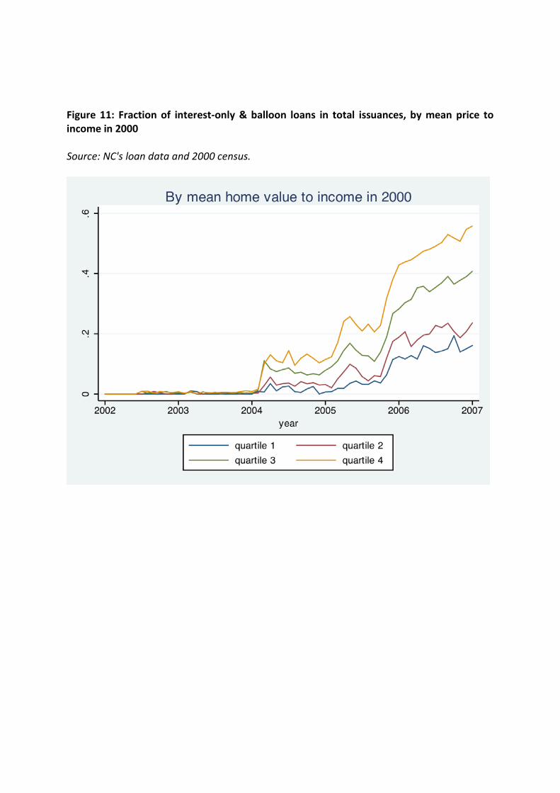
Figure 11: Fraction of interest-only & balloon loans in total issuances, by mean price to income in 2000 Source: NC's loan data and 2000 census.

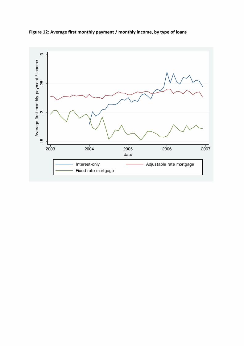
Figure 12: Average first monthly payment / monthly income, by type of loans

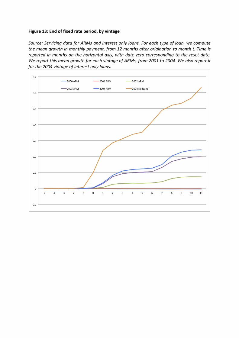
Figure 13: End of fixed rate period, by vintage Source: Servicing data for ARMs and interest only loans. For each type of loan, we compute the mean growth in monthly payment, from 12 months after origination to month t. Time is reported in months on the horizontal axis, with date zero corresponding to the reset date. We report this mean growth for each vintage of ARMs, from 2001 to 2004. We also report it for the 2004 vintage of interest only loans.

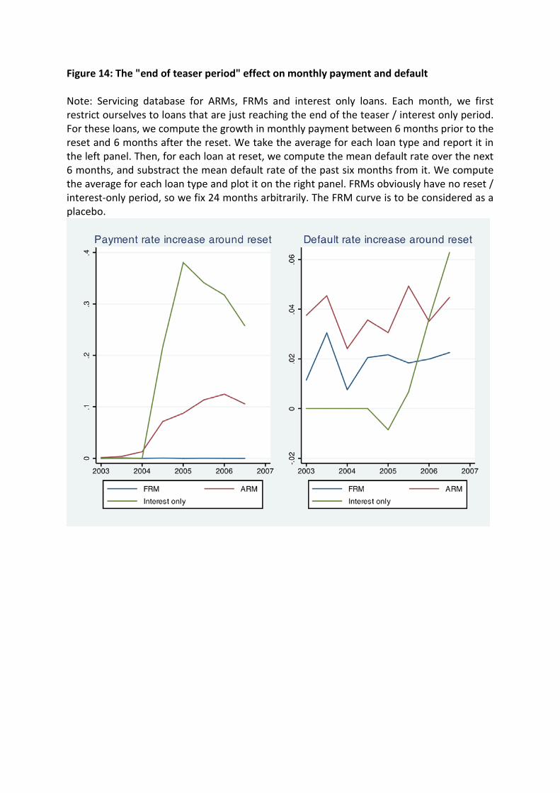
Figure 14: The "end of teaser period" effect on monthly payment and default Note: Servicing database for ARMs, FRMs and interest only loans. Each month, we first restrict ourselves to loans that are just reaching the end of the teaser / interest only period. For these loans, we compute the growth in monthly payment between 6 months prior to the reset and 6 months after the reset. We take the average for each loan type and report it in the left panel. Then, for each loan at reset, we compute the mean default rate over the next 6 months, and substract the mean default rate of the past six months from it. We compute the average for each loan type and plot it on the right panel. FRMs obviously have no reset / interest-only period, so we fix 24 months arbitrarily. The FRM curve is to be considered as a placebo.

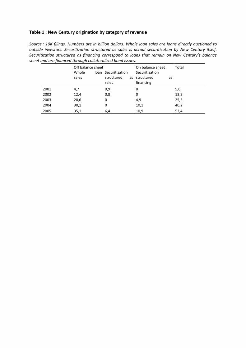
Table 1 : New Century origination by category of revenue Source : 10K filings. Numbers are in billion dollars. Whole loan sales are loans directly auctioned to outside investors. Securitization structured as sales is actual securitization by New Century itself. Securitization structured as financing correspond to loans that remain on New Century’s balance sheet and are financed through collateralized bond issues.

Off balance sheet On balance sheet Total

Whole loan sales

Securitization structured as sales

Securitization structured as financing

2001 4,7 0,9 0 5,6 2002 12,4 0,8 0 13,2 2003 20,6 0 4,9 25,5 2004 30,1 0 10,1 40,2 2005 35,1 6,4 10,9 52,4

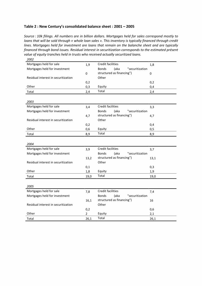
Table 2 : New Century’s consolidated balance sheet : 2001 – 2005 Source : 10k filings. All numbers are in billion dollars. Mortgages held for sales correspond mostly to loans that will be sold through « whole loan sales ». This inventory is typically financed through credit lines. Mortgages held for investment are loans that remain on the balanche sheet and are typically financed through bond issues. Residual interest in securitization corresponds to the estimated présent value of equity tranches held in trusts who received actually securitized loans.

2002 Mortgages held for sale 1,9 Credit facilities 1,8 Mortgages held for investment

0 Bonds (aka "securitization structured as financing") 0

Residual interest in securitization 0,2

Other 0,2

Other 0,3 Equity 0,4 Total 2,4 Total 2,4 2003 Mortgages held for sale 3,4 Credit facilities 3,3 Mortgages held for investment

4,7 Bonds (aka "securitization structured as financing") 4,7

Residual interest in securitization 0,2

Other 0,4

Other 0,6 Equity 0,5 Total 8,9 Total 8,9 2004 Mortgages held for sale 3,9 Credit facilities 3,7 Mortgages held for investment

13,2 Bonds (aka "securitization structured as financing") 13,1

Residual interest in securitization 0,1

Other 0,3

Other 1,8 Equity 1,9 Total 19,0 Total 19,0 2005 Mortgages held for sale 7,8 Credit facilities 7,4 Mortgages held for investment

16,1 Bonds (aka "securitization structured as financing") 16

Residual interest in securitization 0,2

Other 0,6

Other 2 Equity 2,1 Total 26,1 Total 26,1

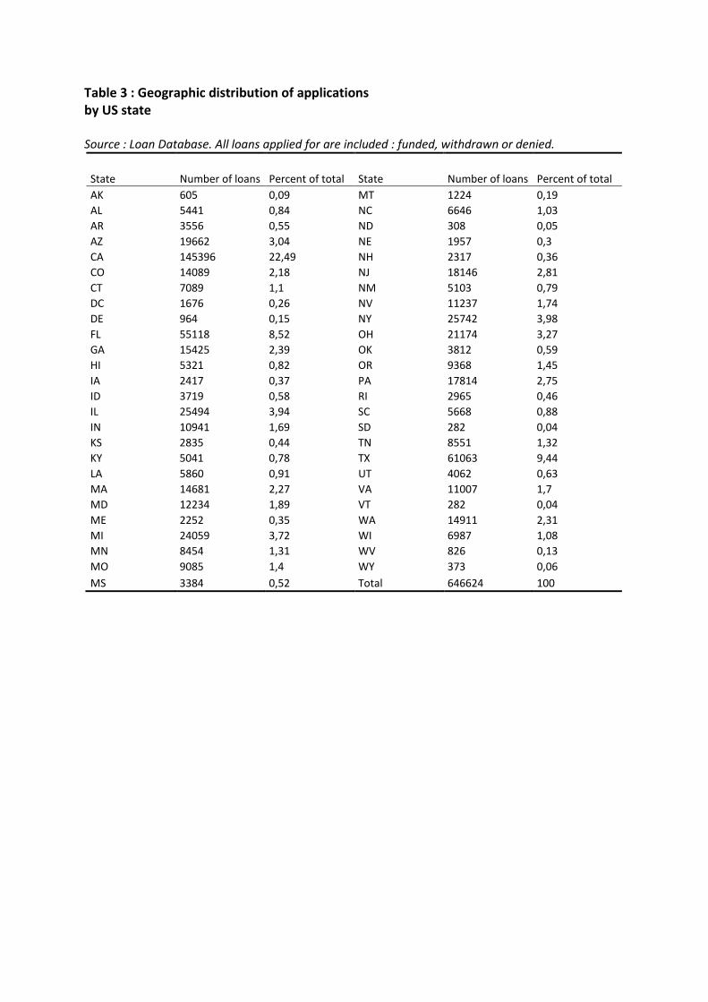
Table 3 : Geographic distribution of applications by US state Source : Loan Database. All loans applied for are included : funded, withdrawn or denied.

State Number of loans Percent of total State Number of loans Percent of total AK 605 0,09 MT 1224 0,19 AL 5441 0,84 NC 6646 1,03 AR 3556 0,55 ND 308 0,05 AZ 19662 3,04 NE 1957 0,3 CA 145396 22,49 NH 2317 0,36 CO 14089 2,18 NJ 18146 2,81 CT 7089 1,1 NM 5103 0,79 DC 1676 0,26 NV 11237 1,74 DE 964 0,15 NY 25742 3,98 FL 55118 8,52 OH 21174 3,27 GA 15425 2,39 OK 3812 0,59 HI 5321 0,82 OR 9368 1,45 IA 2417 0,37 PA 17814 2,75 ID 3719 0,58 RI 2965 0,46 IL 25494 3,94 SC 5668 0,88 IN 10941 1,69 SD 282 0,04 KS 2835 0,44 TN 8551 1,32 KY 5041 0,78 TX 61063 9,44 LA 5860 0,91 UT 4062 0,63 MA 14681 2,27 VA 11007 1,7 MD 12234 1,89 VT 282 0,04 ME 2252 0,35 WA 14911 2,31 MI 24059 3,72 WI 6987 1,08 MN 8454 1,31 WV 826 0,13 MO 9085 1,4 WY 373 0,06 MS 3384 0,52 Total 646624 100

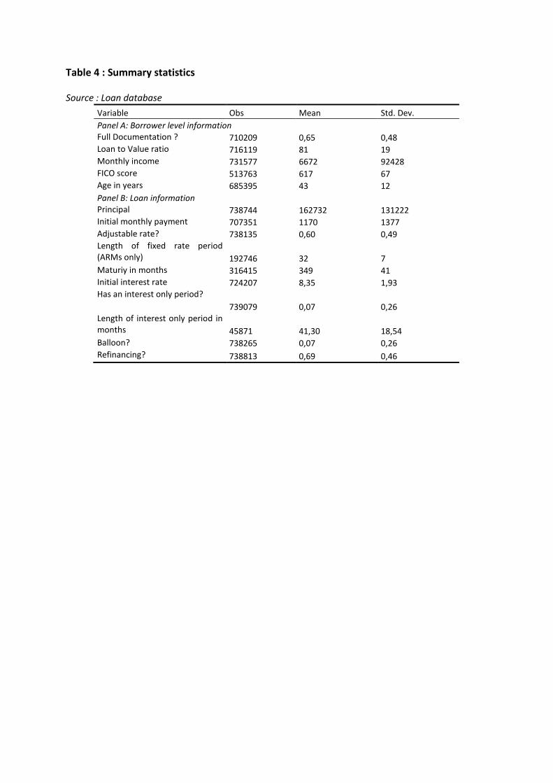
Table 4 : Summary statistics Source : Loan database

Variable Obs Mean Std. Dev. Panel A: Borrower level information Full Documentation ? 710209 0,65 0,48 Loan to Value ratio 716119 81 19 Monthly income 731577 6672 92428 FICO score 513763 617 67 Age in years 685395 43 12 Panel B: Loan information Principal 738744 162732 131222 Initial monthly payment 707351 1170 1377 Adjustable rate? 738135 0,60 0,49 Length of fixed rate period (ARMs only) 192746 32 7 Maturiy in months 316415 349 41 Initial interest rate 724207 8,35 1,93 Has an interest only period?

739079 0,07 0,26 Length of interest only period in months 45871 41,30 18,54 Balloon? 738265 0,07 0,26 Refinancing? 738813 0,69 0,46

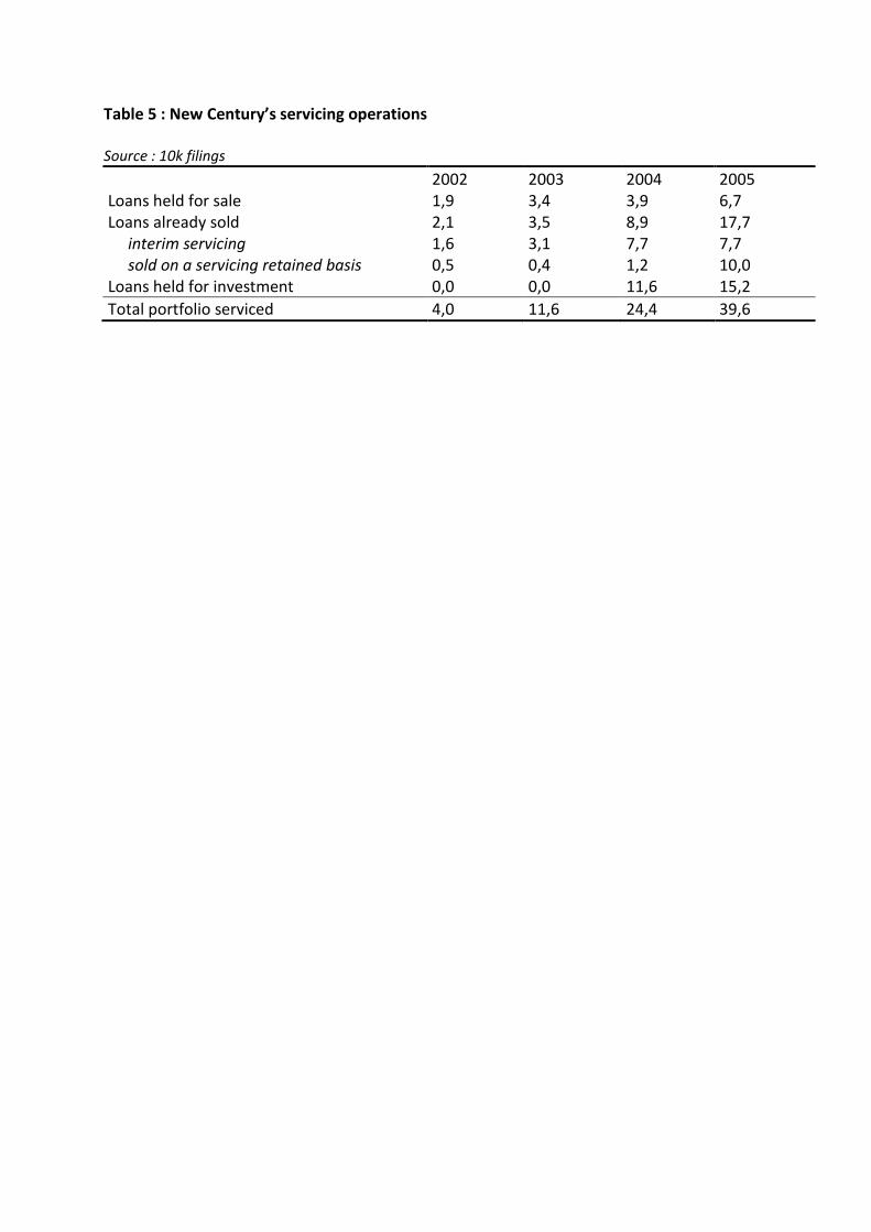
Table 5 : New Century’s servicing operations Source : 10k filings 2002 2003 2004 2005 Loans held for sale 1,9 3,4 3,9 6,7 Loans already sold 2,1 3,5 8,9 17,7 interim servicing 1,6 3,1 7,7 7,7 sold on a servicing retained basis 0,5 0,4 1,2 10,0 Loans held for investment 0,0 0,0 11,6 15,2 Total portfolio serviced 4,0 11,6 24,4 39,6

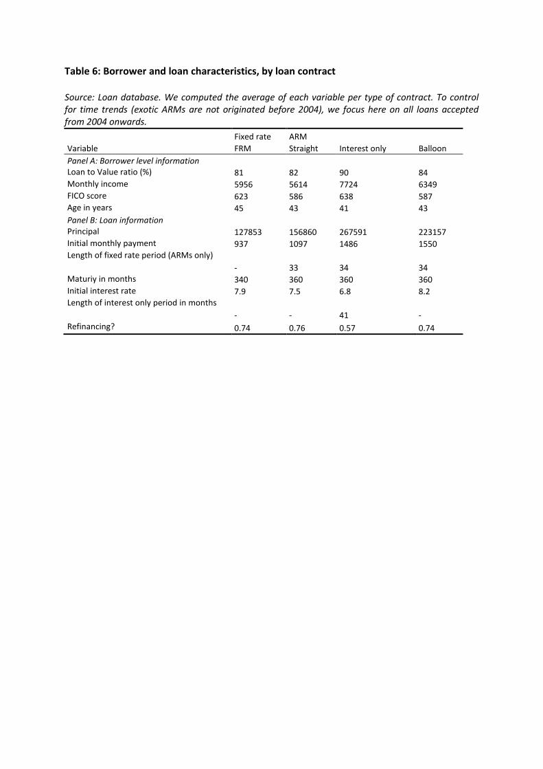
Table 6: Borrower and loan characteristics, by loan contract Source: Loan database. We computed the average of each variable per type of contract. To control for time trends (exotic ARMs are not originated before 2004), we focus here on all loans accepted from 2004 onwards. Fixed rate ARM Variable FRM Straight Interest only Balloon Panel A: Borrower level information Loan to Value ratio (%) 81 82 90 84 Monthly income 5956 5614 7724 6349 FICO score 623 586 638 587 Age in years 45 43 41 43 Panel B: Loan information Principal 127853 156860 267591 223157 Initial monthly payment 937 1097 1486 1550 Length of fixed rate period (ARMs only)

- 33 34 34 Maturiy in months 340 360 360 360 Initial interest rate 7.9 7.5 6.8 8.2 Length of interest only period in months

- - 41 - Refinancing? 0.74 0.76 0.57 0.74

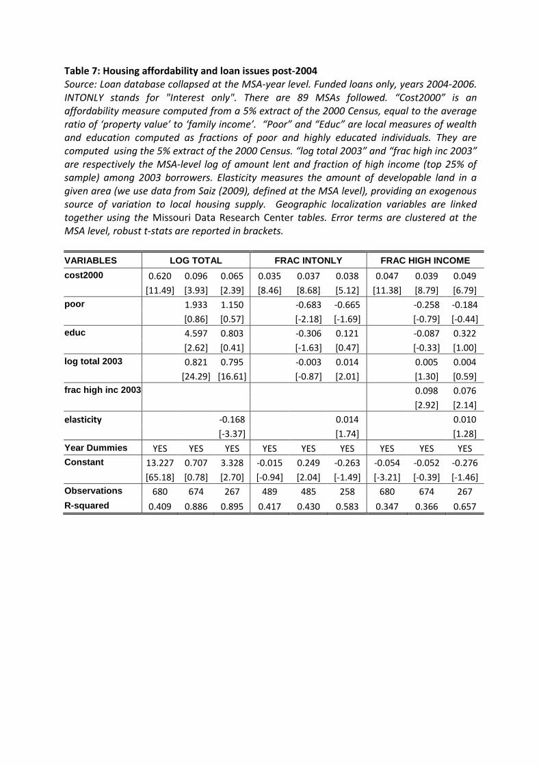
Table 7: Housing affordability and loan issues post-2004 Source: Loan database collapsed at the MSA-year level. Funded loans only, years 2004-2006. INTONLY stands for "Interest only". There are 89 MSAs followed. “Cost2000” is an affordability measure computed from a 5% extract of the 2000 Census, equal to the average ratio of ‘property value’ to ‘family income’. “Poor” and “Educ” are local measures of wealth and education computed as fractions of poor and highly educated individuals. They are computed using the 5% extract of the 2000 Census. “log total 2003” and “frac high inc 2003” are respectively the MSA-level log of amount lent and fraction of high income (top 25% of sample) among 2003 borrowers. Elasticity measures the amount of developable land in a given area (we use data from Saiz (2009), defined at the MSA level), providing an exogenous source of variation to local housing supply. Geographic localization variables are linked together using the Missouri Data Research Center tables. Error terms are clustered at the MSA level, robust t-stats are reported in brackets. VARIABLES LOG TOTAL FRAC INTONLY FRAC HIGH INCOME cost2000 0.620 0.096 0.065 0.035 0.037 0.038 0.047 0.039 0.049 [11.49] [3.93] [2.39] [8.46] [8.68] [5.12] [11.38] [8.79] [6.79] poor 1.933 1.150 -0.683 -0.665 -0.258 -0.184 [0.86] [0.57] [-2.18] [-1.69] [-0.79] [-0.44] educ 4.597 0.803 -0.306 0.121 -0.087 0.322 [2.62] [0.41] [-1.63] [0.47] [-0.33] [1.00] log total 2003 0.821 0.795 -0.003 0.014 0.005 0.004 [24.29] [16.61] [-0.87] [2.01] [1.30] [0.59] frac high inc 2003 0.098 0.076 [2.92] [2.14] elasticity -0.168 0.014 0.010 [-3.37] [1.74] [1.28] Year Dummies YES YES YES YES YES YES YES YES YES Constant 13.227 0.707 3.328 -0.015 0.249 -0.263 -0.054 -0.052 -0.276 [65.18] [0.78] [2.70] [-0.94] [2.04] [-1.49] [-3.21] [-0.39] [-1.46] Observations 680 674 267 489 485 258 680 674 267 R-squared 0.409 0.886 0.895 0.417 0.430 0.583 0.347 0.366 0.657

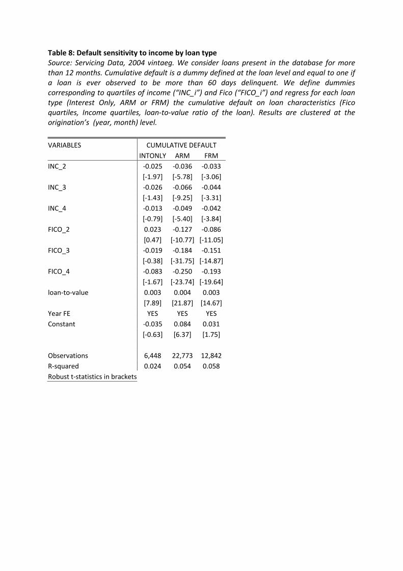
Table 8: Default sensitivity to income by loan type Source: Servicing Data, 2004 vintaeg. We consider loans present in the database for more than 12 months. Cumulative default is a dummy defined at the loan level and equal to one if a loan is ever observed to be more than 60 days delinquent. We define dummies corresponding to quartiles of income (“INC_i”) and Fico (“FICO_i”) and regress for each loan type (Interest Only, ARM or FRM) the cumulative default on loan characteristics (Fico quartiles, Income quartiles, loan-to-value ratio of the loan). Results are clustered at the origination’s (year, month) level. VARIABLES CUMULATIVE DEFAULT INTONLY ARM FRM INC_2 -0.025 -0.036 -0.033 [-1.97] [-5.78] [-3.06] INC_3 -0.026 -0.066 -0.044 [-1.43] [-9.25] [-3.31] INC_4 -0.013 -0.049 -0.042 [-0.79] [-5.40] [-3.84] FICO_2 0.023 -0.127 -0.086 [0.47] [-10.77] [-11.05] FICO_3 -0.019 -0.184 -0.151 [-0.38] [-31.75] [-14.87] FICO_4 -0.083 -0.250 -0.193 [-1.67] [-23.74] [-19.64] loan-to-value 0.003 0.004 0.003 [7.89] [21.87] [14.67] Year FE YES YES YES Constant -0.035 0.084 0.031 [-0.63] [6.37] [1.75] Observations 6,448 22,773 12,842 R-squared 0.024 0.054 0.058 Robust t-statistics in brackets

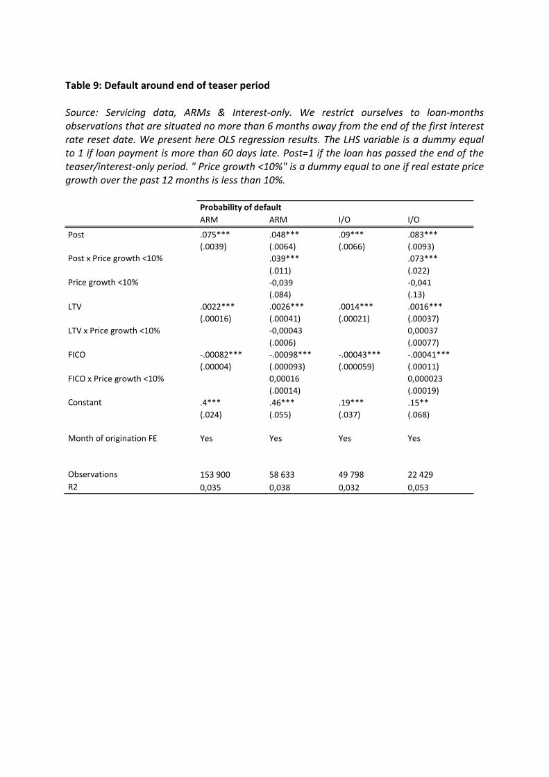
Table 9: Default around end of teaser period Source: Servicing data, ARMs & Interest-only. We restrict ourselves to loan-months observations that are situated no more than 6 months away from the end of the first interest rate reset date. We present here OLS regression results. The LHS variable is a dummy equal to 1 if loan payment is more than 60 days late. Post=1 if the loan has passed the end of the teaser/interest-only period. " Price growth <10%" is a dummy equal to one if real estate price growth over the past 12 months is less than 10%. Probability of default ARM ARM I/O I/O

Post .075*** .048*** .09*** .083*** (.0039) (.0064) (.0066) (.0093) Post x Price growth <10% .039*** .073*** (.011) (.022) Price growth <10% -0,039 -0,041 (.084) (.13) LTV .0022*** .0026*** .0014*** .0016*** (.00016) (.00041) (.00021) (.00037) LTV x Price growth <10% -0,00043 0,00037 (.0006) (.00077) FICO -.00082*** -.00098*** -.00043*** -.00041*** (.00004) (.000093) (.000059) (.00011) FICO x Price growth <10% 0,00016 0,000023 (.00014) (.00019) Constant .4*** .46*** .19*** .15** (.024) (.055) (.037) (.068) Month of origination FE Yes Yes Yes Yes Observations 153 900 58 633 49 798 22 429 R2 0,035 0,038 0,032 0,053

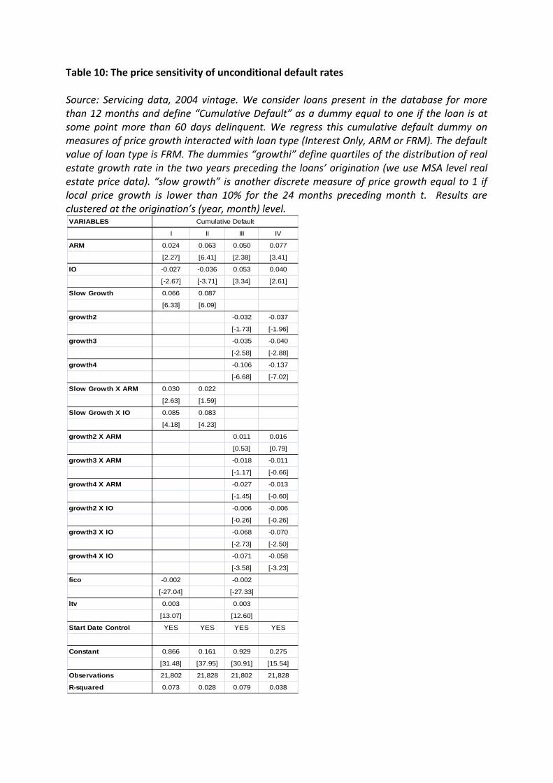
Table 10: The price sensitivity of unconditional default rates Source: Servicing data, 2004 vintage. We consider loans present in the database for more than 12 months and define “Cumulative Default” as a dummy equal to one if the loan is at some point more than 60 days delinquent. We regress this cumulative default dummy on measures of price growth interacted with loan type (Interest Only, ARM or FRM). The default value of loan type is FRM. The dummies “growthi” define quartiles of the distribution of real estate growth rate in the two years preceding the loans’ origination (we use MSA level real estate price data). “slow growth” is another discrete measure of price growth equal to 1 if local price growth is lower than 10% for the 24 months preceding month t. Results are clustered at the origination’s (year, month) level.

VARIABLES

I II III IV

ARM 0.024 0.063 0.050 0.077

[2.27] [6.41] [2.38] [3.41]

IO -0.027 -0.036 0.053 0.040

[-2.67] [-3.71] [3.34] [2.61]

Slow Growth 0.066 0.087

[6.33] [6.09]

growth2 -0.032 -0.037

[-1.73] [-1.96]

growth3 -0.035 -0.040

[-2.58] [-2.88]

growth4 -0.106 -0.137

[-6.68] [-7.02]

Slow Growth X ARM 0.030 0.022

[2.63] [1.59]

Slow Growth X IO 0.085 0.083

[4.18] [4.23]

growth2 X ARM 0.011 0.016

[0.53] [0.79]

growth3 X ARM -0.018 -0.011

[-1.17] [-0.66]

growth4 X ARM -0.027 -0.013

[-1.45] [-0.60]

growth2 X IO -0.006 -0.006

[-0.26] [-0.26]

growth3 X IO -0.068 -0.070

[-2.73] [-2.50]

growth4 X IO -0.071 -0.058

[-3.58] [-3.23]

fico -0.002 -0.002

[-27.04] [-27.33]

ltv 0.003 0.003

[13.07] [12.60]

Start Date Control YES YES YES YES

Constant 0.866 0.161 0.929 0.275

[31.48] [37.95] [30.91] [15.54]

Observations 21,802 21,828 21,802 21,828

R-squared 0.073 0.028 0.079 0.038

Cumulative Default

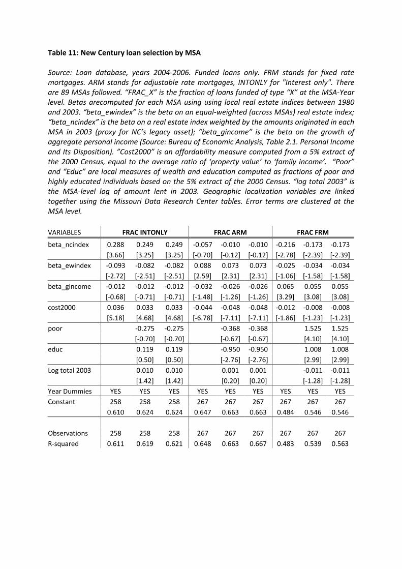
Table 11: New Century loan selection by MSA Source: Loan database, years 2004-2006. Funded loans only. FRM stands for fixed rate mortgages. ARM stands for adjustable rate mortgages, INTONLY for "Interest only". There are 89 MSAs followed. “FRAC_X” is the fraction of loans funded of type “X” at the MSA-Year level. Betas arecomputed for each MSA using using local real estate indices between 1980 and 2003. “beta_ewindex” is the beta on an equal-weighted (across MSAs) real estate index; “beta_ncindex” is the beta on a real estate index weighted by the amounts originated in each MSA in 2003 (proxy for NC’s legacy asset); “beta_gincome” is the beta on the growth of aggregate personal income (Source: Bureau of Economic Analysis, Table 2.1. Personal Income and Its Disposition). ”Cost2000” is an affordability measure computed from a 5% extract of the 2000 Census, equal to the average ratio of ‘property value’ to ‘family income’. “Poor” and “Educ” are local measures of wealth and education computed as fractions of poor and highly educated individuals based on the 5% extract of the 2000 Census. “log total 2003” is the MSA-level log of amount lent in 2003. Geographic localization variables are linked together using the Missouri Data Research Center tables. Error terms are clustered at the MSA level. VARIABLES FRAC INTONLY FRAC ARM FRAC FRM

beta_ncindex 0.288 0.249 0.249 -0.057 -0.010 -0.010 -0.216 -0.173 -0.173 [3.66] [3.25] [3.25] [-0.70] [-0.12] [-0.12] [-2.78] [-2.39] [-2.39] beta_ewindex -0.093 -0.082 -0.082 0.088 0.073 0.073 -0.025 -0.034 -0.034 [-2.72] [-2.51] [-2.51] [2.59] [2.31] [2.31] [-1.06] [-1.58] [-1.58] beta_gincome -0.012 -0.012 -0.012 -0.032 -0.026 -0.026 0.065 0.055 0.055 [-0.68] [-0.71] [-0.71] [-1.48] [-1.26] [-1.26] [3.29] [3.08] [3.08] cost2000 0.036 0.033 0.033 -0.044 -0.048 -0.048 -0.012 -0.008 -0.008 [5.18] [4.68] [4.68] [-6.78] [-7.11] [-7.11] [-1.86] [-1.23] [-1.23] poor -0.275 -0.275 -0.368 -0.368 1.525 1.525 [-0.70] [-0.70] [-0.67] [-0.67] [4.10] [4.10] educ 0.119 0.119 -0.950 -0.950 1.008 1.008 [0.50] [0.50] [-2.76] [-2.76] [2.99] [2.99] Log total 2003 0.010 0.010 0.001 0.001 -0.011 -0.011 [1.42] [1.42] [0.20] [0.20] [-1.28] [-1.28] Year Dummies YES YES YES YES YES YES YES YES YES Constant 258 258 258 267 267 267 267 267 267 0.610 0.624 0.624 0.647 0.663 0.663 0.484 0.546 0.546 Observations 258 258 258 267 267 267 267 267 267 R-squared 0.611 0.619 0.621 0.648 0.663 0.667 0.483 0.539 0.563

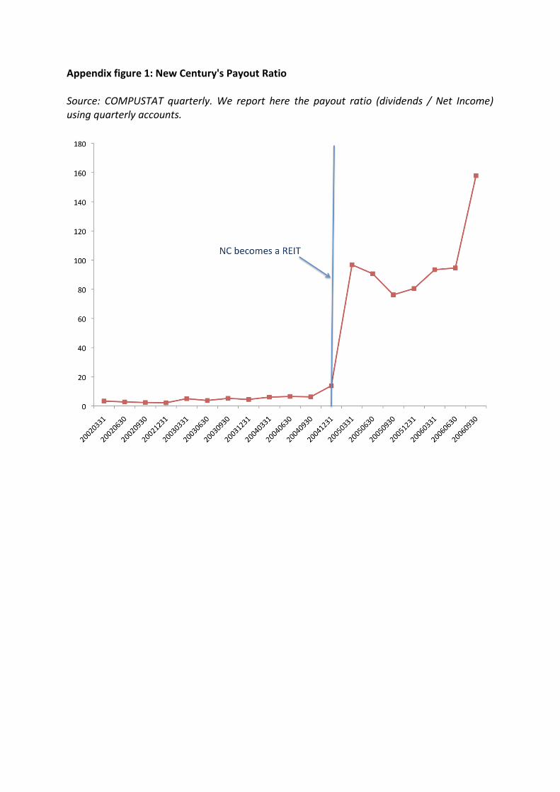
Appendix figure 1: New Century's Payout Ratio Source: COMPUSTAT quarterly. We report here the payout ratio (dividends / Net Income) using quarterly accounts.

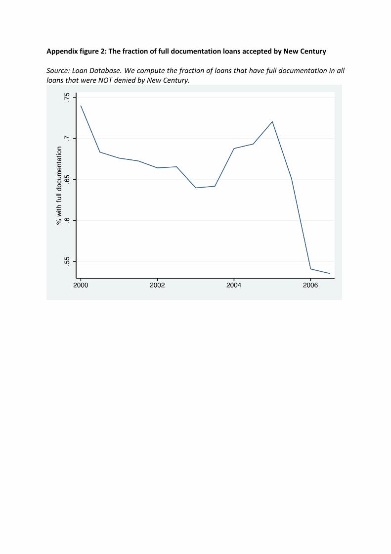
Appendix figure 2: The fraction of full documentation loans accepted by New Century Source: Loan Database. We compute the fraction of loans that have full documentation in all loans that were NOT denied by New Century.

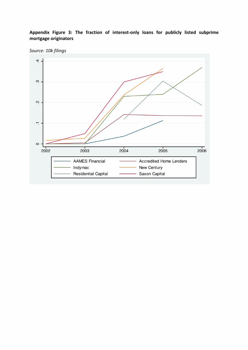
Appendix Figure 3: The fraction of interest-only loans for publicly listed subprime mortgage originators Source: 10k filings

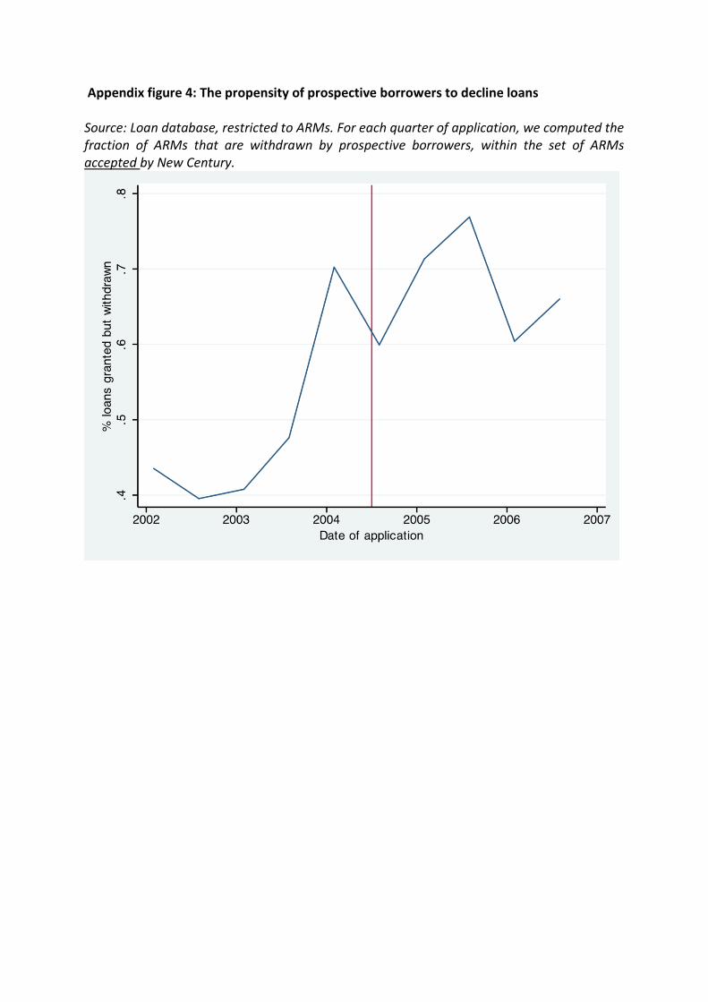
Appendix figure 4: The propensity of prospective borrowers to decline loans Source: Loan database, restricted to ARMs. For each quarter of application, we computed the fraction of ARMs that are withdrawn by prospective borrowers, within the set of ARMs accepted by New Century.

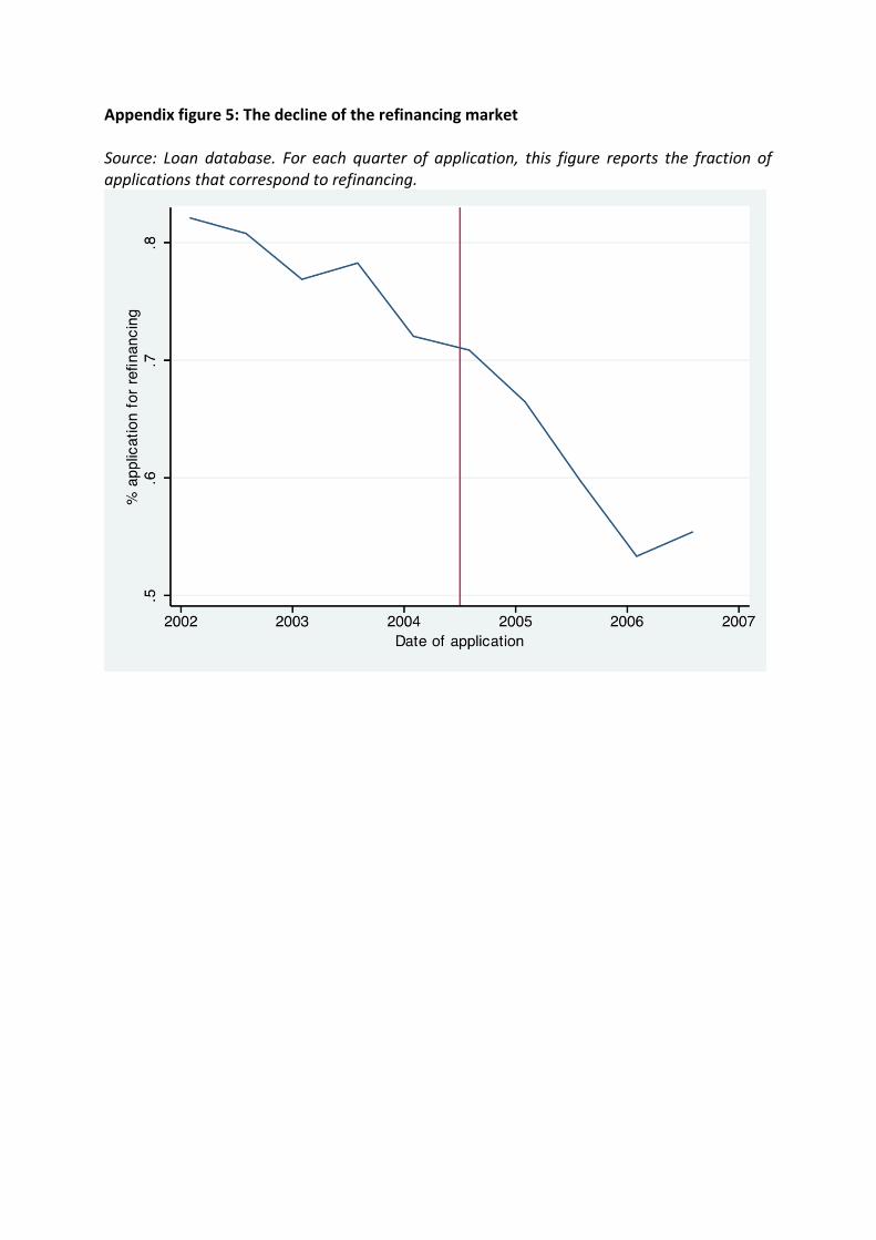
Appendix figure 5: The decline of the refinancing market Source: Loan database. For each quarter of application, this figure reports the fraction of applications that correspond to refinancing.

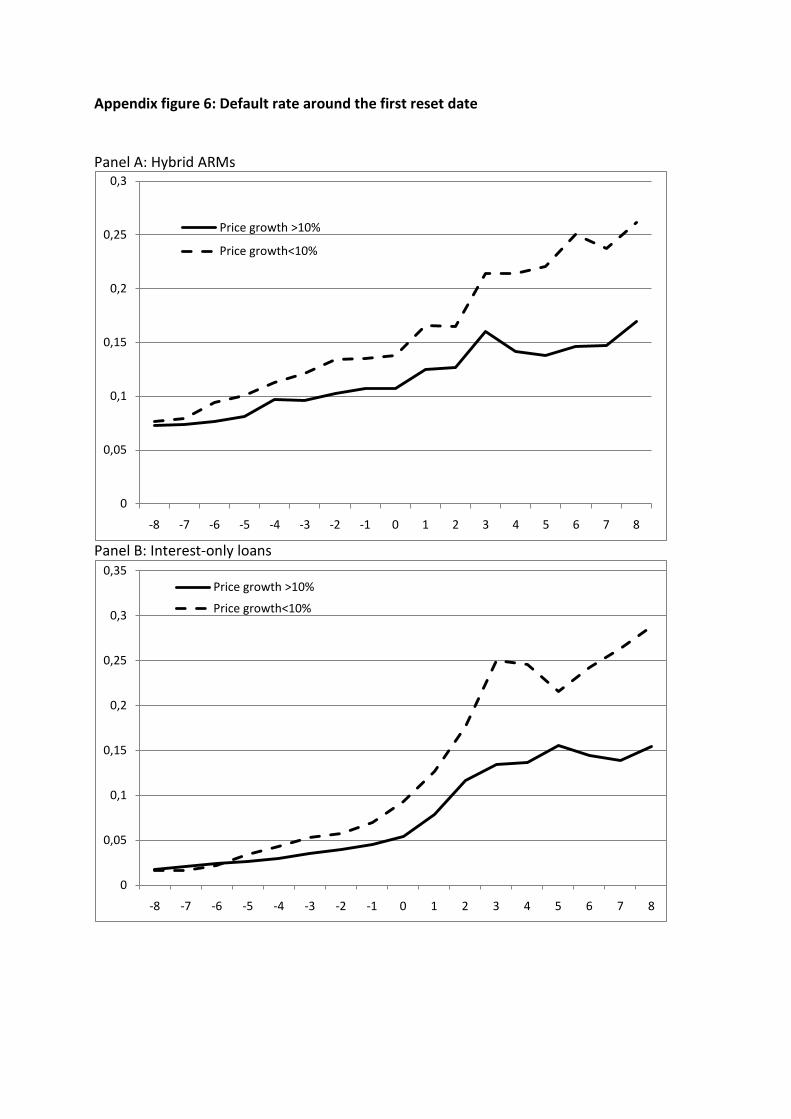
Appendix figure 6: Default rate around the first reset date Panel A: Hybrid ARMs

Panel B: Interest-only loans

0

0,05

0,1

0,15

0,2

0,25

0,3

-8 -7 -6 -5 -4 -3 -2 -1 0 1 2 3 4 5 6 7 8

Price growth >10%

Price growth<10%

0

0,05

0,1

0,15

0,2

0,25

0,3

0,35

-8 -7 -6 -5 -4 -3 -2 -1 0 1 2 3 4 5 6 7 8

Price growth >10%

Price growth<10%

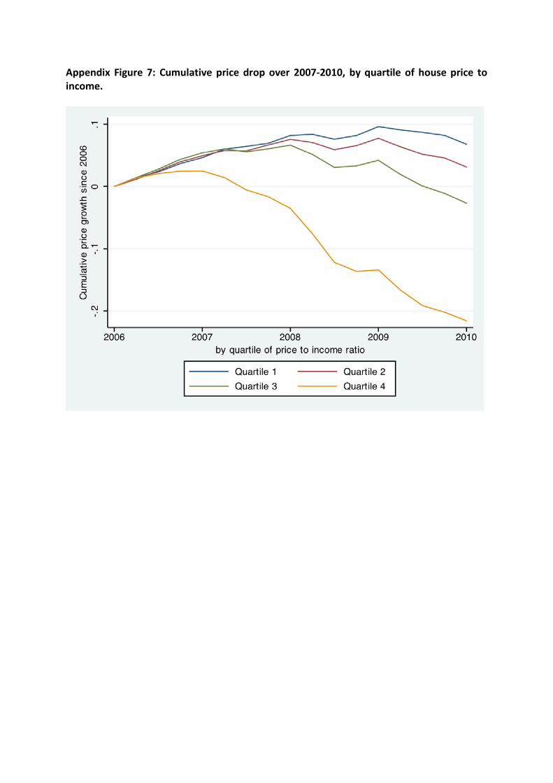
Appendix Figure 7: Cumulative price drop over 2007-2010, by quartile of house price to income.

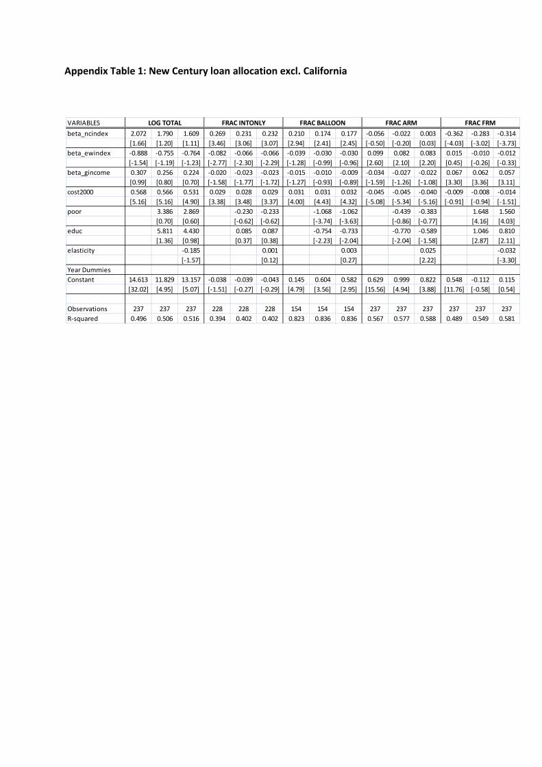
Appendix Table 1: New Century loan allocation excl. California

VARIABLESbeta_ncindex 2.072 1.790 1.609 0.269 0.231 0.232 0.210 0.174 0.177 -0.056 -0.022 0.003 -0.362 -0.283 -0.314

[1.66] [1.20] [1.11] [3.46] [3.06] [3.07] [2.94] [2.41] [2.45] [-0.50] [-0.20] [0.03] [-4.03] [-3.02] [-3.73]beta_ewindex -0.888 -0.755 -0.764 -0.082 -0.066 -0.066 -0.039 -0.030 -0.030 0.099 0.082 0.083 0.015 -0.010 -0.012

[-1.54] [-1.19] [-1.23] [-2.77] [-2.30] [-2.29] [-1.28] [-0.99] [-0.96] [2.60] [2.10] [2.20] [0.45] [-0.26] [-0.33]beta_gincome 0.307 0.256 0.224 -0.020 -0.023 -0.023 -0.015 -0.010 -0.009 -0.034 -0.027 -0.022 0.067 0.062 0.057

[0.99] [0.80] [0.70] [-1.58] [-1.77] [-1.72] [-1.27] [-0.93] [-0.89] [-1.59] [-1.26] [-1.08] [3.30] [3.36] [3.11]cost2000 0.568 0.566 0.531 0.029 0.028 0.029 0.031 0.031 0.032 -0.045 -0.045 -0.040 -0.009 -0.008 -0.014

[5.16] [5.16] [4.90] [3.38] [3.48] [3.37] [4.00] [4.43] [4.32] [-5.08] [-5.34] [-5.16] [-0.91] [-0.94] [-1.51]poor 3.386 2.869 -0.230 -0.233 -1.068 -1.062 -0.439 -0.383 1.648 1.560

[0.70] [0.60] [-0.62] [-0.62] [-3.74] [-3.63] [-0.86] [-0.77] [4.16] [4.03]educ 5.811 4.430 0.085 0.087 -0.754 -0.733 -0.770 -0.589 1.046 0.810

[1.36] [0.98] [0.37] [0.38] [-2.23] [-2.04] [-2.04] [-1.58] [2.87] [2.11]elasticity -0.185 0.001 0.003 0.025 -0.032

[-1.57] [0.12] [0.27] [2.22] [-3.30]Year DummiesConstant 14.613 11.829 13.157 -0.038 -0.039 -0.043 0.145 0.604 0.582 0.629 0.999 0.822 0.548 -0.112 0.115

[32.02] [4.95] [5.07] [-1.51] [-0.27] [-0.29] [4.79] [3.56] [2.95] [15.56] [4.94] [3.88] [11.76] [-0.58] [0.54]

Observations 237 237 237 228 228 228 154 154 154 237 237 237 237 237 237R-squared 0.496 0.506 0.516 0.394 0.402 0.402 0.823 0.836 0.836 0.567 0.577 0.588 0.489 0.549 0.581

LOG TOTAL FRAC INTONLY FRAC BALLOON FRAC ARM FRAC FRM

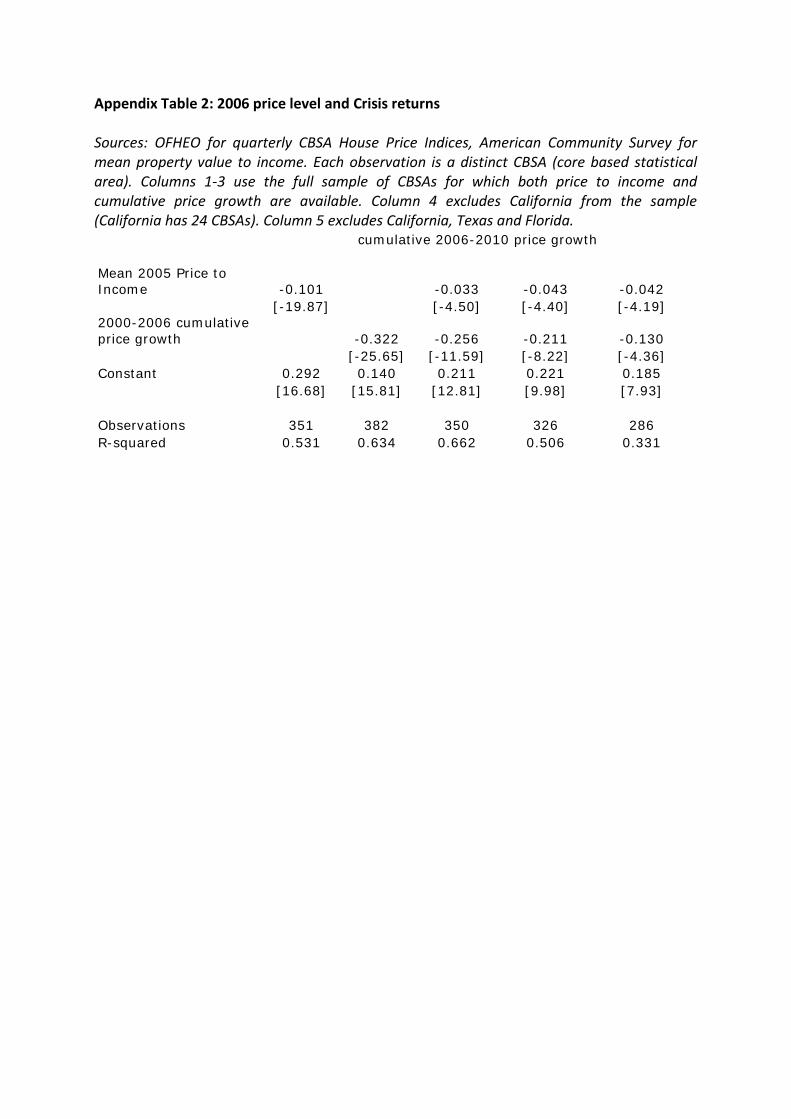
Appendix Table 2: 2006 price level and Crisis returns Sources: OFHEO for quarterly CBSA House Price Indices, American Community Survey for mean property value to income. Each observation is a distinct CBSA (core based statistical area). Columns 1-3 use the full sample of CBSAs for which both price to income and cumulative price growth are available. Column 4 excludes California from the sample (California has 24 CBSAs). Column 5 excludes California, Texas and Florida. cumulative 2006-2010 price growth Mean 2005 Price to Income -0.101 -0.033 -0.043 -0.042 [-19.87] [-4.50] [-4.40] [-4.19] 2000-2006 cumulative price growth -0.322 -0.256 -0.211 -0.130 [-25.65] [-11.59] [-8.22] [-4.36] Constant 0.292 0.140 0.211 0.221 0.185 [16.68] [15.81] [12.81] [9.98] [7.93] Observations 351 382 350 326 286 R-squared 0.531 0.634 0.662 0.506 0.331