Going towards the physical world

Till now, we have “played” with our images, and with our counts to extract the best possible instrumental magnitudes and positions.

A lot of work can be done with these measurements, but we have tokeep clear in mind that our fluxes are in some, totally arbitrary units.

A number of scientific applications need to have the stellar fluxes (or magnitudes) in some physical units.

Therefore, we need to calibrate (*) our instrumental magnitudes into some, properly defined photometric system.

(*) Note that the term “calibration” might generate some confusion. Someone uses theterm calibration to indicate the CCD pre-processing operations (bias, dark, flatfielding corrections). I personally prefer to use this term to indicate the complex operationsneeded to transform the instrumental magnitudes into a properly defined phot. system.

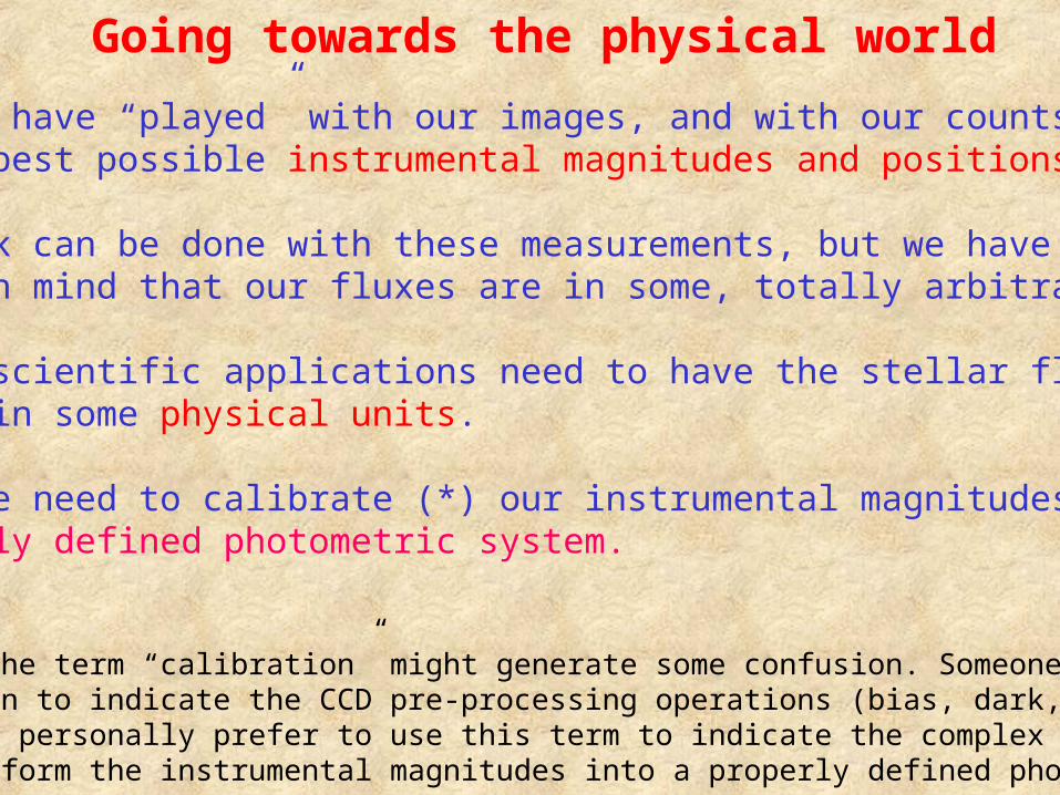
We need to matchphotometries fromdifferent observations/data sets:

1. For comparison;

2. Variability studies;

3. Extend magnitude/color coverage;

4. etc.

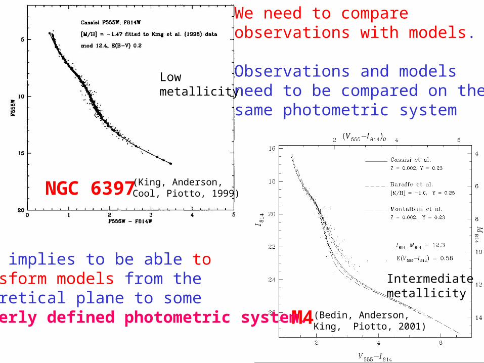
(Bedin, Anderson,King, Piotto, 2001)

NGC 6397

M4

(King, Anderson, Cool, Piotto, 1999)

We need to compareobservations with models.

Observations and modelsneed to be compared on thesame photometric system

Lowmetallicity

Intermediatemetallicity

This implies to be able to transform models from thetheoretical plane to someproperly defined photometric system.

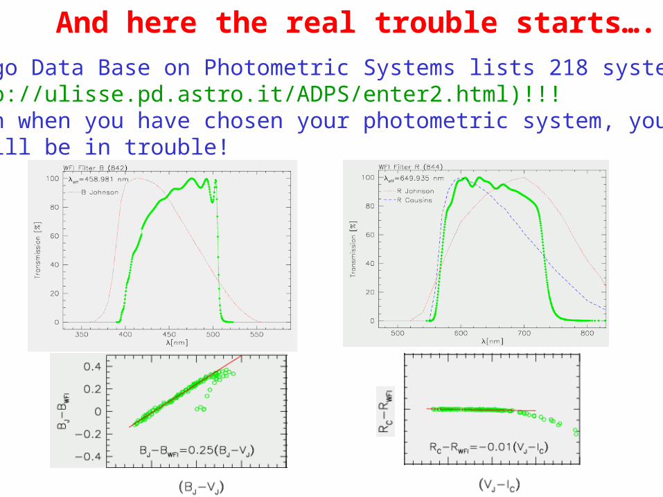
And here the real trouble starts….

The Asiago Data Base on Photometric Systems lists 218 systems (see http://ulisse.pd.astro.it/ADPS/enter2.html)!!!But, even when you have chosen your photometric system, youmight still be in trouble!

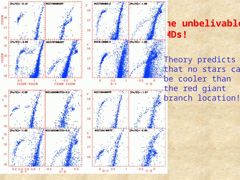
The unbelivable CMDs!

Theory predictsthat no stars can be cooler than the red giant branch location!

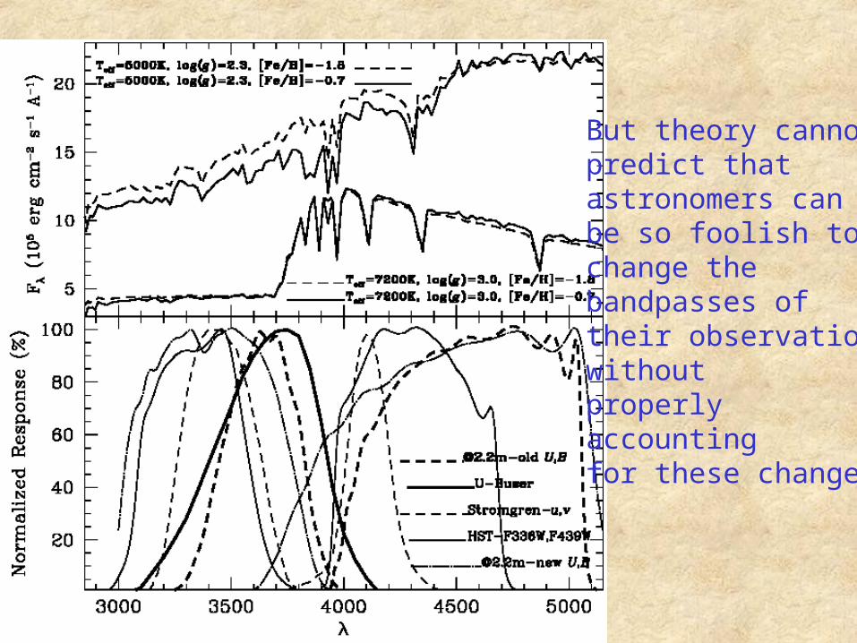
But theory cannotpredict thatastronomers can be so foolish tochange thebandpasses of their observationwithout properly accountingfor these changes

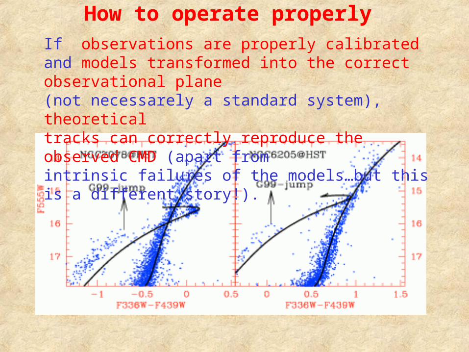
If observations are properly calibrated and models transformed into the correct observational plane(not necessarely a standard system), theoreticaltracks can correctly reproduce the observed CMD (apart fromintrinsic failures of the models…but this is a different story!).

How to operate properly

A general lesson

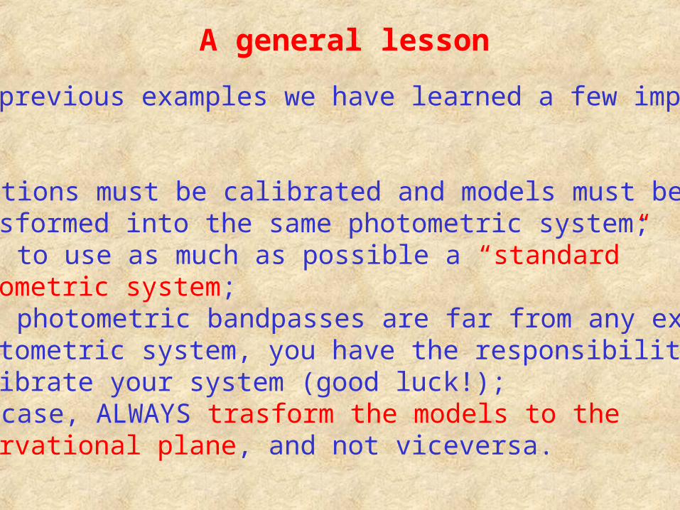
From the previous examples we have learned a few importantthings:

1. Observations must be calibrated and models must be transformed into the same photometric system;2. We need to use as much as possible a “standard” photometric system;3. If your photometric bandpasses are far from any existing photometric system, you have the responsibility to calibrate your system (good luck!);4. In any case, ALWAYS trasform the models to the observational plane, and not viceversa.

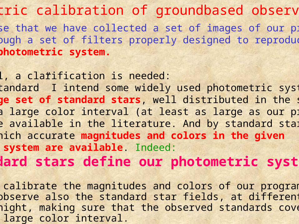
Photometric calibration of groundbased observationsLet’s suppose that we have collected a set of images of our program objects through a set of filters properly designed to reproduce a “standard” photometric system.

First of all, a clarification is needed: Here, by “standard” I intend some widely used photometric system forwhich a large set of standard stars, well distributed in the sky, andwhich span a large color interval (at least as large as our program objects) are available in the literature. And by standard stars I mean stars for which accurate magnitudes and colors in the given photometric system are available. Indeed:

the standard stars define our photometric system.

In order to calibrate the magnitudes and colors of our program objects,we need to observe also the standard star fields, at different timesduring the night, making sure that the observed standards cover a sufficently large color interval.

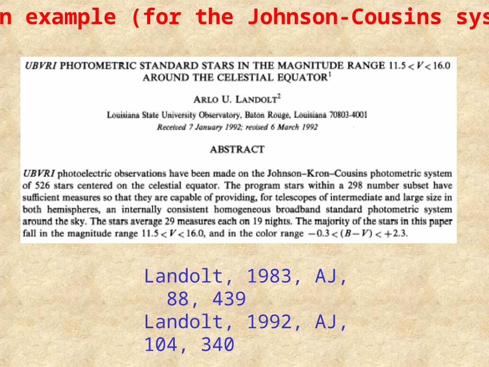
Just an example (for the Johnson-Cousins system):

Landolt, 1983, AJ, 88, 439Landolt, 1992, AJ, 104, 340

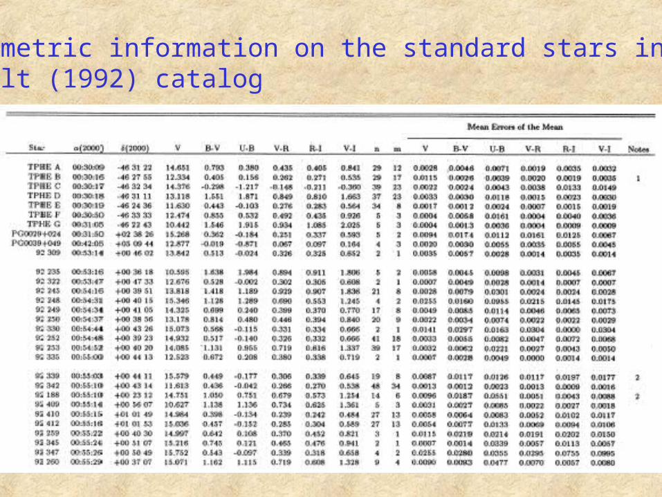
Photometric information on the standard stars in the Landolt (1992) catalog

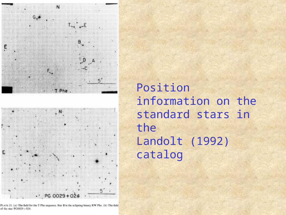
Position information on the standard stars in the Landolt (1992) catalog

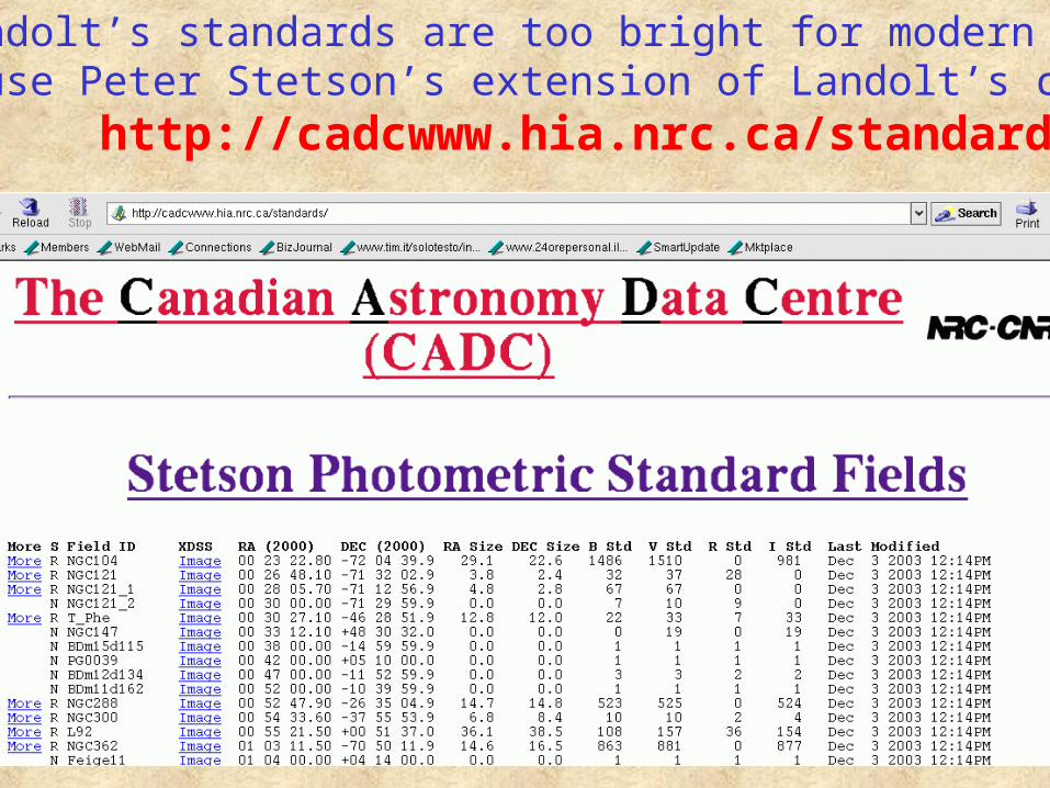
Most of Landolt’s standards are too bright for modern CCDs.Better to use Peter Stetson’s extension of Landolt’s catalog in: http://cadcwww.hia.nrc.ca/standards

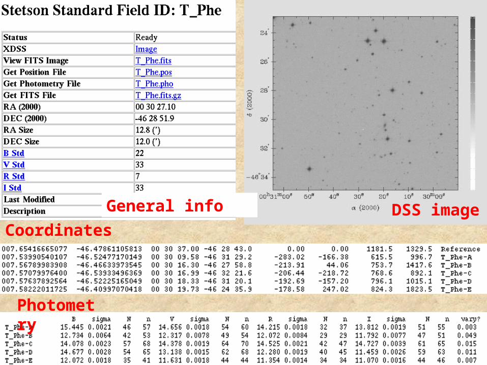
Coordinates

Photometry

DSS imageGeneral info

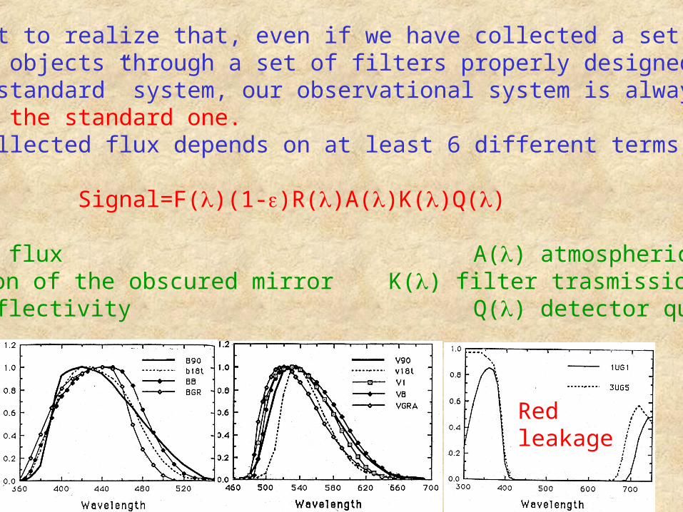
It is important to realize that, even if we have collected a set of images of our program objects through a set of filters properly designed to reproduce a “standard” system, our observational system is alwaysdifferent from the standard one.Indeed, the collected flux depends on at least 6 different terms:

Signal=F()(1-)R()A()K()Q()

F() incoming flux A() atmospheric absorption fraction of the obscured mirror K() filter trasmission curveR() mirror reflectivity Q() detector quantum efficency

Red leakage

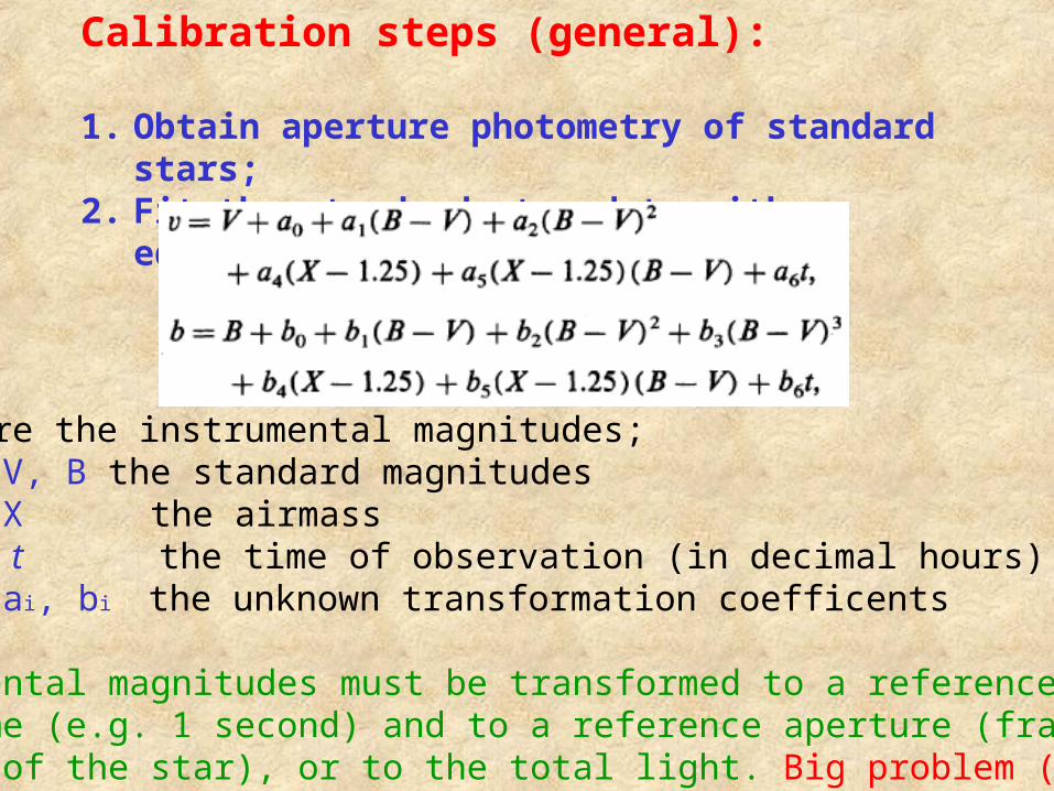
Calibration steps (general):

1. Obtain aperture photometry of standard stars;2. Fit the standard star data with equations of the type:

Where: v, b are the instrumental magnitudes; V, B the standard magnitudes X the airmass t the time of observation (in decimal hours) ai, bi the unknown transformation coefficents

The instrumental magnitudes must be transformed to a referenceexposure time (e.g. 1 second) and to a reference aperture (fraction oftotal light of the star), or to the total light. Big problem (see later)!

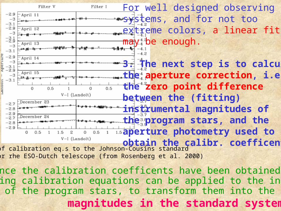
For well designed observingsystems, and for not too extreme colors, a linear fit may be enough.

3. The next step is to calculatethe aperture correction, i.e. the zero point difference between the (fitting)instrumental magnitudes ofthe program stars, and the aperture photometry used to obtain the calibr. coefficents.

Finally, once the calibration coefficents have been obtained, the corresponding calibration equations can be applied to the instrumental magnitudes of the program stars, to transform them into the beloved magnitudes in the standard system!

Example of calibration eq.s to the Johnson-Cousins standardsystem for rhe ESO-Dutch telescope (from Rosenberg et al. 2000)

Total number of photons: the growth curves

1. The photons from the stars are less and less;2. The random noise increases with square root of the pixels,

i.e. linearly with the radius;3. Systematic errors increase lineraly, with the area, i.e.with

the square of the radius

Ideally, we need to know the total number of photons received by ourobserving system from a standard star. The problem here is the fact that the shape and size of a stellar image are affected by seeing, telescope focus, and guiding errors The easiest way to derive a consistent measure of the total number of photons contained in a star image is simply to draw a boundary around it, count the number of photons contained within the boundary, and subtract off the number of photons found in an identical region which contains no star: aperture photometry!The problem here is that the S/N is generally very poor. Infact, at increasing the aperture radius:

Solution of the problem

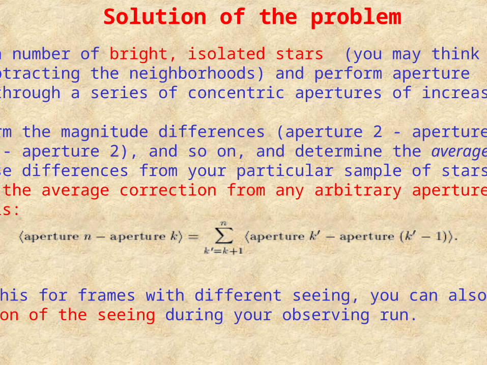
You choose a number of bright, isolated stars (you may think to createthem, by subtracting the neighborhoods) and perform aperture photometry through a series of concentric apertures of increasing radius.

Then you form the magnitude differences (aperture 2 - aperture 1), (aperture 3 - aperture 2), and so on, and determine the average value for each of these differences from your particular sample of stars in the frame. Then the average correction from any arbitrary aperture k to aperture n is:

If you do this for frames with different seeing, you can also account forthe variation of the seeing during your observing run.

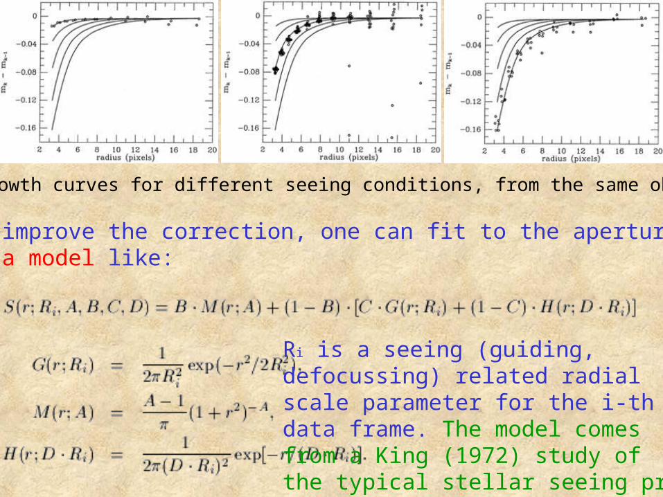
Examples of growth curves for different seeing conditions, from the same observing run.

In order to improve the correction, one can fit to the aperture photometrydifferences a model like:

Ri is a seeing (guiding, defocussing) related radial scale parameter for the i-thdata frame. The model comesfrom a King (1972) study ofthe typical stellar seeing profile.

Non-standard photometric systems

What shall we do in case we do not have a standard photometric system,with an appropriate set of standard stars?It must be clearly stated that when the transmission curves of the equipment used to collect the observations are rather different from those of any existing standard system, the transformation of the data to a standard system can be totally unreliable, particularly for extremestars (i.e., extreme colors, unusual spectral type, high reddening, etc.).

If we are dealing with groundbased obsevations…it is a long, tedious,delicate job, and I do not have the time to enter into the problem here.Do you want an advice? Change telescope!

Unfortunatlely, also widely desired (!) and widely used telescopes likeHST….have imagers which do not mount “standard” filters.Do you want an advice? Do not attempt to transform your WFPC2 orACS instrumental magnitudes into any standard system!

So, what shall we do?

Provided that the transmission curves of the complete optical system and detectors are known, a calibration of the zero points into physical units is easy to obtain by using a reference star for which the spectral flux (outside the atmosphere) as a function of the wavelength is known (e.g. Vega). By multiplying the reference spectrum by the system transmission curves one obtains the flux within the given pass bands, which can be easily transformed into magnitudes. If one uses the same procedure employing model atmospheres and theoretical fluxes, it is possible to relate the magnitudes and colors to the physical parameters like temperature and luminosity.

I think that Bedin et al. (2004) have written a paper which describes in a complete and clear way the methodology, applying it to the calibration of the HST/ACS camera.A similar method has been applied by Holtzman et al. (1995) andDolphin (2000) for the calibration of the HST/WFPC2 camera.

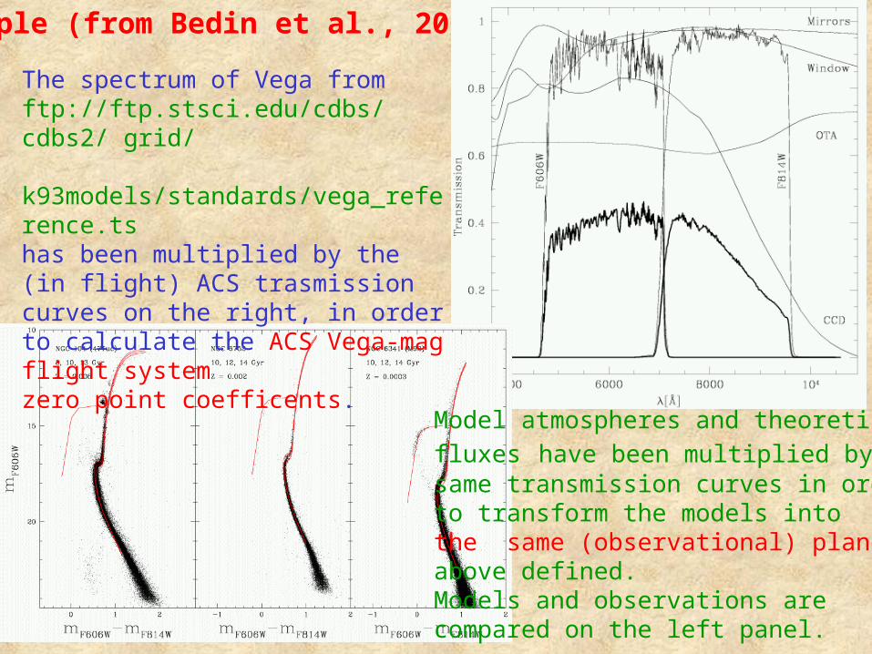
Example (from Bedin et al., 2004):

The spectrum of Vega fromftp://ftp.stsci.edu/cdbs/cdbs2/ grid/ k93models/standards/vega_reference.tshas been multiplied by the (in flight) ACS trasmission curves on the right, in order to calculate the ACS Vega-mag flight system zero point coefficents.

Model atmospheres and theoretical

fluxes have been multiplied by the same transmission curves in order to transform the models into the same (observational) plane above defined.Models and observations are compared on the left panel.