Embed Size (px)
Citation preview

Good and Bad Uncertainty:Macroeconomic and Financial Market ImplicationsI
Gill Segala, Ivan Shaliastovicha,∗, Amir Yarona,1
aThe Wharton School, University of Pennsylvania, 3620 Locust Walk, Philadelphia, PA 19104, USA
Abstract
Does macroeconomic uncertainty increase or decrease aggregate growth and asset prices? To address this question, we de-compose aggregate uncertainty into ‘good’ and ‘bad’ volatility components, associated with positive and negative innovations tomacroeconomic growth. We document that in line with our theoretical framework, these two uncertainties have opposite impacton aggregate growth and asset prices. Good uncertainty predicts an increase in future economic activity, such as consumption,output, and investment, and is positively related to valuation ratios, while bad uncertainty forecasts a decline in economic growthand depresses asset prices. Further, the market price of risk and equity beta of good uncertainty are positive, while negative forbad uncertainty. Hence, both uncertainty risks contribute positively to risk premia, and help explain the cross-section of expectedreturns beyond cash flow risk.
Keywords: Uncertainty, economic growth, asset prices, recursive utilityJEL: G12, E20, C58
IWe thank the Journal Editor, an anonymous referee, and participants and the discussants at 2014 AEA Meeting, 7th Annual SoFiE Conference,2014 Brazilian Finance Society Meeting, 2014 CIREQ Montreal Econometrics Conference, 2013 Minnesota Macro-Asset Pricing Conference,2014 SED Meeting, 2014 NBER Summer Institute, 2014 NBER’s Universities Research Conference, 2014 Tel Aviv Finance Conference, 2013Tepper-LAEF Conference, 2014 UBC Winter Finance Conference, 2014 WFA Meeting, University of Chicago Conference Honoring Lars Hansen,BI Norwegian Business School, Boston College, CKGSB, Federal Reserve Board, IDC, LBS, LSE, OSU, Princeton, SAIF-Tsinghua, Universityof Frankfurt, University of Miami, University of Notre-Dame, and Wharton for their comments and suggestions. Shaliastovich and Yaron thankJacobs Levy Equity Management Center for Quantitative Financial Research and the Rodney White Center, and Shaliastovich thanks the Cynthiaand Bennett Golub Endowment for financial support.∗Corresponding author. Tel: + 1 215 746 0005.Email addresses: [email protected] (Gill Segal), [email protected] (Ivan Shaliastovich),
[email protected] (Amir Yaron)1Amir Yaron is also a Research Associate at the NBER.
1

1. Introduction
How do changes in economic uncertainty affect macroeconomic quantities and asset prices? We show that the
answer to this question hinges on the type of uncertainty one considers. ’Bad’ uncertainty is the volatility that is
associated with negative innovations to macroeconomic quantities (e.g., output, consumption, earnings), and with
lower prices and investment, while ’good’ uncertainty is the volatility that is associated with positive shocks to these
variables, and with higher asset prices and investment.
To illustrate these two types of uncertainties, it is instructive to consider two episodes: (i) the high-tech revolution
of early-mid 1990’s, and (ii) the recent collapse of Lehman brothers in the fall of 2008. In the first case, and with the
introduction of the world-wide-web, a common view was that this technology would provide many positive growth
opportunities that would enhance the economy, yet it was unknown by how much? We refer to such a situation as
‘good’ uncertainty. Alternatively, the second case marked the beginning of the global financial crisis, and with many
of the ensuing bankruptcy cases one knew that the state of economy was deteriorating - yet, again, it was not clear by
how much? We consider this situation as a rise in ‘bad’ uncertainty. In both cases, uncertainty level rises relative to
its long-run steady-state level, yet, the first case coincides with an optimistic view, and the second with a pessimistic
one.
In this paper, we demonstrate that variations in good and bad uncertainty have separate and significant opposing
impacts on the real economy and asset prices. We use an extended version of the long-run risks model of Bansal
and Yaron (2004) to theoretically show conditions under which good and bad uncertainty have different impact on
prices. To make a meaningful distinction between good and bad uncertainty, we decompose, within the model,
the overall shocks to consumption into two separate zero-mean components (e.g., jumps) which capture positive
and negative growth innovations. The volatilities of these two shocks are time varying, and capture uncertainty
fluctuations associated with the positive and negative parts of the distribution of consumption growth. Thus, in the
model, valuation ratios are driven by three state variables: predictable consumption growth, good uncertainty, and bad
uncertainty. Consequently, the stochastic discount factor, and therefore risk premia, are determined by three sources
of risk: cash flow, good uncertainty, and bad uncertainty risks.
We show that with a preference for early resolution of uncertainty, the direct impact of both types of uncertainty
shocks is to reduce prices, though, prices respond more to bad than to good uncertainty. For prices to rise in response
to a good uncertainty shock there has to be an explicit positive link between good uncertainty and future growth
prospects – a feature that we impose in our benchmark model.2 We further show that the market price of good
uncertainty risk and its equity beta have the same (positive) sign. Thus, even though prices can rise in response to
good uncertainty, it commands a positive risk premium.
Overall the model’s key empirical implications include: (i) good uncertainty positively predicts future measures
2Backus et al. (2010) also feature a direct feedback from volatility to future growth. However, they focus on total volatility and show theimportance of this feedback for reconciling various lead-lag correlations between consumption growth and market returns.
2

of economic activity, while bad uncertainty negatively forecasts future economic growth; (ii) good uncertainty fluc-
tuations are positively related to asset valuations and to the real risk-free rate, while an increase in bad uncertainty
depresses asset prices and the riskless yield; and (iii) the shocks to good and bad uncertainty carry positive and
negative market prices of risk, respectively, yet both contribute positively to the risk premium.3
We evaluate our model’s empirical implications by utilizing a novel econometric approach to identify good and
bad uncertainty from higher-frequency realized variation in the variables of interest (see Barndorff-Nielsen et al.
(2010)). Empirically, we use the ex-ante predictable components of the positive and negative realized semivariances
of industrial production growth rate as the respective proxies for good and bad uncertainty.4 In its limiting behavior,
positive (negative) semivariance captures one-half of the variation in any Gaussian symmetric movements in the
growth rate of the variable of interest, as well as the variation of any non-Gaussian positive (negative) component in
it. Thus, in our empirical work the positive (negative) semivariance captures the volatility component that is associated
with the positive (negative) part of the total variation of industrial production growth, and its predictive component
corresponds to the model concept for good (bad) uncertainty.
Consistent with the model, we document in the data that across various macroeconomic growth rates, and across
various horizons, good economic uncertainty positively predicts future growth. This evidence includes growth for
horizons of one to five years in consumption, output, investment, R&D, market earnings, and dividends. Similarly, we
find a negative relationship between bad uncertainty and future growth rates of these macro variables. Together, these
findings support the model feedback channel from macroeconomic uncertainty to future growth rates. Quantitatively,
the impact of uncertainty has a large economic effect on the macro variables. For example, the private GDP growth
increases by about 2.5% one year after a one standard deviation shock to good uncertainty, and this positive effect
persists over the next three years. On the other hand, bad uncertainty shocks decrease output growth by about 1.3%
one year after and their effects remain negative for several years. The responses of investment and R&D to these
shocks are even stronger. Both capital and R&D investment significantly increase with good uncertainty and remain
positive five years out, while they significantly drop with a shock to bad uncertainty. An implication of the offsetting
responses to good and bad uncertainty is that the measured responses to overall uncertainty are going to be muted.
Indeed, GDP growth declines only by about 0.25% after a shock to total uncertainty. The response to total uncertainty
is significantly weaker than that to bad uncertainty, which underscores the potential importance of decomposing
uncertainty into good and bad components.
The empirical evidence in the data is further consistent with the model’s key asset-pricing implications. We
document that the market price-dividend ratio and the risk-free rate appreciate with good uncertainty and decline
with bad uncertainty. Quantitatively, the market log price-dividend ratio rises by about 0.07 one year out in response
to a one standard deviation shock to good uncertainty and remains positive ten years afterward. Bad uncertainty
3Although both uncertainties carry positive risk premium, their covariance, which may capture a common component, could contribute nega-tively to the risk premium.
4We use industrial production because high-frequency real consumption data is not available for the long sample.
3

shock depresses the log price-dividend ratio by 0.06 on impact and remains negative for ten years out. Similar to the
macroeconomic growth rates, the response of the price-dividend ratio to total uncertainty is negative, but is understated
relative to the response to bad uncertainty. The evidence for the response of the price-earnings ratio is very similar to
that of the price-dividend ratio. In addition, consistent with the model, we show that both bad and good uncertainty
positively predict future excess returns and their volatility.
Finally, we estimate the market prices of good and bad volatility risks using the cross-section of asset returns
that includes the market return, 25 equity portfolios sorted on book-to-market ratio and size, and two bond portfolios
(Credit and Term Premium portfolios). We show that the market price of risk is positive for good uncertainty, while
it is negative for bad uncertainty. Moreover, asset returns have a positive exposure (beta) to good uncertainty risk,
and a negative exposure to bad uncertainty risk. Consequently, both good and bad uncertainty command a positive
risk premium, although the interaction of their shocks can contribute negatively to the total risk compensation, since
the good and bad uncertainty shocks are positively correlated. The market risk premium is 7.2% in the data relative
to 8.2% in the model. In the data, the value spread is 4.38%, which is comparable to 3.34% in the model. The size
spread is 4.39%, relative to 5.21% in the model. For the Credit premium portfolio the risk premium is 1.98% in the
data and 2.15% in the model, and the Term premium is 1.82% in the data relative to 0.64% in the model.
Related Literature. Our paper is related to a growing theoretical and empirical literature that documents the con-
nection between economic uncertainty, aggregate quantities, and asset prices. Our concept of economic uncertainty
refers to the time series volatility of shocks to economic quantity variables of interest (e.g., consumption and GDP
growth). This is distinct from other aspects of uncertainty, such as parameter uncertainty, learning, robust-control, and
ambiguity (see discussions in Pastor and Veronesi (2009), Hansen and Sargent (2010), Epstein and Schneider (2010)).
While there is a long standing and voluminous literature on the time-varying second moments in asset returns, the
evidence for time variation in the second moments of macro aggregates, such as consumption, dividends, earnings,
investment, and output, is more limited and recent. Kandel and Stambaugh (1991) is an early paper providing ev-
idence for stochastic volatility in consumption growth. More recently, McConnell and Perez-Quiros (2000), Stock
and Watson (2002), and Bansal et al. (2005b) provide supporting evidence that volatility measures based on macro
aggregates feature persistent predictable variation.
The evidence on time-varying volatility of macro aggregates has also instilled recent interest in examining the role
of uncertainty in production/DSGE models. Bloom (2009) shows that increased volatility, measured via VIX, leads
to an immediate drop in consumption and output growth rates as firms delay their investment decisions. Generally the
literature has emphasized a negative relationship between growth and uncertainty – see Ramey and Ramey (1995),
Gilchrist et al. (2010), Fernandez-Villaverde et al. (2011), and Basu and Bundick (2012) to name a few. Other
papers, such as Gilchrist and Williams (2005), Jones et al. (2005), Malkhozov and Shamloo (2010), and Kung and
Schmid (2010) feature alternative economic channels which can generate positive relationship between uncertainty
and investment and thus growth. In addition, Croce et al. (2012) and Pastor and Veronesi (2012) highlight the negative
impact of government policy uncertainty on prices and growth.4

In terms of asset prices, Bansal and Yaron (2004) show that with Epstein and Zin (1989) recursive preferences
and an IES larger than one, economic uncertainty is a priced risk, and is negatively related to price-dividend ratios.
More recently, Bansal et al. (2013) examine the implications of macroeconomic volatility for the time variation in
risk premia, for the return on human capital, and for the cross-section of returns. They develop a dynamic CAPM
framework for which one of the factors, in addition to the standard cash flow and discount rate risks, is aggregate
volatility. Campbell et al. (2012) also analyze the role of uncertainty in an extended version of the ICAPM. While
both papers document a significant role for uncertainty, Bansal et al. (2013) find both the betas and market price
of uncertainty risk to be negative, and thus uncertainty to positively contribute to equity risk premia, whereas the
evidence in Campbell et al. (2012) is more mixed in terms of whether assets have negative or positive exposure
(beta) to volatility. The empirical framework in this paper, allowing for two types of uncertainties, can in principle
accommodate several of these uncertainty effects.
Our framework features two types of macroeconomic uncertainties. In terms of estimating two types of uncertain-
ties, the literature has mainly focused on return-based measures. Patton and Sheppard (2011), Feunou et al. (2013),
and Bekaert et al. (2014) use return data to capture fluctuations in good and bad volatilities, and study their effects on
the dynamics of equity returns. Specifically, Patton and Sheppard (2011) and Feunou et al. (2013) use realized semi-
variance measures to construct the two volatilities, whereas we construct bad and good uncertainty measures directly
from the macro aggregates.
Our framework is also related to a recent literature which highlights non-Gaussian shocks in the fundamentals.
One analytically convenient specification that our framework accommodates and which is widely used features Pois-
son jumps in consumption dynamics (see e.g. Eraker and Shaliastovich (2008), Benzoni et al. (2011), Drechsler and
Yaron (2011), and Tsai and Wachter (2014) for recent examples). In another specification, which again can be ac-
commodated within our framework, the cash flow shocks are drawn from a Gamma distribution with a time-varying
shape parameter, in which case the consumption shock dynamics follow the good and bad environment specification in
Bekaert and Engstrom (2009). Finally, an alternative approach for generating time variation in higher-order moments
is provided in Colacito et al. (2013). They model shocks to expected consumption as drawn from a skew-normal distri-
bution with time-varying parameters and allow for a separate process for stochastic volatility. Our modeling approach
focuses on bad and good volatility as the key driving forces for time variation in consumption growth distribution, and
is largely motivated by our empirical analysis.
There is also a voluminous literature on the implications of time-varying higher-order moments of returns for risk
pricing. For example, Bansal and Viswanathan (1993) develops a nonlinear pricing kernel framework and shows its
improvement in explaining asset prices relative to a linear APT model, while Chabi-Yo (2012) develops an intertem-
poral capital asset pricing model in which innovations in higher moments are priced. The empirical literature identifies
these risks based on financial market data, and generally finds that left-tail risk is important for explaining the time
series and cross-section of returns above and beyond the market volatility risk; see e.g. Kapadia (2006), Adrian and
5

Rosenberg (2008), Harvey and Siddique (2000), Chang et al. (2013), and Conrad et al. (2013).5
The rest of this paper is organized as follows. In Section 2 we provide a theoretical framework for good and bad
uncertainty and highlight their role for future growth and asset prices. Section 3 discusses our empirical approach to
construct good and bad uncertainty in the macroeconomic data. In Section 4 we show our empirical results for the
effect of good bad uncertainties on aggregate macro quantities and aggregate asset prices, and the role of uncertainty
risks for the market return and the cross-section of risk premia. Section 5 discusses the robustness of our key empirical
results, and the last Section provides concluding comments.
2. Economic Model
To provide an economic structure for our empirical analysis, in this section we lay out a version of the long-run
risks model that incorporates fluctuations in good and bad macroeconomic uncertainties. We use our economic model
to highlight the roles of the good and bad uncertainties for future growth and the equilibrium asset prices.
2.1. Preferences
We consider a discrete-time endowment economy. The preferences of the representative agent over the future
consumption stream are characterized by the Kreps and Porteus (1978) recursive utility of Epstein and Zin (1989) and
Weil (1989):
Ut =
[(1 − β)C
1−γθ
t + β(EtU1−γt+1 )
1θ
] θ1−γ
, (1)
where Ct is consumption, β is the subjective discount factor, γ is the risk-aversion coefficient, and ψ is the elasticity
of intertemporal substitution (IES). For ease of notation, the parameter θ is defined as θ ≡ 1−γ1− 1
ψ
. Note that when θ = 1,
that is, γ = 1/ψ, the recursive preferences collapse to the standard case of expected power utility, in which case the
agent is indifferent to the timing of the resolution of uncertainty of the consumption path. When risk aversion exceeds
the reciprocal of IES (γ > 1/ψ), the agent prefers early resolution of uncertainty of consumption path, otherwise, the
agent has a preference for late resolution of uncertainty.
As is shown in Epstein and Zin (1989), the logarithm of the intertemporal marginal rate of substitution implied by
these preferences is given by:
mt+1 = θlog β −θ
ψ∆ct+1 + (θ − 1)rc,t+1, (2)
where ∆ct+1 = log(Ct+1/Ct) is the log growth rate of aggregate consumption, and rc,t is a log return on the asset
which delivers aggregate consumption as dividends (the wealth portfolio). This return is different from the observed
return on the market portfolio as the levels of market dividends and consumption are not the same. We solve for the
5See also a related literature on market downside risk, e.g., Ang et al. (2006) and Lettau et al. (2014), which emphasizes the importance ofmarket left-tail risk.
6

endogenous wealth return and the equilibrium stochastic discount factor in (2) using the dynamics for the endowment
process and the standard Euler equation,
Et[expmt+1Ri,t+1
]= 1, (3)
which hold for the return on any asset in the economy, Ri,t+1, including the wealth portfolio.
2.2. Consumption Dynamics
Our specification of the endowment dynamics incorporates the underlying channels of the long-run risks model
of Bansal and Yaron (2004), such as the persistent fluctuations in expected growth and the volatility of consumption
process. The novel ingredients of our model include: (i) the decomposition of the total macroeconomic volatility into
good and bad components associated with good and bad consumption shocks, respectively, and (ii) the direct effect
of macroeconomic volatilities on future economic growth. We show that these new model features are well-motivated
empirically and help us interpret the relation between the good and bad uncertainties, the economic growth, and the
asset prices in the data.
Our benchmark specification for the consumption dynamics is written as follows:
∆ct+1 = µc + xt + σc(εg,t+1 − εb,t+1), (4)
xt+1 = ρxt + τgVgt − τbVbt
+σx(εg,t+1 − εb,t+1), (5)
where xt is the predictable component of next-period consumption growth, and εgt+1 and εbt+1 are two mean-zero
consumption shocks which for parsimony affect both the realized and expected consumption growth.6 The shocks εgt+1
and εbt+1 separately capture positive and negative shocks in consumption dynamics, respectively, and are modelled as,
εi,t+1 = εi,t+1 − Etεi,t+1, for i = g, b, (6)
where the underlying shocks εi,t+1 have a positive support, namely, εi,t+1 > 0 for i = g, b. This ensures that the
consumption shocks εgt+1 and εbt+1 are conditionally mean zero, and are driven by positive and negative shocks to
consumption growth, respectively.
We assume that the volatilities of consumption shocks are time varying and driven by the state variables Vgt and
Vbt; in particular,
Vartεg,t+1 = Vartεg,t+1 ≡ Vgt,
Vartεb,t+1 = Vartεb,t+1 ≡ Vbt.
6It is straightforward to extend the specification to allow for separate shocks in realized and expected consumption growth rates and break theperfect correlation of the two. This does not affect our key results, and so we do not entertain this case to ease the exposition.
7

This allows us to interpret Vgt and Vbt as good and bad macroeconomic uncertainties, that is, uncertainties regarding
the right and left tail movements in consumption growth. In our specification, the good and bad uncertainties follow
separate AR(1) processes,
Vg,t+1 = (1 − νg)Vg0 + νgVgt + σgwwg,t+1, (7)
Vb,t+1 = (1 − νb)Vb0 + νbVbt + σbwwb,t+1, (8)
where for i = g, b, Vi0 is the level, νi the persistence, and wi,t+1 the shock in the uncertainty. For simplicity, the
volatility shocks are Normally distributed, and we let α denote the correlation between the good and bad volatility
shocks.
By construction, the macro volatilities govern the magnitude of the good and bad consumption innovation. In
addition to that, our feedback specification in (5) also allows for a direct effect of good and bad macro uncertainty
on future levels of economic growth. Backus et al. (2010) use a similar feedback specification from a single (total)
volatility to future growth. Our specification features two volatilities (good and bad), and for τg > 0 and τb > 0, an
increase in good volatility raises future consumption growth rates, while an increase in bad volatility dampens future
economic growth. The two-volatility specification captures, in a reduced-form way, an economic intuition that good
uncertainty, through the positive impact of new innovation on growth opportunities, would increase investment and
hence future economic growth, while bad uncertainty, due to the unknown magnitude of adverse news and its impact
on investment, would result in lower growth in the future. While we do not provide the primitive micro-foundation for
this channel, we show direct empirical evidence to support our volatility feedback specification. Further, we show that
the volatility feedback for future cash flows also leads to testable implications for the asset prices which are supported
in the data.
It is important to note that our specification for consumption growth displays non-Gaussian dynamics with time-
varying mean, volatility, and higher-order moments. Specifically, total consumption volatility is equal to the sum of
the good and bad uncertainties, Vgt +Vbt, whereas skewness, kurtosis, and all other higher moments are functions of the
underlying volatility variables Vgt and Vbt. The specific way in which Vgt and Vbt affect those higher moments depends
on the underlying distribution for εi,t+1, i = b, g. One specification that is analytically convenient and widely used
features Poisson jumps in the consumption fundamentals, in which case, skewness is directly related to fluctuations in
the intensity of jumps. In this case, the time variation in jump intensity affects separately the left and right tails of the
consumption distribution, and hence the movements in good and bad volatility and higher-order moments. Another
specification is one in which εi,t+1 are drawn from a Gamma distribution with a scale parameter 1 and a time-varying
shape parameter, in which case the consumption shocks dynamics follow the good and bad environment specification
in Bekaert and Engstrom (2009). The time-varying shape parameters governing the Gamma distribution drive the
variance and higher-order moments of consumption growth distribution. An alternative approach for generating time
variation in higher-order moments is given in Colacito et al. (2013). They model shocks to expected consumption as8

drawn from a skew-normal distribution with time-varying parameters and a separate process for stochastic volatility
which leads to separate movements in consumption volatility and skewness. Our modeling approach focuses on bad
and good volatility as the key driving forces for time variation in consumption growth distribution, which is largely
motivated by our empirical analysis.
2.3. Equilibrium Asset Prices
To get closed-form expressions for the equilibrium asset prices, we consider the consumption shock distribution
for which the log moment-generating function is linear in the underlying variances Vg,t and Vb,t. That is,
log Eteuεi,t+1 = f (u)Vi,t, for i = g, b, (9)
and the function f (u) captures the shape of the moment-generating function of the underlying consumption shocks. As
discussed earlier, prominent examples of such distributions include compound Poisson jump distribution and Gamma
distribution. As shown in Appendix Appendix B, for this class of distributions the function f (.) is non-negative,
convex, and asymmetric, that is, f (u) > f (−u) for u > 0.
We use a standard log-linearization approach to obtain analytical solutions to our equilibrium model. Below we
show a summary of our key results, and all the additional details are provided in Appendix Appendix B.
In equilibrium, the solution to the log price-consumption ratio on the wealth portfolio is linear in the expected
growth and the good and bad uncertainty states:
pct = A0 + Axxt + AgvVgt + AbvVbt. (10)
The slope coefficients are given by:
Ax =1 − 1
ψ
1 − κ1ρ,
Agv = Agv + τgκ1Ax
1 − κ1νg, Agv =
f (θ((1 − 1ψ
)σc + κ1Axσx))
θ(1 − κ1νg),
Abv = Abv − τbκ1Ax
1 − κ1νb, Abv =
f (−θ((1 − 1ψ
)σc + κ1Axσx))
θ(1 − κ1νg),
(11)
where the parameter κ1 ∈ (0, 1) is the log-linearization coefficient, and the As are the uncertainty loadings on the
price consumption ratio that would be obtained if the consumption dynamics did not include a direct feedback from
uncertainty to growth prospects, namely if τb = τg = 0.
As can be seen from the above equations, the response of the asset valuations to the underlying macroeconomic
states is pinned down by the preference parameters and model parameters which govern the consumption dynamics.
The solution to the expected growth loading Ax is identical to Bansal and Yaron (2004), and implies that when the
9

substitution effect dominates the wealth effect (ψ > 1), asset prices rise with positive growth prospects: Ax > 0.
The expressions for the uncertainty loadings are more general than the ones in the literature and take into account
our assumptions on the volatility dynamics. First, our specification separates positive and negative consumption
innovations which have their own good and bad volatility, respectively. The impact of this pure volatility channel
on asset prices is captured by the first components of the volatility loadings in (11), Agv and Abv. In particular, when
both γ and ψ are above one, these two loadings are negative: Agv, Abv < 0. That is, with a strong preference for early
resolution of uncertainty, the agent dislikes volatility, good or bad, so the direct effect of an increase in uncertainty
about either positive or negative tail of consumption dynamics is to decrease equilibrium equity prices. In the absence
of cash flow effect, both good and bad uncertainties depress asset valuations, albeit by a different amount. Indeed,
due to a positive skewness of underlying consumption shocks, an increase in good (bad) uncertainty asymmetrically
raises the right (left) tail of the future consumption growth distribution, and this asymmetry leads to a quantitatively
larger negative response of the asset prices to bad uncertainty than to good uncertainty: |Abv| > |Agv|.
In addition to the direct volatility effect, in our model the good and bad uncertainties can also impact asset prices
through their feedback on future cash flows (see equation 5). For τb > 0, the negative effect of bad uncertainty
on future expected growth further dampens asset valuations, and as shown in (11), the bad volatility coefficient Abv
becomes even more negative. On the other hand, when good uncertainty has a positive and large impact on future
growth, the cash flow effect of the good uncertainty can exceed its direct volatility effect, and as a result the total asset-
price response to good uncertainty becomes positive: Agv > 0. Hence, in our framework, good and bad uncertainties
can have opposite impact on equity prices, with bad uncertainty shocks decreasing and good uncertainty shocks
increasing asset valuations, which we show is an important aspect of the economic data.7
The aforementioned effect of uncertainty on asset valuations is related to several recent studies. In the context
of long-run risks models with preferences for early resolution of uncertainty, Eraker and Shaliastovich (2008) and
Drechsler and Yaron (2011) entertain jumps in cash flows and show that asset valuation drop with increase in jump
intensity, and in particular are sensitive to jumps which affect the left tail of consumption distribution. This effect on
prices is also reflected in Colacito et al. (2013) who show that asset valuations decline when skewness becomes more
negative. Tsai and Wachter (2014) consider a specification that incorporate time-varying rare disasters and booms. As
their Poisson jump shocks are uncompensated, the intensities of booms and disasters have a direct impact on expected
growth and thus capture the differential τ effects highlighted above, which leads to a differential impact of jump
intensity on prices. Finally, in the context of the habits model in Bekaert and Engstrom (2009) prices decline at times
of high expected growth and increase at times of good or bad variance of Gamma-distributed consumption growth
shocks. The difference in the response of prices to uncertainty relative to our specification is due to the preference
structure, and in particular, the preference for early resolution of uncertainty.
7Note that in our simple endowment economy, welfare is increasing in the value of the consumption claim. When Agv is positive, the implicationis that good uncertainty shock increases welfare. This is not surprising since for Agv to be positive there must be a significant positive feedbackfrom this uncertainty to future growth. The bad uncertainty, as in Bansal and Yaron (2004), unambiguously reduces welfare.
10

In the model, the good and bad uncertainty can also have different implications on equilibrium risk-free rates.
Using a standard Euler equation (3), the solutions to equilibrium yields on n−period real bonds are linear in the
underlying state variables:
yt,n =1n
(B0,n + Bx,nxt + Bgv,nVgt + Bbv,nVbt), (12)
where Bx,n, Bgv,n and Bbv,n are the bond loadings to expected growth, good, and bad uncertainty factors, whose solu-
tions are provided in the Appendix. As shown in the literature, real bond yields increase at times of high expected
growth, and the bond loading Bx,n is positive. Further, an increase in either good and bad uncertainty raises the pre-
cautionary savings motive for the representative agent, so the direct impact of either uncertainty on risk-free rates is
negative. However, in addition to the direct volatility effect, in our framework good and bad uncertainties also have
an impact on future economic growth. Similar to the discussion of the consumption claim, bad uncertainty reduces
future growth rates which further dampens real rates, so Bbv,n becomes more negative. On the other hand, the positive
cash flow impact of good volatility can offset the precautionary savings motive at longer maturities and can lead to a
positive response of interest rates to good uncertainty. Thus, due to the volatility feedback, in our framework good
and bad uncertainties can have opposite effect on the risk-free rates, which we show is consistent with the data.
2.4. Risk Compensation
Using the model solution to the price-consumption ratio in (10), we can provide the equilibrium solution to the
stochastic discount factor in terms of the fundamental states and the model and preference parameters. The innovation
in the stochastic discount factor, which characterizes the sources and magnitudes of the underlying risk in the economy,
is given by:
mt+1 − Et[mt+1] = −λxσx(εg,t+1 − εb,t+1)
−λgvσgwwg,t+1
−λbvσbwwb,t+1, (13)
and λx, λgv and λbv are the market-prices of risk of growth, good volatility, and bad volatility risks. Their solutions are
given by:
λx = (1 − θ)κ1Ax + γσc
σx(14)
λgv = (1 − θ)κ1Agv, (15)
λbv = (1 − θ)κ1Abv. (16)
When the agent has a preference for early resolution of uncertainty, the market price of consumption growth
risk λx is positive: λx > 0. Consistent with our discussion of the price-consumption coefficients, the market prices
11
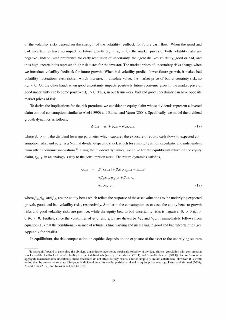
of the volatility risks depend on the strength of the volatility feedback for future cash flow. When the good and
bad uncertainties have no impact on future growth (τg = τb = 0), the market prices of both volatility risks are
negative. Indeed, with preference for early resolution of uncertainty, the agent dislikes volatility, good or bad, and
thus high uncertainties represent high risk states for the investor. The market prices of uncertainty risks change when
we introduce volatility feedback for future growth. When bad volatility predicts lower future growth, it makes bad
volatility fluctuations even riskier, which increase, in absolute value, the market price of bad uncertainty risk, so
λbv < 0. On the other hand, when good uncertainty impacts positively future economic growth, the market price of
good uncertainty can become positive: λgv > 0. Thus, in our framework, bad and good uncertainty can have opposite
market prices of risk.
To derive the implications for the risk premium, we consider an equity claim whose dividends represent a levered
claim on total consumption, similar to Abel (1990) and Bansal and Yaron (2004). Specifically, we model the dividend
growth dynamics as follows,
∆dt+1 = µd + φxxt + σdud,t+1, (17)
where φx > 0 is the dividend leverage parameter which captures the exposure of equity cash flows to expected con-
sumption risks, and ud,t+1 is a Normal dividend-specific shock which for simplicity is homoscedastic and independent
from other economic innovations.8 Using the dividend dynamics, we solve for the equilibrium return on the equity
claim, rd,t+1, in an analogous way to the consumption asset. The return dynamics satisfies,
rd,t+1 = Et[rd,t+1] + βxσx(εg,t+1 − εb,t+1)
+βgvσgwwg,t+1 + βbvσbw
+σdud,t+1, (18)
where βx, βgv, and βbv are the equity betas which reflect the response of the asset valuations to the underlying expected
growth, good, and bad volatility risks, respectively. Similar to the consumption asset case, the equity betas to growth
risks and good volatility risks are positive, while the equity beta to bad uncertainty risks is negative: βx > 0, βgv >
0, βbv < 0. Further, since the volatilities of εb,t+1 and εg,t+1 are driven by Vb,t and Vg,t, it immediately follows from
equation (18) that the conditional variance of returns is time varying and increasing in good and bad uncertainties (see
Appendix for details).
In equilibrium, the risk compensation on equities depends on the exposure of the asset to the underlying sources
8It is straightforward to generalize the dividend dynamics to incorporate stochastic volatility of dividend shocks, correlation with consumptionshocks, and the feedback effect of volatility to expected dividends (see e.g., Bansal et al. (2011), and Schorfheide et al. (2013)). As our focus is onaggregate macroeconomic uncertainty, these extensions do not affect our key results, and for simplicity are not entertained. However, it is worthnoting that, by convexity, separate idiosyncratic dividend volatility can be positively related to equity prices (see e.g., Pastor and Veronesi (2006),Ai and Kiku (2012), and Johnson and Lee (2013)).
12

of risk, the market prices of risks, and the quantity of risk. Specifically, the equity risk premium is given by,
EtRd,t+1 − R f ,t ≈ log Ererd,t+1−r f ,t
=[f (−λxσx) − f ((βx − λx)σx) + f (βxσx)
]Vgt
+[f (λxσx) − f ((λx − βx)σx) + f (−βxσx)
]Vbt
+ βgvλgvσ2gw + βgvλbvσ
2bw
+ ασbwσgw(βgvλbv + βbvλgv).
(19)
In our model, all three sources of risks contribute to the risk premia, and the direct contribution of each risk to the
equity risk premium is positive. The first two components of the equity premium above capture the contribution of
the non-Gaussian growth risk, which is time varying and driven by the good and bad volatilities. When γ > 1 and
ψ > 1, the market price of growth risk λx and the equity exposure to growth risk βx are both positive. As we show in
the Appendix, this implies that the equity premium loadings on both good and bad volatilities are positive, so that the
growth risks receive positive risk compensation unconditionally, and this risk compensation increases at times of high
good or bad volatility. The remaining constant components in the equity risk premia equation capture the contributions
of the Gaussian volatility shocks. As the market prices of volatility risks and equity exposure to volatility risks have
the same sign, the volatility risks receive positive risk compensation in equities. The last term in the decomposition
above captures the covariance between good and bad uncertainty risk, and is negative when the two uncertainties have
positive correlation (α > 0).
To get further intuition for the nature of the risk compensation, we consider a Taylor expansion of the equity risk
premium:
EtRd,t+1 − R f ,t ≈ const + βxλxσ2x(Vgt + Vbt)
− λxβxσ3x(λx − βx)(Vgt − Vbt) + . . .
(20)
The constant in this equation captures constant contribution of volatility risks to the risk premia. Subsequent terms
pick out the second and third-order components in the decomposition of the non-Gaussian growth risk premia; for
simplicity, we omit higher-order terms. The second-order component is standard, and is equal to the negative of
the covariance of log returns and log stochastic discount factor. This component is driven by the quantity of total
consumption variance, Vgt +Vbt.An increase in either good or bad volatility directly raises total consumption variance,
and hence increases equity risk premia (βx and λx are both positive). The third-order component is driven by the
quantity of consumption skewness, Vgt − Vbt. Under typical parameter calibration of the model, λx > βx.9 This
9In the model, λx = (1 − θ)κ1Ax + γσc/σx, and βx = κ1,dHx. The term (1 − θ) is positive under early resolution of uncertainty, and amounts to28 under a typical calibration of γ = 10, ψ = 1.5. The equity price response to growth news Hx is magnified relative to consumption asset priceresponse Ax by the leverage of the dividend stream φx, so that Hx/Ax is around 3-5. The log-linearization parameters κ1 ≈ κ1,d ≈ 1. In all, thisprovides, λx > βx.
13

implies that when Vbt increases relative to Vgt and the skewness of consumption shocks decreases (becomes more
negative), the equity premium goes up. Hence, the total risk premium increases at times of high good or bad volatility,
but the bad volatility has a larger effect capturing the importance of the left tails.
The quantities of total consumption variance and skewness risk are time varying themselves, and directly con-
tribute to the equity risk premium. In our model, the total variance and skewness are linearly related to the good
and bad volatilities, so that the risk compensation for the variance and skewness risk are components of the constant
risk compensation for good and bad volatility risks in (19)-(20). We show the implied market prices and equity be-
tas to variance and skewness risk in the Appendix. In particular, in our framework agents dislike states with low
consumption growth skewness (larger left tails), thus leading asset prices to fall in those states.
3. Data and Uncertainty Measures
3.1. Data
In our benchmark analysis we use annual data from 1930 to 2012. Consumption and output data come from the
Bureau of Economic Analysis (BEA) NIPA tables. Consumption corresponds to the real per capita expenditures on
non-durable goods and services and output is real per capita gross domestic product minus government consumption.
Capital investment data are from the NIPA tables; R&D investment is available at the National Science Foundation
(NSF) for the 1953 to 2008 period, and the R&D stock data are taken from the BEA Research and Development
Satellite Account for the 1959 to 2007 period. To measure the fluctuations in macroeconomic volatility, we use
monthly data on industrial production from the Federal Reserve Bank of St. Louis.
Our aggregate asset-price data include 3-month Treasury bill rate, the stock price and dividend on the broad market
portfolio from CRSP, and aggregate earnings data from Shiller’s website. We adjust nominal short-term rate by the
expected inflation to obtain a proxy for the real risk-free rate. Additionally, we collect data on equity portfolios
sorted on key characteristics, such as book-to-market ratio and size, from the Fama-French Data Library. Our bond
portfolios, as in Ferson et al. (2013), include the excess returns of low- over high-grade corporate bonds (Credit
Premium portfolio), and the excess returns of long- over short-term Treasury bonds (Term premium portfolio).10.
To measure the default spread, we use the difference between the BAA and AAA corporate yields from the Federal
Reserve Bank of St. Louis.
The summary statistics for the key macroeconomic variables are shown in Panel A of Table 1. Over the 1930 to
2012 sample period the average consumption growth is 1.8% and its volatility is 2.2%. The average growth rates in
output, capital investment, market dividends, and earnings are similar to that in consumption, and it is larger for the
R&D investment (3.5%) over the 1954 to 2008 period. As shown in the Table, many of the macroeconomic variables
are quite volatile relative to consumption: the standard deviation of earnings growth is 26%, of capital investment
10We thank Wayne Ferson for providing us data on these bond portfolios which we extend till 2012 using long-term government data andcorporate bond data from Barclays.
14
growth is almost 15%, and of the market dividend growth is 11%. Most of the macroeconomic series are quite
persistent with an AR(1) coefficient of about 0.5.
Panel B of Table 1 shows the summary statistics for the key asset-price variables. The average real log market
return of 5.8% exceeds the average real rate of 0.3%, which implies an equity premium (in logs) of 5.5% over the
sample. The market return is also quite volatile relative to the risk-free rate, with a standard deviation of almost 20%
compared to 2.5% for the risk-free rate. The corporate yield on BAA firms is on average 1.2% above that for the AAA
firms, and the default spread fluctuates significantly over time. The default spread, real risk-free rate, and the market
price-dividend ratio are very persistent in the sample, and their AR(1) coefficients range from 0.72 to 0.88.
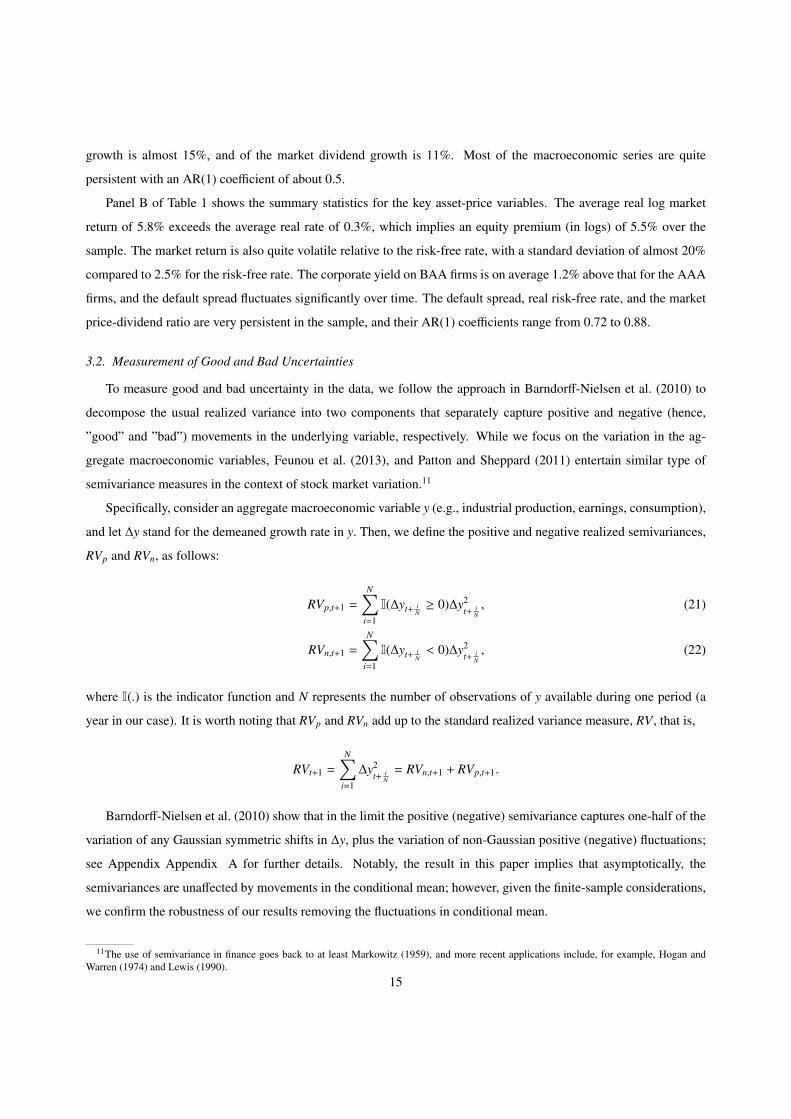
3.2. Measurement of Good and Bad Uncertainties
To measure good and bad uncertainty in the data, we follow the approach in Barndorff-Nielsen et al. (2010) to
decompose the usual realized variance into two components that separately capture positive and negative (hence,
”good” and ”bad”) movements in the underlying variable, respectively. While we focus on the variation in the ag-
gregate macroeconomic variables, Feunou et al. (2013), and Patton and Sheppard (2011) entertain similar type of
semivariance measures in the context of stock market variation.11
Specifically, consider an aggregate macroeconomic variable y (e.g., industrial production, earnings, consumption),
and let ∆y stand for the demeaned growth rate in y. Then, we define the positive and negative realized semivariances,
RVp and RVn, as follows:
RVp,t+1 =
N∑i=1
I(∆yt+ iN≥ 0)∆y2
t+ iN, (21)
RVn,t+1 =
N∑i=1
I(∆yt+ iN< 0)∆y2
t+ iN, (22)
where I(.) is the indicator function and N represents the number of observations of y available during one period (a
year in our case). It is worth noting that RVp and RVn add up to the standard realized variance measure, RV , that is,
RVt+1 =
N∑i=1
∆y2t+ i
N= RVn,t+1 + RVp,t+1.
Barndorff-Nielsen et al. (2010) show that in the limit the positive (negative) semivariance captures one-half of the
variation of any Gaussian symmetric shifts in ∆y, plus the variation of non-Gaussian positive (negative) fluctuations;
see Appendix Appendix A for further details. Notably, the result in this paper implies that asymptotically, the
semivariances are unaffected by movements in the conditional mean; however, given the finite-sample considerations,
we confirm the robustness of our results removing the fluctuations in conditional mean.
11The use of semivariance in finance goes back to at least Markowitz (1959), and more recent applications include, for example, Hogan andWarren (1974) and Lewis (1990).
15

The positive and negative semivariances are informative about the realized variation associated with movements in
the right and left tail, respectively, of the underlying variable. Positive (negative) semivariance therefore corresponds
to good (bad) realized variance states of the underlying variable and thus we use the predictable component of this
measure as the empirical proxy for ex-ante good (bad) uncertainty. To construct the predictive components, we project
the logarithm of the future average h−period realized semivariance on the set of time t predictors Xt :
log
1h
h∑i=1
RV j,t+i
= const j + ν′jXt + error, j = p, n, (23)
and take as the proxies for the ex-ante good and bad uncertainty Vg and Vb the exponentiated fitted values of the
projection above:
Vg,t = exp(constp + ν′pXt
), Vb,t = exp
(constn + ν′nXt
). (24)
The log transformation ensures that our ex-ante uncertainty measures remain strictly positive.
In addition to measuring the ex-ante uncertainties, we use a similar approach to construct a proxy for the expected
consumption growth rate, xt which corresponds to the fitted value of the projection of future consumption growth on
the same predictor vector Xt :
1h
h∑i=1
∆c j,t+i = constc + ν′cXt + error,
xt = constc + ν′cXt.
In our empirical applications we let y be industrial production, which is available at monthly frequency, and use
that to construct realized variance at the annual frequency. As there are twelve observations of industrial production
within a year, our measurement approach is consistent with the model setup which allows for multiple good and bad
shocks within a period (a year). To reduce measurement noise in constructing the uncertainties, in our benchmark
empirical implementation we set the forecast window h to three years. Finally, the set of the benchmark predictors
Xt includes positive and negative realized semivariances RVp,RVn, consumption growth ∆c, the real-market return rd,
the market price-dividend ratio pd, the real risk-free rate r f , and the default spread de f .12
Panel C of Table 1 reports the key summary statistics for our realized variance measures. The positive and negative
semivariances contribute about equally to the level of the total variation in the economic series, and the positive
semivariance is more volatile than the negative one. The realized variation measures co-move strongly together: the
contemporaneous correlation between total and negative realized variances is 80%, and the correlation between the
positive and negative realized variance measures is economically significant, and amounts to 40%.
12As shown in Section 5, our results are robust to using standard OLS regression instead of the log, the use of alternative predictors, differentforecast windows h, removing the conditional mean in constructing the semivariance measures, and using other measures for y.
16

Figure 1 shows the plot of the total realized variance, smoothed over the 3-year window to reduce measurement
noise. As can be seen from the graph, the overall macroeconomic volatility gradually declines over time, consistent
with the evidence in McConnell and Perez-Quiros (2000) and Stock and Watson (2002), as well as Bansal et al.
(2005b), Lettau et al. (2008), and Bansal et al. (2013). Further, the realized variance is strongly counter-cyclical:
indeed, its average value in recessions is twice as large as in expansions. The most prominent increases in the realized
variance occur in the recessions of the early and late 1930s, the recession in 1945, and more recently in the Great
Recession in the late 2000. Not surprisingly, the counter-cyclicality of the total variance is driven mostly by the
negative component of the realized variance. To highlight the difference between the positive and negative variances,
we show in Figure 2 the residual positive variance (smoothed over the 3-year window) which is orthogonal to the
negative variance. This residual is computed from the projection of the positive realized variance onto the negative
one. As shown on the graph, the residual positive variance sharply declines in recessions, and the largest post-war
drop in the residual positive variance occurs in the recession of 2008-2009.
We project the logarithms of the future 3-year realized variances and the future 3-year consumption growth rates
on the benchmark predictor variables to construct the ex-ante uncertainty and expected growth measures. It is hard
to interpret individual slope coefficients due to the correlation among the predictive variables, so for brevity we do
not report them in the paper; typically, the market variables, such as the market price-dividend ratio, the market
return, the risk-free rate, and the default spread, are significant in the regression, in addition to the lags of the realized
variance measures themselves. The R2 in these predictive regressions ranges from 30% for the negative variance and
consumption growth to 60% for the positive variance.
We show the fitted values from these projections alongside the realized variance measures on Figure 3. The logs
of the realized variances are much smoother than the realized variances themselves (see Figure 1), and the fitted
values track well both the persistent declines and the business-cycle movements in the underlying uncertainty. We
exponentiate the fitted values to obtain the proxies for the good and bad ex-ante uncertainties. Figures 4 and 5 show
the total uncertainty and the residual ex-ante good uncertainty which is obtained from the projection of the good
uncertainty on the bad uncertainty. Consistent with our discussion for the realized quantities, the total uncertainty
gradually decreases over time, and the residual good uncertainty generally goes down in bad times. Indeed, in the
recent period, the residual good uncertainty increases in the 1990s, and then sharply declines in the 2008. Notably,
the ex-ante uncertainties are much more persistent than the realized ones: the AR(1) coefficients for good and bad
uncertainties are about 0.5, relative to 0.2-0.3 for the realized variances.
4. Empirical Results
In this section we empirically analyze the implications of good and bad uncertainty along several key dimensions.
In Section 4.1 we analyze the effects of uncertainty on aggregate macro quantities such as output, consumption, and
investment. In Section 4.2 we consider the impact of uncertainties on aggregate asset prices such as the market price-
17

dividend ratio, the risk free rate, and the default spread. In Section 4.3 we examine the role of uncertainty for the
market and cross-section of risk premia. Our benchmark analysis is based on the full sample from 1930-2012 and in
the robustness section we show that the key results are maintained for the postwar period.
4.1. Macroeconomic Uncertainties and Growth
Using our empirical proxies for good and bad uncertainty, Vgt and Vbt, we show empirical support that good
uncertainty is associated with an increase in future output growth, consumption growth, and investment, while bad
uncertainty is associated with lower growth rates for these macro quantities. This is consistent with our cash flow
dynamics in the economic model specification shown in equation (5).
To document our predictability evidence, we regress future growth rate for horizon h years on the current proxies
for good and bad uncertainty and the expected growth – that is we run a predictive regression
1h
h∑j=1
∆yt+ j = ah + b′h[xt,Vgt,Vbt] + error,
for the key macroeconomic variables of interest y and forecast horizons h from 1 to 5 years. Table 2 reports the
slope coefficients and the R2 for the regressions of consumption growth, private GDP, corporate earnings, and market
dividend growth, and Table 3 shows the evidence for capital investment and R&D measures.
It is evident from these two tables that across the various macroeconomic growth rates and across all the horizons,
the slope coefficient on good uncertainty is always positive. This is consistent with the underlying premise of the
feedback channel of good uncertainty on macro growth rates. Further, except for the three-year horizon for earnings,
all slope coefficients for bad uncertainty are negative, which implies, consistently with the theory, that a rise in
bad uncertainty would lead to a reduction in macro growth rates. Finally, in line with our economic model, the
expected growth channel always has a positive effect on the macro growth rates as demonstrated by the positive slope
coefficients across all the predicted variables and horizons.
The slope coefficients for all three predictive variables are economically large and in many cases are also statisti-
cally significant. All our tables include the usual Newey-West t-statistics for all the estimated coefficients. Addition-
ally, to facilitate the comparison of the empirical results with our economic model, we also indicate the significance
of the coefficients against the economically-motivated alternative one-sided hypotheses. For the growth predictability
regressions, our hypotheses are that growth and good uncertainty have a positive impact, while bad uncertainty has a
negative impact, respectively. As shown in the Table, the expected growth (cash flow) channel is almost always sig-
nificant, while the significance of good and bad uncertainty varies across predicted variables and maturities, although
they tend to be significant in one-sided tests. Because, the uncertainty measures are quite correlated, the evaluation of
individual significance may be difficult to assess. Therefore, in the last column of these tables we report the p-value of
a Wald test for the joint significance of good and bad uncertainty. For the most part the tests reject the joint hypothesis
that the loadings on good and bad uncertainty are zero. In particular, at the five-year horizon all of the p-values are18

below five percent, and they are below 1% for all the investment series at all the horizons.
It is worth noting that the adjusted R2s for predicting most of the future aggregate growth series are quite substan-
tial. For example, the consumption growth R2 is 50% at the one-year horizon, and the R2 for the market dividends
reaches 40%, while it is about 10% for earnings and private GDP. For the investment and R&D series the R2s at the
one-year horizon are also substantial and range from 28% to 55%. The R2s generally decline with the forecast horizon
but for many variables, such as consumption and investment, they remain quite large even at five years.
To further illustrate the economic impact of uncertainty, Figures 6- 8 provide impulse responses of the key eco-
nomic variables to good and bad uncertainty shocks. The impulse response functions are computed from a VAR(1)
that includes bad uncertainty, good uncertainty, predictable consumption growth, and the macroeconomic variable of
interest. Each figure provides three panels containing the responses to one standard deviation shock in good, bad, and
total uncertainty, respectively.
Figure 6 provides the impulse response of private GDP growth to uncertainty. Panel A of the figure demonstrates
that output growth increases by about 2.5% after one year due to a good uncertainty shock, and this positive effect
persists over the next three years. Panel B shows that bad uncertainty decreases output growth by about 1.3% after
one year, and remains negative even 10 years out. Panel C shows that output response to overall uncertainty mimics
that of bad uncertainty but the magnitude of the response is significantly smaller – output growth is reduced by about
0.25% one year after the shock, and becomes positive after the second year. Recall that good and bad uncertainty
have opposite effects on output yet they tend to comove, and therefore the response to total uncertainty becomes less
pronounced.
Figure 7 provides the impulse response of capital investment to bad, good, and total uncertainty, while Figure 8
shows the response of R&D investment to these respective shocks. The evidence is even sharper than that for GDP.
Both investment measures significantly increase with good uncertainty and remain positive till about five years out.
These investment measures significantly decrease with a shock to bad uncertainty and total uncertainty several years
out. Total uncertainty is a muted version of the impulse response to bad uncertainty and is consistent with the finding
in Bloom (2009) who shows a significant short-run reduction of total output in response to uncertainty shock, followed
by a recovery and overshoot. Comparing Panels B and C of the figures highlights a potential bias in the magnitude of
the decline in investment (and other macro quantities) in response to uncertainty when total uncertainty is used rather
than bad uncertainty. For example for capital investment the maximal decline is about 2.3% for total uncertainty and
3% for bad uncertainty, and for the R&D investment the maximal response is 0.6% for total uncertainty while it is 1.1%
for bad uncertainty, which indicates that the response differences are economically significant. Thus, decomposing
uncertainty to good and bad components allows for a cleaner and sharper identification of the impact of uncertainty
on growth.
Finally, we have also considered the impact of good and bad uncertainty on aggregate employment measures.
Consistent with our findings for economic growth rates, we find that high good uncertainty predicts an increase in
future aggregate employment and hours worked and a reduction in future unemployment rates, while an high bad19

uncertainty is associated with a decline in future employment and an increase in unemployment rates. In the interest
of space, we do not report these results in the tables.
4.2. Macroeconomic Uncertainties and Aggregate Prices
We next use our good and bad uncertainty measures to provide empirical evidence that good uncertainty is associ-
ated with an increase in stock market valuations and decrease in the risk-free rates and the default spreads, while bad
uncertainty has an opposite effect on these asset prices. This is consistent with the equilibrium asset-price implications
in the model specification in Section 2.
To document the link between asset prices and uncertainties, we consider contemporaneous projections of the
market variables on the expected growth and good and bad uncertainties, which we run both in levels and in first
differences, that is13:
yt = a + b′[xt,Vgt,Vbt] + error,
∆yt = a + b′[∆xt,∆Vgt,∆Vbt] + error.
where now y refers to the dividend yield, risk free rate, or default spread.
Table 4 shows the slope coefficients and the R2s in these regressions for the market price-dividend ratio, the real
risk-free rate, and the default spread. As is evident from the Table, the slope coefficients on bad uncertainty are
negative for the market price-dividend ratio and the real risk-free rate, and they are positive for the default spread. The
slope coefficients are of the opposite sign for the good uncertainty, and indicate that market valuations and interest
rates go up and the default spread falls at times of high good uncertainty. Finally, the price-dividend ratio and the risk-
free rates increase, while the default spread falls at times of high expected growth. Importantly, all these empirical
findings are consistent with the implication of our model, outlined in Section 2, that high expected growth, high good
volatility, and low bad volatility are good economic states.
The slope coefficients for our three state variables are economically large. In most cases, the volatility slope
coefficients are statistically significant using economically-motivated one-sided tests. These tests specify that good
(bad) volatility has a positive (negative) impact on price-dividend ratio and risk-free rate, and opposite for the default
spreads. Jointly, the two uncertainty variables are always significant with a p−value of 1% or below. The statistical
significance is especially pronounced for the first-difference projections. Recall that the asset-price variables that we
use are very persistent and may contain slow-moving near-unit root components which can impact statistical inference.
First-difference (or alternatively, using the innovations into the variables) substantially reduces the autocorrelation of
the series and allows us to more accurately measure the response of the asset prices to the underlying shocks in
macroeconomic variables.
13Instead of the first difference, we have also run the regression on the innovations into the variables, and the results are very similar.
20

It is also worth noting that our three macroeconomic factors can explain a significant portion of the variation in
asset prices. The R2 in the regressions is 20% for the level of the price-dividend ratio and 60% for the first difference.
For the real rate, the R2s are about 30%, and it is 50% for the level of the default spread and 30% for the first difference.
Figures 9 and 10 further illustrate the impact of uncertainties on asset prices and show the impulse responses of
the price-dividend and price-earnings ratio to a one-standard deviation uncertainty shock from the VAR(1). Panel
A of the Figure 9 documents that the price-dividend ratio increases by 0.07 one year after a good uncertainty shock
and remains positive 10 years out. Similarly, the price-earnings ratio increases to about 0.04 in the first two years
and its response is also positive at 10 years, as depicted in Panel A of Figure 10. Bad uncertainty shocks depress
both immediate and future asset valuations. Price-dividend ratio drops by 0.06 on the impact, while price-earnings
ratio declines by about 0.04 one year after, and all the impulse responses are negative 10 years after the shock. The
response of the asset prices to the total uncertainty shock is significantly less pronounced than the response to bad
uncertainty: the price-dividend ratio decreases immediately by only 0.04 on the impact of the total uncertainty shock,
and the response reaches a positive level of 0.01 at 1 year and goes to zero after 3 years. Similarly, price-earnings ratio
decreases by 0.01 one year after the impact, and the response becomes positive after 3 years. This weaker response
of prices to total uncertainty is consistent with the analysis in Section 2, where it is shown that asset prices react less
to good uncertainty than they do to bad uncertainty even when there was no feedback effect from good uncertainty
to expected growth and asset prices reaction to both uncertainties were negative. In the model and in the data, total
uncertainty is a combination of the correlated bad and good uncertainty components, which have opposite effect on
the asset prices, and it therefore immediately follows that the response of asset prices to the total uncertainty shock
is less pronounced. This muted response of asset prices to the total uncertainty masks the significant but opposite
effects that different uncertainty components can have on asset valuations, and motivates our decomposition of the
total uncertainty into the good and bad part.
As a final assessment of the model implications for the market return, we evaluate the impact of our macroeco-
nomic uncertainty measures on future level and realized variation in excess returns. In our framework Vgt and Vbt are
the key state variables which drive fluctuations in risk premia and volatility of returns, and in particular, the model-
implied loadings of the risk premia and volatility on both Vgt and Vbt are positive. Panel A in Table 5 provide the
regression results for predicting excess returns for 1, 3, and 5 years. At one and three year horizon, the loading coeffi-
cients are positive on both measures of ex-ante uncertainty and jointly statistically significant. At the five year horizon
the loading on Vbt is positive while that on Vgt is negative although both coefficients are statistically insignificant. The
R2 for the 3 and 5 year horizons are non-negligible at about 10%. Similarly, Panel B of Table 5 shows that return
volatility loadings on good and bad uncertainty are positive and jointly statistically significant at all horizons with
economically significant R2s of 15-20%. These findings are in line with the model implications. It is also interesting
to note that the coefficient on Vgt is smaller than that of Vbt, consistent with the notion that the effect of bad uncertainty
is more important for asset pricing than that of good uncertainty. This is also consistent with the findings in Colacito
et al. (2013) for the importance of time variation in skewness and left tail.21

4.3. Macroeconomic Uncertainties & Cross-Section of Returns
Using our empirical measures in the data, we show the implications of macroeconomic growth and good and
bad uncertainties for the market and a cross-section of asset returns. Our empirical analysis yields the following key
results. First, the risk exposures (betas) to bad uncertainty are negative, and the risk exposures to good uncertainty
and expected growth are positive for the market and across the considered asset portfolio returns. This is consistent
with our empirical evidence on the impact of growth and uncertainty fluctuations for the market valuations in Section
4.2, and with the equilibrium implications of the model in Section 2. Second, in line with the theoretical model, we
document that bad uncertainty has a negative market price of risk, while the market prices of good uncertainty and
expected growth risks are positive in the data. Hence, the high-risk states for the investors are those associated with
low expected growth, low good uncertainty, and high bad uncertainty. We show that the risk premia for all the three
macroeconomic risk factors are positive, and the uncertainty risk premia help explain the cross-section of expected
returns beyond the cash flow channel.
Specifically, following our theoretical model, the portfolio risk premium is given by the product of the market
prices of fundamental risks Λ = (λx, λgv, λbv), the variance-covariance matrix Ω which captures the quantity of risk,
and the exposure of the assets to the underlying macroeconomic risk βi14:
E[Ri,t+1 − R f ,t] = Λ′Ωβi. (25)
Given the innovations to the portfolio returns and to our aggregate risk factors, we can estimate the equity exposures
and the market prices of expected growth and bad and good uncertainty risks using a standard Fama and MacBeth
(1973) procedure.15 We first obtain the return betas by running a multivariate regression of each portfolio return
innovation on the innovations to the three factors:
ri,t+1 − Etri,t+1 = const + βi,x(xt+1 − Et[xt+1])
+βi,gv(Vg,t+1 − Et[Vg,t+1])
+βi,bv(Vb,t+1 − Et[Vb,t+1])
+ error. (26)
The slope coefficients in the above projection, βi,x, βi,gv, and βi,bv, represent the portfolio exposures to expected growth,
good uncertainty, and bad uncertainty risk, respectively. Next we obtain the factor risk premia Λ by running a cross-
14In our model growth shocks are non-Gaussian and therefore the risk premia may include higher-order terms associated with expected growthrisk. The volatility risk premia are still linear in the volatility risk exposures. As the focus of our paper is on volatility risk, we maintain a standardlinear framework for cross-section evaluation.
15We have also considered an alternative econometric approach to measure return innovations similar to Bansal et al. (2005a), Hansen et al.(2008), and Bansal et al. (2013). The results are similar to our benchmark specification.
22

sectional regression of average returns on the estimated betas:
Ri − R f = λxβi,x + λgvβi,gv + λbvβi,bv + error. (27)
We impose a zero-beta restriction in the estimation and thus run the regression without an intercept. The implied
factor risk premia, Λ = (λx, λgv, λbv), encompass both the vector of the underlying prices of risks Λ and the quantity
of risks Ω :
Λ = ΩΛ.
To calculate the underlying prices of expected growth, good and bad uncertainty risk Λ, we pre-multiply the factor
risk premia Λ by the inverse of the quantity of risk Ω, which corresponds to the estimate of the unconditional variance
of the factor innovation in the data. To compute standard errors, we embed the two-state procedure into GMM, which
allows us to capture statistical uncertainty in estimating jointly asset exposures and market prices of risk.
In our benchmark implementation, we use the market return, the cross-section of 25 equity portfolios sorted on
book-to-market ratio and size, as well as two bond portfolios (Credit Premium and Term Premium portfolios).16 Table
6 shows our key evidence concerning the estimated exposures of these portfolios to expected growth and uncertainty
risks and the market prices of risks. Panel A of the Table documents that our macroeconomic risk factors are priced
in the cross-section, and the market prices of expected growth and good uncertainty risk are positive, and that of bad
uncertainty risk is negative. This indicates that the adverse economic states for the investor are those with low growth,
high bad uncertainty, and low good uncertainty, consistent with the theoretical model. Using one-sided tests against
these economically-motivated alternatives, the market price of the expected growth risk is significant at a 1% level,
while the market prices of volatility risks are significant at a 5% level.
Panel B of the Table shows that the equity and bond returns are exposed to these three sources of risks. In
particular, all assets have a positive exposure to expected growth risk. The estimated exposures to bad uncertainty
risks are negative, while the betas to good uncertainty risks are positive for all the considered asset portfolios. Thus,
consistent with our economic model, our evidence indicates that asset returns increase at times of high expected
growth and high good uncertainty and decrease at times of high bad uncertainty, and the magnitudes of the response
vary in the cross-section. Nearly all of the estimated exposures are significant at a 1% level.
We combine the estimated market prices of risk, quantity of risk, and the equity and bond betas to evaluate the
cross-sectional risk premia implications of our model, and report these empirical results in Table 7. As shown in the
Table, our estimated model can match quite well the level and the dispersion of the risk premia in the cross-section of
assets. The market risk premium is 7.2% in the data relative to 8.2% in the model. To help compare the implications
of the model to the data, we aggregate the reported average returns into value and size spreads. We define the value
spread as the difference between the weighted average returns on the highest and lowest book-to-market portfolios
16In a related literature, Chen (2010), Bhamra et al. (2010), and McQuade (2014) develop economic models to study defaults and corporate bondspreads, and Bansal and Shaliastovich (2013) and Piazzesi and Schneider (2006) consider model implications for nominal bond yields.
23

across the five sizes. Similarly, the size spread is defined as the difference between the weighted average returns
on the biggest and smallest size portfolios across the book-to-market sorts. In the data, the value spread is 4.38%,
which is comparable to 3.34% in the model. The size spread is 4.39%, relative to 5.21% in the model. For the Credit
premium portfolio the risk premium is 1.98% in the data and 2.15% in the model. The Term premium is 1.82% in
the data relative to 0.64% in the model.17 We further use the risk premium condition (25) to decompose the model
risk premia into the various risk contributions. Because our risk factors are correlated, in addition to the own risk
compensations for individual shocks (i.e., terms involving the variances on the diagonal of Ω) we also include the risk
components due to the interaction of different shocks (i.e., the covariance elements off the diagonal). As shown in
the Table, the direct risk compensations for the expected growth and good and bad uncertainty shocks are positive for
all the portfolios. This is an immediate consequence of our empirical finding that the equity and bond betas and the
market prices of risks are of the same sign, so the direct contribution of each source of risk to the total risk premium
is positive. On the other hand, the risk premia interaction terms can be negative and quite large, e.g. the risk premia
due to the covariance of good and bad uncertainty. While it is hard to assess separate risk contributions of each risk
factor due to the non-negligible covariance interactions, our results suggest that both good and bad uncertainties have
considerable impact on the level and the cross-section of returns.
Overall, our findings for the expected growth risk channel are in line with Bansal et al. (2005a), Hansen et al.
(2008) and Bansal et al. (2013) who show the importance of growth risk for the cross-section of expected returns. Our
evidence for the bad uncertainty is further consistent with Bansal et al. (2013), who document that total macroeco-
nomic volatility has a negative market price of risk and depresses asset valuations in the cross-section. On the other
hand, our finding for the separate role of the good uncertainty for the stock returns, above and beyond the expected
growth and total uncertainty channel, is a novel contribution of this paper.
5. Robustness
Our benchmark empirical results are based on the predictive uncertainty measures which are constructed from
industrial production data, and which span the full sample period from 1930 to 2012. In this section, we show that
our main conclusions are not mechanical and are robust to alternative proxies for the realized variation measures, the
construction of the ex-ante uncertainties, and using the post-war period.
5.1. Simulation Analysis
We use a calibrated model to conduct a Monte-Carlo simulation analysis of the realized semivariances and verify
that our empirical results are not driven by the mechanics of the constructed estimators. Specifically, we consider a
long-run risks model of Bansal and Yaron (2004) which features conditionally Gaussian consumption shocks, a single
stochastic volatility process, and no volatility feedback into the expected growth. Hence, under the null of the model,
17The model excludes an inflation factor which is well known to be important for explaining the term premia.24

there are no separate movements in good and bad volatilities and no effect of volatility on future growth. This allows
us to assess whether the mechanics of the construction of the semivariances or the finite-sample considerations can
spuriously generate our empirical findings. The model setup and calibration are described in Appendix Appendix
C and follow Bansal et al. (2011). We simulate the model on monthly frequency, and use the same approach as
in Section 3.2 to construct realized positive and negative variances based on the simulated consumption data. The
ex-ante expectations of the quantities are determined from the projections on the model predictive variables, which
include positive and negative semivariances, consumption growth, market return, the market-price dividend ratio, and
the risk-free rate.
Tables 8-9 show the model evidence for the projections of consumption and dividend growth rates, for horizons
of 1 to 5 years, on the extracted expected growth, and the good and bad uncertainties. We report model evidence for
finite samples of 83 years each, and population values based on a long simulation of 1,000,000 years. The top panels
in the Tables report the findings under the benchmark specification. Consistent with our empirical robustness analysis
(see below), we also consider two modifications of the benchmark specification, where the predictive uncertainties are
based on straight OLS rather than log of the variances, and where we use the AR(1) fit to the monthly consumption
growth to remove the fluctuations in the conditional mean.
Table 8 reports the slopes and the R2s for the consumption and dividend projections. As shown in the Table, the
slope coefficients on bad (good) volatility are generally positive (negative), at least for one and three year horizons,
and these coefficients decrease (increase) with the horizon of the regressions. The evidence is especially pronounced
in the population; indeed, in benchmark simulation specification all the bad (good) volatility slopes from 1 to 5 years
to maturity are positive (negative). This is opposite of what we find in the data, where the coefficients on bad (good)
volatility are generally most negative (positive) at short horizons, and tend to increase (decrease) with the horizon.
The Table also shows a considerable amount of noise in estimating the ex-ante uncertainties in small samples, as all
the small-sample volatility loadings are insignificant.
In Table 9 we assess the joint probability for finding the same volatility signs as in the data combining the evidence
across the horizons and across the consumption and dividend regressions. The Table documents that across 1 to 5 year
horizon consumption growth regressions, all bad volatility loadings turn out negative and all good volatility turn out
positive in 3% of the cases. For dividend regressions, this number is 9%. Finally, combining the evidence from both
the consumption and dividend predictability regression, the probabilities of finding the same signs in simulations as
in the data are less than 1%. Thus, the simulation evidence clearly shows that the patterns in volatility loadings we
find in the data cannot be simply attributed to the mechanics of construction of the realized variance estimators or the
finite-sample considerations.
5.2. Empirical Analysis
We consider various robustness checks concerning the construction of the realized variances in the data. For the
first round of robustness check, we maintain the industrial production growth data to measure the realized variances25

and modify the construction of ex-ante good and bad uncertainties in several dimensions. First, to mitigate potential
small-sample concerns with the realized variance estimators, we consider removing the conditional (rather than the
unconditional) mean of industrial production growth in constructing good and bad realized variances. We do so by
using the residuals based on fitting an AR(1) to industrial production growth. The summary of the key results for this
specification is reported in Table 10. By and large, the findings are qualitatively and quantitatively similar to those
reported in the benchmark specification. It is worth emphasizing that asymptotically the conditional mean dynamics
do not impact the properties of the realized variance. Our empirical results indicate the conditional mean dynamics
also do not affect the realized variance in our finite sample.
Next, we consider changing the cutoff point for defining good and bad uncertainty. Instead of using the uncon-
ditional mean, now the good variance state is defined for the states in which industrial production is above its 75
percentile. Table 11 provides key results for this case and shows that the main findings for our benchmark specifi-
cation are intact. Further, instead of taking the logs of the realized variances and exponentiating the fitted values,
we run standard OLS regressions on the levels of the positive and negative realized variances and use directly the
fitted values from these regressions as proxies for good and bad uncertainties, respectively. Alternatively, while in
our benchmark approach we predict the realized variances over a three-year forecast window, for robustness, we also
consider shorter and longer horizons, such as one and five-year window specification. We also expand the set of the
predictive variables and include the term spread, defined as the difference between the 10-year and 3-month Treasury
yield, to the benchmark set of predictors. We also experimented with removing some of the variables (e.g., default
spread, price-dividend ratio, risk free rate) from the benchmark set of predictive variables. Finally, we also consider
using the cross-section of industry portfolios instead of size and book-to market to identify the betas and market prices
of risk. In the interest of space we do not report these additional tables but note that across all of these modifications
of the benchmark specification, we confirm our key empirical results regarding: (i) the relation between good and
bad uncertainties and the future macroeconomic growth rates, (ii) the relation between the two uncertainties and the
aggregate asset prices, and (iii) the market prices and exposures to the three underlying risks.
For the second set of robustness checks, we consider monthly earnings data, instead of industrial production data,
to construct realized variances. Table 12 shows a summary of the key macroeconomic and asset pricing implications
of the good and bad uncertainty using these alternative measures of volatility. The Table shows that the earnings-based
uncertainty measures deliver very similar implications to the industrial-production based ones. Indeed, as shown in
Panel A, with a single exception of R&D investment growth, all future macroeconomic growth rates increase following
positive shocks to expected growth, positive shocks to good uncertainty, and negative shocks to bad uncertainty. As
shown in Panel B of the Table, the contemporaneous responses of aggregate asset prices to uncertainty based on
earnings volatility measures are very similar to those based on industrial production measures of volatility. With the
exception of the risk-free rate projection, this evidence again is consistent with interpreting the high expected growth,
high good uncertainty, and low bad uncertainty as good states for asset valuations. This conclusion is confirmed in
Panel C which documents that the market prices of expected consumption and good uncertainty risks are positive, and26
that of bad uncertainty is negative. As in the benchmark specification, the estimated equity exposures to these risks
factors have the same sign as the market prices of risks, so the direct contribution of each macroeconomic risk to the
equity risk premium is positive.
Using the estimated expected growth and uncertainty measures we verify whether the results are robust to the
post-war sample. As shown in Table 13, for the majority of the considered projections, our benchmark conclusions
for the relation of the macroeconomic volatilities to growth and asset prices are unchanged.
6. Conclusion
In this paper we present an economic framework and empirical measures for studying good and bad aggregate
uncertainty. We define good and bad uncertainty as the variance associated with the respective positive and negative
innovations of an underlying macroeconomic variable. We show that in the model and in the data, fluctuations in good
and bad macroeconomic uncertainty have a significant and opposite impact on future growth and asset valuations.
We develop a version of the long-run risk model which features separate volatilities for good and bad consumption
shocks, and feedback from volatilities to future growth. We show that the equity prices decline with bad uncertainty
and rise with good uncertainty, provided there is a sufficiently large feedback from good uncertainty to future growth.
Moreover, we show that the market price of risk and equity beta are both positive for good uncertainty, while they are
both negative for bad uncertainty. This implies that both good and bad uncertainty risks contribute positively to the
risk premia.
Empirically, we use the realized semivariance measures based on the industrial production data to construct good
and bad uncertainties, and show the model implications are consistent with the data. Specifically, future economic
growth, such as consumption, dividend, earnings, GDP, and investment, rise with good uncertainty, while they fall
with bad uncertainty. Consistent with the model, equity prices and interest rates increase (decrease) with good (bad)
uncertainty. Finally, using the cross-section of assets we estimate a positive market price of good uncertainty risk,
and a negative one for bad uncertainty risk. In all, our theoretical and empirical evidence shows the importance of
separate movements of good and bad uncertainty for economic growth and asset prices. We leave it for future work to
provide explicit economic channels, linking good and bad uncertainty risks with technological aspects of production,
investment, and financing opportunities.
Appendix A. Realized Variance Asymptotics
Consider a jump-diffusion process yt:
yt =
∫ t
0µsds +
∫ t
0σsdWs + Jt, (A.1)
where µs is locally bounded predictable drift process, σs is a strictly positive cadlag volatility process, Jt is a finite
activity jump process, and µs, σs and Jt are adapted to some common filtration F t.27

The realized semivarainces are defined as follows:
RVp,t+1 =∑N
i=1 I(∆yt+ iN≥ 0)∆y2
t+ iN,
RVn,t+1 =∑N
i=1 I(∆yt+ iN< 0)∆y2
t+ iN.
Barndorff-Nielsen, Kinnebrock, and Shephard (2010) derive the behaviour of this statistic under in-fill asymp-
totics, and in particular, they show that:
RVp,t+1p→
12
∫ t+1
tσ2
sds +∑
t≤s≤t+1
I(∆Js ≥ 0)∆J2s ,
RVn,t+1p→
12
∫ t+1
tσ2
sds +∑
t≤s≤t+1
I(∆Js < 0)∆J2s .
Intuitively, the positive (negative) semivariances are informative about positive (negative) squared jumps.
While the above theory considers jump-diffusion processes, Diop et al. (2003) provide asymptotic convergence
results and Central Limit theorems for the quadratic variations of pure jump Ito semimartingales.
Appendix B. Benchmark Model Solution
In case when εi,t+1, i = g, b, follows a compensated compound Poisson distribution with time-varying intensity
lt, its log moment-generating function is given by,
log Eteuεi,t+1 = lt(α(u) − uα′(0) − 1), (B.1)
where α(u) = EteuJi,t+1 denotes the moment-generating function of the underlying positive jumps. The conditional
variance of the compound Poisson is given by Vi,t = Vartεi,t+1 = ltα′′(0),which implies that its log moment-generating
function is linear in its variance,
log Eteuεi,t+1 = Vt f (u), for f (u) =α(u) − uα′(0) − 1
α′′(0). (B.2)
Because the underlying Poisson jumps are positive, (Ji,t+1 > 0), f (u) is positive, convex, and asymmetric, so that
f (u) > f (−u) for u > 0.18
In case when εi,t+1, i = g, b, follows a demeaned Gamma distribution with a unit scale and time-varying shape
18To prove asymmetry, note that because jump distribution is positively skewed, f ′′′(u) > 0. This implies that f (u) − f (−u) is increasing in u, sothat f (u) − f (−u) > 0 for u > 0.
28

parameter Vt, Bekaert and Engstrom (2009) show that its log moment-generating function satisfies
log Eteuεi,t+1 = Vt f (u), (B.3)
for f (u) = −(log(1 − u) + u). The function f (u) is positive, convex, and asymmetric, so that f (u) > f (−u) for u > 0.
The solution of the model relies on a standard log-linearization of returns,
rc,t+1 ≈ κ0 + κ1 pct+1 − pct + ∆ct+1. (B.4)
In equilibrium, the price-consumption ratio is linear in the expected growth and uncertainty factors, as shown by
equation (10). The log-linearization parameter κ1 satisfies the equation,
log κ1 = log δ + (1 −1ψ
)µc + Agv(1 − κ1νg)Vg0
+ Abv(1 − κ1νb)Vb0
+ θκ21
[12
A2gvσ
2gw +
12
A2bvσ
2bw + αAgvAbvσgwσbw
]. (B.5)
The real stochastic discount factor is equal to:
mt+1 = m0 + mxxt + mgvVgt + mbvVbt
− λxσx(εg,t+1 − εb,t+1) − λgvσgwwg,t+1
− λbvσbwwb,t+1, (B.6)
where the market prices of risk are specified in equations (14)-(16), and the loadings on the state variables are given
by,
mx = −γ + (1 − θ)(1 − κ1ρ)Ax = −1ψ,
mgv = (1 − θ)(Agv(1 − κ1νg) − κ1Axτg)
=1 − θθ
f (θ((1 −1ψ
)σc + κ1Axσx)),
mbv = (1 − θ)(Abv(1 − κ1νb) + κ1Axτb)
=1 − θθ
f (θ(−(1 −1ψ
)σc − κ1Axσx)).
Note that we can alternatively re-write the stochastic discount factor in terms of Vgt + Vbt and Vgt − Vbt, which
29

capture the total variance and skewness of consumption dynamics:
mt+1 = m0 + mxxt +mgv + mbv
2(Vgt + Vbt)
+mgv − mbv
2(Vgt − Vbt)
− λxσx(εg,t+1 − εb,t+1)
−λgv + λbv
2(σgwwg,t+1 + σbwwb,t+1)
−λgv − λbv
2(σgwwg,t+1 − σbwwb,t+1). (B.7)
The last two shocks are equal to the innovations into the total variance and skewness of consumption. As λgv > 0 and
λbv < 0, the market price of risk of skewness is positive: agents dislike the states with low (negative) skewness.
The bond loadings satisfy the recursive equations:
Bx,n = ρBx,n−1 − mx, (B.8)
Bgv,n = νgBgv,n−1 − mgv
− f (−σx(λx + Bx,n−1)) + τgBx,n−1, (B.9)
Bbv,n = νbBbv,n−1 − mbv
− f (σx(λx + Bx,n−1)) − τbBx,n−1, (B.10)
for Bx,0 = Bgv,0 = Bbv,0 = 0.
Similarly, the return of the divided-paying asset can be expressed by:
rd,t+1 ≈ κ0,d + κ1,d pdt+1 − pdt + ∆dt+1, (B.11)
where κ0,d and κ1,d are the log-linearization parameters, and κ1,d satisfies:
logκ1,d = m0 + µd + Hgv(1 − κ1,dνg)Vg0
+ Hbv(1 − κ1,dνb)Vb0
+ κ21,d
[12
H2gvσ
2gw +
12
H2bvσ
2bw + αHgvHbvσgwσbw
]. (B.12)
The return dynamics can be expressed in the following way:
rd,t+1 = Et[rd,t+1] + βxσx(εg,t+1 − εb,t+1)
+ βgvσgwwg,t+1 + βbvσbwwb,t+1 + σdud,t+1, (B.13)
30

where the equity betas are given by,
βx = κ1,dHx, βgv = κ1,dHgv, and βbv = κ1,dHbv. (B.14)
Hx,Hgv and Hbv are the equilibrium loadings of the price-dividend ratio on predictable consumption growth, good
uncertainty bad uncertainty Hbv, respectively, and are given by:
Hx =φx + mx
1 − κ1,dρ, (B.15)
Hgv =f (κ1,dHxσx − λxσx) + κ1,dHxτg + mgv
1 − κ1,dνg, (B.16)
Hbv =f (−κ1,dHxσx + λxσx) − κ1,dHxτb + mbv
1 − κ1,dνb, (B.17)
Note that we can alternatively re-write the return dynamics in terms of Vgt + Vbt and Vgt − Vbt, which capture the
total variance and skewness of consumption dynamics:
rd,t+1 = Et[rd,t+1] + βxσx(εg,t+1 − εb,t+1)
+βgv + βbv
2σgw(wg,t+1 + wb,t+1)
+βgv − βbv
2σbw(wg,t+1 − wb,t+1) + σdud,t+1, (B.18)
As βgv > 0 and βbv < 0, equity exposure to skewness risk is positive: equities fall at times of low (negative) skewness.
It follows that the conditional variance of returns is time varying and driven by good and bad uncertainties:
Vartrd,t+1 = β2gvσ
2gw + β2
bvσ2bw + σ2
d + β2xσ
2x(Vgt + Vbt). (B.19)
In particular, the variance of returns increases at times of high good or bad uncertainty.
In levels, the equity risk premium satisfies,
EtRd,t+1 − R f ,t ≈ log Ererd,t+1−r f ,t
=[f (−λxσx) − f ((βx − λx)σx) + f (βxσx)
]Vgt
+[f (λxσx) − f ((λx − βx)σx) + f (−βxσx)
]Vbt
+ βgvλgvσ2gw + βgvλbvσ
2bw
+ ασbwσgw(βgvλbv + βbvλgv).
(B.20)
Under standard parameter configuration, the equity premium loadings on good and bad volatility are positive.
Indeed, notice that these loadings can be written as, f (a) + f (b) − f (a + b). As λx > 0 and βx > 0, a and b have
31

opposite signs. Without loss of generality, let a > 0 and b < 0. Suppose a + b > 0. Then, as f (u) is positive and
increasing for u > 0, a > a + b > 0 ⇒ f (a) + f (b) > f (a) > f (a + b). Alternatively, suppose a + b < 0. Then,
as f (u) is positive and decreasing for u < 0, 0 > a + b > b ⇒ f (a) + f (b) > f (b) > f (a + b). In both cases,
f (a) + f (b) − f (a + b) > 0.
Appendix C. Long-Run Risks Model Specification
In a standard long-run risks model consumption dynamics satisfies
∆ct+1 = µ + xt + σtηt+1, (C.1)
xt+1 = ρxt + ϕeσtεt+1, (C.2)
σ2t+1 = σ2
c + ν(σ2t − σ
2c) + σwwt+1, (C.3)
∆dt+1 = µd + φxt + πσtηt+1 + ϕdσtud,t+1. (C.4)
where ρ governs the persistence of expected consumption growth xt, and ν determines the persistence of the con-
ditional aggregate volatility σ2t . ηt is a short-run consumption shock, εt is the shock to the expected consumption
growth, and wt+1 is the shock to the conditional volatility of consumption growth; for parsimony, these three shocks
are assumed to be i.i.d Normal. The parameter configuration for consumption and dividend dynamics used in our
model simulation is identical to Bansal et al. (2011), and is given in Table B1.
32

Table B1. Model calibration. The table shows the calibrated parameters of the long-run risks model, monthly frequency.
Preferences δ γ ψ
0.9987 10 2
Consumption µ ρ ϕe
0.0015 0.975 0.038
Volatility σc ν σw
0.0072 0.999 2.8e-06
Dividend µd φ ϕd π
0.0015 2.5 5.96 2.6
33

References
Abel, A., 1990. Asset prices under habit formation and catching up with the Joneses. American Economic Review 80 (2), 38–42.
Adrian, T., Rosenberg, J., 2008. Stock returns and volatility: Pricing the short-run and long-run components of market risk. Journal of Finance 63,
2997–3030.
Ai, H., Kiku, D., 2012. Volatility risks and growth options, Unpublished working paper. University of Minnesota, Minneapolis, MN.
Ang, A., Chen, J., Xing, Y., 2006. Downside risk. Review of Financial Studies 19 (4), 1191–1239.
Backus, D., Routledge, B., Zin, S., 2010. The cyclical component of US asset returns, Unpublished working paper. New York University, New
York, NY.
Bansal, R., Dittmar, R. F., Lundblad, C. T., 2005a. Consumption, dividends, and the cross section of equity returns. The Journal of Finance 60 (4),
1639–1672.
Bansal, R., Khatchatrian, V., Yaron, A., 2005b. Interpretable asset markets? European Economic Review 49 (3), 531–560.
Bansal, R., Kiku, D., Shaliastovich, I., Yaron, A., 2013. Volatility, the macroeconomy, and asset prices, forthcoming, Journal of Finance.
Bansal, R., Kiku, D., Yaron, A., 2011. An empirical evaluation of the long-run risks model for asset prices. Critical Finance Review 1, 183–221.
Bansal, R., Shaliastovich, I., 2013. A long-run risks explanation of predictability puzzles in bond and currency markets. Review of Financial Studies
26 (1), 1–33.
Bansal, R., Viswanathan, S., 1993. No-arbitrage and arbitrage pricing: A new approach. Journal of Finance 48, 1231–1262.
Bansal, R., Yaron, A., 2004. Risks for the long run: A potential resolution of asset pricing puzzles. The Journal of Finance 59 (4), 1481–1509.
Barndorff-Nielsen, O., Kinnebrock, S., Shephard, N., 2010. Measuring downside risk-realised semivariance, Unpublished working paper. Oxford-
Man Institute, University of Oxford, Oxford, United Kingdom.
Basu, S., Bundick, B., 2012. Uncertainty shocks in a model of effective demand, Unpublished working paper no. 18420. National Bureau of
Economic Research, Cambridge, MA.
Bekaert, G., Engstrom, E., 2009. Asset return dynamics under bad environment good environment fundamentals, Unpublished working paper.
Columbia University, New York, NY.
Bekaert, G., Engstrom, E., Ermolov, A., 2014. Bad environments, good environments: A non-gaussian asymmetric volatility model, Unpublished
working paper. Columbia University, New York, NY.
Benzoni, L., Collin-Dufresne, P., Goldstein, R., 2011. Explaining asset pricing puzzles associated with the 1987 market crash. Journal of Financial
Economics 101, 552–573.
Bhamra, H., Kuehn, L.-A., Strebulaev, I., 2010. The levered equity risk premium and credit spreads: A unified framework. Review of Financial
Studies, 645–703.
Bloom, N., 2009. The impact of uncertainty shocks. Econometrica 77 (3), 623–685.
Campbell, J., Giglio, S., Polk, C., Turley, R., 2012. An intertemporal CAPM with stochastic volatility, Unpublished working paper. Harvard
University, Cambridge, MA.
Chabi-Yo, F., 2012. Pricing kernels with stochastic skewness and volatility risk. Management Science 58 (3), 624–40.
Chang, B., Christoffersen, P., Jacobs, K., 2013. Market skewness risk and the cross-section of stock returns. Journal of Financial Economics 107,
46–68.
Chen, H., 2010. Macroeconomic conditions and the puzzles of credit spreads and capital structure. Journal of Finance 65 (6), 2171–2212.
Colacito, R., Ghysels, E., Meng, J., 2013. Skewness in expected macro fundamentals and the predictability of equity returns: Evidence and theory,
Unpublished working paper. University of North Carolina, Chapel Hill, NC.
Conrad, J., Dittmar, R., Ghysels, E., 2013. Ex ante skewness and expected stock returns. Journal of Finance 68 (1), 85–124.
Croce, M., Nguyen, T., Schmid, L., 2012. The market price of fiscal uncertainty. Journal of Monetary Economics 59 (5), 401–416.
Diop, A., Jacod, J., Todorov, V., 2003. Central limit theorem for approximate quadratic variations of pure jump ito semimartingales. Stochastic
Processes and their Applications 123 (3), 839–86.
Drechsler, I., Yaron, A., 2011. What’s vol got to do with it. Review of Financial Studies 24, 1–45.
34

Epstein, L., Schneider, M., 2010. Ambiguity and asset markets. Annual Reviews of Financial Economics 2, 315–334.
Epstein, L., Zin, S., 1989. Substitution, risk aversion, and the temporal behavior of consumption and asset returns: A theoretical framework.
Econometrica 57, 937–969.
Eraker, B., Shaliastovich, I., 2008. An equilibrium guide to designing affine pricing models. Mathematical Finance 18 (4), 519–543.
Fama, E. F., MacBeth, J. D., 1973. Risk, return, and equilibrium: Empirical tests. The Journal of Political Economy 81 (3), 607–636.
Fernandez-Villaverde, J., Guerron-Quintana, P., Rubio-Ramirez, J. F., Uribe, M., 2011. Risk matters: The real effects of volatility shocks. The
American Economic Review 101 (6), 2530–2561.
Ferson, W., Nallareddy, S., Xie, B., 2013. The ’out of sample’ performance of long-run risk models. Journal of Financial Economics 107 (3),
537–556.
Feunou, B., Jahan-Parvar, M. R., Tedongap, R., 2013. Modeling market downside volatility. Review of Finance 17 (1), 443–481.
Gilchrist, S., Sim, J., Zakrajsek, E., 2010. Uncertainty, financial frictions and investment dynamics, Unpublished working paper. Boston University,
Boston, MA.
Gilchrist, S., Williams, J. C., 2005. Investment, capacity, and uncertainty: a putty–clay approach. Review of Economic Dynamics 8 (1), 1–27.
Hansen, L., Sargent, T., 2010. Fragile beliefs and the price of model uncertainty. Quantitative Economics 1 (1), 129–162.
Hansen, L. P., Heaton, J. C., Li, N., 2008. Consumption strikes back? Measuring long-run risk. Journal of Political Economy 116 (2), 260–302.
Harvey, C. R., Siddique, A., 2000. Conditional skewness in asset pricing tests. Journal of Finance 51, 3–54.
Hogan, W. W., Warren, J. M., 1974. Toward the development of an equilibrium capital-market model based on semivariance. Journal of Financial
and Quantitative Analysis 9 (1), 1–11.
Johnson, T., Lee, J., 2013. On the systematic volatility of unpriced earnings, forthcoming in Journal of Financial Economics.
Jones, L., Manuelli, R., Siu, H., Stacchetti, E., 2005. Fluctuations in convex models of endogenous growth I: Growth effects. Review of Economic
Dynamics 8 (4), 780–804.
Kandel, S., Stambaugh, R. F., 1991. Asset returns and intertemporal preferences. Journal of Monetary Economics 27 (1), 39–71.
Kapadia, N., 2006. The next microsoft? skewness, idiosyncratic volatility, and expected returns, Unpublished working paper. Rice University,
Houston, TX.
Kreps, D. M., Porteus, E. L., 1978. Temporal resolution of uncertainty and dynamic choice theory. Econometrica 46, 185–200.
Kung, H., Schmid, L., 2010. Long-term volatility, growth and asset pricing, Unpublished working paper. Duke University, Durham, NC.
Lettau, M., Ludvigson, S. C., Wachter, J. A., 2008. The declining equity premium: What role does macroeconomic risk play? Review of Financial
Studies 21 (4), 1653–1687.
Lettau, M., Maggiori, M., Weber, M., 2014. Conditional risk premia in currency markets and other asset classes, forthcoming in Journal of Financial
Economics.
Lewis, A. L., 1990. Semivariance and the performance of portfolios with options. Financial Analysts Journal, 67–76.
Malkhozov, A., Shamloo, M., 2010. Asset prices in affine real business cycle models. IMF Working Papers, 1–42.
Markowitz, H., 1959. Portfolio selection: efficient diversification of investments. Yale university press.
McConnell, M. M., Perez-Quiros, G., 2000. Output fluctuations in the united states: What has changed since the early 1980’s? The American
Economic Review 90 (5), 1464–1476.
McQuade, T. J., 2014. Stochastic volatility and asset pricing puzzles, Unpublished working paper. Stanford University, Stanford, CA.
Pastor, L., Veronesi, P., 2006. Was there a NASDAQ bubble in the late 1990s? Journal of Financial Economics 81, 61 –100.
Pastor, L., Veronesi, P., 2009. Learning in financial markets. Annual Review of Financial Economics 1, 361–381.
Pastor, L., Veronesi, P., 2012. Uncertainty about government policy and stock prices. The Journal of Finance 67 (4), 1219–1264.
Patton, A. J., Sheppard, K., 2011. Good volatility, bad volatility: Signed jumps and the persistence of volatility, Unpublished working paper.
Oxford-Man Institute, University of Oxford, Oxford, United Kingdom.
Piazzesi, M., Schneider, M., 2006. Equilibrium yield curves, NBER Working paper 12609.
Ramey, G., Ramey, V., 1995. Cross-country evidence on the link between volatility and growth. American Economic Review 85, 1138 1151.
35

Schorfheide, F., Song, D., Yaron, A., 2013. Identifying long-run risks: A bayesian mixed-frequency approach, Unpublished working paper. Uni-
versity of Pennsylvania, Philadelphia, PA.
Stock, J., Watson, M., 2002. Has the business cycle changed and why. In: Gertler, M., Rogoff, K. (Eds.), NBER Macroeconomics Annual: 2002.
MIT Press, Cambridge, MA.
Tsai, J., Wachter, J., 2014. Rare booms and disasters in a multi-sector endowment economy, Unpublished working paper. University of Pennsylva-
nia, Philadelphia, PA.
Weil, P., 1989. The equity premium puzzle and the risk-free rate puzzle. Journal of Monetary Economics 24, 401–421.
36

Table 1. Data summary statistics.The table shows summary statistics for the macroeconomic variables (Panel A), aggregate asset prices (Panel B), and the realized variance measures(Panel C). Consumption, private GDP, as well as capital and R&D investment series are real and per capita. Dividends, earnings, stock prices andreturns are computed for a broad market portfolio. The real risk-free rate corresponds to a 3-month Tbill rate minus expected inflation. Defaultspread is the difference between the yields on BAA- and AAA-rated corporate bonds. The total realized variance, RV , is based on the sum ofsquared observations of demeaned monthly industrial production growth over 1-year, re-scaled to match the unconditional variance of consumptiongrowth. The positive and negative realized semivariances, RVp and RVn, decompose the total realized variance into the components pertainingto only positive and negative movements in industrial production growth, respectively. All growth rates and returns are in percentages, and therealized variances are multiplied by 10,000. Data on R&D investment are annual from 1954 to 2008, and all the other data are annual from 1930 to2012.
Mean Std. Dev. AR(1)
Panel A: Macro Growth RatesConsumption growth 1.84 2.16 0.50GDP growth 2.04 12.91 0.41Earnings growth 1.77 26.11 0.01Market dividend growth 1.27 11.32 0.20Capital investment growth 1.75 14.80 0.42R&D investment growth 3.51 4.69 0.18
Panel B: Asset PricesMarket return 5.79 19.85 -0.01Market price-dividend ratio 3.39 0.45 0.88Real risk-free rate 0.34 2.55 0.73Default spread 1.21 0.81 0.72
Panel C: Realized VolatilityRVp 2.34 7.37 0.24RVn 2.27 5.68 0.29RV 4.61 10.91 0.44
37

Table 2. Macroeconomic uncertainties and aggregate growth.The table shows the predictability evidence from the projection of future macroeconomic growth rates on the current expected consumption growthx, good uncertainty Vg, and bad uncertainty Vb : 1
h∑h
j=1 ∆yt+ j = ah +b′h[xt ,Vgt ,Vbt]+error. The Table reports the slope coefficients bh, t−statistics,and the adjusted R2s for the regression horizons of h = 1, 3 and 5 years for the corresponding aggregate series y. The p−values are computed forthe Wald test for the joint significance of good and bad uncertainty, H0 : bgv = bbv = 0. Standard errors are Newey-West adjusted. The notations†, ∗, and indicate the significance of the coefficients at 10%, 5%, and 1% levels respectively, against the economically-motivated, alternativeone-sided hypotheses bx > 0, bgv > 0, and bbv < 0. The data are annual from 1930 to 2012.
x Vb Vg Ad j − R2 p-valueConsumption Growth:1Y Ahead 1.98 −64.76† 12.97 0.51 0.25
[4.98] [−1.42] [0.83]3Y Ahead 1.07 −22.56 12.67 0.33 0.05
[2.98] [−0.68] [1.21]5Y Ahead 0.46 −2.20 6.81 0.18 < 0.01
[2.93] [−0.08] [0.73]GDP Growth:1Y Ahead 4.87 −733.08† 277.73† 0.07 0.25
[7.37] [−1.62] [1.44]3Y Ahead 2.53∗ −410.36† 180.07† 0.04 0.28
[2.13] [−1.29] [1.44]5Y Ahead 1.46 −142.27∗ 66.85 0.01 0.02
[2.53] [−1.72] [2.51]Market Dividend Growth:1Y Ahead 8.93 −474.89 55.04 0.41 < 0.01
[4.46] [−2.41] [0.84]3Y Ahead 2.89† −107.83 60.23 0.08 0.16
[1.45] [−0.66] [1.17]5Y Ahead 1.22† −182.40∗ 79.83 0.04 0.01
[1.52] [−2.02] [2.67]Earnings Growth:1Y Ahead 12.34 −682.77† 134.02 0.10 < 0.01
[3.59] [−1.29] [0.66]3Y Ahead 0.78 60.55 21.86 −0.02 0.46
[0.28] [0.19] [0.19]5Y Ahead 0.85 −155.41 98.54∗ 0.01 < 0.01
[0.78] [−0.97] [1.84]
38

Table 3. Macroeconomic uncertainties and investment.The table shows the predictability evidence from the projection of future investment growth rates on the current expected consumption growth x,good uncertainty Vg, and bad uncertainty Vb : 1
h∑h
j=1 ∆yt+ j = ah + b′h[xt ,Vgt ,Vbt] + error. The Table reports the slope coefficients bh, t−statistics,and the adjusted R2s for the regression horizons of h = 1, 3 and 5 years for the corresponding investment series y. The p−values are computed forthe Wald test for the joint significance of good and bad uncertainty, H0 : bgv = bbv = 0. Standard errors are Newey-West adjusted. The notations†, ∗, and indicate the significance of the coefficients at 10%, 5%, and 1% levels respectively, against the economically-motivated, alternativeone-sided hypotheses bx > 0, bgv > 0, and bbv < 0. R&D investment data are from 1954 to 2008, R&D stock data are from 1960 to 2007, and allthe other data are annual from 1930 to 2012.
x Vb Vg Ad j − R2 p-valueGross Private Capital Investment Growth:1Y Ahead 24.85 −2309.41 912.46 0.40 < 0.01
[4.42] [−2.85] [3.41]3Y Ahead 7.76 −891.16∗ 542.32 0.28 < 0.01
[2.61] [−2.18] [3.60]5Y Ahead 3.53 −399.32∗ 287.53 0.29 < 0.01
[2.46] [−2.17] [4.31]Nonresidential Capital Investment Growth:1Y Ahead 13.81 −789.80∗ 226.19† 0.45 0.07
[6.74] [−1.83] [1.51]3Y Ahead 5.72 −272.28 167.58∗ 0.22 < 0.01
[3.04] [−1.26] [2.11]5Y Ahead 2.90 −124.54 93.97∗ 0.18 0.01
[3.44] [−1.01] [2.15]R&D Investment Growth:1Y Ahead 4.45 −822.83 571.37∗ 0.28 0.05
[4.05] [−2.43] [2.16]3Y Ahead 1.53 −980.22 885.88 0.23 < 0.01
[2.59] [−2.59] [4.76]5Y Ahead 0.59† −847.67 775.23 0.24 < 0.01
[1.59] [−2.88] [4.86]R&D Stock Growth:1Y Ahead 1.13 −983.80 308.73∗ 0.55 < 0.01
[3.83] [−3.31] [1.74]3Y Ahead 1.05 −950.27 342.17† 0.46 < 0.01
[3.60] [−2.86] [1.57]5Y Ahead 0.68 −998.32 428.55∗ 0.41 < 0.01
[2.54] [−2.86] [1.81]Utility Patents Count Growth:1Y Ahead 2.57∗ −209.98 13.11 0.11 0.11
[1.72] [−1.01] [0.15]3Y Ahead 2.40∗ −158.15∗ 18.55 0.13 0.02
[1.88] [−1.78] [0.64]5Y Ahead 1.54∗ −159.60∗ 26.64 0.14 < 0.01
[1.96] [−1.94] [0.92]
39

Table 4. Macroeconomic uncertainties and aggregate prices.The table reports the evidence from the projections of the aggregate asset-price variables on the contemporaneous expected consumption growth x,and the good and bad uncertainty variables, Vg and Vb. Panel A shows the regression results based on the levels of the variables, and Panel B showsthe output for the first differences. The Table reports the slope coefficients, t−statistics, the adjusted R2s, and the p−values for the Wald test for thejoint significance of good and bad uncertainty, H0 : bgv = bbv = 0. Standard errors are Newey-West adjusted. The notations †, ∗, and indicatethe significance of the coefficients at 10%, 5%, and 1% levels respectively, against the economically-motivated, alternative one-sided hypothesesbx > 0, bgv > 0, and bbv < 0 for the market price-dividend ratio and the real risk-free rate, and bx < 0, bgv < 0, and bbv > 0 for the default spread.The data are annual from 1930 to 2012.
Panel A: Level-Based Projectionx Vb Vg Ad j − R2 p-value
Market price- 8.82 −2313.28 279.27 0.21 < 0.01dividend ratio [0.94] [−2.67] [0.93]
Real Risk-Free Rate 0.05 −222.24 80.50 0.21 < 0.01[0.08] [−2.36] [2.74]
Default Spread −0.36∗ 50.54 −3.80 0.47 < 0.01[−1.81] [2.99] [−0.52]
Panel B: First Difference-Based Projection∆x ∆Vb ∆Vg Ad j − R2 p-value
∆Market price- 18.57 −1353.26 448.49 0.61 < 0.01dividend ratio [9.97] [−4.21] [3.11]
∆Real Risk-Free Rate 0.01 −107.47∗ 31.75 0.16 < 0.01[0.04] [−1.65] [1.19]
∆Default Spread −0.26 40.46 −10.64∗ 0.30 0.01[−2.61] [2.84] [−1.98]
Table 5. Macroeconomic uncertainties and equity returns.The table reports the evidence from the projections of future excess returns (Panel A) and realized variance of returns (Panel B) on expectedconsumption growth x, and the good and bad uncertainty variables, Vg and Vb. The Table reports the slope coefficients, t−statistics, the adjustedR2s, and the p−values for the Wald test for the joint significance of good and bad uncertainty, H0 : bgv = bbv = 0. Standard errors are Newey-Westadjusted. The notations †, ∗, and indicate the significance of the coefficients at 10%, 5%, and 1% levels respectively, against the economically-motivated alternative hypotheses bx , 0, bgv > 0, and bbv > 0. The data are annual from 1930 to 2012.
x Vb Vg Ad j − R2 p-valuePanel A: Excess Return Projection
1Y Ahead −1.91 198.57 19.85 −0.01 0.05[−0.45] [0.45] [0.12]
3Y Ahead −1.41 82.02 69.42 0.09 < 0.01[−1.15] [0.37] [0.90]
5Y Ahead −2.04∗ 227.97† −30.34 0.08 0.14[−2.44] [1.54] [−0.74]
Panel B: Return Volatility Projection
1Y Ahead −1.94† 24.39 49.10∗ 0.34 < 0.01[−1.66] [0.34] [2.19]
3Y Ahead −1.39 64.42 3.35 0.16 0.02[−1.15] [0.87] [0.16]
5Y Ahead −0.63 34.51 10.75 0.15 < 0.01[−0.80] [0.63] [0.75]
40

Table 6. Cross-sectional implications.The table shows the estimates of the market prices of risks (Panel A) and asset exposures (Panel B) to expected growth, good uncertainty, and baduncertainty risks. The cross-section includes the market (MKT), twenty five portfolios sorted on size (S) and book-to-market (BM), and Credit(DEF) and Term premium (TERM) bond portfolios. The reported betas and the market prices of risks are divided by 100. T-statistics are in brackets,and are based on Newey-West standard errors from GMM estimation. The notations †, ∗, and indicate the significance of the coefficients at 10%,5%, and 1% levels respectively, against the economically-motivated, alternative one-sided hypotheses that λx, βx, λgv, and βgv are positive, and λbvand βbv are negative. Data are annual from 1930 to 2012.
Panel A: Market-Prices of Risk (Λ/100)λx λbv λgv
λ 0.95 −66.06∗ 38.58∗
[4.37] [−1.82] [2.13]Panel B: Exposures to Risks (β/100)
βx βbv βgv βx βbv βgv
MKT 25.08 −1537.04 613.89 S3BM4 33.53 −1591.13 707.77
[15.33] [−4.87] [3.95] [13.47] [−3.45] [3.16]S1BM1 34.49 −2888.64 1016.18 S3BM5 37.73 −1493.40 696.40
[6.16] [−4.24] [2.99] [13.10] [−2.89] [2.97]S1BM2 47.06 −1351.55∗ 939.72 S4BM1 25.92 −1809.04 732.72
[10.37] [−1.72] [2.72] [9.56] [−5.70] [4.47]S1BM3 40.52 −2058.56 919.29 S4BM2 28.82 −1585.84 757.34
[14.79] [−3.90] [3.79] [12.48] [−3.89] [4.10]S1BM4 42.95 −1919.89 1001.33 S4BM3 32.46 −1790.46 802.42
[12.81] [−3.88] [4.54] [14.91] [−4.30] [3.97]S1BM5 46.40 −1943.51 1049.88 S4BM4 35.95 −2178.10 975.61
[14.18] [−3.66] [4.38] [22.20] [−8.36] [7.03]S2BM1 35.86 −1351.02∗ 615.07∗ S4BM5 39.92 −1871.59 1085.74
[10.85] [−2.18] [2.10] [12.09] [−3.91] [4.38]S2BM2 37.06 −1225.38∗ 588.72 S5BM1 23.11 −1592.88 563.17
[15.11] [−2.30] [2.44] [9.95] [−4.26] [3.01]S2BM3 37.04 −1637.18 775.61 S5BM2 24.51 −1684.39 683.83
[12.08] [−2.56] [2.79] [14.23] [−6.77] [5.74]S2BM4 38.42 −1672.86 863.86 S5BM3 27.41 −1617.78 733.52
[15.77] [−3.81] [4.19] [11.65] [−6.94] [6.90]S2BM5 36.69 −2316.27 1000.77 S5BM4 31.47 −1503.41 734.06
[13.68] [−5.37] [4.45] [11.36] [−4.17] [4.26]S3BM1 33.92 −1754.57 812.16 S5BM5 27.62 −3842.95 1570.43
[12.46] [−3.32] [3.49] [11.72] [−15.80] [15.55]S3BM2 31.04 −1648.15 634.32 DEF 8.36 −388.33 33.08
[13.45] [−3.87] [3.32] [6.60] [−3.15] [0.57]S3BM3 31.62 −1542.86 640.69 TERM 1.80† −227.44 89.18∗
[17.24] [−3.53] [3.14] [1.46] [−2.46] [1.91]
41
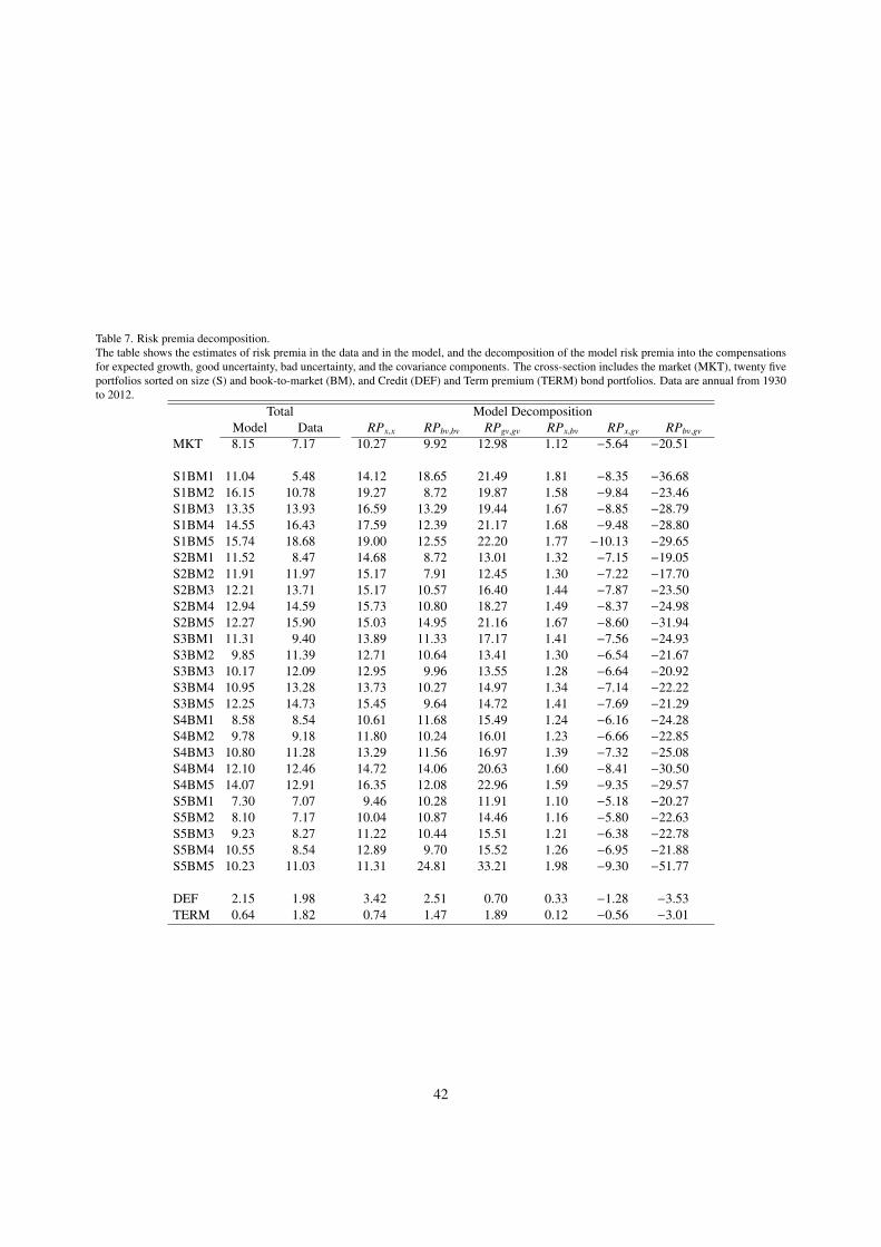
Table 7. Risk premia decomposition.The table shows the estimates of risk premia in the data and in the model, and the decomposition of the model risk premia into the compensationsfor expected growth, good uncertainty, bad uncertainty, and the covariance components. The cross-section includes the market (MKT), twenty fiveportfolios sorted on size (S) and book-to-market (BM), and Credit (DEF) and Term premium (TERM) bond portfolios. Data are annual from 1930to 2012.
Total Model DecompositionModel Data RPx,x RPbv,bv RPgv,gv RPx,bv RPx,gv RPbv,gv
MKT 8.15 7.17 10.27 9.92 12.98 1.12 −5.64 −20.51
S1BM1 11.04 5.48 14.12 18.65 21.49 1.81 −8.35 −36.68S1BM2 16.15 10.78 19.27 8.72 19.87 1.58 −9.84 −23.46S1BM3 13.35 13.93 16.59 13.29 19.44 1.67 −8.85 −28.79S1BM4 14.55 16.43 17.59 12.39 21.17 1.68 −9.48 −28.80S1BM5 15.74 18.68 19.00 12.55 22.20 1.77 −10.13 −29.65S2BM1 11.52 8.47 14.68 8.72 13.01 1.32 −7.15 −19.05S2BM2 11.91 11.97 15.17 7.91 12.45 1.30 −7.22 −17.70S2BM3 12.21 13.71 15.17 10.57 16.40 1.44 −7.87 −23.50S2BM4 12.94 14.59 15.73 10.80 18.27 1.49 −8.37 −24.98S2BM5 12.27 15.90 15.03 14.95 21.16 1.67 −8.60 −31.94S3BM1 11.31 9.40 13.89 11.33 17.17 1.41 −7.56 −24.93S3BM2 9.85 11.39 12.71 10.64 13.41 1.30 −6.54 −21.67S3BM3 10.17 12.09 12.95 9.96 13.55 1.28 −6.64 −20.92S3BM4 10.95 13.28 13.73 10.27 14.97 1.34 −7.14 −22.22S3BM5 12.25 14.73 15.45 9.64 14.72 1.41 −7.69 −21.29S4BM1 8.58 8.54 10.61 11.68 15.49 1.24 −6.16 −24.28S4BM2 9.78 9.18 11.80 10.24 16.01 1.23 −6.66 −22.85S4BM3 10.80 11.28 13.29 11.56 16.97 1.39 −7.32 −25.08S4BM4 12.10 12.46 14.72 14.06 20.63 1.60 −8.41 −30.50S4BM5 14.07 12.91 16.35 12.08 22.96 1.59 −9.35 −29.57S5BM1 7.30 7.07 9.46 10.28 11.91 1.10 −5.18 −20.27S5BM2 8.10 7.17 10.04 10.87 14.46 1.16 −5.80 −22.63S5BM3 9.23 8.27 11.22 10.44 15.51 1.21 −6.38 −22.78S5BM4 10.55 8.54 12.89 9.70 15.52 1.26 −6.95 −21.88S5BM5 10.23 11.03 11.31 24.81 33.21 1.98 −9.30 −51.77
DEF 2.15 1.98 3.42 2.51 0.70 0.33 −1.28 −3.53TERM 0.64 1.82 0.74 1.47 1.89 0.12 −0.56 −3.01
42

Tabl
e8.
Sim
ulat
ion
anal
ysis
ofm
acro
econ
omic
unce
rtai
ntie
san
dag
greg
ate
grow
th.
The
tabl
esh
ows
the
Mon
te-C
arlo
pred
icta
bilit
yev
iden
cefo
rthe
proj
ectio
nof
futu
reco
nsum
ptio
nan
ddi
vide
ndgr
owth
rate
son
the
curr
ente
xpec
ted
cons
umpt
ion
grow
thx,
good
unce
rtai
nty
Vg,
and
bad
unce
rtai
nty
Vb
:1 h∑ h j=
1∆
y t+
j=
a h+
b′ h[xt,
Vgt,V
bt]+
erro
r.T
heta
ble
repo
rts
the
popu
latio
nan
dsm
all-
sam
ple
estim
ates
(cor
resp
ondi
ngto
5%,5
0%an
d95
%pe
rcen
tile
ofth
edi
stri
butio
nin
sim
ulat
ions
)of
the
slop
eco
effici
ents
and
R2 s.
The
cons
umpt
ion,
divi
dend
s,an
das
setp
rice
sar
esi
mul
ated
onm
onth
lyfr
eque
ncy
and
aggr
egat
edto
annu
alho
rizo
nun
der
the
long
-run
risk
s,si
ngle
-vol
atili
tym
odel
confi
gura
tion
ofB
ansa
l,K
iku,
and
Yar
on(2
013)
.R
ealiz
edpo
sitiv
ean
dne
gativ
eva
rian
ces
are
cons
truc
ted
from
the
mod
el-s
imul
ated
dem
eane
dm
onth
lyco
nsum
ptio
ngr
owth
rate
over
the
year
.T
heex
-ant
eun
cert
aint
ym
easu
res
corr
espo
ndto
the
proj
ectio
nsof
the
log
real
ized
vari
ance
son
the
seto
fpr
edic
tors
,suc
has
real
ized
posi
tive
and
nega
tive
vari
ance
s,co
nsum
ptio
ngr
owth
,mar
ketr
etur
n,th
em
arke
t-pr
ice
divi
dend
ratio
,and
the
risk
-fre
era
te.
Smal
l-sa
mpl
eev
iden
ceis
base
don
100,
000
sim
ulat
ions
of83
year
sof
mon
thly
data
;th
epo
pula
tion
estim
ates
are
base
don
alo
ngsi
mul
atio
nof
1,00
0,00
0ye
ars
ofda
ta.
xV
bV
gR
2
Pop
5%M
ed95
%Po
p5%
Med
95%
Pop
5%M
ed95
%Po
p5%
Med
95%
Ben
chm
ark
Mod
el:
Con
sum
ptio
n:1Y
Ahe
ad1.
571.
222.
003.
008.
53-1
0.58
53.5
614
4.74
-9.5
6-1
47.4
1-5
6.91
8.67
0.41
0.24
0.42
0.59
3YA
head
1.03
0.64
1.02
1.41
1.19
-35.
101.
5739
.67
-1.6
1-3
8.30
-2.0
133
.39
0.36
0.16
0.38
0.60
5YA
head
0.78
0.24
0.67
1.13
0.24
-45.
65-2
.81
40.0
8-0
.53
-38.
342.
8044
.23
0.29
0.09
0.31
0.56
Div
iden
d:1Y
Ahe
ad3.
95-0
.47
5.37
12.7
619
.89
-480
.68
106.
3578
8.62
-51.
52-1
087.
24-2
82.1
025
4.73
0.09
0.01
0.14
0.33
3YA
head
2.57
-0.8
92.
686.
421.
71-3
57.8
2-2
.84
354.
48-1
2.72
-428
.53
-52.
3527
7.72
0.09
-0.0
10.
120.
355Y
Ahe
ad1.
96-1
.21
1.75
4.82
-0.2
0-3
04.4
6-1
1.11
277.
78-6
.72
-319
.33
-21.
0125
7.18
0.08
-0.0
20.
120.
38
Stra
ight
OL
SM
odel
:C
onsu
mpt
ion:
1YA
head
3.15
1.78
2.60
3.71
132.
9735
.13
115.
8324
1.12
-132
.80
-240
.56
-116
.93
-37.
910.
460.
260.
450.
623Y
Ahe
ad1.
001.
001.
001.
000.
00-0
.00
0.00
0.00
0.00
-0.0
00.
000.
000.
360.
150.
370.
595Y
Ahe
ad0.
580.
140.
570.
95-1
4.54
-56.
22-1
3.27
24.8
014
.52
-23.
9113
.59
55.9
40.
300.
080.
300.
56D
ivid
end:
1YA
head
12.2
9-2
.05
7.76
18.4
966
0.74
-782
.68
336.
7415
18.2
8-7
07.9
8-1
753.
33-5
45.0
552
8.96
0.13
0.01
0.16
0.36
3YA
head
3.96
-1.9
02.
867.
6710
9.97
-488
.25
9.05
503.
43-1
26.1
5-5
75.3
8-7
4.37
402.
160.
09-0
.01
0.11
0.34
5YA
head
2.33
-2.0
61.
605.
2129
.93
-406
.45
-28.
6732
9.97
-39.
86-3
70.3
9-8
.94
355.
170.
08-0
.02
0.11
0.37
AR
(1)A
djus
tmen
tMod
el:
Con
sum
ptio
n:1Y
Ahe
ad1.
571.
222.
002.
998.
88-9
.97
54.6
514
7.90
-9.8
3-1
49.6
1-5
8.09
8.32
0.41
0.23
0.42
0.59
3YA
head
1.02
0.64
1.01
1.41
1.12
-36.
221.
4339
.92
-1.5
0-3
8.38
-1.8
034
.87
0.36
0.16
0.38
0.60
5YA
head
0.78
0.24
0.67
1.13
0.12
-47.
10-3
.13
40.1
7-0
.30
-38.
213.
0945
.67
0.29
0.09
0.31
0.56
Div
iden
d:1Y
Ahe
ad3.
91-0
.48
5.35
12.7
119
.92
-492
.75
110.
3580
1.79
-50.
16-1
098.
71-2
85.9
726
7.96
0.09
0.01
0.14
0.33
3YA
head
2.54
-0.8
82.
676.
421.
95-3
65.1
6-3
.93
360.
27-1
2.12
-431
.43
-52.
9828
6.43
0.09
-0.0
10.
120.
355Y
Ahe
ad1.
92-1
.20
1.75
4.81
-0.3
5-3
10.8
3-1
2.29
282.
25-5
.62
-322
.12
-20.
9026
2.79
0.08
-0.0
20.
120.
38
43

Table 9. Model-implied significance of the volatility coefficients.The table shows the Monte-Carlo predictability evidence for the projection of future consumption and dividend growth rates on the current expectedconsumption growth x, good uncertainty Vg, and bad uncertainty Vb : 1
h∑h
j=1 ∆yt+ j = ah + b′h[xt ,Vgt ,Vbt] + error. The table reports the fractionof samples in which bad (good) uncertainty loadings at 1-, 3-, and 5-year maturities are all negative (positive). The data are simulated on monthlyfrequency and aggregated to annual horizon under the long-run risks, single-volatility model configuration of Bansal, Kiku, and Yaron (2013).Realized positive and negative variances are constructed from the model-simulated demeaned monthly consumption growth rate over the year.The ex-ante uncertainty measures correspond to the projections of the log realized variances on the set of predictors, such as realized positive andnegative variances, consumption growth, market return, the market-price dividend ratio, and the risk-free rate. Small-sample evidence is based on100,000 simulations of 83 years of monthly data.
Pr(bbv < 0) Pr(bgv > 0) Pr(bbv<0 & bgv > 0)Benchmark Model:
Consumption Growth: 0.05 0.04 0.03Dividend Growth: 0.24 0.12 0.09Joint: 0.02 0.01 0.01
Straight OLS Model:Consumption Growth: 0.004 0.004 0.002Dividend Growth: 0.21 0.13 0.11Joint: 0.002 0.001 0.001
AR(1) Adjustment Model:Consumption Growth: 0.05 0.04 0.03Dividend Growth: 0.24 0.12 0.09Joint: 0.02 0.01 0.01
44
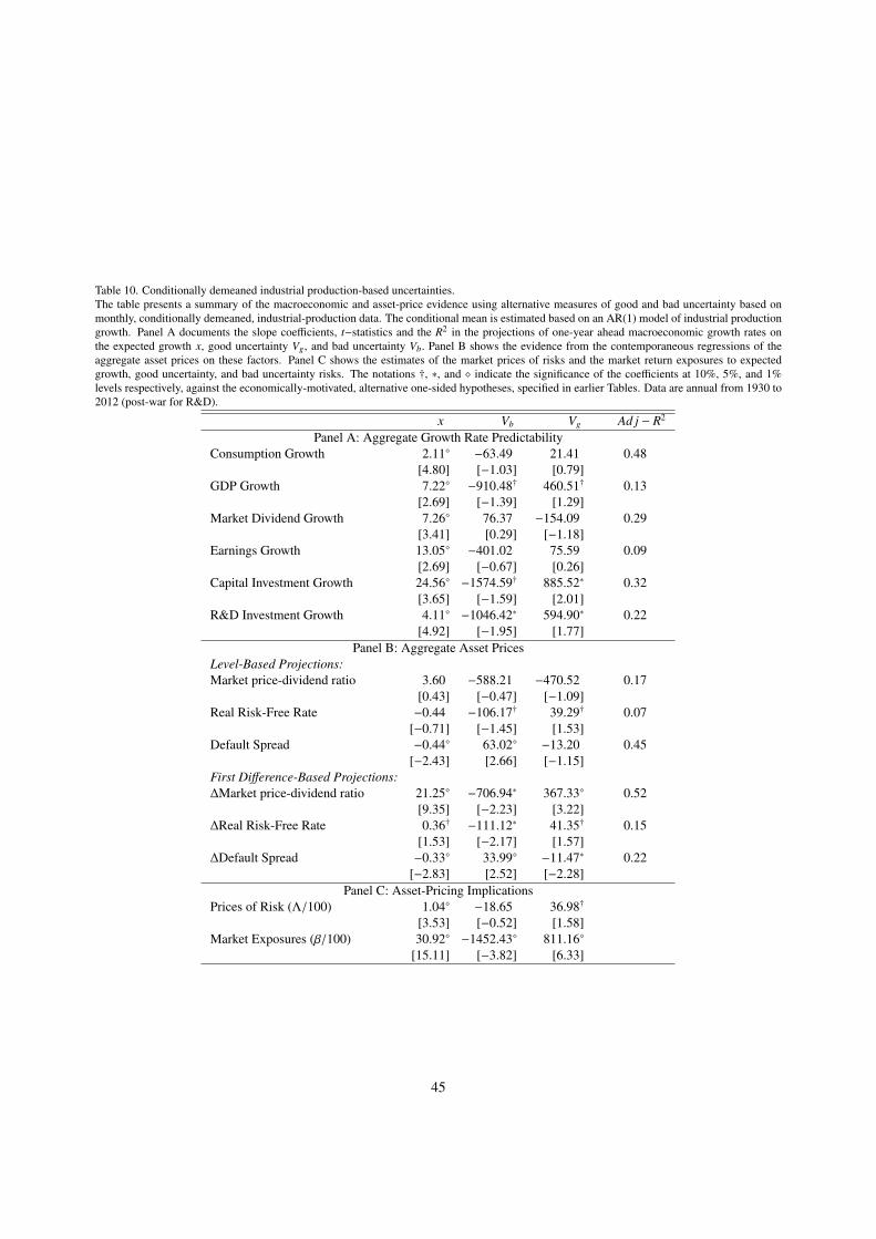
Table 10. Conditionally demeaned industrial production-based uncertainties.The table presents a summary of the macroeconomic and asset-price evidence using alternative measures of good and bad uncertainty based onmonthly, conditionally demeaned, industrial-production data. The conditional mean is estimated based on an AR(1) model of industrial productiongrowth. Panel A documents the slope coefficients, t−statistics and the R2 in the projections of one-year ahead macroeconomic growth rates onthe expected growth x, good uncertainty Vg, and bad uncertainty Vb. Panel B shows the evidence from the contemporaneous regressions of theaggregate asset prices on these factors. Panel C shows the estimates of the market prices of risks and the market return exposures to expectedgrowth, good uncertainty, and bad uncertainty risks. The notations †, ∗, and indicate the significance of the coefficients at 10%, 5%, and 1%levels respectively, against the economically-motivated, alternative one-sided hypotheses, specified in earlier Tables. Data are annual from 1930 to2012 (post-war for R&D).
x Vb Vg Ad j − R2
Panel A: Aggregate Growth Rate PredictabilityConsumption Growth 2.11 −63.49 21.41 0.48
[4.80] [−1.03] [0.79]GDP Growth 7.22 −910.48† 460.51† 0.13
[2.69] [−1.39] [1.29]Market Dividend Growth 7.26 76.37 −154.09 0.29
[3.41] [0.29] [−1.18]Earnings Growth 13.05 −401.02 75.59 0.09
[2.69] [−0.67] [0.26]Capital Investment Growth 24.56 −1574.59† 885.52∗ 0.32
[3.65] [−1.59] [2.01]R&D Investment Growth 4.11 −1046.42∗ 594.90∗ 0.22
[4.92] [−1.95] [1.77]Panel B: Aggregate Asset Prices
Level-Based Projections:Market price-dividend ratio 3.60 −588.21 −470.52 0.17
[0.43] [−0.47] [−1.09]Real Risk-Free Rate −0.44 −106.17† 39.29† 0.07
[−0.71] [−1.45] [1.53]Default Spread −0.44 63.02 −13.20 0.45
[−2.43] [2.66] [−1.15]First Difference-Based Projections:∆Market price-dividend ratio 21.25 −706.94∗ 367.33 0.52
[9.35] [−2.23] [3.22]∆Real Risk-Free Rate 0.36† −111.12∗ 41.35† 0.15
[1.53] [−2.17] [1.57]∆Default Spread −0.33 33.99 −11.47∗ 0.22
[−2.83] [2.52] [−2.28]Panel C: Asset-Pricing Implications
Prices of Risk (Λ/100) 1.04 −18.65 36.98†
[3.53] [−0.52] [1.58]Market Exposures (β/100) 30.92 −1452.43 811.16
[15.11] [−3.82] [6.33]
45

Table 11. Industrial production-based uncertainties with shifted cutoff.The table presents a summary of the macroeconomic and asset-price evidence using alternative measures of good and bad uncertainty based onmonthly industrial-production data, computed under a shifted cutoff for the good and bad uncertainty observations. The ex-post positive (negative)semivariance is computed using observations above (below) the 75th percentile of industrial production growth. Panel A documents the slopecoefficients, t−statistics and the R2 in the projections of one-year ahead macroeconomic growth rates on the expected growth x, good uncertaintyVg, and bad uncertainty Vb. Panel B shows the evidence from the contemporaneous regressions of the aggregate asset prices on these factors. PanelC shows the estimates of the market prices of risks and the market return exposures to expected growth, good uncertainty, and bad uncertainty risks.The notations †, ∗, and indicate the significance of the coefficients at 10%, 5%, and 1% levels respectively, against the economically-motivated,alternative one-sided hypotheses, specified in earlier Tables. Data are annual from 1930 to 2012 (post-war for R&D).
x Vb Vg Ad j − R2
Panel A: Aggregate Growth Rate PredictabilityConsumption Growth 2.01 −80.25† 16.91 0.52
[5.14] [−1.56] [1.09]GDP Growth 4.48 −680.39† 229.82† 0.05
[6.60] [−1.58] [1.50]Market Dividend Growth 8.78 −459.88∗ 38.09 0.40
[4.37] [−1.96] [0.50]Earnings Growth 12.26 −724.71 129.06 0.10
[3.58] [−1.19] [0.60]Capital Investment Growth 24.08 −2319.51∗ 830.56 0.38
[4.28] [−2.31] [2.65]R&D Investment Growth 4.39 −724.28 582.91∗ 0.28
[4.02] [−2.73] [2.31]Panel B: Aggregate Asset Prices
Level-Based Projections:Market price-dividend ratio 10.46 −3075.22 493.02† 0.24
[1.16] [−2.96] [1.49]Real Risk-Free Rate −0.02 −226.10∗ 73.65 0.19
[−0.03] [−2.14] [2.51]Default Spread −0.41 72.97 −10.93† 0.52
[−2.42] [4.30] [−1.40]First Difference-Based Projections:∆Market price-dividend ratio 18.54 −1588.31 445.77 0.61
[10.25] [−4.72] [3.58]∆Real Risk-Free Rate −0.01 −117.20† 28.81 0.14
[−0.06] [−1.53] [1.10]∆Default Spread −0.28 57.12 −14.03∗ 0.39
[−2.89] [3.13] [−2.21]Panel C: Asset-Pricing Implications
Prices of Risk (Λ/100) 0.94 −76.20∗ 37.39∗
[4.32] [−1.73] [2.06]Market Exposures (β/100) 24.39 −1642.30 560.40
[16.86] [−5.18] [4.19]
46

Table 12. Earnings-based uncertainties.The table presents a summary of the macroeconomic and asset-price evidence using alternative measures of good and bad uncertainty based onmonthly corporate earnings data. Panel A documents the slope coefficients, t−statistics and the R2 in the projections of one-year ahead macroeco-nomic growth rates on the expected growth x, good uncertainty Vg, and bad uncertainty Vb. Panel B shows the evidence from the contemporaneousregressions of the aggregate asset prices on these factors. Panel C shows the estimates of the market prices of risks and the market return exposuresto expected growth, good uncertainty, and bad uncertainty risks. The notations †, ∗, and indicate the significance of the coefficients at 10%, 5%,and 1% levels respectively, against the economically-motivated, alternative one-sided hypotheses, specified in earlier Tables. Data are annual from1930 to 2012 (post-war for R&D).
x Vb Vg Ad j − R2
Panel A: Aggregate Growth Rate PredictabilityConsumption Growth 1.86 −160.58∗ 41.10∗ 0.53
[7.10] [−2.00] [1.97]GDP Growth 4.86∗ −371.75 98.78 0.05
[2.00] [−2.73] [2.84]Market Dividend Growth 6.28 −1448.37 354.80 0.37
[3.01] [−3.99] [3.85]Earnings Growth 4.12 −1319.52† 166.00 0.21
[0.67] [−1.60] [0.86]Capital Investment Growth 18.98 −3498.01 901.57 0.43
[5.40] [−3.17] [3.21]R&D Investment Growth 2.63 720.54 −195.27 0.26
[2.72] [2.55] [−2.69]Panel B: Aggregate Asset Prices
Level-Based Projections:Market price-dividend ratio 2.38 −5282.53 1377.15 0.13
[0.37] [−2.59] [2.66]Real Risk-Free Rate −0.40 51.03 −24.48 −0.01
[−0.39] [0.25] [−0.44]Default Spread −0.08 76.82∗ −15.42 0.19
[−0.51] [1.68] [−1.26]First Difference-Based Projections:∆Market price-dividend ratio 16.81 −1688.33 399.38 0.61
[7.89] [−4.93] [4.48]∆Real Risk-Free Rate −0.44 −74.01∗ 12.36 0.05
[−0.96] [−2.02] [1.24]∆Default Spread −0.09 39.07† −6.31 0.44
[−1.15] [1.28] [−0.81]Panel C: Asset-Pricing Implications
Prices of Risk (Λ/100) 0.46 −238.78 69.48
[1.24] [−3.32] [3.19]Market Exposures (β/100) 25.68 −1502.40 401.75
[13.54] [−6.92] [7.49]
47

Table 13. Benchmark uncertainties: post-war sample.The table presents a summary of the macroeconomic and asset-price evidence using the benchmark uncertainty measures in the post-war period.Panel A documents the slope coefficients, t−statistics and the R2 in the projections of one-year ahead macroeconomic growth rates on the expectedgrowth x, good uncertainty Vg, and bad uncertainty Vb. Panel B shows the evidence from the contemporaneous regressions of the aggregate assetprices on these factors. Panel C shows the estimates of the market prices of risks and the market return exposures to expected growth, gooduncertainty, and bad uncertainty risks. The notations †, ∗, and indicate the significance of the coefficients at 10%, 5%, and 1% levels respectively,against the economically-motivated, alternative one-sided hypotheses, specified in earlier Tables. Data are annual from 1947 to 2012.
x Vb Vg Ad j − R2
Panel A: Aggregate Growth Rate PredictabilityConsumption Growth 1.43 −275.72 123.23 0.41
[6.27] [−3.57] [2.88]GDP Growth 2.27† −1127.75 1174.93∗ 0.44
[1.33] [−2.41] [2.09]Market Dividend Growth 2.41 −362.83 136.85 −0.01
[1.26] [−0.59] [0.51]Earnings Growth 11.39∗ −1941.22 666.54 0.02
[1.78] [−0.77] [0.67]Capital Investment Growth 8.33 −2231.30 1813.75 0.42
[3.45] [−4.51] [3.88]Panel B: Aggregate Asset Prices
Level-Based Projections:Market price-dividend ratio −5.92 −3987.38† −1011.95 0.34
[−0.65] [−1.59] [−0.75]Real Risk-Free Rate 1.32 −440.50 80.05 0.37
[3.04] [−2.35] [1.12]Default Spread −0.41 113.33∗ −49.41∗ 0.33
[−3.15] [1.66] [−2.11]First Difference-Based Projections:∆Market price-dividend ratio 20.93 −2740.74 665.55 0.61
[12.62] [−4.31] [2.70]∆Real Risk-Free Rate 0.37 −364.57 174.82 0.46
[1.09] [−3.39] [5.60]∆Default Spread −0.40 122.58 −4.44 0.61
[−3.63] [2.99] [−0.77]Panel C: Asset-Pricing Implications
Prices of Risk (Λ/100) 0.82 −74.95 38.15
[4.87] [−2.81] [3.43]Market Exposures (β/100) 28.84 −2912.56 938.32
[11.35] [−4.74] [2.57]
48

1930 1940 1950 1960 1970 1980 1990 2000 20100
0.5
1
1.5
2
2.5
3
3.5
4
x 10−3
Fig. 1. Total realized variance. The figure shows the time series plot of the total realized variance smoothed over a 3-year window. The totalrealized variance is based on the sum of squared observations of demeaned monthly industrial production growth over 1-year, re-scaled to matchthe unconditional variance of consumption growth. The shaded areas represent NBER recessions.
1930 1940 1950 1960 1970 1980 1990 2000 2010
−5
0
5
10
15
x 10−4
Fig. 2. Residual positive variance. The figure shows the time series plot of the residual positive variance, smoothed over a 3-year window, whichis orthogonal to the negative variance. The positive and negative realized semivariances decompose the total realized variance into the componentspertaining only to positive and negative movements in industrial production growth, respectively. The residual positive variance is computed fromthe projection of the positive realized semivariance onto the negative one. The shaded areas represent NBER recessions.
49

1930 1940 1950 1960 1970 1980 1990 2000 2010−13
−12
−11
−10
−9
−8
−7
−6
log(RV
p,t−3→ t)
log(Vg,t
)
1930 1940 1950 1960 1970 1980 1990 2000 2010−13
−12
−11
−10
−9
−8
−7
−6
log(RVn,t−3→ t)
log(Vb,t)
Fig. 3. Realized and predictive log volatilities. The figure shows the time series plots of the log positive (left Panel) and negative (right Panel)realized variances and their predictive values from the projection. The shaded areas represent NBER recessions. The benchmark predictive variablesin the projection include positive and negative realized semivariances, consumption growth rate, the real-market return, the market price-dividendratio, the real risk-free rate, and the default spread.
1930 1940 1950 1960 1970 1980 1990 2000 20100
0.5
1
1.5
2
2.5
x 10−3
Fig. 4. Total ex-ante uncertainty. The figure shows the time series plot of the total ex-ante uncertainty. The total ex-ante uncertainty is constructedfrom the predictive regressions of future overall realized variance. The shaded areas represent NBER recessions.
50

1930 1940 1950 1960 1970 1980 1990 2000 2010−4
−2
0
2
4
6
8
x 10−4
Fig. 5. Residual good uncertainty. The figure shows the time series plot of the residual good uncertainty which is orthogonal to the bad uncertainty.The good and bad uncertainties are constructed from the predictive regressions of future realized positive and negative variances, respectively. Theresidual good uncertainty is computed from the projection of good uncertainty onto bad uncertainty. The shaded areas represent NBER recessions.
51

(a) GDP Growth Response to Good Uncertainty Shock
0 2 4 6 8 10−1.5
−1
−0.5
0
0.5
1
1.5
2
2.5
(%)
(b) GDP Growth Response to Bad Uncertainty Shock
0 2 4 6 8 10
−1.2
−1
−0.8
−0.6
−0.4
−0.2
0
0.2
(%)
(c) GDP Growth Response to Total Uncertainty Shock
0 2 4 6 8 10
−0.2
−0.1
0
0.1
0.2
0.3
0.4
0.5
(%)
Fig. 6. Impulse response of GDP to macro uncertainties. The figure shows impulse responses of private GDP growth to one-standard deviationgood, bad, and total uncertainty shocks. The impulse responses are computed from a VAR(1) which includes macroeconomic uncertainty measures(bad and good uncertainty for the first two panels, and total uncertainty for the last panel), expected consumption growth, and GDP growth rate.Data are annual from 1930 to 2012.
52

(a) Capital Investment Growth Response to Good Uncertainty Shock
0 2 4 6 8 10
−1
−0.5
0
0.5
1(%
)
(b) Capital Investment Growth Response to Bad Uncertainty Shock
0 2 4 6 8 10−3
−2.5
−2
−1.5
−1
−0.5
0
0.5
(%)
(c) Capital Investment Growth Response to Overall Uncertainty Shock
0 2 4 6 8 10
−2
−1.5
−1
−0.5
0
0.5
1
(%)
Fig. 7. Impulse response of capital investment to macro uncertainties. The figure shows impulse responses of capital investment growth to one-standard deviation good, bad, and total uncertainty shocks. The impulse responses are computed from a VAR(1) which includes macroeconomicuncertainty measures (bad and good uncertainty for the first two panels, and total uncertainty for the last panel), expected consumption growth, andcapital investment growth rate. Data are annual from 1930 to 2012.
53

(a) R&D Investment Growth Response to Good Uncertainty Shock
0 2 4 6 8 10−0.1
0
0.1
0.2
0.3
0.4
0.5
0.6
0.7
(%)
(b) R&D Investment Growth Response to Bad Uncertainty Shock
0 2 4 6 8 10−1.2
−1
−0.8
−0.6
−0.4
−0.2
0
0.2
0.4
0.6
(%)
(c) R&D Investment Growth Response to Overall Uncertainty Shock
0 2 4 6 8 10
−0.6
−0.4
−0.2
0
0.2
0.4
0.6
(%)
Fig. 8. Impulse response of R&D investment to macro uncertainties. The figure shows impulse responses of R&D investment growth to one-standard deviation good, bad, and total uncertainty shocks. The impulse responses are computed from a VAR(1) which includes macroeconomicuncertainty measures (bad and good uncertainty for the first two panels, and total uncertainty for the last panel), expected consumption growth, andR&D investment growth rate. Data are annual from 1954 to 2008.
54

(a) Price-Dividend Ratio Response to Good Uncertainty Shock
0 2 4 6 8 10−0.01
0
0.01
0.02
0.03
0.04
0.05
0.06
0.07
(b) Price-Dividend Ratio Response to Bad Uncertainty Shock
0 2 4 6 8 10−0.06
−0.05
−0.04
−0.03
−0.02
−0.01
0
(c) Price-Dividend Ratio Response to Overall Uncertainty Shock
0 2 4 6 8 10
−0.04
−0.03
−0.02
−0.01
0
0.01
Fig. 9. Impulse response of price-dividend ratio to macro uncertainties. The figure shows impulse responses of the market price-dividend ratioto one-standard deviation good, bad, and total uncertainty shocks. The impulse responses are computed from a VAR(1) which includes macroe-conomic uncertainty measures (bad and good uncertainty for the first two panels, and total uncertainty for the last panel), expected consumptiongrowth, and the market price-dividend ratio. Data are annual from 1930 to 2012.
55

(a) Price-Earnings Ratio Response to Good Uncertainty Shock
0 2 4 6 8 10−0.01
0
0.01
0.02
0.03
0.04
(b) Price-Earnings Ratio Response to Bad Uncertainty Shock
0 2 4 6 8 10−0.035
−0.03
−0.025
−0.02
−0.015
−0.01
−0.005
0
(c) Price-Earnings Ratio Response to Overall Uncertainty Shock
0 2 4 6 8 10
−10
−8
−6
−4
−2
0
2
4x 10
−3
Fig. 10. Impulse response of price-earnings ratio to macro uncertainties. The figure shows impulse responses of the market price-earnings ratioto one-standard deviation good, bad, and total uncertainty shocks. The impulse responses are computed from a VAR(1) which includes macroe-conomic uncertainty measures (bad and good uncertainty for the first two panels, and total uncertainty for the last panel), expected consumptiongrowth, and the market price-earnings ratio. Data are annual from 1930 to 2012.
56