Good-Bye Lenin (Or Not?): The Effect of Communism on

Good-Bye Lenin (Or Not?): The Effect ofCommunism on People's Preferences

The Harvard community has made thisarticle openly available. Please share howthis access benefits you. Your story matters

Citation Alesina, Alberto, and Nicola Fuchs-Schündeln. 2007. Good-byeLenin (or not?): the effect of Communism on people's preferences.American Economic Review 97(4): 1507-1528.

Published Version doi:10.1257/aer.97.4.1507

Citable link http://nrs.harvard.edu/urn-3:HUL.InstRepos:4553032

Terms of Use This article was downloaded from Harvard University’s DASHrepository, and is made available under the terms and conditionsapplicable to Other Posted Material, as set forth at http://nrs.harvard.edu/urn-3:HUL.InstRepos:dash.current.terms-of-use#LAA

http://osc.hul.harvard.edu/dash/open-access-feedback?handle=&title=Good-Bye%20Lenin%20(Or%20Not?):%20The%20Effect%20of%20Communism%20on%20People's%20Preferences&community=1/1&collection=1/2&owningCollection1/2&harvardAuthors=c436ce1fb864525d3a821b6f91db789f&departmentEconomics

http://nrs.harvard.edu/urn-3:HUL.InstRepos:4553032

http://nrs.harvard.edu/urn-3:HUL.InstRepos:dash.current.terms-of-use#LAA



HH II EE RR

Harvard Institute of Economic Research

Discussion Paper Number 2076

Good bye Lenin (or not?): The effect of Communism on people’s

preferences

by

Alberto Alesina and Nicola Fuchs-Schundeln

July 2005

Harvard University Cambridge, Massachusetts

This paper can be downloaded without charge from: http://post.economics.harvard.edu/hier/2005papers/2005list.html

The Social Science Research Network Electronic Paper Collection:

http://ssrn.com/abstract=756786

Good bye Lenin (or not?):The effect of Communism on people’s

preferences∗

Alberto Alesina and Nicola Fuchs-SchündelnHarvard University

This version: June 2005

AbstractPreferences for redistribution, as well as the generosities of welfare

states, differ significantly across countries. In this paper, we test whetherthere exists a feedback process of the economic regime on individual prefer-ences. We exploit the experiment of German separation and reunificationto establish exogeneity of the economic system. From 1945 to 1990, EastGermans lived under a Communist regime with heavy state interventionand extensive redistribution. We find that, after German reunification,East Germans are more in favor of redistribution and state interventionthan West Germans, even after controlling for economic incentives. Thiseffect is especially strong for older cohorts, who lived under Communismfor a longer time period. We find that East Germans’ preferences convergetowards those of West Germans, and we calculate that it will take one totwo generations for preferences to converge completely.

1 IntroductionPreferences for redistribution and redistributive policies differ significantly acrosscountries.1 Are the regimes different solely because of different initial prefer-ences for redistribution in the populations? Or is there a feedback effect fromthe regime on preferences? Is it possible that living under a specific system leadsto adaptation of preferences?2 To put it more bluntly: are individual preferences∗We thank Matthias Schündeln and Andrei Shleifer for conversations, participants in a

seminar at Harvard for comments, and Antonia Attanassova and Francesco Trebbi for excellentresearch assistantship. Alesina gratefully acknowledges financial support from the NSF witha grant through the NBER.

1For instance, the difference between Europe and the US has been discussed recently byAlesina and Glaeser (2004).

2 Several recent theoretical papers have shown that there is scope for multiple equilibriaand self-fulfilling beliefs, i.e. that preferences influence the regime, and that the regime hasa feedback on preferences (see e.g. Piketty 1995, Alesina and Angeletos 2005, and Benabouand Tirole 2005).

1

endogenous to political regimes? In order to answer this question empirically,one needs an exogenous shock to the regime; post war Germany offers an oppor-tunity to analyze the effect of one particular regime, Communism, on people’spreferences.From 1945 to 1990, Germany was split into two parts for reasons that had

nothing to do with Germans’ desire for separation, or diversity of visions be-tween East Germans and West Germans: the division of Germany into twoparts was exogenous with respect to underlying individual preferences. Sincethe political and economic system has been the same in the eastern and westernparts of Germany since reunification in 1990, and was the same before 1945,West Germans constitute a meaningful control group for East Germans. There-fore, comparing the differences in attitudes and preferences of Germans afterthe reunification can give us a clue about the effects of living for 45 years undera Communist regime on attitudes, beliefs and political preferences.We are especially interested in measuring how 45 years of Communism af-

fected individuals’ thinking toward market capitalism and the role of the statein providing welfare and redistribution from the rich to the poor. If politicalregimes had no effects on individual preferences one should not observe anysystematic difference between East and West Germans after reunification. IfCommunism had an effect, in principle one could think of two possible reac-tions to 45 years of Communist dictatorship. One is that people turn stronglyagainst the “state” and switch to preferences in the opposite direction, namelyin favor of liberitarian free markets, as a reaction to an all intrusive state. Theopposite hypothesis is that 45 years of heavy state intervention and indoctrina-tion instill in people the view that the state is essential for individual well being.As we shall see, we quickly and soundly reject the first hypothesis in favor ofthe second. In fact, we find that the effects of Communism are large and longlasting. It will take about one to two generations for former East and WestGermans to look alike in terms of preferences and attitudes about fundamentalquestions regarding the role of the government in society.There can be two effects of Communism on individual preferences, namely

a purely economic one, and an effect on intrinsic preferences. The latter couldarise because of Marxist Leninist indoctrination, state control over school, press,or state television, etc. Also, simply becoming accustomed to an all encompass-ing state may make people think of it as necessary and preferable despite thesuffocating aspects of the East German regime. This is the effect we are mostinterested in. The former effect arises because Communism has made formerEast Germany relatively poorer than former West Germany. Since the poordisproportionately benefit from government redistribution, they favor it. Wefind evidence of both types of effect.We also investigate “why” former East Germans are more likely to favor state

intervention. One reason is that they are simply used to it. Another reasonis that East Germans believe much more so than West Germans that socialconditions, rather than individual effort and initiative, determine individualfortunes; this belief is of course one basic tenet of the communist ideology. Themore one thinks that it is society’s “fault” if one is poor, unemployed or sick,

2

the more one is in favor of public intervention. We find evidence for both effects.Last, we analyze whether preferences of East Germans converge towards

those of West Germans, given that they now live under the same regime WestGermans have experienced since 1945. We calculate that it will take about 20to 40 years to make the difference between East and West Germans disappearalmost completely, due to the combination of two forces. One is the dying ofthe elderly and the coming of age of individuals born after reunification; theother is the actual change of preferences of the same individuals. We estimatethe first effect to account for about 1/3 of the convergence effect and the otherone to account for the remaining 2/3 of the convergence.An implication of all of the above is that Germany in 1990 has been subject

to a major political shock, perhaps with deeper and longer lasting consequencesthan the widely studied economic shock associated with the reunification. Acountry like former West Germany with an already generous welfare state, heavylabor and goods market regulations etc., which many believe needs trimming,has received a new 25 per cent of population inclined to prefer an even moreextensive role for the state, even after controlling for them being on averagenet recipients of government intervention. This will make any political reformtowards trimming the welfare state (broadly defined) especially difficult. All ofthose who believe that the economic future of Germany (which looks somewhatbleak at the moment) will look brighter with a host of so called “structuralreforms” should be especially concerned.3

The question of preferences for redistribution and different visions about thewelfare state has recently received much attention. Alesina and Glaeser (2004)discuss the origin of different beliefs and preferences in the US and ContinentalWestern Europe, and in fact place a lot of weight on the influence of Marxistideology on the preference for redistribution in Europe versus the US. Alesinaand La Ferrara (2005) and Fong (2003) investigate the connection about viewsabout social mobility and preferences for redistribution using US data. Ravallionand Lokshin (2000) consider Russian data. In general, this literature finds thatthe more individuals perceive that there is social mobility the less favorable theyare to government redistribution.The paper most closely related to ours is Corneo (2001). Building on Cor-

neo and Grüner (2002), he studies empirically what motivates individuals tofavor redistribution, from purely individual to altruistic motives. In examiningthis issue, Corneo (2001) compares preferences in the US, West Germany andEast Germany. One of his results is that East Germans are more favorableto redistribution than West Germans, who, in turn, are more favorable to itthan Americans. More generally, in a comparison of 6 Eastern European and 6Western countries, Corneo and Grüner (2002) find large country fixed effects forEastern European countries; i.e. they find that Eastern Europeans have strongerpreferences for redistribution than individuals from Western countries.4 Corneo

3Giavazzi and McMahon (2005) have recently pointed out how the German reform processin fact is lacking political support from the people.

4Besides East Germany, their sample includes Hungary, Czechoslovakia, Poland, Romania,and Russia.

3

(2001) as well as Corneo and Grüner (2002) use data from the 1992 round of theInternational Social Survey Programme. We can expand on their analyses sincewe use a panel data set. By using different waves of our data, we can discussmore precisely timing issues and speed of convergence of preferences.5 Moreover,we can include many more individual controls. Last, by focusing on Germany,we can distinguish more clearly the role of Communism in shaping preferencesfrom other potential reasons why Eastern Europeans might favor redistribution.That is, it could be that preferences in Eastern Europe are different because ofdifferent cultures, histories etc. even before the advent of Communism. More-over, a more uncertain environment and absence of insurance markets couldinduce Eastern Europeans to favor redistribution.The paper is organized as follows. In Section 2 we describe the institutional

background, data and summary statistics. In Section 3 we present our basic re-sults concerning preferences for state intervention in social policy. This sectionbreaks down effects on preferences emerging from relative poverty in the Eastfrom the pure preference effect of communism. In Section 4 we investigate re-lated attitudes about individual responsibility versus social conditions that canexplain differences in preferences regarding the welfare state. The last sectionconcludes.

2 Institutional Background, Data and SummaryStatistics

2.1 Institutional Background

Germany as a country was created in 1860 as a result of the political unificationof 18 independent political units of various size, the largest and most powerfulbeing Prussia. Germany remained a single country until the end of the SecondWorldWar when, as a losing power, it was split amongst the winning Allies. EastGermany was under the sphere of influence of the Soviets, while the West wasoccupied by the US, France, and the UK. The borders between East and WestGermany were the result of bargaining between the Allies and the position ofthe occupying forces at the end of hostilities. In 1949, both the Federal Republicof Germany (FRG) and the German Democratic Republic (GDR) were officiallyfounded. The East German regime developed as one of the most rigid of theformer Communist regimes. Income inequality in the GDR was low: in 1988,the average net income of individuals with a university degree was only 15%higher than that of blue collar workers, compared to 70% in the FRG. Also,intersectoral differences in net incomes were minimal, on average amounting

5 In addition, we can also check whether West Germans are becoming more or less in favorof the welfare state, an intriguing question given the recent attempt of the German governmentto implement ”structural reforms”, a buzz word for pro market reforms. The political support(or lack thereof) of such reforms is the result of the ”political shock” associated with thearrival of new preferences for Easterners and the evolution of preferences of Westeners. Ourconclusions will not give much hope to those who see pro market reforms as desirable.

4

only to 150 Mark per month with an average monthly income of around 1100Mark in 1988 (Stephan and Wiedemann, 1990, Schäfgen, 1998). Reunificationoccurred rather quickly and abruptly in October 1990, 11 months after the fallof the Berlin Wall in November 1989. East Germany became part of the FederalRepublic of Germany, and hence the economic and political system of the Westwas transferred to the East.One important identifying assumption of our analysis is that East and West

Germany were indistinguishable until the exogenously imposed separation in1945. Because of this, if we observe differences in attitudes amongst East andWest Germans after reunification, we can attribute them to 45 years of Com-munism. How reasonable is the assumption that East and West Germans wereindistinguishable in terms of their attitudes before 1945? Table 1 shows averageper capita income levels of different German regions, as well as subregions ofPrussia, in 1928, 1932, and 1936. We mark a region by E or W, dependingon whether it mainly belonged to the FRG or GDR between 1949 and 1990.Unmarked regions do not belong to Germany after 1945.6 As the table shows,the level of income per capita in pre-World War II Germany does not showany systematic difference between East and West; in fact, on average they arealmost identical.7 Moreover, destruction during World War II was major anduniversal in both the later FRG and GDR.However, income per capita aside, there might have been differences in atti-

tudes before 1945. One possible issue is that Prussians might have had a moremilitarist ”state-centric” view about the state than other Germans. Note how-ever that part of former Prussia belonged to the FRG and part to the GDRbetween 1949 and 1990, and not all regions of the later GDR belonged to Prus-sia.

2.2 The Data

The German Socioeconomic Panel (GSOEP) is an annual household panel,started in West Germany in 1984. From 1990 on, it also covers the territoryof the former German Democratic Republic. We use the original sample estab-lished in 1984, and the sub-sample covering the territory of the former GDRstarted in 1990. The original West German sample leaves us with around 11,400year-person observations, while the East German sample covers around 7,000year-person observations for 1997 and 2002.8

In 1997 and 2002, respondents were asked questions concerning their prefer-ences for the role of the state in different areas of social security. The questionreads: “At present, a multitude of social services are provided not only by thestate but also by private free market enterprises, organizations, associations, or

6Note that some regions transcend later borders, in which case we assign the region toEast, West or outside Germany depending on its largest share.

7The non-population weighted average income in later East regions amounted to 1,203Mark in 1928, 877 Mark in 1932, and 1,169 Mark in 1936, while the corresponding incomesfor the later West regions are 1,203, 913, and 1,200 Mark.

8The number of observations varies slightly with the dependent variable.

5

private citizens. What is your opinion on this? Who should be responsible forthe following areas?”. We use the answers to all areas that concern financial se-curity, namely “financial security in case of unemployment”, “financial securityin case of illness”, “financial security of families”, “financial security for old-age”, and “financial security for persons needing care”. The answers are givenon a scale of 1 to 5, which correspond to “only the state”, “mostly the state”,“state and private forces”, “mostly private forces”, and “only private forces”.We group the first 2 answer categories together to represent individuals withpreference for an active role of the state in providing for its citizens, and groupthe last 3 answer categories together to represent individuals with preferencesfor private forces. Hence, we create 5 new dummy variables which take on thevalue of 1 if the respondent answered “only the state” or “mostly the state” forthe respective area, and 0 otherwise. This is mainly done to ease the interpreta-tion of the coefficients. As a robustness check, we run ordered probit regressionson the original variables, and the results do not change significantly.9

Our explanatory variable of main interest is an East dummy that takes onthe value of 1 if the respondent lived in East Germany before reunification,regardless of the current place of residence. Hence, this dummy captures peoplewho lived under communism before 1990. The baseline controls include age,gender, marital status, labor force status, and occupation of the respondent,the number of children and the number of adults in the household, as well asthe annual household income. All monetary variables are in DM and inflatedto 2002.We analyze two additional questions that capture the belief of the respon-

dent regarding important driving forces of success in life. In 1996 and 1999,GSOEP asked the following question: “The following statements express vary-ing attitudes towards life and the future. Please state whether you totally agree,agree slightly, disagree slightly, or totally disagree”, followed by several state-ments that differ between 1996 and 1999. The first statement we use refers tothe role of luck in life. We create a dummy variable “luck” that takes on thevalue of 1 if the respondent agreed totally or slightly with the statements “Noone can escape their fate, everything in life happens as it must happen” in 1996and “What one achieves in life is mainly a question of luck or fate” in 1999.10

Similarly, the dummy variable ”social conditions” takes on the value 1 if therespondent agreed totally or slightly with the statement “The possibilities inmy life are determined by the social conditions”.11

2.3 Summary Statistics

Table 2 reports the basic summary statistics regarding the five questions that weuse as dependent variables.12 This cross tabulation already highlights several

9The basic results using ordered probits are shown in Table A2 in Appendix. All otherresults are available from the authors upon request.10We take the average of both questions to alleviate potential measurement error.11This question was asked in 1999. There is no equivalent statement in 1996.12Table A1 in the appendix shows summary statistics for all independent variables.

6

important facts. First, a larger proportion of East Germans than West Germansfavor an active role of the state. The difference is substantial in all categories.Second, in 2002 East and West Germans looked more alike than in 1997. TheEast-West difference in the percentage of individuals favoring an active staterole amounts to between 16 and 18 percentage points in 1997, and between 9and 14 percentage points in 2002. Third, this convergence arises mostly fromchanging preferences of East Germans. In all questions, the percentage of EastGermans favoring an active role of the state is declining between 1997 and 2002.Last, and this is somewhat more surprising, the support of West Germans forthe welfare state is increasing between 1997 and 2002 in 3 out of the 5 categories,namely regarding unemployment, sickness, and care.This table also reports summary statistics for the two questions concerning

beliefs about what determines success in life, namely individual effort againstluck and/or social conditions. The interesting finding here is that East Germansare overwhelmingly convinced that social conditions determine success, more sothan West Germans. Moreover, they believe less than West Germans in animportant role of luck. In other words, East Germans seem to believe muchmore than West Germans that somebody’s life is defined by social conditions,a basic tenet of the Marxist way of thinking.Table 3 shows the income per capita and the unemployment rates in German

states (Bundesländer), as well as transfers per capita that each state receivesfrom other states and the federal government in line with the German financialtransfer system (see the appendix for an overview of the German transfer sys-tem). Average income per capita in the East is around 80% of the average Westincome, and the unemployment rate is roughly twice as large. As we discussedabove, before WWII per capita income levels in East and West Germany werevirtually identical. The 20 percent difference in per capita income after reunifi-cation can be interpreted as the effect of communism on economic development.The lower income levels as well as the higher unemployment rates lead to thefact that all Eastern German states are net recipient of transfers. Among theWestern German states, five are net givers, while four are net recipients. Yet,with the exception of the small state of Bremen, the average transfer receivedis much larger in the East than among the net recipients in the West.

3 Basic ResultsTable 4 reports our basic specifications, in which we control for many individualcharacteristics and for our variable of interest, being from the East. As wediscussed above, the left hand side variable is defined as a 0/1 variable with 1meaning support for an active state role. We also rerun all these regressionsusing the entire five point scale, and the results are consistent. Table A2 inthe appendix is the same as Table 4, but the left hand side variable has thefive point scale, and an ordered probit estimation is conducted. In the maintext, we report the results from probit regressions for ease of interpretation.The coefficients reported in the tables are the total coefficients. We report the

7

corresponding marginal coefficients in the text when we are interpreting thesize of the coefficients. The marginal coefficients of interaction variables arecalculated as the cross partial derivatives (Ai and Norton, 2003).The first three explanatory variables are the critical ones; and for all the five

questions they behave similarly. Consider column 1, which concerns unemploy-ment. An East German is significantly more likely to have preferences for stateprovision of financial security for the unemployed than a West German. Overtime, however, the East Germans are becoming less pro state, since the interac-tion between being from the East and the 2002 dummy (the third variable) isnegative and statistically significant. The effect of being an East German andthe interaction of that with 2002 have similar coefficients on all questions. Thecoefficients on the East indicator variable vary from 0.36 to 0.41, and are hencerather uniform. The interaction of East with 2002 (a rough measure of con-vergence) varies from -0.06 to -0.18. The economic meaning of these numbersis as follows.13 Being from the East increases the probability of favoring stateintervention by between 14 and 16 percentage points in 1997, compared to beingfrom the West. Between 1997 and 2002, the probability of favoring state inter-vention for an East German declines by between 2.5 and 5.8 percentage points.Given that these questions are reported at a 5 year interval (1997 and 2002), avery rough measure of convergence would imply full uniformity of views from aminimum of about 15 years (column 5) to a maximum of 30 years in column 3.Given that the first survey was taken 7 years after reunification, the completecycle of convergence (assuming that it is linear) would be between roughly 20and 40 years, depending on the question; roughly one to two generations.14

The dummy for 2002 captures the change in preferences of a West Germanbetween 1997 and 2002. Note that it is significantly positive, indicating thatWesterners are becoming more pro government, for 3 of the 5 regressions. Innone of the five regressions is there significant evidence that West Germans arebecoming less pro government.The estimates on individual controls yield reasonable results. Men are gen-

erally less pro government (although not consistently on all questions). Largerfamilies, both in terms of number of children and number of adults, are morefavorable to government intervention, not surprisingly, since they get more ben-efits. Interestingly, civil servants have weaker preferences than others for gov-ernment intervention for the unemployed, probably because they have very highjob security. On the contrary, those who are unemployed strongly prefer govern-ment intervention for unemployed. Income enters negatively and is statisticallysignificant on all questions; the wealthy benefit less from government interven-tion and pay more for it. Self employed are less pro government either because

13The marginal effect on y of a dummy variable x has been calculated as E [y|x = 1] −E [y|x = 0].14Our results are based on unweighted observations. If we use the sample weights provided

by GSOEP, the results are very similar. The only difference worth mentioning is that theconvergence results become weaker, indicating an even longer process of convergence. However,when we include wealth variables as controls (as described at the end of this section), theconvergence results are again very similar to the unweighted results.

8

they benefit less from redistribution, or because being self employed is correlatedwith a more individualistic vision of the world and/or with less risk aversion.15

All these variables are always included in all our regressions and the coefficientsare quite stable. From now on, we do not report them to avoid cluttering thetables.Our data set also includes two variables which proxy for wealth. One is

the amount of interest and dividend income obtained by the household of therespondent; the second is whether or not the household owns the house it livesin. When we add these variables in the regressions of Table 4, our results onthe East-West differences remain virtually unchanged, and the coefficients onthe two wealth variables have the expected sign and are statistically significant.These results are reported in table A3 in the appendix. We do not include thesetwo wealth controls in our basic regressions because of data availability. Afterthe inclusion of these variables, we lose around 2,200 observations because ofnon respondence. For robustness, we checked all our results including these twovariables, in addition to those of Table 4, and the results are robust. Theseresults are available upon request.

3.1 Age effects

Let us now consider more closely the effects of the number of years under Com-munism on individual preferences. Table 5 shows some striking results. Considercolumn 1.16 The variable “age” corresponds to the age of the respondent. TheEast indicator variable interacted with age is positive, meaning that older formerEast Germans are more favorable to state intervention. Note how age not inter-acted with East is negative, meaning that West Germans are becoming less progovernment as they become older, the same result found for the US by Alesinaand La Ferrara (2005).17 The effect of age on preferences is exactly opposite inEast and West. The same pattern applies to all other questions. The obviousinterpretation of this strikingly different age patterns between East Germansand West Germans is that while age tends to make individuals less pro govern-ment in West Germany, this effect is more than compensated by the fact thatelderly East Germans have lived longer under communism.Table 6 pushes this age analysis further by looking at five different groups

of birth cohort. The five groups are defined as follows: youngest are those bornafter 1975, young are those born between 1961 and 1975, middle are those bornbetween 1946 and 1960, old are those born between 1931 and 1945, and oldestare those born on or before 1930. Note that the youngest group did only spendtheir childhood and early adolescence under communism; this is the omittedgroup in the regressions. This table shows that the older are progressively15All these results on individual controls are qualitatively similar to those obtained for the

US by Alesina and La Ferrara (2005).16 In the regressions of this table we do not include the variables age squared and age cubed

to facilitate the comparison of the age effect.17This result coincides with the famous quote “A man who is not a socialist at age 20 has

no heart; a man who is still a socialist at age 40 has no brain”, that has been attributed toGeorges Clemenceau, George Bernard Shaw, and Winston Churchill, among others.

9

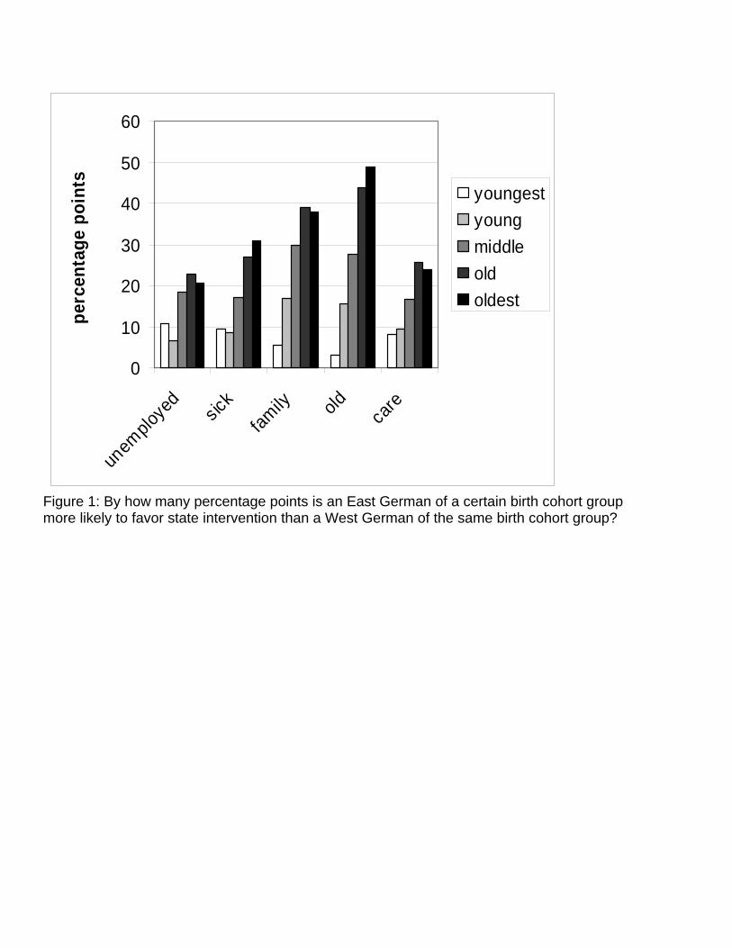
more pro government than the younger in the East, a pattern not observed inthe West in which in fact the older tend to be less pro government than theyounger. Interestingly, for some of the questions the old rather than the oldestgroup in the East shows the maximum support of government. Note that theold ones are the group with the maximum time of the working life spent underCommunism, since they were at least 15 years old at the end of World War II.The quantitative implications of the birth cohort effects are large. Figure 1

represents the results from Table 6 in a different way; it shows by how manypercentage points an East German of a certain cohort group is more likelyto favor state intervention than a West German of the same cohort group.While an East German from the youngest group is only between 3 (column 4)and 11 (column 1) percentage points more likely to be in favor of governmentredistribution than a West German of the same group, an East German bornbefore 1945 is between 21 percentage points (column 1) and 49 percentage points(column 4) more likely than a West German of the same cohortgroup to believein government redistribution.

3.2 Decomposition of change over time

Given that we observe that older East Germans are more in favor of redistri-bution than younger ones, the question arises whether the observed decline inEast Germans’ preferences for redistribution between 1997 and 2002 is simplya result of a shift in the cohort composition, or whether it is caused by chang-ing personal preferences of East Germans. Even if personal preferences wereconstant over time, we would expect that East German preferences convergeon average to West German preferences as older East Germans die and EastGermany becomes populated by relatively younger households who have spentless time of their life under communism.To investigate the relative importance of both effects, in Table 7 we report

results from the baseline regressions in which we include only individuals whoanswer the relevant questions in both 1997 and 2002.18 Hence, all effects ofa change in preferences between 1997 and 2002 are due to changing personalpreferences, and not due to changes in the cohort composition. The interactioneffect between East and year 2002 is still negative in all 5 regressions, andsignificant in all cases except financial security of families (column 3). However,the East time effect is now on average substantially smaller than in the baselineregressions, declining in absolute terms by between 0% (column 1), and 70%(column 3). On average, the East time effect is around 35% smaller than theeffect reported in the baseline results in Table 4. Hence, we conclude thataround 2/3 of the convergence arises from actual convergence of preferences,while around one third arises from changes in the cohort composition.19

18Note that we use an unbalanced sample for the general results.19The number of observation drops by around 22% if we restrict the sample to those indi-

viduals who answer in both 1997 and 2002. Note that the decline in the sample size is notrandom. While in general we use only Eastern households that were added to the survey in1990 and hence should in principle answer the survey in both 1997 and 2002, some members of

10

3.3 The Effect of Communism: Poverty or Preferences?

3.3.1 Individual economic effects

The poor tend to favor government intervention more than the rich. In factin our regressions we always include the logarithmic household income of therespondent as a control, and the coefficient on this variable is always negativeand statistically significant. Hence, we are measuring the effects of having beenin the East controlling for the fact that the respondent’s income might be lowerprecisely because he or she lived in the East. In order to allow for furthernon-linearities between income and preferences, we also include a fourth orderpolynomial of household income instead of the logarithm of household income,and our estimates remain almost unchanged.20

In order to capture the extent to which a household currently benefits fromredistribution, in Table 8 we include as explanatory variable the share of house-hold income that comes from government sources, which we call household gov-ernment transfer ratio.21 One would expect a positive effect of this variableon redistribution; in fact, the coefficient is sometimes positive and significant(column 3), sometimes negative and significant (column 2), and sometimes in-significant. Most importantly, the inclusion of this variable leaves the estimatedEast effects almost unchanged. In addition to current income, expected futureincome may explain preferences for redistribution; individuals who expect torise in the social ladder may oppose redistributive policies which might remainin place for several years22. As a rough measure of the effects of expected futureincome we check whether the growth in income of a respondent between 1997and 2002 effects his/her preferences in 1997. This is a rough test of course,which implies perfect forecasts. The future growth rate of income between 1997and 2002 has a negative effect on preferences in 1997, but again its inclusionleaves the estimates of the East dummy almost unchanged (Table 9).

3.3.2 Aggregate economic effects

In addition to personal income, however, there might be an aggregate incomeeffect; individuals living in regions poorer than average may prefer governmentintervention because of the active redistribution from richer to poorer regions,which in fact takes place in Germany.In Table 10 we include the average per capita income and unemployment

rate of the state of residence, as well as transfers received or paid by the state;note that we continue to include as always the income of the respondent. The

the household might choose not to answer one of the relevant questions in either 1997 and 2002(which should be random), and some members of the households become adults between 1997and 2002, and hence answer the personal questionnaire in 2002, but not in 1997. Therefore,on average the sample should comprise more persons of recent birth cohorts in 2002 than in1997, which makes the convergence effect for East stronger given the estimated cohort effects.20Results are available from the authors upon request.21We calculated this share by adding up personal income from government and non-

government sources respectively over the members of a household.22On this point see Benabou and Ok (2001) and Alesina and La Ferrara (2005).

11

level of per capita income turns out never to have a significant effect. The re-gional unemployment rate has a weak positive influence on preferences for stateintervention; it is only significant in the question regarding the unemployed.Financial transfers have significant positive predictive power for preferences forstate intervention for the unemployed, as well as for people requiring care. Afterincluding these three regional controls, in the regression regarding the unem-ployed the coefficient on the East indicator variable drops from 0.41 to 0.28.This suggests that part of the East effect estimated above had to do with EastGerman states benefitting financially from redistribution. A similar pattern oc-curs with all the other questions. Thus, up to one third of the ”East effect” canbe explained by the fact that the East became poorer during Communism andis now a net beneficiary of redistribution within Germany, rather than to aneffect of Communism on preferences. The respondents’ preferences for publicintervention are influenced by economic effects in the region where they live,but even after controlling for that, we still find a large effect of being from theEast.

3.4 Migration and preferences

So far, we have treated all East Germans as one homogeneous group. Yet, 7percent of East Germans in our sample have migrated to the West. In Table11, we add the dummy variable “East living in East”, which takes on the valueof 1 if an East German lives in the territory of the former East Germany in theobservation year, and 0 otherwise.23

The coefficient on the East-dummy now captures the preferences of an EastGerman living in the West. As the table shows, East Germans living in the Westare more in favor of government intervention than West Germans. However,East Germans living in the East are at least twice as much in favor of governmentintervention than East Germans who moved to the West. This result can beinterpreted in two ways. First, it could be that, having lived among WestGermans for some time, preferences of East Germans who moved to the Westhave converged faster than preferences of East Germans who stayed in the East.Second, those that migrated to the West could be a self-selected group that hadlower preferences for state intervention to begin with. Note e.g. that the averageage of East respondents who moved to the West is 34, while the average age ofEast respondents who stayed in the East is 45.With regard to convergence, one can observe that all the convergence in

preferences between 1997 and 2002 is driven by East Germans who stayed inthe East. The preferences of East Germans who moved to the West do not

23We also estimated a model in which we include instead a dummy variable “East residence”that takes on the value of 1 if the respondent lives in the East in the observation year, regardlessof whether the respondent is from the former East or the former West, as well as interactionsof this variable with the East dummy, the year 2002 dummy, and their interaction (resultsare available from the authors upon request). While this is a better modeling approach, theinterpretation of the results is more complicated. Since only 0.6% of the West Germans inour sample live in the East, we hence decided to refrain from splitting the West Germansaccording to current residence. Results do not change significantly.

12

change in a statistically significant way between 1997 and 2002. Again, thereare several possible explanations for this phenomenon. It could be that pref-erences of East Germans who moved to the West converged initially, but thatthey have reached their new steady-state level by 2002. In this case, we shouldnot expect full convergence either for East Germans staying in the East. Onthe other hand, it could be that those East Germans who moved to the Westnot only had different preferences at the time of migration, but that their pref-erences also exhibit different convergence patterns. In the case of preferencesregarding financial security when unemployed and financial security of families,East Germans who moved to the West even become more pro state over time,although this effect is not statistically significant;24 this might be interpreted asa backlash of preferences after experiencing life in the West.

3.5 Regional differences

In order to gain further insides whether the measured effects really capture theeffect of communism, we analyze regional differences in the effect. We wouldexpect the effect of communism to be relatively homogenous across Easternstates. Hence, we would be worried if the “East” effect on preferences werevery heterogeneous across Eastern states, and especially if it were mostly drivenby one or two single states. Hence, we rerun our baseline regression includingseparate dummies for all 5 Eastern states plus East Berlin instead of one singleEast dummy. Note that, consistent with the East dummy, these dummies referto the state of residence at the time of reunification.As the results in Table 12 show, the coefficients on the Eastern state dummies

are positive and significant in all states. Moreover, they are of similar size acrossthe states. The only slight outlier that emerges is the state of Mecklenburg-Vorpommern, which is in 4 out of 5 cases more pro private forces than theother Eastern states, although it is still relatively pro-government comparedwith West Germany. With regard to convergence, the results are a little bitmore heterogeneous. However, only 5 out of 30 coefficients on the interactionterm between an East German state and the year 2002 turn out not to benegative, while 15 of the 30 coefficients are significantly negative. Every stateshows significant convergence in at least 1 of the 5 questions.We conclude that the effect of Communism on preferences, as well as con-

vergence of preferences over time, can be found in every single East Germanstate, and are not driven by outliers.

4 Social conditions, individual effort and luckWhy do former East Germans favor state intervention? One possibility is thatthey are used to think (partly because of the influence of Communist ideology)that it is “society’s fault” if people are poor, unemployed or in need of help.

24The associated p-values are 0.17 and 0.38.

13

If the individual is not responsible, but society is, then society (i.e. the state)should take care of these problems.In Table 13 we report a regression in which the left hand side is a variable that

takes the value of 1 if the respondent believes that social conditions determineindividual possibilities in life. In column 1, we find a strong effect from beingfrom the East. The probability of believing in the influence of social conditionsis 10 percentage points higher for an East German than a West German. Thecoefficients on individual characteristics seem reasonable. Men believe less insocial conditions than women, unemployed believe more in social conditions,self employed much less etc. In the next column we interact the East indicatorvariable with the age of the respondent and find, once again, a strong ageeffect.25 Older East Germans are more likely to believe in social conditionsas major determinants of individual fortunes than younger East Germans. Weinterpret this as the effect of having lived longer under a Communist regime. Inthe West, the age effect is not significant.Table 14 however shows that the effect of having lived in the East goes well

beyond these beliefs about social conditions. In this table (where as alwayswe control for all individual characteristics), we repeat the baseline regressionincluding the dummy variable capturing beliefs in an important role of socialconditions as control. While the variable capturing the beliefs about socialconditions has a significantly positive influence on preferences for an active staterole, the East indicator variables are still significant and only slightly smallerthan in the baseline results in Table 4. Thus, even after controlling for beliefsregarding social conditions, former East Germans believe in state interventionmore than former West Germans.Alesina and La Ferrara (2005) an Alesina and Glaeser (2004) find that those

who believe that luck determines wealth and success in life are more pro redis-tribution than those who belief that mostly individual effort is responsible forsuccess.26 We pursue this line here as well. Table 15 shows a regression in whichthe left hand side variable is defined as 1 if the respondent believes that luckdetermines individual fortunes. The East indicator variable is now negative. Ifwe put this result together with that of Table 13, it appears that East Germansbelieve more than West Germans that individuals (being their effort or theirluck) matter less than social conditions in determining success or failure in life.Column 2 shows no age effect for East Germans beyond the positive age effectalso observed for West Germans.27 Table 16 shows that those who belief thatluck matters a lot in determining individual success are more favorable to gov-ernment intervention. Not surprisingly, given the lower belief in the role of luckby East Germans, the inclusion of this variable has no significant effect on theeast indicator variable.25As in table 5, we omit higher order terms of age as controls in this regression.26Alesina and Angeletos (2005) and Benabou and Tirole (2004) present models seeking to

explain the equilibrium redsitributive policies as a function of individual beliefs about luckand effort as determinants of success.27Again, we omit higher order terms of age as controls in this regression.

14

5 Final remarksWe find that East Germans belief significantly more so than West Germans thatthe state should be responsible for the financial security of different vulnerablegroups in society, namely the unemployed, the sick, families, the old, and peoplerequiring care. According to our results, it will take about one to two generations(20 to 40 years) for an average East German to have the same views on the roleof the government in society than a West German.The difference in preferences between former East and West Germans is

due in large part to the direct effect of communism. This effect could arisedue to indoctrination, e.g. in public schools, or simply due to becoming usedto an intrusive public sector. A second, indirect effect of communism is thatby making former East Germany poorer than West Germany, it has made theformer more dependent on redistribution and therefore more favorable to it. Theimplication of our findings is that former West Germany has received a major“political shock”, in the sense that the new members of the unified Germanyare much more favorable to state intervention. This shock has potentially long-lasting effects, since we find that preferences need one to two generations toconverge. One caveat to this conclusion, however, is that since we could useonly two survey years, namely 1997 and 2002, we could only estimate a linearconvergence effect. It is possible that the speed of convergence may increaseor decrease. Certainly, even 15 years after reunification former East Germanscontinue to view the role of the state in economic life as much more essentialthan the former West Germans, not exactly a population of libertarians.In evaluating these results, one always has to wonder whether or not these

survey answers are meaningful, namely whether they reflect what individualstruly believe. We are quite confident that they truly reflect preferences fortwo reasons. First, the basic correlations of the answers with variables likeincome, wealth, and labor force status are consistent with obvious individualcost/benefit analyses. Second, evidence on voting behavior in East and Westover the observation period is consistent with the picture emerging from thissurvey. Table A4 shows the share of votes obtained by various parties in thedifferent states in the elections for the federal parliament (Bundestagswahlen)in 1998 and 2002. In this table, the parties are ordered from left to right tocoincide with their position in the political spectrum. Thus, the first columnshows the vote share per state of the most leftist party, the PDS (Partei desDemokratischen Sozialismus), which is in effect the successor party of the SED(Sozialistische Einheitspartei Deutschlands), the ruling party in the GDR. In1998, the percentage of votes received by this party was about 20 per cent inthe East, but only around 1 to 2 per cent in the West; it was around 10 percent in Berlin, which includes both former East and former West Berlin. Thisis consistent with our finding of a much more pro state, left leaning populationin the East, as captured by the survey. Also, comparing the 2002 and 1998elections, we see how the percentage of the PDS votes in the East shrinks sub-stantially, presumably in favor of the SPD, the main center left party, whoseshare increases almost identically to the reduction in votes for the PDS. This

15

indicates a movement away from the communist leaning left toward the centerof the political spectrum, and shows a convergence of the East to the West.This voting behavior is therefore consistent with the preferences regarding stateintervention expressed by the respondents of the survey.

6 References

References[1] Ai, C. and E. C. Norton (2003) "Interaction Terms in Logit and Probit

Models", Economics Letters, Vol. 80, pp. 123-129.

[2] Alesina, A. and G.M. Angeletos (2005): Fairness and Redistribution, Amer-ican Economic Review, forthcoming.

[3] Alesina, A. and E. Glaeser (2004) Fighting Poverty in the U.S. and Europe:A World of Difference, Oxford University Press, Oxford, UK.

[4] Alesina, A. and E. La Ferrara (2005) "Preferences for Redistribution in theLand of Opportunities", Journal of Public Economics (forthcoming).

[5] Benabou, R. and E. Ok (2001): "Social Mobility and the Demand for Re-distribution: The POUM Hypothesis", Quarterly Journal of Economics,116(2), 447-487.

[6] Benabou, R. and J. Tirole (2005): "Belief in a Just World and Redistribu-tive Policies", Princeton University, mimeo.

[7] Corneo, G. (2001) "Inequality and the State: Comparing US and GermanPreferences", Annales d’Economie et de Statistique, 63-64 (2001), 283-296.

[8] Corneo, G. and H.P. Gruner (2002) "Individual Preferences for PoliticalRedistribution" Journal of Public Economics, 83, 83-107.

[9] Fong, C. (2003) “The Tunnel Effect Conjecture, the POUM Hypothesis,and the Behavioral Assumptions of Economics”, mimeo, Carnegie MellonUniversity.

[10] Giavazzi, F. and M. McMahon (2005) "All Talk, No Action: The effects ofreforms that are long discussed but never implemented", mimeo, BocconiUniversity.

[11] Piketty, T. (1995): "Social Mobility and Redistributive Politics", QuarterlyJournal of Economics, 110, 551-584

[12] Ravallion, M. and M. Lokshin (2000), “Who Wants to Redistribute? TheTunnel Effect in 1990 Russia”, Journal of Public Economics, 76, 87-104.

16

[13] Schäfgen, K. (1998): Die Verdoppelung der Ungleichheit. Sozialstrukturund Geschlechterverhältnisse in der Bundesrepublik und in der DDR, Dis-sertation, Humboldt-Universität.

[14] Stephan, H. and E. Wiedemann (1990): Lohnstruktur und Lohndifferen-zierung in der DDR: Ergebnisse der Lohndatenerfassung vom September1988,Mitteilungen aus der Arbeitsmarkt- und Berufsforschung, 23, 550-562.

17

Appendix

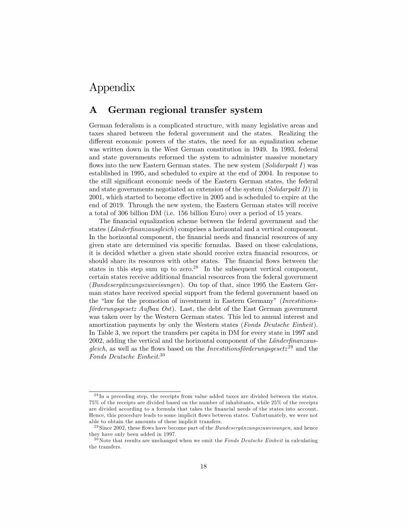
A German regional transfer systemGerman federalism is a complicated structure, with many legislative areas andtaxes shared between the federal government and the states. Realizing thedifferent economic powers of the states, the need for an equalization schemewas written down in the West German constitution in 1949. In 1993, federaland state governments reformed the system to administer massive monetaryflows into the new Eastern German states. The new system (Solidarpakt I ) wasestablished in 1995, and scheduled to expire at the end of 2004. In response tothe still significant economic needs of the Eastern German states, the federaland state governments negotiated an extension of the system (Solidarpakt II ) in2001, which started to become effective in 2005 and is scheduled to expire at theend of 2019. Through the new system, the Eastern German states will receivea total of 306 billion DM (i.e. 156 billion Euro) over a period of 15 years.The financial equalization scheme between the federal government and the

states (Länderfinanzausgleich) comprises a horizontal and a vertical component.In the horizontal component, the financial needs and financial resources of anygiven state are determined via specific formulas. Based on these calculations,it is decided whether a given state should receive extra financial resources, orshould share its resources with other states. The financial flows between thestates in this step sum up to zero.28 In the subsequent vertical component,certain states receive additional financial resources from the federal government(Bundesergänzungszuweisungen). On top of that, since 1995 the Eastern Ger-man states have received special support from the federal government based onthe “law for the promotion of investment in Eastern Germany” (Investitions-förderungsgesetz Aufbau Ost). Last, the debt of the East German governmentwas taken over by the Western German states. This led to annual interest andamortization payments by only the Western states (Fonds Deutsche Einheit).In Table 3, we report the transfers per capita in DM for every state in 1997 and2002, adding the vertical and the horizontal component of the Länderfinanzaus-gleich, as well as the flows based on the Investitionsförderungsgesetz 29 and theFonds Deutsche Einheit.30

28 In a preceding step, the receipts from value added taxes are divided between the states.75% of the receipts are divided based on the number of inhabitants, while 25% of the receiptsare divided according to a formula that takes the financial needs of the states into account.Hence, this procedure leads to some implicit flows between states. Unfortunately, we were notable to obtain the amounts of these implicit transfers.29 Since 2002, these flows have become part of the Bundesergänzungszuweisungen, and hence

they have only been added in 1997.30Note that results are unchanged when we omit the Fonds Deutsche Einheit in calculating

the transfers.

18

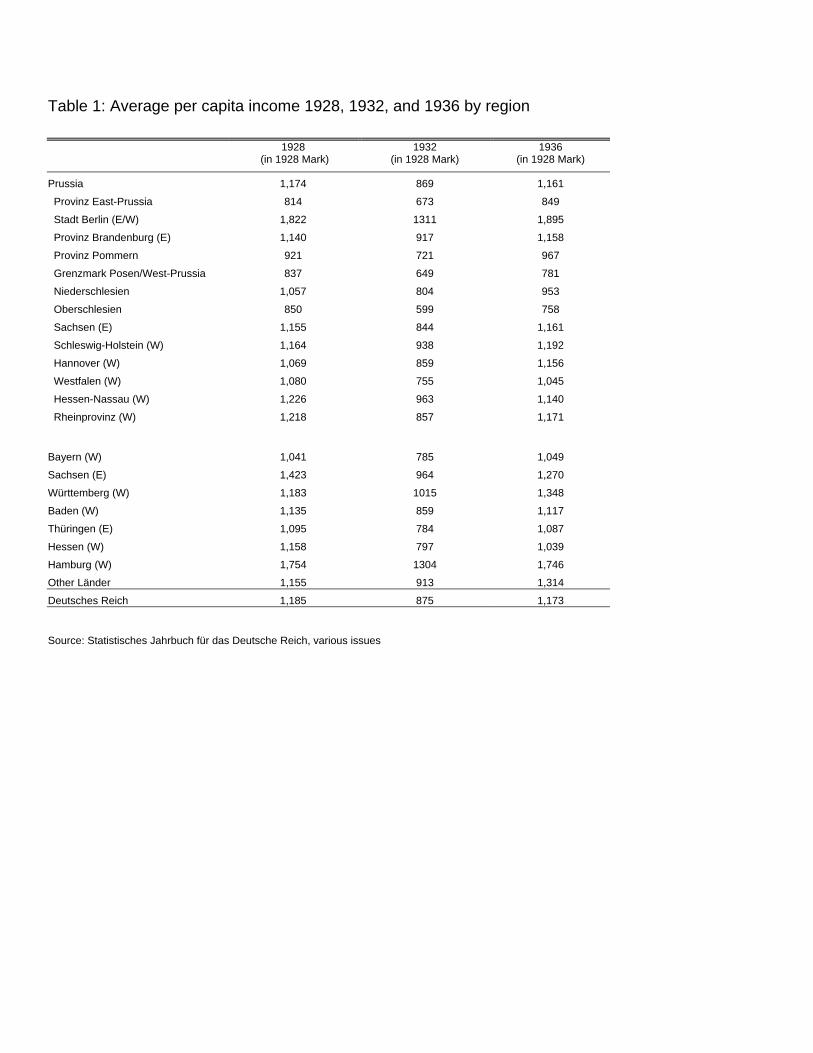
Table 1: Average per capita income 1928, 1932, and 1936 by region

1928 (in 1928 Mark)

1932 (in 1928 Mark)

1936 (in 1928 Mark)

Prussia 1,174 869 1,161

Provinz East-Prussia 814 673 849

Stadt Berlin (E/W) 1,822 1311 1,895

Provinz Brandenburg (E) 1,140 917 1,158

Provinz Pommern 921 721 967

Grenzmark Posen/West-Prussia 837 649 781

Niederschlesien 1,057 804 953

Oberschlesien 850 599 758

Sachsen (E) 1,155 844 1,161

Schleswig-Holstein (W) 1,164 938 1,192

Hannover (W) 1,069 859 1,156

Westfalen (W) 1,080 755 1,045

Hessen-Nassau (W) 1,226 963 1,140

Rheinprovinz (W) 1,218 857 1,171

Bayern (W) 1,041 785 1,049

Sachsen (E) 1,423 964 1,270

Württemberg (W) 1,183 1015 1,348

Baden (W) 1,135 859 1,117

Thüringen (E) 1,095 784 1,087

Hessen (W) 1,158 797 1,039

Hamburg (W) 1,754 1304 1,746

Other Länder 1,155 913 1,314

Deutsches Reich 1,185 875 1,173

Source: Statistisches Jahrbuch für das Deutsche Reich, various issues

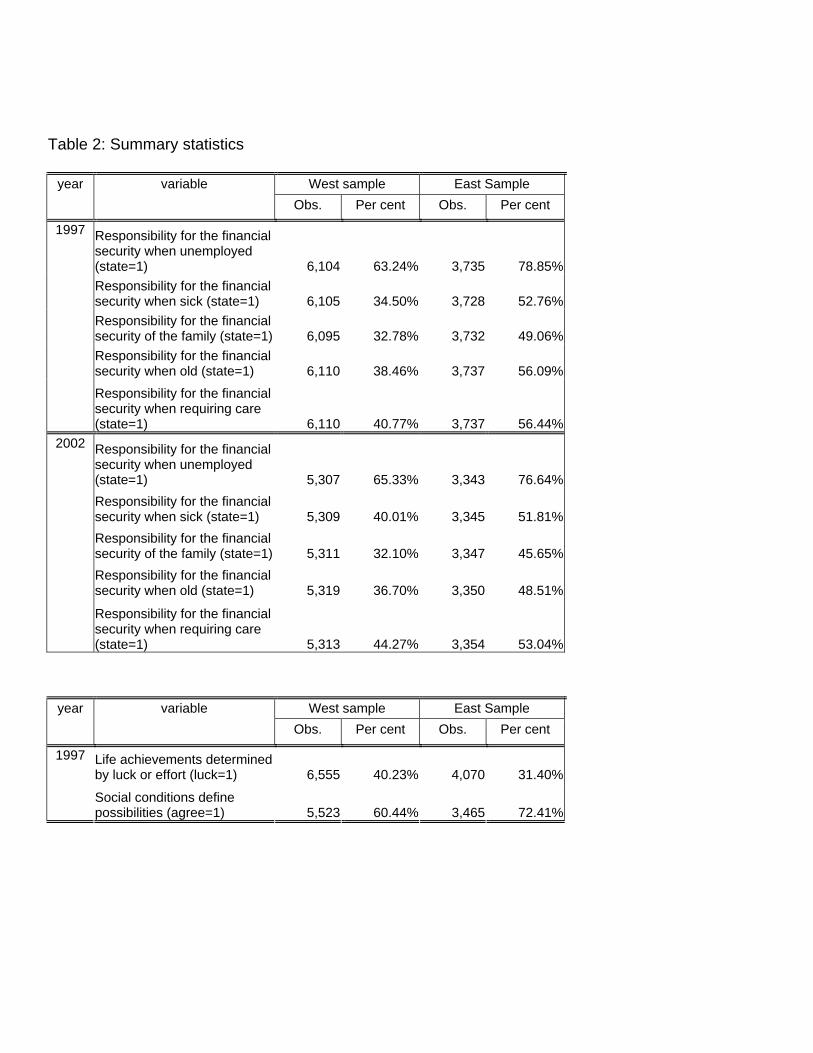
Table 2: Summary statistics

West sample East Sample year variable Obs. Per cent Obs. Per cent

Responsibility for the financial security when unemployed (state=1) 6,104 63.24% 3,735 78.85%Responsibility for the financial security when sick (state=1) 6,105 34.50% 3,728 52.76%Responsibility for the financial security of the family (state=1) 6,095 32.78% 3,732 49.06%Responsibility for the financial security when old (state=1) 6,110 38.46% 3,737 56.09%

1997

Responsibility for the financial security when requiring care (state=1) 6,110 40.77% 3,737 56.44%

Responsibility for the financial security when unemployed (state=1) 5,307 65.33% 3,343 76.64%Responsibility for the financial security when sick (state=1) 5,309 40.01% 3,345 51.81%Responsibility for the financial security of the family (state=1) 5,311 32.10% 3,347 45.65%Responsibility for the financial security when old (state=1) 5,319 36.70% 3,350 48.51%

2002

Responsibility for the financial security when requiring care (state=1) 5,313 44.27% 3,354 53.04%

West sample East Sample year variable Obs. Per cent Obs. Per cent

Life achievements determined by luck or effort (luck=1) 6,555 40.23% 4,070 31.40%

1997

Social conditions define possibilities (agree=1) 5,523 60.44% 3,465 72.41%

Table 3: Average income per capita, unemployment rates, and transfers by states

Average income per capita (in DM)

Unemployment rates (in %)

Transfers per capita (in DM)

1997* 2002 1997 2002 1997* 2002

Berlin 28,830 28,528 17.3 16.9 2,922 3,020 WEST Baden-Württemberg 32,621 34,843 8.7 5.4 -249 -305 Bayern 32,011 33,895 8.7 6.0 -276 -325 Bremen 35,588 37,231 16.8 12.6 3,912 3,458 Hamburg 35,056 36,709 13.0 9.0 -172 -223 Hessen 30,683 32,803 10.4 6.9 -559 -614 Niedersachsen 30,149 31,473 12.9 9.2 285 319 Nordrhein-Westfalen 32,198 34,168 12.2 9.2 -182 -176 Rheinland-Pfalz, Saarland 29,625 31,329 11.0 7.6 720 649 Schleswig-Holstein 31,178 31,655 11.2 8.7 132 278 EAST Brandenburg 26,288 28,047 18.9 17.5 1,889 1,793 Mecklenburg-Vorpommern 24,878 26,834 20.3 18.6 2,067 2,016 Sachsen 25,867 28,099 18.4 17.8 1,912 1,893 Sachsen-Anhalt 25,227 27,313 21.7 19.6 1,998 1,985 Thüringen 25,338 27,941 19.1 15.9 2,015 1,954 * Values adjusted for inflation

Table 4: Basic regression

Responsibility for the financial security when unemployed (state=1)

Responsibility for the financial security when

sick (state=1)

Responsibility for the financial security of the

family (state=1)


old (state=1)

Responsibility for the financial security when requiring care (state=1)

Dependent variable

Coeff. Std. Err. Coeff. Std. Err. Coeff. Std. Err. Coeff. Std. Err. Coeff. Std. Err.

east 0.414 0.029 0.406 0.027 0.405 0.027 0.399 0.027 0.362 0.027

year02 0.068 0.023 0.170 0.023 -0.009 0.024 -0.027 0.023 0.105 0.023

east*year02 -0.124 0.039 -0.163 0.036 -0.063 0.036 -0.146 0.036 -0.177 0.036

age -0.034 0.014 -0.018 0.014 -0.022 0.014 -0.034 0.014 -0.011 0.014

age squared (*103) 0.745 0.283 0.375 0.277 0.473 0.278 0.709 0.273 0.095 0.272

age cubed (*103) -0.005 0.002 -0.002 0.002 -0.003 0.002 -0.004 0.002 -0.0001 0.002

male -0.088 0.022 -0.083 0.021 -0.014 0.022 -0.031 0.022 0.014 0.021

number of children 0.034 0.014 0.035 0.012 0.064 0.012 0.059 0.036 0.109 0.036

number of adults 0.026 0.013 0.049 0.012 0.026 0.011 0.038 0.012 0.011 0.012

married 0.079 0.038 0.109 0.037 0.036 0.036 0.043 0.011 0.008 0.011

divorced 0.095 0.054 0.042 0.052 0.020 0.052 0.063 0.052 0.101 0.050

married but separated 0.028 0.088 -0.008 0.084 -0.031 0.084 0.096 0.084 0.176 0.085

widowed -0.034 0.059 0.053 0.057 -0.020 0.058 -0.005 0.056 0.064 0.056

log(household income) -0.171 0.026 -0.285 0.025 -0.149 0.024 -0.244 0.024 -0.154 0.024

civilservant -0.165 0.056 -0.278 0.058 0.071 0.058 -0.114 0.058 -0.132 0.054

self-employed -0.338 0.052 -0.433 0.052 -0.340 0.052 -0.477 0.052 -0.316 0.051

white-collar worker -0.056 0.032 -0.082 0.030 -0.004 0.031 -0.126 0.030 -0.114 0.030

unemployed 0.153 0.051 -0.008 0.047 0.135 0.047 -0.007 0.046 -0.039 0.046

retired -0.088 0.059 -0.108 0.057 0.137 0.057 -0.001 0.056 0.002 0.056

maternity -0.005 0.079 -0.080 0.077 0.098 0.075 -0.229 0.076 -0.093 0.075

nonworking -0.037 0.043 -0.034 0.042 0.153 0.042 -0.024 0.041 0.016 0.041

training -0.033 0.064 0.003 0.061 -0.079 0.063 -0.056 0.061 -0.004 0.061

other nonworking -0.007 0.051 -0.099 0.049 0.068 0.049 -0.052 0.048 -0.099 0.048

constant 2.165 0.293 2.113 0.283 0.924 0.280 2.143 0.280 1.284 0.276

obs 18,489 18,487 18,485 18,516 18,514

log likelihood -11,070 -12,208 -11,964 -12,265 -12,571

Table 5: Regressions with east*age interaction



sick (state=1)


family (state=1)


old (state=1)


Dependent variable


east 0.029 0.064 -0.035 0.060 -0.032 0.060 -0.225 0.060 0.002 0.059 year02 0.075 0.023 0.178 0.023 -0.001 0.024 -0.016 0.023 0.111 0.023 east*year02 -0.140 0.039 -0.179 0.036 -0.077 0.036 -0.171 0.036 -0.191 0.036 age -0.001 0.001 -0.002 0.001 -0.003 0.001 -0.004 0.001 -0.006 0.001 east*age 0.009 0.001 0.010 0.001 0.010 0.001 0.014 0.001 0.008 0.001 const 1.796 0.213 2.031 0.202 0.818 0.199 1.909 0.200 1.293 0.197 obs 18,489 18,487 18,485 18,516 18,514 log likelihood -11,047 -12,170 -11,928 -12,191 -12,546

Table 6: Regressions with cohorts interacted with east



sick (state=1)


family (state=1)


old (state=1)


Dependent variable


east 0.316 0.068 0.239 0.063 0.141 0.064 0.075 0.064 0.204 0.064 year02 0.069 0.026 0.166 0.026 -0.042 0.027 -0.061 0.026 0.107 0.025 east*year02 -0.114 0.039 -0.141 0.037 -0.037 0.037 -0.112 0.036 -0.159 0.036 young 0.014 0.074 0.015 0.070 -0.210 0.072 -0.218 0.072 -0.030 0.070 middle -0.085 0.100 -0.054 0.095 -0.429 0.097 -0.383 0.096 -0.084 0.094 old -0.067 0.127 -0.104 0.122 -0.492 0.124 -0.518 0.123 -0.098 0.119 oldest -0.022 0.154 -0.117 0.148 -0.431 0.151 -0.484 0.150 -0.019 0.146 young*east -0.118 0.075 -0.008 0.070 0.111 0.071 0.109 0.071 0.002 0.071 middle*east 0.139 0.077 0.145 0.072 0.270 0.073 0.276 0.073 0.136 0.072 old*east 0.329 0.081 0.355 0.075 0.480 0.075 0.603 0.076 0.349 0.075 oldest*east 0.285 0.098 0.431 0.090 0.437 0.090 0.724 0.091 0.379 0.090 const 2.006 0.355 2.220 0.342 0.628 0.341 1.993 0.341 1.204 0.334 obs 18,489 18,487 18,485 18,516 18,514 log likelihood -11,034 -12,172 -11,919 -12,183 -12,538

Table 7: Regressions with individuals who answer in 1997 and 2002



sick (state=1)


family (state=1)


old (state=1)


Dependent variable


east 0.421 0.034 0.373 0.032 0.389 0.032 0.372 0.032 0.322 0.032 year02 0.053 0.026 0.166 0.026 -0.026 0.027 -0.028 0.026 0.098 0.026 east*year02 -0.126 0.043 -0.109 0.040 -0.018 0.040 -0.080 0.040 -0.126 0.040 const 1.946 0.365 2.216 0.356 0.772 0.352 2.222 0.353 1.468 0.348

obs 14,433 14,434 14,471 14,449 14,451 log likelihood -8,623 -9,532 -9,372 -9,555 -9,808 Table 8: Regressions with household government transfer ratio



sick (state=1)


family (state=1)


old (state=1)


Dependent variable


household government transfer ratio 0.031 0.045 -0.071 0.043 0.076 0.042 -0.062 0.043 0.018 0.042 east 0.411 0.030 0.407 0.028 0.403 0.028 0.396 0.028 0.362 0.028 year02 0.064 0.023 0.164 0.023 -0.014 0.024 -0.034 0.024 0.101 0.023 east*year02 -0.117 0.039 -0.162 0.037 -0.068 0.037 -0.143 0.036 -0.179 0.037 const 2.109 0.310 2.254 0.301 0.744 0.297 2.229 0.298 1.219 0.292 obs 17,872 17,871 17,871 17,897 17,895 log likelihood -10,680 -11,806 -11,556 -11,852 -12,156 Table 9: Regressions with future income



sick (state=1)


family (state=1)


old (state=1)


requiring care (state=1)

Dependent variable


future log(income) change 0.008 0.041 -0.127 0.040 -0.038 0.039 -0.071 0.039 -0.066 0.039 east 0.424 0.035 0.371 0.032 0.389 0.032 0.365 0.032 0.322 0.032 const 2.332 0.495 2.669 0.478 0.969 0.479 2.717 0.474 1.945 0.469 obs 7,405 7,403 7,400 7,413 7,412 log likelihood -4,392 -4,817 -4,808 -4,899 -4,993

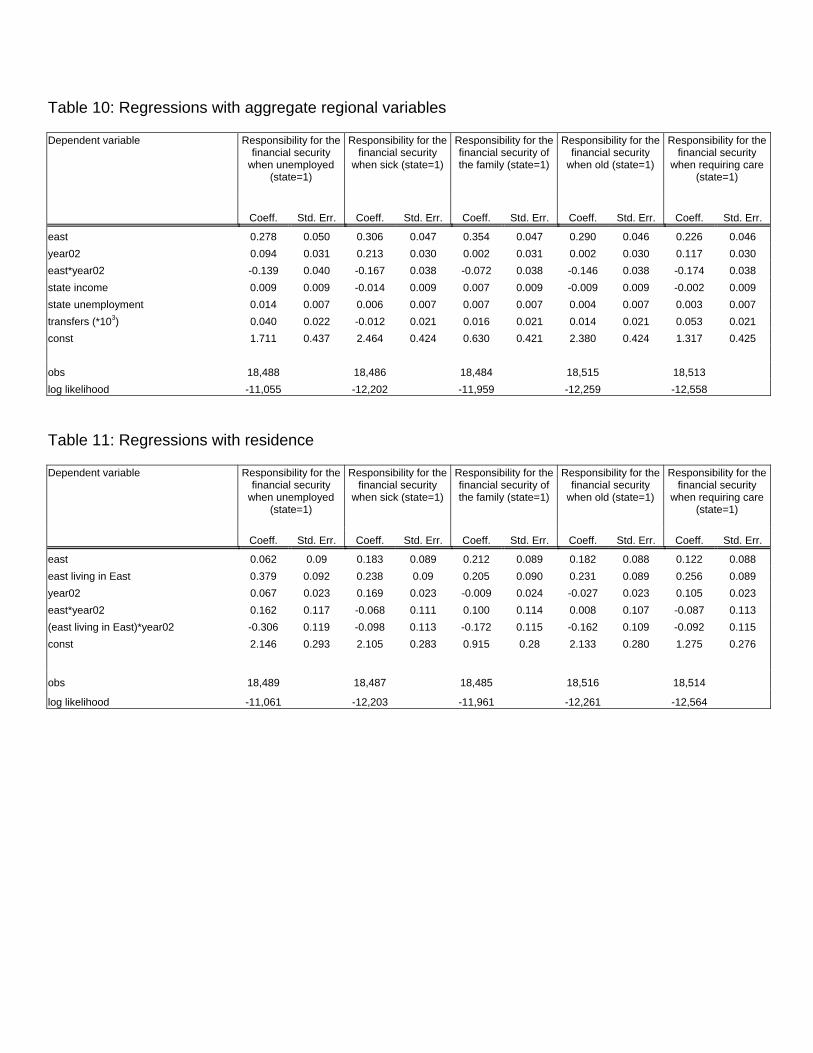
Table 10: Regressions with aggregate regional variables

Responsibility for the financial security

when unemployed (state=1)


when sick (state=1)

Responsibility for the financial security of the family (state=1)


when old (state=1)


when requiring care (state=1)

Dependent variable


east 0.278 0.050 0.306 0.047 0.354 0.047 0.290 0.046 0.226 0.046 year02 0.094 0.031 0.213 0.030 0.002 0.031 0.002 0.030 0.117 0.030 east*year02 -0.139 0.040 -0.167 0.038 -0.072 0.038 -0.146 0.038 -0.174 0.038 state income 0.009 0.009 -0.014 0.009 0.007 0.009 -0.009 0.009 -0.002 0.009 state unemployment 0.014 0.007 0.006 0.007 0.007 0.007 0.004 0.007 0.003 0.007 transfers (*103) 0.040 0.022 -0.012 0.021 0.016 0.021 0.014 0.021 0.053 0.021 const 1.711 0.437 2.464 0.424 0.630 0.421 2.380 0.424 1.317 0.425 obs 18,488 18,486 18,484 18,515 18,513 log likelihood -11,055 -12,202 -11,959 -12,259 -12,558

Table 11: Regressions with residence




when sick (state=1)



when old (state=1)



Dependent variable


east 0.062 0.09 0.183 0.089 0.212 0.089 0.182 0.088 0.122 0.088 east living in East 0.379 0.092 0.238 0.09 0.205 0.090 0.231 0.089 0.256 0.089 year02 0.067 0.023 0.169 0.023 -0.009 0.024 -0.027 0.023 0.105 0.023 east*year02 0.162 0.117 -0.068 0.111 0.100 0.114 0.008 0.107 -0.087 0.113 (east living in East)*year02 -0.306 0.119 -0.098 0.113 -0.172 0.115 -0.162 0.109 -0.092 0.115 const 2.146 0.293 2.105 0.283 0.915 0.28 2.133 0.280 1.275 0.276

obs 18,489 18,487 18,485 18,516 18,514

log likelihood -11,061 -12,203 -11,961 -12,261 -12,564

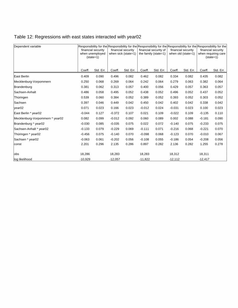
Table 12: Regressions with east states interacted with year02

Responsibility for the

financial security when unemployed

(state=1)


when sick (state=1)



when old (state=1)



Dependent variable


East Berlin 0.409 0.090 0.496 0.082 0.462 0.082 0.334 0.082 0.435 0.082

Mecklenburg-Vorpommern 0.250 0.068 0.269 0.064 0.242 0.064 0.279 0.063 0.382 0.064

Brandenburg 0.381 0.062 0.313 0.057 0.400 0.056 0.429 0.057 0.363 0.057

Sachsen-Anhalt 0.486 0.058 0.495 0.052 0.438 0.052 0.496 0.052 0.437 0.052

Thüringen 0.539 0.060 0.384 0.052 0.389 0.052 0.393 0.052 0.303 0.052

Sachsen 0.397 0.046 0.449 0.042 0.450 0.042 0.402 0.042 0.338 0.042

year02 0.071 0.023 0.166 0.023 -0.012 0.024 -0.031 0.023 0.100 0.023

East Berlin * year02 -0.044 0.127 -0.372 0.107 0.021 0.109 -0.022 0.109 -0.135 0.110

Mecklenburg-Vorpommern * year02 0.082 0.099 -0.012 0.092 0.060 0.089 0.002 0.088 -0.181 0.090

Brandenburg * year02 -0.030 0.085 -0.035 0.075 0.022 0.072 -0.140 0.075 -0.233 0.075

Sachsen-Anhalt * year02 -0.133 0.079 -0.229 0.069 -0.111 0.071 -0.216 0.068 -0.221 0.070

Thüringen * year02 -0.456 0.075 -0.140 0.070 -0.098 0.068 -0.123 0.070 -0.010 0.067

Sachsen * year02 -0.063 0.061 -0.202 0.056 -0.108 0.055 -0.186 0.054 -0.208 0.056 const 2.201 0.296 2.135 0.286 0.897 0.282 2.136 0.282 1.255 0.278

obs 18,286 18,283 18,283 18,312 18,311

log likelihood -10,929 -12,057 -11,822 -12,112 -12,417

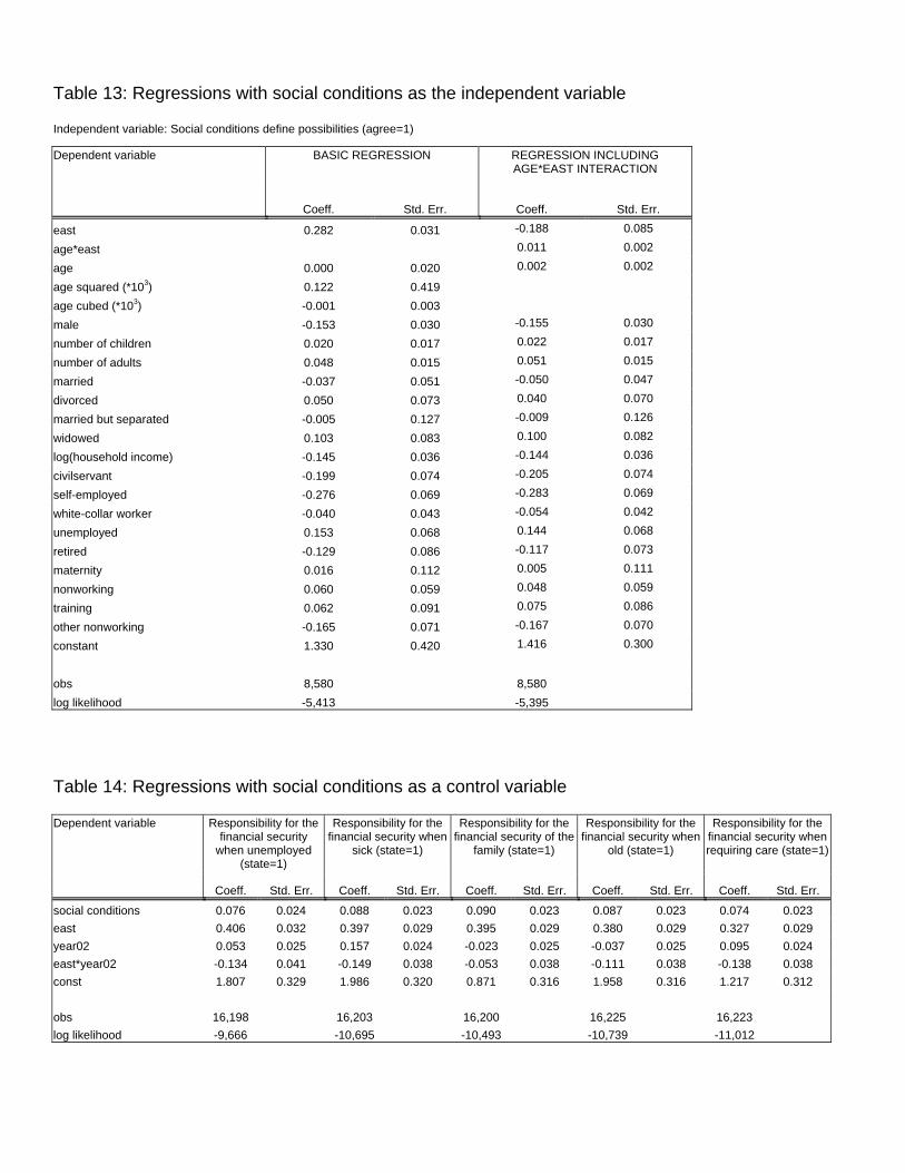
Table 13: Regressions with social conditions as the independent variable

Independent variable: Social conditions define possibilities (agree=1)

BASIC REGRESSION REGRESSION INCLUDING AGE*EAST INTERACTION

Dependent variable

Coeff. Std. Err. Coeff. Std. Err.

east 0.282 0.031 -0.188 0.085

age*east 0.011 0.002

age 0.000 0.020 0.002 0.002

age squared (*103) 0.122 0.419

age cubed (*103) -0.001 0.003

male -0.153 0.030 -0.155 0.030

number of children 0.020 0.017 0.022 0.017

number of adults 0.048 0.015 0.051 0.015

married -0.037 0.051 -0.050 0.047

divorced 0.050 0.073 0.040 0.070

married but separated -0.005 0.127 -0.009 0.126

widowed 0.103 0.083 0.100 0.082

log(household income) -0.145 0.036 -0.144 0.036

civilservant -0.199 0.074 -0.205 0.074

self-employed -0.276 0.069 -0.283 0.069

white-collar worker -0.040 0.043 -0.054 0.042

unemployed 0.153 0.068 0.144 0.068

retired -0.129 0.086 -0.117 0.073

maternity 0.016 0.112 0.005 0.111

nonworking 0.060 0.059 0.048 0.059

training 0.062 0.091 0.075 0.086

other nonworking -0.165 0.071 -0.167 0.070

constant 1.330 0.420 1.416 0.300

obs 8,580 8,580 log likelihood -5,413 -5,395

Table 14: Regressions with social conditions as a control variable




sick (state=1)


family (state=1)


old (state=1)


Dependent variable


social conditions 0.076 0.024 0.088 0.023 0.090 0.023 0.087 0.023 0.074 0.023 east 0.406 0.032 0.397 0.029 0.395 0.029 0.380 0.029 0.327 0.029 year02 0.053 0.025 0.157 0.024 -0.023 0.025 -0.037 0.025 0.095 0.024 east*year02 -0.134 0.041 -0.149 0.038 -0.053 0.038 -0.111 0.038 -0.138 0.038 const 1.807 0.329 1.986 0.320 0.871 0.316 1.958 0.316 1.217 0.312 obs 16,198 16,203 16,200 16,225 16,223 log likelihood -9,666 -10,695 -10,493 -10,739 -11,012

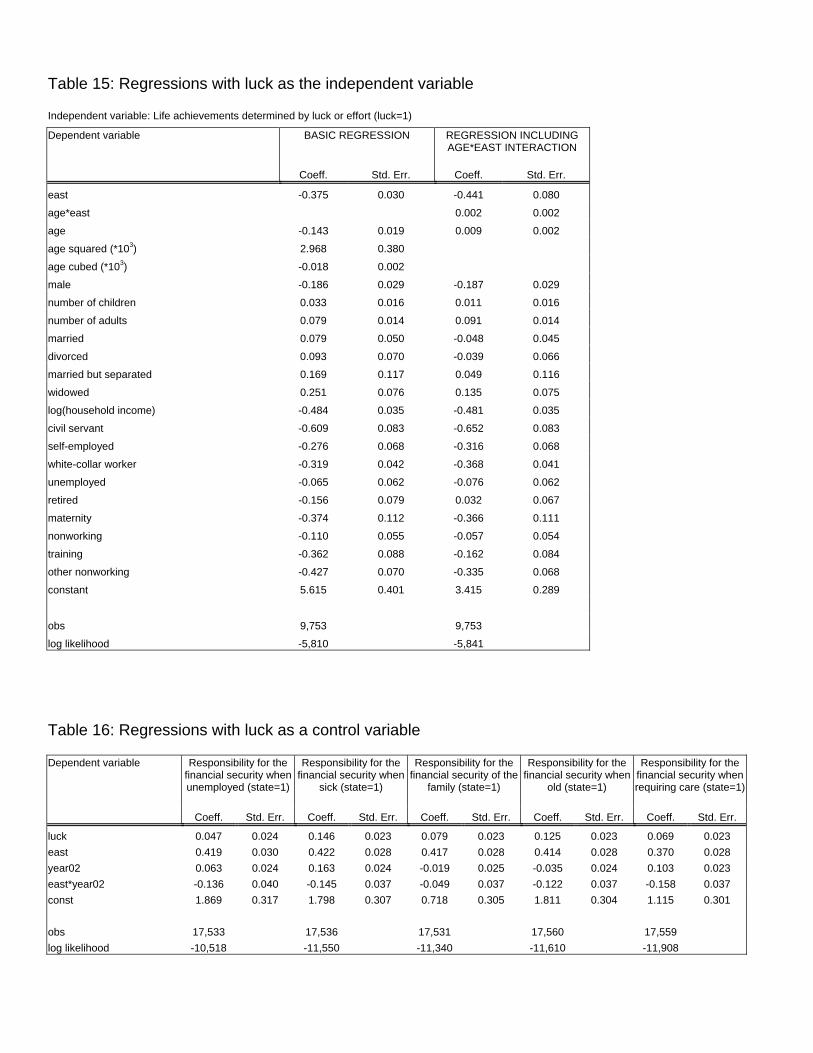
Table 15: Regressions with luck as the independent variable

Independent variable: Life achievements determined by luck or effort (luck=1)

BASIC REGRESSION REGRESSION INCLUDING AGE*EAST INTERACTION

Dependent variable

Coeff. Std. Err. Coeff. Std. Err.

east -0.375 0.030 -0.441 0.080

age*east 0.002 0.002

age -0.143 0.019 0.009 0.002

age squared (*103) 2.968 0.380

age cubed (*103) -0.018 0.002

male -0.186 0.029 -0.187 0.029


number of adults 0.079 0.014 0.091 0.014

married 0.079 0.050 -0.048 0.045

divorced 0.093 0.070 -0.039 0.066

married but separated 0.169 0.117 0.049 0.116

widowed 0.251 0.076 0.135 0.075

log(household income) -0.484 0.035 -0.481 0.035

civil servant -0.609 0.083 -0.652 0.083

self-employed -0.276 0.068 -0.316 0.068

white-collar worker -0.319 0.042 -0.368 0.041

unemployed -0.065 0.062 -0.076 0.062

retired -0.156 0.079 0.032 0.067

maternity -0.374 0.112 -0.366 0.111

nonworking -0.110 0.055 -0.057 0.054

training -0.362 0.088 -0.162 0.084

other nonworking -0.427 0.070 -0.335 0.068

constant 5.615 0.401 3.415 0.289

obs 9,753 9,753

log likelihood -5,810 -5,841

Table 16: Regressions with luck as a control variable



sick (state=1)


family (state=1)


old (state=1)


Dependent variable


luck 0.047 0.024 0.146 0.023 0.079 0.023 0.125 0.023 0.069 0.023 east 0.419 0.030 0.422 0.028 0.417 0.028 0.414 0.028 0.370 0.028 year02 0.063 0.024 0.163 0.024 -0.019 0.025 -0.035 0.024 0.103 0.023 east*year02 -0.136 0.040 -0.145 0.037 -0.049 0.037 -0.122 0.037 -0.158 0.037 const 1.869 0.317 1.798 0.307 0.718 0.305 1.811 0.304 1.115 0.301 obs 17,533 17,536 17,531 17,560 17,559 log likelihood -10,518 -11,550 -11,340 -11,610 -11,908

0

10

20

30

40

50

60

unem

ploye

dsic

kfam

ily old care

perc

enta

ge p

oint

s

youngestyoungmiddleoldoldest

Figure 1: By how many percentage points is an East German of a certain birth cohort group more likely to favor state intervention than a West German of the same birth cohort group?

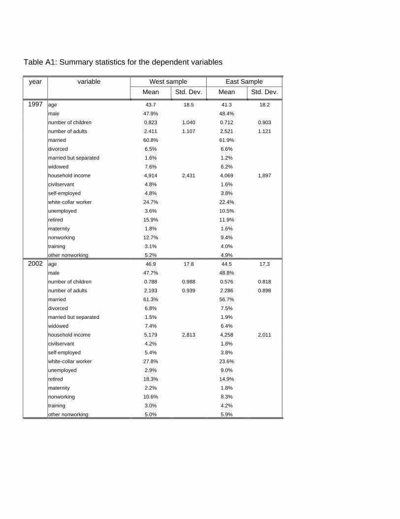
Table A1: Summary statistics for the dependent variables

West sample East Sample year variable Mean Std. Dev. Mean Std. Dev.

age 43.7 18.5 41.3 18.2

male 47.9% 48.4%


number of adults 2.411 1.107 2.521 1.121

married 60.8% 61.9%

divorced 6.5% 6.6%

married but separated 1.6% 1.2%

widowed 7.6% 6.2%

household income 4,914 2,431 4,069 1,897

civilservant 4.8% 1.6%

self-employed 4.8% 3.8%

white-collar worker 24.7% 22.4%

unemployed 3.6% 10.5%

retired 15.9% 11.9%

maternity 1.8% 1.6%

nonworking 12.7% 9.4%

training 3.1% 4.0%

1997

other nonworking 5.2% 4.9%

age 46.9 17.8 44.5 17.3

male 47.7% 48.8%


number of adults 2.193 0.939 2.286 0.898

married 61.3% 56.7%

divorced 6.8% 7.5%

married but separated 1.5% 1.9%

widowed 7.4% 6.4%

household income 5,179 2,813 4,258 2,011

civilservant 4.2% 1.8%

self-employed 5.4% 3.8%

white-collar worker 27.8% 23.6%

unemployed 2.9% 9.0%

retired 18.3% 14.9%

maternity 2.2% 1.8%

nonworking 10.6% 8.3%

training 3.0% 4.2%

2002

other nonworking 5.0% 5.9%

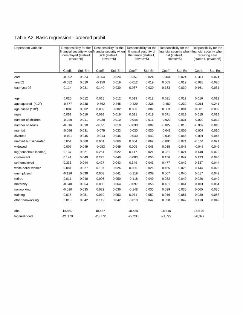
Table A2: Basic regression - ordered probit

Responsibility for the

financial security when unemployed (state=1,

private=5)


sick (state=1, private=5)

Responsibility for the financial security of the family (state=1,

private=5)


old (state=1, private=5)


requiring care (state=1, private=5)

Dependent variable


east -0.392 0.024 -0.364 0.024 -0.357 0.024 -0.344 0.024 -0.314 0.024

year02 -0.032 0.019 -0.150 0.019 -0.012 0.019 0.005 0.019 -0.083 0.020

east*year02 0.114 0.031 0.140 0.030 0.037 0.030 0.133 0.030 0.161 0.031

age 0.026 0.012 0.015 0.012 0.019 0.012 0.021 0.012 0.016 0.012

age squared (*103) -0.577 0.238 -0.362 0.245 -0.429 0.238 -0.480 0.232 -0.261 0.241

age cubed (*103) 0.004 0.002 0.002 0.002 0.003 0.002 0.003 0.001 0.001 0.002

male 0.051 0.019 0.099 0.019 0.021 0.019 0.071 0.019 0.015 0.019

number of children -0.020 0.011 -0.028 0.010 -0.048 0.011 -0.029 0.031 -0.099 0.032

number of adults -0.016 0.010 -0.051 0.010 -0.030 0.009 -0.027 0.010 -0.009 0.010

married -0.056 0.031 -0.079 0.032 -0.030 0.030 -0.041 0.009 -0.007 0.010

divorced -0.101 0.045 -0.013 0.046 -0.040 0.043 -0.035 0.045 -0.091 0.045

married but separated 0.054 0.068 0.001 0.069 0.004 0.067 -0.080 0.071 -0.164 0.071

widowed 0.007 0.049 -0.053 0.049 0.005 0.048 0.035 0.048 -0.048 0.049

log(household income) 0.137 0.021 0.251 0.022 0.147 0.021 0.231 0.021 0.148 0.022

civilservant 0.141 0.049 0.273 0.049 -0.083 0.050 0.156 0.047 0.133 0.046

self-employed 0.333 0.044 0.427 0.043 0.349 0.043 0.477 0.042 0.337 0.044

white-collar worker 0.081 0.027 0.107 0.026 0.035 0.026 0.165 0.026 0.144 0.026

unemployed -0.126 0.039 0.003 0.041 -0.119 0.039 0.007 0.040 0.017 0.042

retired 0.011 0.048 0.095 0.050 -0.118 0.049 0.082 0.049 0.026 0.049

maternity -0.040 0.064 0.035 0.064 -0.097 0.058 0.181 0.061 0.103 0.064

nonworking -0.010 0.035 0.029 0.036 -0.148 0.035 0.039 0.035 0.005 0.035

training 0.016 0.051 0.019 0.053 0.071 0.052 0.016 0.051 0.030 0.053

other nonworking 0.019 0.042 0.112 0.042 -0.019 0.042 0.098 0.042 0.110 0.042

obs 18,489 18,487 18,485 18,516 18,514

log likelihood -21,179 -20,772 -22,233 -21,729 -20,327

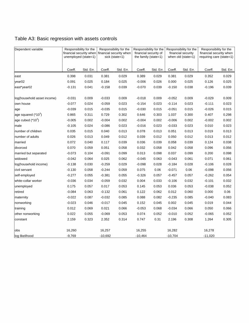
Table A3: Basic regression with assets controls



sick (state=1)



when old (state=1)


Dependent variable


east 0.398 0.031 0.381 0.029 0.389 0.029 0.381 0.029 0.352 0.029

year02 0.091 0.025 0.184 0.025 -0.006 0.026 0.000 0.025 0.126 0.025

east*year02 -0.131 0.041 -0.158 0.039 -0.070 0.039 -0.150 0.038 -0.196 0.039

log(household asset income) -0.031 0.009 -0.033 0.009 -0.018 0.009 -0.052 0.009 -0.029 0.009

own house -0.077 0.024 -0.059 0.023 -0.154 0.023 -0.114 0.023 -0.111 0.023

age -0.039 0.015 -0.035 0.015 -0.030 0.015 -0.051 0.015 -0.026 0.015

age squared (*103) 0.865 0.311 0.729 0.302 0.646 0.303 1.037 0.300 0.407 0.298

age cubed (*103) -0.005 0.002 -0.004 0.002 -0.004 0.002 -0.006 0.002 -0.002 0.002

male -0.105 0.024 -0.086 0.023 -0.016 0.023 -0.033 0.023 0.010 0.023

number of children 0.035 0.015 0.040 0.013 0.078 0.013 0.051 0.013 0.019 0.013

number of adults 0.026 0.013 0.049 0.012 0.039 0.012 0.050 0.012 0.013 0.012

married 0.072 0.040 0.117 0.039 0.036 0.039 0.058 0.039 0.124 0.038

divorced 0.070 0.059 0.051 0.058 0.032 0.058 0.042 0.058 0.096 0.056

married but separated -0.073 0.104 -0.091 0.099 0.013 0.098 0.037 0.099 0.200 0.098

widowed -0.042 0.064 0.025 0.062 -0.045 0.063 -0.043 0.061 0.071 0.061

log(household income) -0.138 0.030 -0.259 0.029 -0.098 0.028 -0.184 0.028 -0.106 0.028

civil servant -0.130 0.058 -0.244 0.059 0.075 0.06 -0.071 0.06 -0.098 0.056

self-employed -0.277 0.055 -0.381 0.055 -0.326 0.057 -0.457 0.057 -0.262 0.054

white-collar worker -0.036 0.034 -0.059 0.032 0.004 0.033 -0.106 0.032 -0.101 0.032

unemployed 0.175 0.057 0.017 0.053 0.145 0.053 0.036 0.053 -0.038 0.052

retired -0.084 0.063 -0.132 0.061 0.122 0.062 0.012 0.060 0.000 0.06

maternity -0.022 0.087 -0.032 0.085 0.088 0.082 -0.235 0.085 -0.040 0.083

nonworking -0.023 0.046 -0.017 0.045 0.152 0.045 0.002 0.045 0.019 0.044

training 0.012 0.069 0.021 0.066 -0.053 0.068 -0.034 0.066 0.050 0.066

other nonworking 0.022 0.055 -0.069 0.053 0.074 0.052 -0.010 0.052 -0.065 0.052

constant 2.159 0.323 2.352 0.314 0.747 0.31 2.196 0.308 1.264 0.305

obs 16,260 16,257 16,255 16,282 16,278

log likelihood -9,769 -10,692 -10,464 -10,704 -11,020

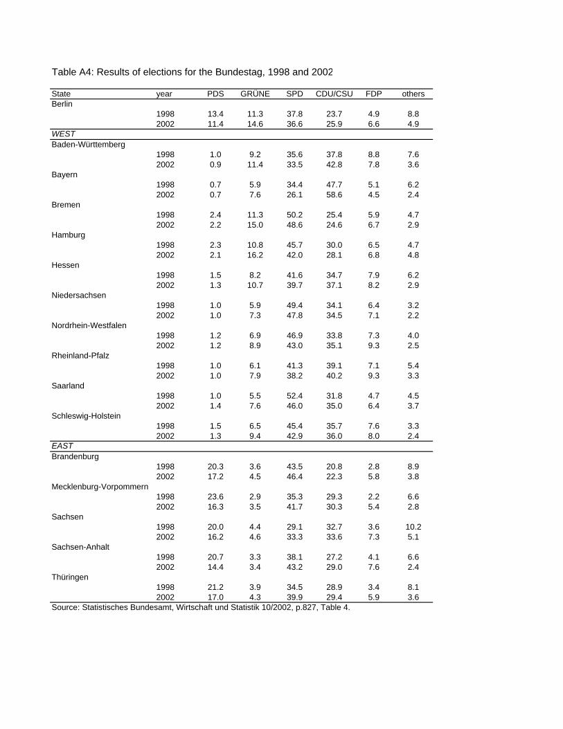
State year PDS GRÜNE SPD CDU/CSU FDP othersBerlin

1998 13.4 11.3 37.8 23.7 4.9 8.82002 11.4 14.6 36.6 25.9 6.6 4.9

WESTBaden-Württemberg

1998 1.0 9.2 35.6 37.8 8.8 7.62002 0.9 11.4 33.5 42.8 7.8 3.6

Bayern1998 0.7 5.9 34.4 47.7 5.1 6.22002 0.7 7.6 26.1 58.6 4.5 2.4

Bremen1998 2.4 11.3 50.2 25.4 5.9 4.72002 2.2 15.0 48.6 24.6 6.7 2.9

Hamburg1998 2.3 10.8 45.7 30.0 6.5 4.72002 2.1 16.2 42.0 28.1 6.8 4.8

Hessen1998 1.5 8.2 41.6 34.7 7.9 6.22002 1.3 10.7 39.7 37.1 8.2 2.9

Niedersachsen1998 1.0 5.9 49.4 34.1 6.4 3.22002 1.0 7.3 47.8 34.5 7.1 2.2

Nordrhein-Westfalen1998 1.2 6.9 46.9 33.8 7.3 4.02002 1.2 8.9 43.0 35.1 9.3 2.5

Rheinland-Pfalz1998 1.0 6.1 41.3 39.1 7.1 5.42002 1.0 7.9 38.2 40.2 9.3 3.3

Saarland1998 1.0 5.5 52.4 31.8 4.7 4.52002 1.4 7.6 46.0 35.0 6.4 3.7

Schleswig-Holstein1998 1.5 6.5 45.4 35.7 7.6 3.32002 1.3 9.4 42.9 36.0 8.0 2.4

EASTBrandenburg

1998 20.3 3.6 43.5 20.8 2.8 8.92002 17.2 4.5 46.4 22.3 5.8 3.8

Mecklenburg-Vorpommern1998 23.6 2.9 35.3 29.3 2.2 6.62002 16.3 3.5 41.7 30.3 5.4 2.8

Sachsen1998 20.0 4.4 29.1 32.7 3.6 10.22002 16.2 4.6 33.3 33.6 7.3 5.1

Sachsen-Anhalt1998 20.7 3.3 38.1 27.2 4.1 6.62002 14.4 3.4 43.2 29.0 7.6 2.4

Thüringen1998 21.2 3.9 34.5 28.9 3.4 8.12002 17.0 4.3 39.9 29.4 5.9 3.6

Source: Statistisches Bundesamt, Wirtschaft und Statistik 10/2002, p.827, Table 4.

Table A4: Results of elections for the Bundestag, 1998 and 2002

Documents

Good-Bye Lenin (Or Not?): The Effect of Communism on