Embed Size (px)
Citation preview

DISCUSSION PAPER SERIES
ABCD
www.cepr.org
Available online at: www.cepr.org/pubs/dps/DP8702.asp www.ssrn.com/xxx/xxx/xxx
No. 8702
GOOD RANKINGS ARE BAD - WHY RELIABLE RANKINGS CAN HURT
CONSUMERS
Laurent Bouton and Georg Kirchsteiger
INDUSTRIAL ORGANIZATION

ISSN 0265-8003
GOOD RANKINGS ARE BAD - WHY RELIABLE RANKINGS CAN HURT CONSUMERS
Laurent Bouton, Boston University Georg Kirchsteiger, ECARES, Université Libre de Bruxelles and CEPR
Discussion Paper No. 8702 December 2011
Centre for Economic Policy Research 77 Bastwick Street, London EC1V 3PZ, UK
Tel: (44 20) 7183 8801, Fax: (44 20) 7183 8820 Email: [email protected], Website: www.cepr.org
This Discussion Paper is issued under the auspices of the Centre’s research programme in INDUSTRIAL ORGANIZATION. Any opinions expressed here are those of the author(s) and not those of the Centre for Economic Policy Research. Research disseminated by CEPR may include views on policy, but the Centre itself takes no institutional policy positions.
The Centre for Economic Policy Research was established in 1983 as an educational charity, to promote independent analysis and public discussion of open economies and the relations among them. It is pluralist and non-partisan, bringing economic research to bear on the analysis of medium- and long-run policy questions.
These Discussion Papers often represent preliminary or incomplete work, circulated to encourage discussion and comment. Citation and use of such a paper should take account of its provisional character.
Copyright: Laurent Bouton and Georg Kirchsteiger

CEPR Discussion Paper No. 8702
December 2011
ABSTRACT
Good rankings are bad - Why reliable rankings can hurt consumers*
Ranking have become increasingly popular on markets for study programs, restaurants, wines, cars, etc. This paper analyses the welfare implication of such rankings. Consumers have to make a choice between two goods of unknown quality with exogenous presence or absence of an informative ranking. We show that existence of the ranking might make all consumers worse off. The existence of a ranking changes the demand structure of consumers. With rigid prices and rationing, the change can be detrimental to consumers due to its effect on rationing. Furthermore, this change in demand can also be detrimental due to consumption externalities. Finally, with perfectly flexible prices the ranking might increase the market power of firms and hence lead to losses for all consumers.
JEL Classification: D1, D4, D6, D8 and L1 Keywords: consumer welfare, externalities, market power, rankings and rationing
Laurent Bouton Department of Economics Boston University 264 Bay State Road Room 548 Boston, MA 02215 USA Email: [email protected] For further Discussion Papers by this author see: www.cepr.org/pubs/new-dps/dplist.asp?authorid=166484
Georg Kirchsteiger ECARES Université Libre de Bruxelles 44 Avenue Jeanne B-1050 Brussels BELGIUM Email: [email protected] For further Discussion Papers by this author see: www.cepr.org/pubs/new-dps/dplist.asp?authorid=132740
* We are grateful to Elena Arias Ortiz, Micael Castanheira, Alessandro Gavazza, Thomas Gall, Alessandro Lizzeri, and Andy Newman for insightful comments. We also benefitted from the comments of the audiences at BU and at the conference on Gaming Incentive Systems in Bonn. All remaining errors are ours. This paper is based on the fourth chapter of Laurent Bouton’s PhD dissertation. It previously circulated under the title “Ranking of Products and Peer Effects: The Market for MBA”.
Submitted 23 November 2011

Good rankings are bad - Why reliable rankings can hurt
consumers∗
Laurent Bouton†and Georg Kirchsteiger‡
First Draft: June 2009§
This Version: October 2011
Abstract
Ranking have become increasingly popular on markets for study programs, restau-
rants, wines, cars, etc. This paper analyses the welfare implication of such rankings.
Consumers have to make a choice between two goods of unknown quality with exogenous
presence or absence of an informative ranking. We show that existence of the ranking
might make all consumers worse off. The existence of a ranking changes the demand
structure of consumers. With rigid prices and rationing, the change can be detrimental
to consumers due to its effect on rationing. Furthermore, this change in demand can
also be detrimental due to consumption externalities. Finally, with perfectly flexible
prices the ranking might increase the market power of firms and hence lead to losses for
all consumers.
1 Introduction
During the last 20 years, rankings have become increasingly popular. While restaurants and
hotels have been ranked for a long time (the first red Michelin guide appeared more than
100 years ago), relatively new rankings cover study programs (see e.g. US News and World
Report’s rankings of colleges and graduate schools, and the FT’s ranking of MBA programs),
wine (e.g. the famous Parker guide), health insurances and health care providers (e.g. The
∗We are grateful to Elena Arias Ortiz, Micael Castanheira, Alessandro Gavazza, Thomas Gall, Alessandro
Lizzeri, and Andy Newman for insightful comments. We also benefitted from the comments of the audiences
at BU and at the conference on Gaming Incentive Systems in Bonn. All remaining errors are ours.†Boston University, Dept. of Economics; E-mail: [email protected].‡ECARES, Université Libre de Bruxelles, ECORE, and CEPR; E-mail: [email protected].§This paper is based on the fourth chapter of Laurent Bouton’s PhD dissertation. It previously circulated
under the title “Ranking of Products and Peer Effects: The Market for MBA”.
1

National Committee for Quality Assurance’s plan ratings). Furthermore, the internet allows
rankings based on consumers evaluation, e.g. in the fields of gastronomy, medical services
(see e.g. Yelp.com), and cars (see e.g. cars.com).
Most of the scientific research on rankings investigates the quality of rankings. In the
context of scientific journals in economics, ranking methods have been discussed e.g. by
Kalaitzidakis et al. (2010), and Palacios-Huerta and Volij (2004). There has been quite some
concern that firms or other interested parties might manipulate the outcome of rankings (see
Dranove et al. 2003 for a case with consumer-input technology; Glazer and McGuire (2006),
and Glazer et al., 2008 for multitasking issues and Sorensen (2006) for effects on products
diversity) and that this might be harmful for (some) consumers. But very little research has
been done on the welfare impact of (correct) rankings (see below for few exceptions). The
literature investigating the quality of rankings seem to be based on the implicit assumption
that better rankings are better - more information should not hurt. If the ranking would
only be used in individual decision problems, better information could indeed never hurt.
However, in many “real-world” markets where rankings play a role agents’ choices are not
adequately described as individual decision problems. Consider study programs: students
learn from their peers, and the network generated at school is crucial for future professional
success. Or consider restaurants: for many customers the value of a dinner is influenced
by the identity of the other customers of the restaurant. Hence, these markets are charac-
terized by consumption externalities. Furthermore, in some market prices are not perfectly
flexible, leading to rationing. A prototypical example are again study programs, where good
programs are typically oversubscribed and hence schools choose among applicants. Finally,
even in markets with fully flexible prices and without externalities rankings might have
negative welfare impacts, if the existence of a ranking increases the market power of the
firms.
To analyze the impact of rankings generated by rationing, externalities, and market
power we use a framework with two types of goods that differ in price and quality. Ex-ante
it is not known whether the expensive good is the good one. We compare the situations
with and without rankings. Since we do not deal with the question of the credibility of
rankings, we assume that the ranking (if it exists) is always informative. Furthermore,
there are two types of consumers, who differ in terms of appreciation for the goods, and in
terms of externalities they inflict on other consumers of the same good. For given prices,
we show that without consumption externalities and capacity constraints, the existence of
a ranking makes all types of consumers weakly better off, and that it can lead to a pareto
improvement. But with externalities or with capacity constraints, the situation is very
2
different. The ranking might lead to an ex-ante pareto deterioration - before the results
of the ranking are known, the expected utility of both types of consumers is strictly lower
with than without the ranking. If the market exhibits capacity constraints and consumer
externalities at the same time, the ranking might even be ex-post detrimental: for all possible
ranking outcomes both types of consumers are worse off with than without the ranking.
These harmful effects are more likely the more random the rationing procedure is and the
more important consumption externalities are.
If one allows for flexible prices and some idiosyncratic preference of each consumer for
one of the goods, the existence of a ranking might hurt the consumers even in markets
without capacity constraints and consumption externalities. Flexible prices do not neces-
sarily overcome the problem of welfare decreasing rankings. To the contrary, they allow for
an additional reason why rankings can hurt consumers. This negative effect is more likely
the more important is the good’s intrinsic quality - about which the ranking informs the
consumers - relative to the consumers’ idiosyncratic preferences for a particular good.
It has been argued that (correct) rankings can hurt some consumers. But our paper is
one of the first showing that rankings can hurt all consumers. Gavazza and Lizzeri (2007)
analyses the impact of rationing on the overall surplus of consumers. In particular, they
show that more information about school quality reduces overall surplus when slots for over-
subscribed schools are distributed randomly. Unlike our paper no form of pareto-efficiency
with respect to the different types of students is considered. Furthermore, this model does
not analyze the impact of consumer’s externalities and flexible prices.1 In the context of
flexible prices, Anderson and Renault (2009) show that better information might decrease
consumer’s surplus. But this results is derived within a matching framework, where the
information refers to horizontal aspects of the good and not to its quality. Morris and Shin
(2002) analyze the impact of public information in a setting in which (i) there is strate-
gic complementary in agents’ actions, and (ii) agents hold private information. They show
that increased precision of public information may be harmful. The reason is that, because
of coordination motivations, agents disregard their private (and more precise) information.
More precise public information might thus lead to more “mistakes” by the agents. Though
driven by the coordination effect of public information, our results are fundamentally differ-
ent. First, agents do not have private information to disregard. Second, public information
has a coordination effect because it reveals that one product is intrinsically better than
the other, not because it indirectly reveals what other agents are going to do. Both in the
rationing and in the consumption externality cases, the coordination effect of public infor-
1 It actually suggests that such a negative effect does not hold when prices are flexible.
3

mation leads to collateral damages that exists because of the strategic complementaries in
consumers’ actions.
The rest of the paper is organized as follows. Section 2 lays out the setup. Section 3
analyzes the effects of rankings under the assumption that prices are given and equal to the
marginal costs. It identifies two features of market that may make rankings undesirable:
capacity constraints and consumption externalities. Section 4 relaxes the assumption of
given prices and analyzes the effects of rankings under price flexibility. It shows that rankings
may affect firms market power through an increase in products differentiation. Ratings thus
affect prices and may ultimately diminish consumers welfare. Section 5 concludes.
2 Setup
We consider a market where each consumer acquires one unit of a good. There are two
goods available, and the quality of each good is unknown. If the ranking exists, it provides
additional information about the qualities. Consumption of a particular good may lead to
externalities for the other consumers of the same brand. Capacity constraints may prevent
one firm to fully satisfy the demand.
Goods. Each consumer acquires one unit of one good. There are two goods2, m ∈M =
{e, c}. Both goods are produced by a constant returns to scale technology, with gm denotingthe unit costs of production of good m. We assume that good e has higher production costs,
i.e. ge > gc. The price for good m is denoted by fm. In Section 3 we will analyze the case
were prices are fixed with fe > fc, whereas in section in Section 4 we study the effects of
rankings when firms compete in prices.
One of the two goods is of high intrinsic quality, the other one of low quality. With a
commonly known ex-ante probability λ0 > 0.5 good e has the higher quality. The quality
is measured such that it is proportional to the direct utility gained from consuming the
respective good, without taking the (potential) externality into account.
Ranking. If a ranking exists, it is published before the consumers decide which good
to request. It (partially) resolves the uncertainty about the intrinsic quality of the good.3
More precisely, with the commonly known probability α ∈ (0.5, 1] the ranking reflects thetrue qualities. In case that good e is rated higher than good c, Bayesian updating implies
2The two goods should be viewed as close substitutes, e.g. dinner in two different restaurants, study
programs in the same field at two different universities, etc.3 In a previous version of the paper we allowed the ranking to also reflects the externalities. All of the
main results could be derived with such a formulation, but this analysis is considerably more complicated.
4

that the probability of good e being the good one is
λ1 =αλ0
αλ0 + (1− α)(1− λ0)> λ0. (1)
In case the ranking ranks good c higher, the probability of good e being the good one is
λ2 =(1− α)λ0
(1− α)λ0 + α(1− λ0)< λ0. (2)
We will not consider the exceptional case where α is such that λ2 = 12 .We use the superscript
ρ ∈ {0, 1, 2} to identify the three different situations with respect to the ranking. A valueof ρ = 0 refers to a situation without ranking, a value of ρ = 1 to a situation in which
the ranking ranks good e higher (called confirmative ranking), and a value of ρ = 2 to a
situation in which the ranking ranks good c higher (called surprise ranking).
Consumers. There is a continuum [0, 2] of consumers. There are two types of con-
sumers, t ∈ T = {1, 2} with type 1 providing the “better” externalities if any (the exactmeaning of the types will be defined below). The consumers’ population is composed of
equal fractions of these two types.
Strategies. All consumers decide simultaneously which good they request to buy. The
set of pure strategies of consumer i is given by:
si ∈ {e, c}
where si = m means that consumer i wants to buy good m. We denote by x1 (x2) the
fraction of type 1 (2) consumers wanting to buy good e.
Capacity constraints and selection process. For simplicity we assume that the
supply of each good is the same and denoted by z.4 To make sure that the whole market
can be served, z is larger than 1. If z ≥ 2 then the whole market can be served just by onegood - there are no capacity constraints. If z < 2, the provider of a particular good has
to select among their potential consumers whenever all the consumers want the same good.
We assume that those consumers who do not get their preferred good are willing to buy
the other good - it is always better to consume any of the two goods than none of them.
Formally, we denote by nt(x1, x2) the mass of consumers of type t who get good e when x1
type 1 and x2 type 2 consumer want good e. This function is assumed to be continuous.
For simplification, we assume that both types of producers use the same selection process.
This implies that nt(x1, x2) = 1− nt(1− x1, 1− x2).
4Allowing for different supplies would considerably complicate the notation without changing any of our
results.
5

The probability of an agent to get a particular good depends on his type, on his strategy,
and on the strategy distribution of the whole population. Denote by pmt (si, x1, x2) the
probability of an agent of type t to get good m when his strategy is si and (x1, x2) is
the strategy distribution of the whole population. Since the whole market can be served
by both goods together and each agent gets one good, pmt (si, x1, x2) = 1 − pm0
t (si, x1, x2)
for m 6= m0. Hence, we simplify notation by pet (si, x1, x2) = pt(si, x1, x2). In order to
further characterize nt(x1, x2) and pt(si, x1, x2) we have to distinguish between three cases:
x1 + x2 > z, z ≥ x1 + x2 ≥ 2− x1 − x2, and x1 + x2 < 2− x1 − x2.
If x1 + x2 > z, there is excess demand for good e. Since the good is sold up to the
capacity constraint, it holds that n1(x1, x2) = z − n2(x1, x2). The providers may want to
select for one type of consumers, but we assume that this selection process is not perfect.
So even if the providers would prefer only consumers of one type, they cannot detect all of
them. This implies that x1 > n1 > 0, x2 > n2 > 0. If x1 strictly increases (for given x2), n1
strictly increases and n2 strictly decreases. If x2 strictly increases (for given x1), n1 strictly
decreases and n2 strictly increases. The probabilities of getting the goods are given by:
p1(e, x1, x2) =n1(x1, x2)
x1; p2(e, x1, x2) =
z − n1(x1, x2)
x2;
p1(c, x1, x2) = p2(c, x1, x2) = 0.
If z ≥ x1 + x2 ≥ 2− x1 − x2, there is no excess demand for any of the goods, and each
consumer gets the good he wants. This implies that n1(x1, x2) = x1 and n2(x1, x2) = x2.
Furthermore
p1(e, x1, x2) = p2(e, x1, x2) = 1,
p1(c, x1, x2) = p2(c, x1, x2) = 0.
If x1 + x2 < 2 − x1 − x2, there is excess demand for good c, and 1 − n1(x1, x2) =
z − (1 − n2(x1, x2)). Since the selection process is the same for both types of producers,
1− nt(x1, x2) = nt(1− x1, 1− x2). The mass of consumers of type 1 who consume good c,
1−n1(x1, x2), strictly increases in the number of type-1 applications for c, 1−x1, and strictlydecreases in the number of type 2 applications for c, 1 − x2. The acceptance probabilities
are given by
p1(e, x1, x2) = p2(e, x1, x2) = 1,
p1(c, x1, x2) = 1− n1(1− x1, 1− x2)
1− x1; p2(c, x1, x2) = 1−
n2(1− x1, 1− x2)
1− x1.
Note that for all three cases, n1(x1, x2) strictly increases in x1 and weakly decreases in
x2. Conversely, n2(x1, x2) strictly increases in x2 and weakly decreases in x1. Furthermore,
6

pt(e, x1, x2) > pt(c, x1, x2) - the probability of getting a good is higher when one applies for
it than when one does not.
Externalities. Consumption may lead to (positive or negative) externalities. Type 1
consumers create better (i.e. either more positive or less negative) externalities than type
2 consumers. Denote by qm(n1, n2) the externality experienced by a consumers of good
m when n1 (n2) type 1 (2) consumers consume good e. The externalities are assumed to
increase in the number of type 1 and to decrease in the number of type 2 consumers of
the good. To simplify we assume that the externalities depend only on the composition of
actual consumers and not on the good of the good, i.e. qe(n1, n2) = qc(1− n1, 1− n2). Let
q(x1, x2) = qe(n1(x1, x2), n2(x1, x2)) − qc(n1(x1, x2), n2(x1, x2)). Since the number of type
1 (2) consumers of good e strictly increases in x1 (x2) and weakly decreases in x2 (x1), it
holds that q(x1, x2) strictly increases in x1 and strictly decreases in x2. For the case without
externalities, we have qe(n1, n2) = 0.
Utility. Denote by bht (blt) the evaluation by a type t consumer of the intrinsic quality
of a good when this quality is high (low), with bht > blt. The expected utility of applying
for good si depends on whether the consumer actually gets the good e or c, whether this
good is of high/low intrinsic quality, on how the consumer values this intrinsic quality, and
on the externalities (i.e. the behavior of other consumers). Formally
uρt (si, xρ1, x
ρ2) =
pt(si, xρ1, x
ρ2)³−fe + λρbht + (1− λρ)blt + qe(n1(x1, x2), n2(x1, x2))
´+ (3)
(1− pt(si, xρ1, x
ρ2))³−f c + (1− λρ)bht + λρblt + qc(n1(x1, x2), n2(x1, x2))
´.
3 Capacity Constraints and Externalities
In this section, we study the case where prices are fixed, with good e being more expensive
than good c (i.e. fe > f c). With fixed prices, we show that rankings are always welfare
improving provided that there are no capacity constraints or consumption externalities. But
the presence of capacity constraints or consumption externalities rankings can lead to an
ex-ante Pareto deterioration. And with a combination of both capacity constraints and
consumption externalities the rankings might be Pareto-dominated even from an ex-post
viewpoint.
7

3.1 Equilibrium Analysis
We characterize the set of equilibria for generic parameter values (i.e. we exclude the case
in which bh1 − bl1 = bh2 − bl2) when prices are given.
Since pt(e, x1, x2) > pt(c, x1, x2) it holds that ut(e, x1, x2) ≥ ut(c, x1, x2) whenever
−fe + λbht + (1− λ)blt + qe(n1(x1, x2), n2(x1, x2)) (4)
≥ −f c + (1− λ)bht + λblt + qc(n1(x1, x2), n2(x1, x2)).
Letting f = fe − f c > 0 and bt = bht − blt > 0, and q(x1, x2) = qe(n1(x1, x2), n2(x1, x2)) −qc(n1(x1, x2), n2(x1, x2)), the equilibrium condition becomes:
bt(2λ− 1) + q(x1, x2)− f ≥ 0, (5)
The following Lemma follows directly from condition (5).
Lemma 1 The Nash equilibria of the games with and without ranking, xρ∗ = (x1∗1 , x1∗2 , x2∗1 , x2∗2 )
and x0∗ = (x0∗1 , x0∗2 ), fulfill the following conditions:
(i) xρ∗1 = 0⇒ −f + b1(2λρ − 1) + q(xρ∗1 , xρ∗2 ) ≤ 0,
(ii) xρ∗1 ∈ (0, 1)⇒ −f + b1(2λρ − 1) + q(xρ∗1 , xρ∗2 ) = 0,
(iii) xρ∗1 = 1⇒ −f + b1(2λρ − 1) + q(xρ∗1 , xρ∗2 ) ≥ 0,
(iv) xρ∗2 = 0⇒ −f + b2(2λρ − 1) + q(xρ∗1 , xρ∗2 ) ≤ 0,
(v) xρ∗2 ∈ (0, 1)⇒ −f + b2(2λρ − 1) + q(xρ∗1 , xρ∗2 ) = 0,
(vi) xρ∗2 = 1⇒ −f + b2(2λρ − 1) + q(xρ∗1 , xρ∗2 ) ≥ 0,
for any ρ ∈ {0, 1, 2}.
Combining this result with condition (5), we obtain the following Lemma:
Lemma 2 For any ρ ∈ {0, 1, 2}, we have that:i) If b1(2λρ − 1) > b2(2λ
ρ − 1), then xρ∗2 > 0 implies xρ∗1 = 1.
ii) If b1(2λρ − 1) < b2(2λρ − 1), then xρ∗2 < 1 implies xρ∗1 = 0.
Using this Lemma, we can characterize the set of equilibria for generic parameter values:
Proposition 1 The equilibria of the game with and without rankings, i.e. xρ∗ and x0∗, are
fully characterized by the following conditions for generic parameter values:
1. Whenever b1(2λρ − 1) > b2(2λρ − 1):
(a) If b2(2λρ − 1) + q(1, 1) > f, then xρ∗1 = xρ∗2 = 1;
8

(b) If b2(2λρ − 1) + q(1, 0) > f and b2(2λρ − 1) + q(1, 1) < f, then xρ∗1 = 1 and
x∗2 ∈ (0, 1) solves b2(2λρ − 1) + q(1, xρ∗2 ) = f ;
(c) If b1(2λρ − 1) + q(1, 0) > f and b2(2λρ − 1) + q(1, 0) < f, then xρ∗1 = 1 and
xρ∗2 = 0;
(d) If b1(2λρ − 1) + q(1, 0) > f and b1(2λρ − 1) + q(0, 0) < f, then xρ∗2 = 0 and
x∗1 ∈ (0, 1) solves b1(2λρ − 1) + q(xρ∗1 , 0) = f ;
(e) If b1(2λρ − 1) + q(0, 0) < f, then xρ∗1 = xρ∗2 = 0.
2. Whenever b1(2λρ − 1) < b2(2λρ − 1):
(a) If b1(2λρ − 1) + q(1, 1) > f, xρ∗1 = xρ∗2 = 1;
(b) If b1(2λρ − 1) + q(0, 1) < f and b1(2λρ − 1) + q(1, 1) > f, then xρ∗2 = 1 and
x∗1 ∈ (0, 1) solves b1(2λρ − 1) + q(xρ∗1 , 1) = f ;
(c) If b1(2λρ − 1) + q(0, 1) < f and b2(2λρ − 1) + q(0, 1) > f, then xρ∗1 = 0 and
xρ∗2 = 1;
(d) If b2(2λρ − 1) + q(0, 1) > f and b2(2λρ − 1) + q(0, 0) < f, then xρ∗1 = 0 and
x∗2 ∈ (0, 1) solves b2(2λρ − 1) + q(0, xρ∗2 ) = f ;
(e) If b1(2λρ − 1) + q(0, 0) < f, then xρ∗1 = xρ∗2 = 0.
Proof: see Appendix
It can be easily checked that Proposition 1 guarantees the existence of pure strategy
equilibria. Furthermore, without externalities, i.e. if q is a constant, for generic parameter
values the equilibrium of each of the games is unique and symmetric, i.e. all consumers of
the same type request the same good.
3.2 Welfare analysis
For the welfare analysis, we will not take into account which of the individual agents con-
sumes which good, since this is generally also determined by the random selection process.
Rather, the welfare analysis will investigate the allocation of goods between the two types,
i.e. n1 and n2, and the resulting average payoff of an agent of a particular type. Denote by
n0 = (n01, n02), n
1 = (n11, n12), n
2 = (n21, n22) the allocations without ranking, with confirma-
tive ranking (e is ranked better than c), and with surprise ranking (c ranked higher than
e) respectively. Since the population of each type is 1, nρt denotes also the probability that
a consumer of type t consumes good e for ρ = 0, 1, 2. The expected payoffs without, with
9

confirmative, and with surprise ranking are given by:
U0t (n0) = λ0[n0t
³−fe + bht + qe(n01, n
02)´+ (1− n0t )
³−f c + blt + qc(n01, n
02)´] +¡
1− λ0¢[n0t
³−fe + blt + qe(n01, n
02)´+ (1− n0t )
³−f c + bht + qc(n01, n
02)´] (6)
U1t (n1) = λ1
hn1t
³−fe + bht + qe(n11, n
12)´+ (1− n1t )
³−fc + blt + qc(n11, n
12)´i+
+(1− λ1)hn1t
³−fe + blt + qe(n11, n
12)´+ (1− n1t )
³−f c + bht + qc(n11, n
12)´i(7)
U2t (n2) = λ2
hn2t
³−fe + bht + qe(n21, n
22)´+ (1− n2t )
³−fc + blt + qc(n21, n
22)´i+
+(1− λ2)hn2t
³−fe + blt + qe(n21, n
22)´+ (1− n2t )
³−f c + bht + qc(n21, n
22)´i
.(8)
Using these expected payoffs and taking into account the possible multiplicity of equi-
libria we introduce the following efficiency notion (remember that α is the probability that
the ranking reflects the true qualities):
Definition 1 The presence of the ranking ex-ante dominates its absence if for all equilib-
rium values of n0, n1, and n2 and for both t the following holds:£λ0α+ (1− λ0)(1− α)
¤U1t (n
1, n2) +£(1− α)λ0 + α(1− λ0)
¤U2t (n
1, n2) ≥ U0t (n0), (9)
with strict inequality for one of these inequalities.
The absence of the ranking ex-ante dominates its presence when the opposite holds.
Using this efficiency notion, we get the following proposition:
Proposition 2 Without consumption externalities and without capacity constraint, for any
equilibrium x∗t = (x0∗t , x1∗t , x2∗t ) for generic values of blt, b
ht , f
e, fc, λ0, and α and for t ∈{1, 2}:(i) Condition (9) is satisfied (with strict inequality whenever x0∗t 6= x1∗t or x0∗t 6= x2∗t ).
(ii) There is an open set of parameter values such that the ranking ex-ante dominates its
absence.
Proof. See Appendix
Without capacity constraints and without externalities, the “game” is actually an in-
dividual decision problem without strategic interaction. Therefore, better information can
never hurt.
This result does not hold any longer in the presence of the capacity constraints, as the
following proposition shows:
10
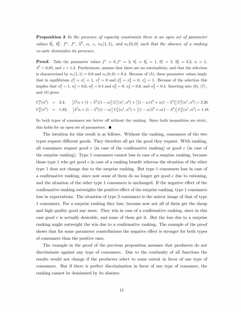
Proposition 3 In the presence of capacity constraints there is an open set of parameter
values blt, bht , f
e, f c, λ0, α, z, n1(1, 1), and n1(0, 0) such that the absence of a ranking
ex-ante dominates its presence.
Proof. Take the parameter values fc = 0, fe = 2, bl1 = bl2 = 1, bh1 = 5, bh2 = 3.2, α = 1,
λ0 = 0.85, and z = 1.2. Furthermore, assume that there are no externalities, and that the selection
is characterized by n1(1, 1) = 0.6 and n1(0, 0) = 0.4. Because of (5), these parameter values imply
that in equilibrium x01 = x11 = 1, x21 = 0 and x02 = x22 = 0, x12 = 1. Because of the selection this
implies that n01 = 1, n11 = 0.6, n
21 = 0.4 and n02 = 0, n
12 = 0.6, and n22 = 0.4. Inserting into (6), (7) ,
and (8) gives:
U01 (n0) = 2.4;
£λ0α+ (1− λ0)(1− α)
¤U11 (n
1, n2) +£(1− α)λ0 + α(1− λ0)
¤U21 (n
1, n2) = 2.26
U02 (n0) = 1.33;
£λ0α+ (1− λ0)(1− α)
¤U12 (n
1, n2) +£(1− α)λ0 + α(1− λ0)
¤U22 (n
1, n2) = 1.18.
So both types of consumers are better off without the ranking. Since both inequalities are strict,
this holds for an open set of parameters.
The intuition for this result is as follows. Without the ranking, consumers of the two
types request different goods. They therefore all get the good they request. With ranking,
all consumers request good e (in case of the confirmative ranking) or good c (in case of
the surprise ranking). Type 1 consumers cannot lose in case of a surprise ranking, because
those type 1 who get good c in case of a ranking benefit whereas the situation of the other
type 1 does not change due to the surprise ranking. But type 1 consumers lose in case of
a confirmative ranking, since now some of them do no longer get good e due to rationing,
and the situation of the other type 1 consumers is unchanged. If the negative effect of the
confirmative ranking outweights the positive effect of the surprise ranking, type 1 consumers
lose in expectations. The situation of type 2 consumers is the mirror image of that of type
1 consumers. For a surprise ranking they lose, because now not all of them get the cheap
and high quality good any more. They win in case of a confirmative ranking, since in this
case good e is actually desirable, and some of them get it. But the loss due to a surprise
ranking might outweight the win due to a confirmative ranking. The example of the proof
shows that for some parameter constellations the negative effect is stronger for both types
of consumers than the positive ones.
The example in the proof of the previous proposition assumes that producers do not
discriminate against any type of consumers. Due to the continuity of all functions the
results would not change if the producers select to some extent in favor of one type of
consumers. But if there is perfect discrimination in favor of one type of consumer, the
ranking cannot be dominated by its absence.
11

Proposition 4 For generic values of blt, bht , f
e, f c, λ0 and α the absence of the ranking
does not ex-ante dominate its presence when all the producers do discriminate perfectly in
favor of one type of consumers.
Proof. Let t be the type of consumer for which it is discriminated for. This implies every consumer
of type t gets the good he wants, i.e. nρt = xρt . Therefore, the proof of proposition 2 holds for type
t.
We have seen an example where both types of consumers are strictly better off without
the ranking in the presence of capacity constraints and without perfect discrimination.
Without capacity constraints, but with externalities one can get the same result.
Proposition 5 With externalities there is an open set of parameter values blt, bht , f
e, f c,
λ0, α,qe(1, 0), qe(1, 1),qe(0, 0), qc(1, 0), qc(1, 1), qc(0, 0) such that the absence of a ranking
ex-ante dominates its presence.
Proof. Assume that there are no capacity constraints, and take the parameter values fc = 0, fe =0.35, bl1 = bl2 = 1, b
h1 = 1.54, b
h2 = 1.3, α = 1, λ
0 = 0.9, qe(1, 0) = qc(0, 1) = 0.8, qe(1, 1) = qc(0, 0) =
0.71, qe(0, 0) = qc(1, 1) = 0.65, and qe(0, 1) = qc(1, 0) = 0.7. Because of (5), these parameter values
imply that the unique equilibrium is such that: x01 = x11 = 1, x21 = 0 and x02 = x22 = 0, x
12 = 1.
Because there is no capacity constraint, nρt = xρt ∀t, ρ. Inserting into (6), (7) , and (8) gives:
U01 (n0) = 1.936;
£λ0α+ (1− λ0)(1− α)
¤U1t (n
1, n2) +£(1− α)λ0 + α(1− λ0)
¤U2t (n
1, n2) = 1.935
U02 (n0) = 1.73;
£λ0α+ (1− λ0)(1− α)
¤U1t (n
1, n2) +£(1− α)λ0 + α(1− λ0)
¤U2t (n
1, n2) = 1.695.
So both types of consumers are better off without the ranking. Since both inequalities are strict,
this holds for an open set of parameters.
As for the case with capacity constraints, the ex-ante dominance of the absence of ranking
occurs for parameter values such that (i) without ranking the type 1 consumers go for good
e and type 2 consumers go for good c, (ii) with confirmative ranking both types go for good
e, and (iii) with surprise ranking both types go for good c.
Compared to the absence of the ranking, type 1 consumers lose in case of a confirmative
ranking, since they experience worse externalities. With a surprise ranking the effect is
ambiguous on type 1 consumers - they avoid the expensive and bad good, but they suffer
from worse externalities. Still, they do not want to switch to good e because having no
peer is worse than having all consumers as peers. The overall effect is negative for type 1
consumers. Type 2 consumers gain for sure in case a surprise ranking, because they still buy
the cheap high quality good, but now they have better peers. In case of the an confirmative
ranking, the effect on type 2 consumers is ambiguous. They now get the better good and
12

better peers, but have to pay the high price. For some parameter constellations it would
have been better for them if all of them stayed with good c than all of them buying good
e, but because of the revealed high quality of good e, it is individually rational for them to
deviate to good e, making all of them worse off. This effect might dominate all the positive
effects of the ranking for type 2 consumers. Furthermore, recall that without externalities
the ranking can never hurt. Hence, the negative effect of the ranking is more likely the
larger the externalities are.
Till now, we have only looked at the ex-ante dominance relation. We found that in
presence of the externalities or capacity constraints the absence of ranking may be better
for both types of consumers. As suggested by the intuition of Propositions 3 and 5, one could
suspect that this is true because the ranking hurts the consumers for one type of ranking
outcome (e.g. for the confirmative ranking), and is beneficial for the other outcome (e.g.
for the surprise ranking), with the loss in the first case dominating the gain of the second
one. One might suspect that that each type of consumer always benefits from a ranking for
one type of ranking outcome. But this intuition is wrong whenever there are externalities
and rationing at the same time. To see this, take the following efficiency notion:
Definition 2 The presence of the ranking ex-post dominates its absence if for all equilibrium
values of n0, n1, n2 and for both t the following two conditions hold:
i) U1t (n1, n2) ≥ U0t (n
0)
ii) U2t (n1, n2) ≥ U0t (n
0)
with strict inequality for one of these inequalities.
The absence of the ranking ex-post dominates its presence when the opposite holds.
Note that ex-post dominance implies ex-ante dominance, but not vice versa.
Using this ex-post efficiency notion, we get the following proposition:
Proposition 6 In the presence of capacity constraints and externalities, there is an open
set of parameter values blt, bht , f
e, f c, λ0, α, z, n1(1, 1), n1(1, 0), qe(1, 0), qe(1, 1),qe(0, 0),
qc(1, 0), qc(1, 1), and qc(0, 0) such that, at the ex-post stage, the absence of a ranking domi-
nates its presence.
Proof. Take the parameter values fc = 0, fe = 1.6, bl1 = bl2 = 1, bh1 = 3.4, bh2 = 2.37, α = 0.79,
λ0 = 0.9, z = 1.35, n1(1, 1) = 0.96, n1(1, 0) = 1, n1 (0, 0) = 0.04, n2(1, 1) = 0.39, n2(0, 0) = 0.61,
13

qe(1, 0) = qc(0, 1) = 1.78, qe(1, 1) = qc(0, 0) = 1.6413, qe(0, 0) = qc(1, 1) = 1.3295, and qe(0, 1) =
qc(1, 0) = 1.3.5
Because of (5), these parameter values imply that the unique equilibrium is such that: x01 =
x11 = 1, x21 = 0 and x02 = x22 = 0, x
12 = 1.
It remains to check that (i) U1t (n1, n2) < U0t (n
0), and (ii) U2t (n1, n2) < U0t (n
0) for all consumers:
U01 (n0) = 3.34; U02 (n
0) = 2.437;
U11 (n1, n2) = 3.3335; U12 (n
1, n2) = 2.3701;
U21 (n1, n2) = 3.3117; U22 (n
1, n2) = 2.222
So, at the ex-post stage, both types of consumers are better off without the ranking. Since all
inequalities are strict, this holds for an open set of parameters.
Why are type 1 consumers made worse off? This is easier to understand if we split
the discussion in two parts: we compare (i) the situations without ranking and with a
confirmative ranking, and (ii) the situations without ranking and with a surprise ranking.
In case (i), type 1 consumers who obtain good e (the one they request) are made better off
but this effect is attenuated by the externalities. Type 1 consumers who do not get good e
are made worse off both because of the revealed low quality of good c and because of the
externalities (there are more type 2 consuming good c than good e). Even if this is relatively
unlikely for type 1 consumers not to obtain good e, the negative effect is so large that it
dominates the positive one. The net effect is thus negative. In case (ii), type 1 consumers
who obtain good c (the one they request) are made better off but this effect is attenuated by
the externalities. Type 1 consumers who do not get good c are made worse off both because
they pay a high price for a good of revealed low quality and because of the externalities.
Even if this is relatively unlikely for type 1 consumers not to obtain good e, the negative
effect is so large that it dominates the positive one. The net effect is thus negative.
Why are type 2 consumers made worse off? Again, we split the discussion in two parts:
we compare (i) the situations without ranking and with a confirmative ranking, and (ii) the
situations without ranking and with a surprise ranking. In case (i), type 2 consumers who
obtain good e (the one they request) are made worse off. This is so because without the
ranking, type 2 consumers were paying a low price for a good who was perceived as of not
too low quality. With the confirmative ranking, they consume good e. Even if this good
is revealed of higher quality (and the externalities are also better), this is not enough to
5These qs are not arbitrarily chosen. They are the result of the following assumptions about the selection
of consumers in case there is excess demand. First, consumers submit their requests. Second, firms screen
the consumers and accept those identified as type 1 and reject those identified as type 2. If after this step the
firm has the capacity to serve more consumers, it select randomly among the consumers with unidentified
type until its capacity constraint is binding.
14

compensate for the price increase. Those who do not get good e are also made worse off
even if they gain a bit in term of externalities (some type 1 consume good c). This is so
because they loose a lot in term of quality. Bottom line: type 2 consumers are made worse
off by the confirmative ranking because it prevent them to benefit from decent quality at a
low price. In case (ii), type 2 consumers who obtain good c (the one they request) are made
better off: they gain both in quality and in the externalities. Those who do not obtain good
c are made worse off: they pay a high price for a low quality-low externality good. There
are two factors which make the net effect negative. First, there is a larger fraction of type 2
consumers who do not obtain the good they request. Second, because of the price effect, the
worse off effect on consumers who do not obtain good c is larger than the better off effect
on consumers who do obtain good c.
Overall, we see that for fixed price capacity constraints and/or externalities might induce
rankings to hurt consumers. One might suspect that this is due to fixed prices. But the
following section will show that flexible prices might allow for an additional negative effect
of rankings.
4 Price Competition
In this section, we analyze the effects of rankings on consumers welfare when two firms
compete in prices. We consider markets where there are neither externalities, nor capacity
constraints. We show that rankings may affect consumers welfare either positively or nega-
tively (from an ex ante and an ex-post viewpoint). The reason for the negative effect is that
more accurate information changes consumers’ perception of products differentiation. This
increases the market power of the firms and affects consumers welfare negatively. Interest-
ingly, our results suggests some general conditions under which this effects is sufficiently
strong to dominate the positive effects of information, i.e. reduction in the risks of choosing
the wrong product.
Firms are setting prices simultaneously. If there is a ranking, they fix prices after the
ranking has been published but before consumers choose which good to request. In order
to concentrate on the impact of rankings, we assume that that there is no asymmetric
information about the quality of the product. When making their choices, firms have the
same information as consumers. Firms know only the ex-ante probability of providing that
there good is highly appreciated by the consumers, and they know the outcome of the
ranking if it exists. Therefore, prices do not signal any asymmetric information about the
quality of the good. They depend only on the identity of the firm and on the ranking
15

situation. Denote by fρm the price of good m in ranking situation ρ. Recall that the unit
production costs of good e, ge, are higher that those of good c, gc.
To ensure the existence of an equilibrium, we need to slightly modify our model by
introducing some heterogeneity in the evaluation by consumer of the intrinsic quality of a
good. Importantly, all our previous results can be reproduced with such heterogeneity. The
intuition is straightforward: if the heterogeneity is very small, for most values of the para-
meters all consumers of a given type request the same good. The model with heterogeneity
then produces similar results to those of the model described in Section 2.
As before, we consider a continuum [0, 2] of consumers, two types of consumers, t ∈ T =
{1, 2}, and a consumers’ population which is composed of equal fractions of these two types.The utility of a consumer i of type-t who buy good c is still:
Lρt − fρc ,
where Lρt = λρblt + (1− λρ)bht . The novelty is that the utility of a consumer i of type-t who
buy good e is:
Hρt + yt,i − fρe ,
where, Hρt = λρbht +(1−λρ)blt, and yt,i is distributed uniformly between −δ and δ. Therefore,
a consumer i of type-t request good e if:
yt,i > fρ − bt(2λρ − 1),
where bt = bht − blt, and fρ = fρe − fρc .
4.1 Equilibrium Analysis
Let ψρ = (2λρ − 1) (b1 + b2) . The equilibrium analysis is divided in two parts: if g3 +
ψρ
3 −bt(2λ
ρ − 1) ∈ [−δ, δ] ∀t, ρ and if ∃t, ρ s.t. g3 +
ψρ
3 − bt(2λρ − 1) /∈ [−δ, δ].
4.1.1 If g3 +
ψρ
3 − bt(2λρ − 1) ∈ [−δ, δ] ∀t, ρ
We solve the game backward. Ignoring for the moment the fact that the demand cannot be
below zero and above 2, the demand for good e is:
de (fρe , f
ρc ) = 1− fρ − b1(2λ
ρ − 1) + δ
2δ| {z }Fraction of type-1 with y1≥fρ−b1(2λρ−1)
+ 1− fρ − b2(2λρ − 1) + δ
2δ| {z }Fraction of type-2 with y2≥fρ−b2(2λρ−1)
= 1− fρ
δ+
ψρ
2δ.
where fρ denotes the price differentials for ρ ∈ {0, 1, 2}.
16

The demand for good c is:
dc (fρe , f
ρc ) = 1 +
fρ
δ− ψρ
2δ.
There are of course parameter values such that de (fρe , f
ρc ) and/or dc (f
ρe , f
ρc ) /∈ [0, 2]. But we
will show that in equilibrium de (fρe , f
ρc ) and dc (f
ρe , f
ρc ) ∈ [0, 2] whenever g
3+ψρ
3 −bt(2λρ−1) ∈
[−δ, δ] ∀t, ρ (which is the case we are discussing in this subsection).Given these demand functions, we can derive the best responses of both firms to the
strategy of the other by maximizing profit, denoted by πm (fρe , f
ρc ). For good e, we have the
following best response function:
fρe (fρc ) =
δ
2+
fρc2+
ψρ
4+
ge2. (10)
For good c, we have:
fρc (fρe ) =
δ
2+
fρe2− ψρ
4+
gc2. (11)
Using (10) and (11), we find the equilibrium prices (given that the aforementioned as-
sumption is satisfied):
fρ,∗e = δ +ψρ
6+2ge + gc3
, (12)
fρ,∗c = δ − ψρ
6+2gc + ge3
. (13)
For the ranking situation ρ, we can compute the expected utility of a randomly selected
type-t consumer given the equilibrium prices¡fρ,∗e , fρ,∗c
¢:
Uρt (f
ρ,∗e , fρ,∗c ) =
Z fρ,∗−bt(2λρ−1)
0(Lρ
t − fρ,∗c )1
2δdyt,i +
Z δ
fρ−bt(2λρ−1)(Hρ
t + yt,i − fρ,∗e )1
2δdyt,i.
This boils down to.
Uρt (f
ρ,∗e , fρ,∗c ) =
Lρt − fρ,∗c
2δ(fρ,∗ − bt(2λ
ρ − 1) + δ) +Hρ,∗t − fρ,∗e
2δ(δ − fρ,∗ + bt(2λ
ρ − 1))
+1
2δ
Ãδ2
2− (f
ρ,∗ − bt(2λρ − 1))2
2
!.
4.1.2 If ∃t, ρ s.t. g3 +
ψρ
3 − bt(2λρ − 1) /∈ [−δ, δ]
The main difference to the previous case concerns the equilibrium prices. There are many
potential combinations of t and ρ for which g3+
ψρ
3 −bt(2λρ−1) /∈ [−δ, δ]. The analysis of the
different cases feature great similitude. To avoid redundancies, we detail only two of these
cases (those that will be used in Propositions 7 and 8): Case (I) g3 +
ψ1
3 − b1(2λ1− 1) < −δ,
and g3+
ψρ
3 −bt(2λρ−1) ∈ [−δ, δ] for all other ρ and t, and Case (II) g
3+ψ1
3 −b1(2λ1−1) < −δ,
g3 +
ψ23 − b1(2λ
2 − 1) > δ, and g3 +
ψρ
3 − bt(2λρ − 1) ∈ [−δ, δ] for all other ρ and t.
17

Case (I) For the confirmative ranking ρ = 1, the demand for good e is
de¡f1e , f
1c
¢=3
2− f1
2δ+
b2¡2λ1 − 1
¢2δ
, (14)
whereas the demand for good c is
dc¡f1e , f
1c
¢=1
2+
f1
2δ−
b2¡2λ1 − 1
¢2δ
, (15)
because in equilibrium (as we will later show) g3 +
ψ1
3 − b1(2λ1 − 1) < −δ, i.e. all type-
1 consumers (no matter the y1,i) apply to good e when ρ = 1. This implies that 1 −F¡f1 − b1
¡2λ1 − 1
¢¢= 1.
Using (14) and (15), we find the best responses when ρ = 1: for good e
f1e¡f1c¢=3δ
2+
ge2+
f1c2+
b2¡2λ1 − 1
¢2
, (16)
for good c
f1c¡f1e¢=
gc2+
δ
2+
f1e2−
b2¡2λ1 − 1
¢2
. (17)
For other ranking situations, i.e. ρ 6= 1, the best response functions are given by (10) and(11) .
For equilibrium prices, there are two cases: (i) the prices³f1,∗e , f1,∗c
´that we get by using
(16) and (17) are such that f1,∗ − b1(2λ1 − 1) < −δ, and (ii) the prices
³f1,∗e , f1,∗c
´that we
get by using (16) and (17) are such that f1,∗ − b1(2λ1 − 1) ∈ [−δ, δ]. Since our results are
based on case (i), we do not investigate case (ii) further.6
In case (i), the demand for good e and c are given by (14) and (15) respectively. There-
fore, equilibrium prices are:
f1,∗e =7
3δ +
2ge + gc3
+b2¡2λ1 − 1
¢3
, (18)
f1,∗c =5
3δ +
ge + 2gc3
−b2¡2λ1 − 1
¢3
. (19)
We find those using (16) and (17) .
For the ranking situation ρ = 1, we can also compute the expected utility of a randomly
selected type-t consumer given the equilibrium prices³f1,∗e , f1,∗c
´:
U1t¡f1,∗e , f1,∗c
¢=
Z f1,∗−bt(2λ1−1)
−δ
¡L1t − f1,∗c
¢ 12δ
dyt,i| {z }=0 since f1,∗−bt(2λ1−1)<−δ
+
Z δ
f1,∗−bt(2λ1−1)
¡H1t + y1,i − f1,∗e
¢ 12δ
dyt,i
6An analysis of case (ii) is available upon request.
18

This boils down to
U1t¡f1,∗e , f1,∗c
¢=
Z δ
−δ
¡H1t + yt,i − f1,∗e
¢ 12δ
dyt,i = H1t − f1,∗e .
For ρ = 0 and ρ = 2 the results are the same as those described in section 4.1.1.
Case (II) For the surprise ranking ρ = 2, the demand for good e is:
de¡f2e , f
2c
¢=1
2− f2
2δ+
b2¡2λ2 − 1
¢2δ
. (20)
The demand for good c is
dc¡f2e , f
2c
¢=3
2+
f2
2δ−
b2¡2λ2 − 1
¢2δ
. (21)
This comes from the assumption (that will be confirmed in equilibrium) that g3 +
ψ23 −
b1(2λ2 − 1) > δ, i.e. all type-1 consumers (no matter the y1,i) apply to good c when ρ = 2.
This implies that F¡f2 − b1
¡2λ2 − 1
¢¢= 1.
Using (20) and (21), we find the best responses when ρ = 2: for firm e
f2e¡f2c¢=
δ
2+
ge2+
f2c2+
b2¡2λ2 − 1
¢2
, (22)
for firm c
f2c¡f2e¢=3δ
2+
gc2+
f2e2−
b2¡2λ2 − 1
¢2
. (23)
For equilibrium prices, there are two cases to consider: (i) the prices³f2,∗e , f2,∗c
´that we
get by using (22) and (23) are such that f2,∗−b1(2λ2−1) > δ, and (ii) the prices³f2,∗e , f2,∗c
´that we get by using (22) and (23) are such that f2,∗− b1(2λ
2− 1) ∈ [−δ, δ].We only detailcase (i) because it is the one used for the welfare analysis.
In case (i), demand for goods e and c are given by (20) and (21) respectively. Therefore,
the equilibrium prices are:
f2,∗∗e =5
3δ +
2ge + gc3
+b2¡2λ2 − 1
¢3
, (24)
f2,∗∗c =7
3δ +
ge + 2gc3
−b2¡2λ2 − 1
¢3
. (25)
We find those using (22) and (23) .
For the ranking situation ρ = 2, we can also compute the expected utility of a randomly
selected type-t consumer given the equilibrium prices³f2,∗∗e , f2,∗∗c
´:
U2t¡f2,∗∗e , f2,∗∗c
¢=
Z δ
−δ
¡L2t − f2,∗∗c
¢ 12δ
dyt,i
= L1t − f1,∗∗c .
19

We are now in position to analyze the welfare implication of rankings when firms are
competing in prices.
4.2 Welfare Analysis
In this section, we show that the ranking may have a positive effect or a negative effect on
consumers’ welfare, both ex-ante and ex-post. This result will also clarify the conditions
under which rankings are beneficial for consumers when prices are flexible.
Without capacity constraints and externalities, the positive effect of the ranking is to
reduce uncertainty about the quality of the goods. When firms compete in prices, this is
not the only effect of the ranking on consumers welfare. Indeed, the ranking can have a
negative effect on consumer welfare through its effect on firms’ market power. This is so
because, in some sense, the ranking increase the differentiation of the two goods.
We show that the net effect of the ranking is positive when there are consumers of both
types that consume both goods in equilibrium (Proposition 7). The net effect of the ranking
is negative when the information provided by the ranking induces all consumers of (at least)
one type to consume the same good (Proposition 8). In particular, type 1 consumers, who
care relatively more about the intrinsic quality of the good, feature intense preferences in
favor of the highest ranked good. The firm who produces the highest ranked good can then
increase its price at the margin without losing any of those consumers. The ranking thus
increases significantly the market power of that firm.
The following proposition shows that the ranking may have a positive effect on consumer
welfare both when we evaluate the effect before and after the publication of the ranking.
Proposition 7 Without consumption externalities and without capacity constraint, when
firms compete in prices, there is an open set of parameter values δ, blt, bht , g
e, gc, λ0, and α
such that the presence of a ranking ex-ante as well as ex-post dominates its absence.
Proof. Consider the parameter values δ = 0.17, gc = 0, ge = 0.5, bl1 = bl2 = 1, bh1 = 2.05, b
h2 = 2,
α = 0.69, and λ0 = 0.7.
For these values of the parameters, we have that g3 +
ψρ
3 − bt(2λρ − 1) ∈ [−δ, δ] ∀t, ρ. Thus, the
equilibrium prices are given by (12), (13), (12) and (13):
f0e = 0.64, f1e = 0.735, f2e = 0.511,
f0c = 0.2, f1c = 0.105, f2c = 0.329.
In equilibrium the demand for good e is:
d0e = 0.8235, d1e = 1.3804, d
2e = 0.067.
20
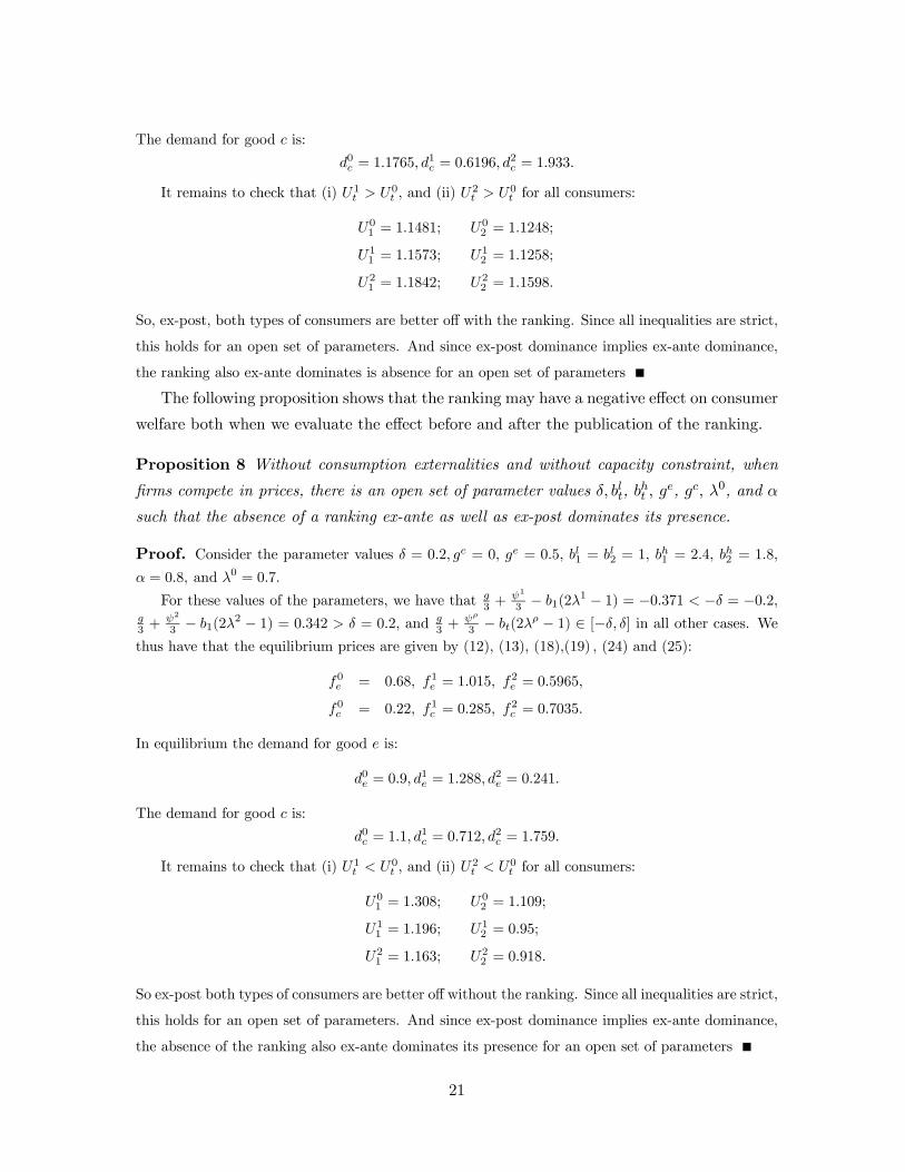
The demand for good c is:
d0c = 1.1765, d1c = 0.6196, d
2c = 1.933.
It remains to check that (i) U1t > U0t , and (ii) U2t > U0t for all consumers:
U01 = 1.1481; U02 = 1.1248;
U11 = 1.1573; U12 = 1.1258;
U21 = 1.1842; U22 = 1.1598.
So, ex-post, both types of consumers are better off with the ranking. Since all inequalities are strict,
this holds for an open set of parameters. And since ex-post dominance implies ex-ante dominance,
the ranking also ex-ante dominates is absence for an open set of parameters
The following proposition shows that the ranking may have a negative effect on consumer
welfare both when we evaluate the effect before and after the publication of the ranking.
Proposition 8 Without consumption externalities and without capacity constraint, when
firms compete in prices, there is an open set of parameter values δ, blt, bht , g
e, gc, λ0, and α
such that the absence of a ranking ex-ante as well as ex-post dominates its presence.
Proof. Consider the parameter values δ = 0.2, gc = 0, ge = 0.5, bl1 = bl2 = 1, bh1 = 2.4, b
h2 = 1.8,
α = 0.8, and λ0 = 0.7.
For these values of the parameters, we have that g3 +
ψ1
3 − b1(2λ1 − 1) = −0.371 < −δ = −0.2,
g3 +
ψ2
3 − b1(2λ2 − 1) = 0.342 > δ = 0.2, and g
3 +ψρ
3 − bt(2λρ − 1) ∈ [−δ, δ] in all other cases. We
thus have that the equilibrium prices are given by (12), (13), (18),(19) , (24) and (25):
f0e = 0.68, f1e = 1.015, f2e = 0.5965,
f0c = 0.22, f1c = 0.285, f2c = 0.7035.
In equilibrium the demand for good e is:
d0e = 0.9, d1e = 1.288, d
2e = 0.241.
The demand for good c is:
d0c = 1.1, d1c = 0.712, d
2c = 1.759.
It remains to check that (i) U1t < U0t , and (ii) U2t < U0t for all consumers:
U01 = 1.308; U02 = 1.109;
U11 = 1.196; U12 = 0.95;
U21 = 1.163; U22 = 0.918.
So ex-post both types of consumers are better off without the ranking. Since all inequalities are strict,
this holds for an open set of parameters. And since ex-post dominance implies ex-ante dominance,
the absence of the ranking also ex-ante dominates its presence for an open set of parameters
21

This result shows that the flexibility of prices does not solve the problem of rankings as
identified in the previous section. On the contrary, with flexible prices the ranking might
create an additional problem for the consumers because it could increase the market power
of the individual firms.
5 Conclusion
In this paper we have demonstrated that the existence of a ranking can be harmful to all
consumers when the good is rationed, when there are consumption externalities, and/or
when firms have market power. These harmful effects are more likely the more random
the rationing procedure is, the more important consumption externalities are, and the more
important the good’s intrinsic quality is relative to the consumers’ idiosyncratic preferences
for a particular good. It seems plausible that markets for study programs rationing, ex-
ternalities, and intrinsic quality play an important role. The same holds e.g. for medical
services. Hence, in these markets it is a-priori unclear whether rankings are beneficial for
consumers or not. But of course the analysis of the existence and the size of harmful effects
of rankings for a particular market is left for future empirical research.
References
[1] Anderson, S., and R. Renault (2009), Comparative Advertising: Disclosing Horizontal
Match Information,RAND Journal of Economics , 40(3), 558-581.
[2] Dranove, D., D. Kessler, M. McClellan, and M. Satterthwaite (2003), Is More Infor-
mation Better? The Effects of "Report Cards" on Health Care Providers, Journal of
Political Economy 111(3), 555-588.
[3] Gavazza, A., and A. Lizzeri (2007), The Perils of Transparency in Bureaucracies, Amer-
ican Economic Review 97(2), Papers and Proceedings, 300-305.
[4] Glazer, J., and T. McGuire (2006), Optimal Quality Reporting in Markets for Health
Plans, Journal of Health Economics 25, 295-310.
[5] Kalaitzidakis, P., T. Mauneas, and T. Stengos (2010), An updated ranking of academic
journals in economics, mimeo.
[6] Morris, S., and H.S. Shin (2002), Social Value of Public Information, American Economic
Review 92(5), 1521-1534.
22

[7] Palacios-Huerta, I., and O. Volij (2004), The measurement of intellectual influence,
Econometrica 72, 963-977.
[8] Sorensen, A. (2007), Bestseller Lists and Product Variety, Journal of Industrial Eco-
nomics 55(4), 715-738.
6 Appendix
:Proof of Proposition 1. Lemma 2 shows that the list of cases of the proposition is exhaustive.
We prove the different cases sequentially.
1. b1(2λρ − 1) > b2(2λ
ρ − 1) implies that
b1(2λρ − 1) + q(x, y) > b2(2λ
ρ − 1) + q(x, y). (26)
We have to distinguish between the following cases:
(a) The condition guarantees that type 2 consumers’ optimal choice is e. Due to (26) it is
also guaranteed that type 1 consumer’s optimal choice is e (see condition (4))
(b) If x∗2 solves
b2(2λρ − 1) + q(1, x∗2) = g,
type 2 consumers are indifferent between applying for the good e and c. Due to (26)
type 1 consumers’ optimal choice is e.
(c) The two conditions guarantee that e is the optimal strategy of consumers of type 1 and
c the optimal strategy of consumers of type 2.
(d) Since x∗1 solves
b1(2λρ − 1) + q(x∗1, 0) = g,
type 1 consumers are indifferent e and c. Due to (26) type 2 consumers’ optimal choice
is c.
(e) The condition guarantees that type 1 consumers’ optimal choice is c. Due to (26) type
2 consumers’ optimal choice is also c.
2. b1(2λρ − 1) < b2(2λ
ρ − 1) implies that
b1(2λρ − 1) + q(x, y) < b2(2λ
ρ − 1) + q(x, y). (27)
We have to distinguish between the following cases:
23

(a) The condition guarantees that type 1 consumers’ optimal choice is e. Due to (27) it is
also guaranteed that type 2 consumer’s optimal choice is e (see condition (4))
(b) If x∗1 solves
b1(2λρ − 1) + q(xρ∗1 , 1) = g,
type 1 consumers are indifferent between applying for the good e and c. Due to (27)
type 2 consumers’ optimal choice is e.
(c) The two conditions guarantee that e is the optimal strategy of consumers of type 2 and
c the optimal strategy of consumers of type 1.
(d) Since x∗2 solves
b2(2λρ − 1) + q(0, xρ∗2 ) = g,
type 2 consumers are indifferent e and c. Due to (27) type 1 consumers’ optimal choice
is c.
(e) The condition guarantees that type 2 consumers’ optimal choice is c. Due to (26) type
1 consumers’ optimal choice is also c.
Proof of Proposition 2. First, we prove part (i) of the proposition. For generic parameter
values, it holds for ρ = 0, 1, 2 that
bt(2λρ − 1) 6= g.
Hence the equilibria with and without ranking are unique, and all consumers of the same type want
the same good. Since there is no capacity constraint, each consumer gets his preferred good.
We have to distinguish between two cases. First, it might be that in equilibrium all consumers
opt for the same good without ranking, with confirmative ranking, and with a surprising ranking,
i.e. x0∗t = x1∗t = x2∗t . Since there is no capacity constraint, this implies that n0 = n1 = n2. Using
this equation and (6) , (7) , and (8) shows that£λ0α+ (1− λ0)(1− α)
¤U1t (n
1, n2) +£(1− α)λ0 + α(1− λ0)
¤U2t (n
1, n2) = U0t (n0) for all t.
Second, it might be that the ranking induces agents to change their choices. Since λ1 > λ0 > λ2
the only possibilities are that a confirmative ranking induces a switch from the good c to good e
(i.e. n0t = n2t = 0, n1t = 1), or a surprise ranking induces a switch from the good e to good c
(n0t = n1t = 1, n2t = 0). Consider the case where type t agents switch from the good c to good e due
to a confirmative ranking. Therefore
bt(2λ1 − 1) > g,
implying that
btα+ λ0 − 1
1− α− λ0 + 2αλ0> g. (28)
24

For n0t = n1t = 1, n2t = 0, we have£
λ0α+ (1− λ0)(1− α)¤U1t (n
1, n2) +£(1− α)λ0 + α(1− λ0)
¤U2t (n
1, n2)
= λ0(α¡−ge + bht
¢+ (1− α)
¡−gc + blt
¢) +
¡1− λ0
¢(α¡−gc + bht
¢+ (1− α)(−ge + blt)),
and
U0t (n0) = λ0(−gc + blt) +
¡1− λ0
¢(−gc + bht ).
Therefore, condition in (9) boils down to£λ0α+ (1− λ0)(1− α)
¤U1t (n
1, n2) +£(1− α)λ0 + α(1− λ0)
¤U2t (n
1, n2)− U0t (n0)
= λ0α¡−ge + bht + gc − blt
¢+ (1− λ0)(1− α)
¡gc − bht − ge + blt
¢= λ0α(−g + bt) + (1− λ0)(1− α)(−g − bt). (29)
Hence£λ0α+ (1− λ0)(1− α)
¤U1t (n
1, n2) +£(1− α)λ0 + α(1− λ0)
¤U2t (n
1, n2)− U0t (n0) > 0⇔
bα+ λ0 − 1
1− α− λ0 + 2αλ0> g,
which is guaranteed by (28).
A similar argument can be made for a switch to good c due to a surprise ranking. In this case
bt(2λ2 − 1) < g.
Substituting (2) and noting that α+ λ0 − 2αλ0 > 0 implies
btλ0 − α
λ0 + α− 2λ0α< g. (30)
For n0t = n1t = 1, n2t = 0, we have£
λ0α+ (1− λ0)(1− α)¤U1t (n
1, n2) +£(1− α)λ0 + α(1− λ0)
¤U2t (n
1, n2)
= λ0(α¡−ge + bht
¢+ (1− α)
¡−gc + blt
¢) +
¡1− λ0
¢(α¡−gc + bht
¢+ (1− α)
¡−ge + blt
¢),
and
U0t (n0) = λ0(−ge + bht ) + (1− λ0)(−ge + blt).
Therefore, condition in (9) boils down to£λ0α+ (1− λ0)(1− α)
¤U1t (n
1, n2) +£(1− α)λ0 + α(1− λ0)
¤U2t (n
1, n2)− U0t (n0)
= λ0 (1− α)¡ge − bht − gc + blt
¢+ (1− λ0)α
¡−gc + bht + ge − blt
¢= λ0 (1− α) (g − bt) + (1− λ0)α(g + bt). (31)
Hence£λ0α+ (1− λ0)(1− α)
¤U1t (n
1, n2) +£(1− α)λ0 + α(1− λ0)
¤U2t (n
1, n2)− U0t (n0) > 0⇔
bα− λ0
2αλ0 − α− λ0< g
25

which is guaranteed because of (30).
Second, we prove part (ii) of the proposition. Let gc = 0, ge = 2, bl1 = bl2 = 1, bh1 = 5, b
h2 = 3.2,
α = 1 and λ0 = 0.7. Because of (5) and since there are no capacity constraints, it holds in equilibrium
that n01 = n21 = 0, n11 = 1 and n02 = n22 = 0, n
12 = 1. Inserting into (31) and (29) gives:£
λ0α+ (1− λ0)(1− α)¤U11 (n
1, n2) +£(1− α)λ0 + α(1− λ0)
¤U21 (n
1, n2)− U01 (n0) = 1.4£
λ0α+ (1− λ0)(1− α)¤U12 (n
1, n2) +£(1− α)λ0 + α(1− λ0)
¤U22 (n
1, n2)− U02 (n0) = 0.14
Since both payoff differences are strictly positive, there is an open neighborhood of these para-
meter values such that the ranking dominates its absence
26