Goodness-of-fit criteria for survival data - uni-muenchen.de · A major interest of survival analysis is the investigation and rating of prog- ... Goodness of ﬁt criteria for survival

Müller:

Goodness-of-fit criteria for survival data

Sonderforschungsbereich 386, Paper 382 (2004)

Online unter: http://epub.ub.uni-muenchen.de/

Projektpartner

http://www.stat.uni-muenchen.de/

http://www.gsf.de/

http://www.mpg.de/

http://www.tum.de/

Goodness of fit criteria for survival data

Martina Müller1

Institute for Medical Statistics and Epidemiology, IMSETechnical University Munich, Ismaningerstr.22, 81675 München, Germany

ABSTRACT

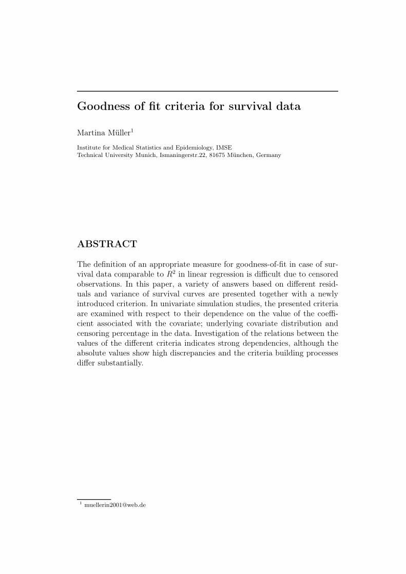
The definition of an appropriate measure for goodness-of-fit in case of sur-vival data comparable to R2 in linear regression is difficult due to censoredobservations. In this paper, a variety of answers based on different resid-uals and variance of survival curves are presented together with a newlyintroduced criterion. In univariate simulation studies, the presented criteriaare examined with respect to their dependence on the value of the coeffi-cient associated with the covariate; underlying covariate distribution andcensoring percentage in the data. Investigation of the relations between thevalues of the different criteria indicates strong dependencies, although theabsolute values show high discrepancies and the criteria building processesdiffer substantially.

1 [email protected]

2 Müller

1 Introduction

A major interest of survival analysis is the investigation and rating of prog-nostic factors for specific diseases. Survival analysis as time-to-event modelsis often realised by semiparametric Cox regression which does not allow fordirect computation of a measure of goodness-of-fit such as R2 for linearregression due to incomplete observation times i.e. censored failure times.Several attempts were made to establish an at least comparable measure.An appropriate measure should represent the difference between the realdata and the predicted values of the model and be dependent on the es-timated coefficients. In addition, it should be able to be interpreted as apercentage of variation in the data that explained by the model. Some ofthe proposed measures have recently been corrected to reduce dependenceon the percentage of censoring in the data.The aim of this paper is to investigate the latest measures along with anewly introduced variant in univariate simulation studies. They will be anal-ysed with respect to their dependence on underlying covariate distribution,strength of the covariate’s influence, which is the associated coefficient, andcensoring percentage in the data. The absolute values of the different mea-sures show high discrepancies. As they all are constructed for the same pur-pose, the associations between the values of the different measures resultingfrom simulated data were examined. It was found that they are stronglyrelated to each other although they are based on different outcomes of sur-vival analysis.In section two, the background of survival analysis, a general definition of R2

and desirable properties of an appropriate measure are outlined. In sectionthree, the definitions of existing criteria along with a newly introduced vari-ant, which measure the goodness-of-fit in survival analysis, are presented.Simulation results are shown and discussed in section four, and in sectionfive, an application to real data is given.

2 Background

2.1 Survival analysis

The main interest of survival analysis is usually the probability to surviveuntil a chosen point on the time axis. This is described by the survivorfunction S(t). The cumulated probability to die until time t, F (t), is relatedto the survivor function by:

S(t) = 1 − F (t)

The hazard function λ(t) represents the instantaneous probability to die attime t+δt for a subject that survived at least until t. The cumulated hazardΛ(t) =

∫ t0 λ(s)ds is related to the survival function by:

Goodness of fit criteria for survival data 3

S(t) = exp(−Λ(t))

The estimation of the survival function can be realised nonparametrically byKaplan-Meier estimator (Kaplan & Meier, 1958). For each point of the timeaxis, the probability of death is calculated as the number of events di relativeto the number R(ti) of subjects at risk at time ti. Hence, censored failuretimes enter the estimation as a reduction in the corresponding number ofsubjects at risk. The Kaplan-Meier estimator is written:

SKM(t) =t∏

i=0

(1 − di

R(ti))

A Kaplan-Meier survival curve is therefore a step function over time withsteps at each time an event occurs, i.e. each failure time. In case of discretecovariates, survival curves for different factor levels can be calculated andcompared by logrank test which gives an indication of the relevance of thefactor, i.e. whether survival in the groups significantly differs.Continuous as well as discrete covariates can be handled by the semipara-metric Cox proportional hazards model (Cox, 1972). This model assumes ageneral baseline hazard λ0(t) for all subjects, given that all covariates haveoutcome zero. This baseline hazard is arbitrary over time t. Nonzero covari-ate values result in a constant shift of this baseline hazard over time.Some software packages, such as S-plus, use mean covariate values for thecalculation of the baseline hazard instead of zero which results in a constantshift of this function. The knowledge of the used reference is only importantfor the interpretation of the resulting baseline hazard function.The assumption of a constant shift of the baseline hazard by covariate val-ues is called proportional hazards and must be checked before interpretingthe results of a Cox regression. If it is not fulfilled, a different model mustbe applied, e.g. one allowing for time-varying coefficients. For a valid Coxmodel, the formula for the hazard function is given as:

λ(t|x) = λ0(t) exp(β ′X)

Estimation in Cox regression is based on the partial likelihood function whichis the first part of the full likelihood and independent of the underlying base-line hazard (Cox, 1975). It has been shown to have similar features as thefull likelihood although some information is lost by reducing the full likeli-hood to its first term. The loss of information is not negligible for small datasets and for informative censoring. It is usually assumed that censored ob-servations do not contribute additional information to the estimation. Thisis the case, if censoring is independent of the survival process. Otherwise,censoring is informative and estimation via partial likelihood is biased.If the data set is large enough and censoring is uninformative, estimation inproportional hazards regression is established by maximising the logarith-mised partial likelihood, which is:

4 Müller

ln PL(β, X) =∑

Yiuncensored

⎛⎝Xiβ − ln∑tj≥ti

exp(β ′Xj)

⎞⎠For tied failure times, a correction must be introduced. Breslow (1974) pro-posed the following correction of the partial likelihood function:

ln PL(β, X) =∑

Yiuncensored

⎛⎝siβ − di

⎡⎣ln ∑tj≥ti

exp(β ′Xj)

⎞⎠⎤⎦Herein, si is the sum of the covariates of all individuals and di is the totalnumber of individuals failing at the ith failure time.Maximisation is realised by setting the score function, which is the firstderivative of the logarithmised partial likelihood, to zero. The score func-tion is:

U(β, X) =∑

Yiuncensored

(Xi −

∑tj≥ti Xj exp(Xjβ)∑

tj≥ti exp(Xjβ)

)

Cox regression has become the standard for survival analysis. However, inpractise, the assumption of proportional hazards is rarely checked althougha wide choice of models allowing for non-proportional hazards by accountingfor time-dependent effects β(t) has been proposed. An example is given byBerger et al. (2003) who model time-dependent effects by fractional poly-nomials.

2.2 Goodness-of-fit criteria

A range of measures of goodness-of-fit and their application for differentsettings are described by Kvalseth (1985). In ordinary linear regression, R2,based on the residual sum of squares, is often the chosen measure for judgingthe fit of a model. It results from the decomposition of sums of squares whereSST is defined as total sum of squares, SSR as the residual sum of squaresand SSM as the sum of squares explained by the model:

R2 =SSM

SST=

SST − SSR

SST= 1 − SSR

SST

However, this measure cannot be used for proportional hazards regressionas the outcome contains incomplete failure times. The definition of residualsfor these models is more complicated and a variety of answers is available.Some of which have been used to create criteria measuring the influence ofthe covariates. The resulting criteria definitions are presented, along withothers, which are not based on residuals, and a newly introduced variant,in the next chapter.General desirable properties of a measure similar to R2 in linear regressionhave been formulated by Kendall (1974). These are:


• R2 = 0 in absence of association• R2 = 1 for perfect predictability• R2 should increase with the strength of association

These three stipulations should be checked within the simulation section forthe presented criteria. Other desirable properties are that the value shouldincrease with the absolute value of the coefficient associated with the ex-amined covariate, and that the measure should not be influenced by thepercentage of censoring in the data. The latter of these properties is noteasy to solve. Although some of the existing measures have been correctedrecently, the simulation results for the new measures indicate that depen-dencies on the censoring percentage are weaker but still exist.

3 Criteria definitions

3.1 Measures based on martingale and deviance residuals

Martingale residuals are defined as the difference between the cumulativehazard assigned to an individual with failure time ti and its observed status,δi = 0 censored, δi = 1 event. Martingale residuals are written as follows(Therneau, Grambsch, Fleming, 1990):

Mi = δi − Λ(ti)

As the cumulative hazard Λ(ti) has no upper limit, these residuals range be-tween 1 and −∞. However, the sum of all martingale residuals is always 0.Λ(ti) is the number of expected events per individual failing at ti accordingto the model. In a perfect model, which is defined as a perfect predictionfor all individuals, all martingale residuals are 0 and uncorrelated to eachother. There is a slight negative correlation in all other models due to theproperty that they sum up to 0.A high Λ(ti) can be interpreted as a high indication of death and will resultin a highly negative martingale residual. According to the model, these in-dividuals were under observation for too long. As Λ(t) increases with time,the residuals will tend towards increasingly negative values for longer ob-servation times and have a highly skewed distribution.Normalised transformations of martingale residuals have therefore been de-fined. These transformed versions are called deviance residuals:

devMi = sgn(Mi)√−2(Mi + δi ln(δi − Mi))

This definition resembles the definition of deviance residuals in Poisson re-gression, but as the nuisance parameter, the unspecified baseline hazardλ0(t) is still involved, and the squared residuals do not exactly sum up to

6 Müller

the deviance of the model, as they would do for Poisson regression (Venables& Ripley, 1997). Hence, the sum of squared residuals cannot be interpretedas the total deviance of the model.Martingale residuals can be used to detect the functional form of a covari-ate. Outlier screening can be performed by plotting either kind of residualagainst time but this may be established more easily by using devianceresiduals.Especially for covariate models with high coefficients and low censoring per-centage, martingale residuals tend towards extreme negative values.A common property of these residuals is their high dependence on theamount of censoring in the data. The survival function is always calcu-lated with respect to the amount of subjects at risk. Censoring by means ofthe end of a study will always increase the probability that a subject who isexpected to have a long expected survival time is censored in comparison toa subject who is expected to have a short expected survival time. There aretherefore usually more censored observations at the end of the study. Thesurvival function only has steps at times that are marked by failures. If thelast point on the time axis is not a failure, the survival function flattens ear-lier than it would do if the last observation is a failure. This is because onlythe number of individuals at risk at the last observed failure is taken intoaccount. Flattening survival also results in flattening cumulative hazard andtherefore less extreme residuals. On the other hand, extreme residuals occurfor high cumulative hazards. Consequently, these can be obtained in casesof low censoring or high values of the product of covariates and associatedcoefficients, i.e. the linear predictor.Adopting the idea of a goodness-of-fit criterion based on residual sums ofsquares, comparable to R2 in linear regression, will often result in the pref-erence of a null model over any covariate model. This is because the squaredextreme residuals resulting from high values of the linear predictor increasethe sum of squares to such extremes that R2, which includes the differencebetween the sum of squares of residuals from null and covariate model, caneven yield high negative values. The assumption of having normally dis-tributed residuals, which is needed for the application of R2, is simply notfulfilled because the distribution of martingale residuals is more exponen-tially shaped. This also applies to the more normally distributed devianceresiduals - weaker but still visible.Hence, a different definition for an appropriate criterion is needed. Stark(1997) proposed measuring the mean absolute differences between residualsof null and the covariate model and setting the sum relative to the mean ofabsolute residuals of the null model. Thus, with Mi|x as martingale residualin the covariate model and Mi as residual of the null model, the new mea-sure is written:


Km.norm =

1n

∑i

∣∣∣Mi − Mi|x∣∣∣

1n

∑i |Mi| =

∑i

∣∣∣Λi − Λi|x∣∣∣∑

i |Mi|

Note that the observed status cancels in the counter of the fraction whencalculating absolute differences.For deviance residuals an analogous measure can be built:

Kd.norm =

1n

∑i

∣∣∣devMi − devMi|x∣∣∣

1n

∑i |devMi| =

∑i

∣∣∣devMi − devMi|x∣∣∣∑

i |devMi|

This new definition does not completely circumvent problems arising fromthese types of residuals. Although negative values are avoided, the differ-ences between the residuals of the two models may still get very high, i.e.the difference between two residuals resulting from the two applied modelsmay be larger than the residual of the null model. In this case, often themeasures can exceed the maximum value allowed for a goodness-of-fit crite-rion, which is 1 (Kendall, 1975). Simulation studies presented later showedthat these problems arise especially for data with low censoring percentageand high discrepancies of the linear predictor. The latter case occurs if thetrue underlying covariate distribution allows for high variance of covariatevalues in combination with a high coefficient.Correction is difficult, but will be the object of further research.

3.2 Measures of variation in survival

As survival can be taken as a major point of interest, criteria have beenproposed that are based on the survival function. Initially, the absolute dis-tance or the mean squared distance between the survival curves of a nullmodel obtained through Kaplan-Meier estimation and a covariate includingCox model were measured (Schemper, 1990).These were later improved by measuring the weighted reduction of variancein the survival processes (Schemper & Henderson, 2000). The variance ofthe individual survival process at time t is defined as S(t) {1 − S(t)} fora null model and S(t|X) {1 − S(t|X)} for the covariate model (Schemper& Henderson, 2000). The mean absolute deviation measures are definedas 2S(t) {1 − S(t)} and 2S(t|X) {1 − S(t|X)}. Measures of predictive accu-racy integrated over the full follow-up range are weighted by a function oftime to reduce dependence on censoring and the factor 2 is dropped as itcancels in the resulting criteria definitions. Hence:

D(τ) =

∫ τ0 S(t) {1 − S(t)} f(t)dt∫ τ

0 f(t)dt

Dx(τ) =

∫ τ0 EX [S(t|X) {1 − S(t|X)}] f(t)dt∫ τ

0 f(t)dt

8 Müller

The measure V of the relative gain is then formulated. It is written as thedifference between the variance in survival for the null model, D, and itsexpectation for the covariate model, Dx, relative to that of the null model:

V (τ) =D(τ) − Dx(τ)

D(τ)

An alternative formulation is defined using weighted relative gains. Theweighting functions are moved as follows:

VW (τ) =

∫ τ0

S(t){1−S(t)}−EX [S(t|X){1−S(t|X)}}S(t){1−S(t)} f(t)dt∫ τ

0 f(t)dt

For estimation, S(t) {1 − S(t)} and EX [S(t|X) {1 − S(t|X)}] must be splitinto three terms at each distinct death time t(j) as there are individuals stillalive (line 1 below), individuals that died before t(j) (line 2) and those whoare censored before t(j) (line 3). The mean absolute distance measure D istherefore estimated by M(t(j)) as follows:

M(t(j)) =1

n

n∑i=1

[I(ti > t(j))

{1 − S(t(j))

}+δiI(ti ≤ t(j))S(t(j))

+(1 − δi)I(ti ≤ t(j))

{(1 − S(t(j)))

S(t(j))

S(ti)+ S(t(j))

(1 − S(t(j))

S(ti)

)}]

Dx is calculated the same way as D only with survival estimates S(t(j))

replaced by S(t(j)|X), which are obtained from a Cox model.In the next step, the weights are calculated from the potential follow-updistribution, also called reverse Kaplan-Meier, which is estimated like aKaplan-Meier estimator for survival, but with the meaning of the status in-dicator δ reversed (Schemper & Smith, 1996 and Altman et al., 1995). Thereverse Kaplan-Meier function is denoted G. With dj being the number ofdeaths at time t(j), the weights at time t(j) are defined as follows:

wj =dj

G(t(j))

Hence, the estimate V = (D − Dx)/D is calculated with:

D =

∑j wjM(t(j))∑

j wjand Dx =

∑j wjM(t(j)|x)∑

j wj

And VW is:


VW =

∑mj=1 wj

M(t(j))−M(t(j) |x)

M(t(j))∑j wj

Simulation studies showed that the value of VW is always slightly smallerthan V .

3.3 Measures based on Schoenfeld residuals

A different method for judging a model is based on Schoenfeld residuals(Schoenfeld, 1982). These measure the model’s accuracy in a different way.At all complete failure times, the true covariates assigned to an individualfailing are compared to the expected value of the covariate under the model,assuming the model is true. Hence, the idea is completely different from themeasures presented so far. While martingale residuals and the variance ofthe survival curves are calculated conditioning on the covariates, these resid-uals investigate covariate values conditioning on time. The expected valuesof the covariates are calculated with respect to the probabilities assigned tothe values by the model. With ri(t) as indicator whether individual i is stillat risk at time t, the Schoenfeld residuals are defined as follows:

rschi(β) = Xi(ti) − E(Xi(ti)|β)

= Xi(ti) −n∑

j=1

Xj(ti)πj(β, ti)

= Xi(ti) −n∑

j=1

Xj(ti)rj(ti) exp(β ′Xj(ti))∑n

j=1 rj(ti) exp(β ′Xj(ti))

Consequently, when calculating these residuals, the result will be a matrixwith the number of rows equalling the number of events and a column percovariate.In order to define a measure for the goodness-of-fit of the model a modi-fied version of residuals is needed for a null model. This is difficult becausethe residual is based on the covariates. For the null model, the covariate issupposed to have no influence and can be assigned to the individuals ar-bitrarily. Therefore, residuals for the null model are obtained by replacingthe probability πj(β, ti) in the upper definition for the covariate model byπj(0, ti) = rj(ti)/

∑nj=1 rj(ti). In this way, all covariate values have the same

probability and there is no preference for values as in a covariate model. Afirst measure for the goodness-of-fit has been formulated based on squaredresiduals (O’Quigley & Flandre, 1994):

R2OF =

∑ni=1 r2

schi(0) −∑n

i=1 r2schi

(β)∑ni=1 r2

schi(0)

10 Müller

= 1 −∑n

i=1 r2schi

(β)∑ni=1 r2

schi(0)

The next problem is that the residuals are calculated per covariate and itis difficult to judge multivariate models. The idea of the prognostic index(Andersen et al., 1983) has therefore been adopted as each patient’s outcomeis dependent of the combination of all covariates. The prognostic index isdefined as:

η(t) = β ′X(t)

Hence, the definition of a criterion, which can also be applied to a multi-variate model, is based on Schoenfeld residuals multiplied by the vector ofcovariates.To reduce dependencies on the censoring percentage in the data, the squaredresiduals are weighted by the height of the increment of the marginal sur-vival curve at the corresponding point on the time axis. This is obtainedfrom the marginal Kaplan-Meier estimate (O’Quigley & Xu, 2001).The weighted version of the new measure R2

sch is then written as follows:

R2sch(β) =

∑ni=1 δiW (ti) {β ′rschi

(0)}2 −∑ni=1 δiW (ti) {β ′rschi

(β)}2∑ni=1 δiW (ti) {β ′rschi

(0)}2

= 1 −∑n

i=1 δiW (ti) {β ′rschi(β)}2∑n

i=1 δiW (ti) {β ′rschi(0)}2

The weights W (ti) are the height of the step of the marginal Kaplan-Meiersurvival curve at time ti; rschi

(β) is the Schoenfeld residual for the covariatemodel and rschi

(0) the residual for the null model.R2

sch(β) is a consistent estimate for Ω2(β), which is a measure of explainedvariation for X|t (O’Quigley & Xu, 2001). The expected minimum is 0 andthe maximum is 1 while R2

sch(β) is increasing with β. Another advantage ofthis formulation is that asymptotically, decomposition into residual sums ofsquares is possible, as for linear models:

SSTasympt.

= SSR + SSM

with

SST =n∑

i=1

δiW (ti){β ′rschi

(0)}2

SSR =n∑

i=1

δiW (ti){β ′rschi

(β)}2

SSM =n∑

i=1

δiW (ti){β ′Eβ(Xti) − β ′E0(X|ti)

}2

Apart from these properties, this formulation allows for an easy extension


to nested, stratified and time-varying models. An overview of possible ex-tensions and proofs are given in Xu (1996), Xu & O’Quigley (2001) and Xu& Adak (2002).For comparison reasons, a new variant based on Schoenfeld residuals isintroduced which is generally constructed like the measures based on cu-mulative hazards while the weighting is kept. The mean absolute differencebetween the residuals of the two models is therefore calculated, weightedand divided by the mean of weighted absolute residuals of the null model.The new measure is written:

R2sch.k(β) =

1n

∑ni=1 δiW (ti) |β ′rschi

(0) − β ′rschi(β)|

1n


(0)|

=


(0) − β ′rschi(β)|∑n

i=1 δiW (ti) |β ′rschi(0)|

Being aware that some desirable properties of R2sch(β) are lost by this new

formulation, this measure is mainly introduced to draw a comparison withKm.norm and Kd.norm.

12 Müller

4 Simulation studies

4.1 Data simulation

In simulation studies, the presented measures were analysed with respect totheir dependence on coefficients β, distribution of the covariate X and cen-soring percentage in the data. In addition, relations between the outcomesof the different measures were investigated.Computation of the measures was based on data sets consisting of 1000observations with exponentially distributed failure time tf and expectationE(tf |X, β) = 1/ exp(β ′X). Uninformative censoring was added, comparableto clinical studies where patients enter continuously over time and the studyis stopped after a predefined maximum observation time or after a certainnumber of events is reached. Therefore, a uniformly distributed censoringtime was created for each subject, tcU(0, τ). The observation time is takenas the minimum of tf and tc, the status indicator is set to 1 for tf ≤ tc andzero otherwise. The upper limit τ was varied to obtain censoring percentagesof 0% and approximately 10%, 25%, 50% and 80%. Hence, the influence ofincreasing censoring can be investigated.Distributions of X were initially chosen as binary with p = 0.5, uniformXU(0,

√3) and normal XN(0, 0.25) as these three distributions have the

same variance although they differ in expectation. Additionally, more stan-dard distributions were chosen, XN(0, 1) and XU(0, 1). The former of whichresults in higher variance of X with values centred at 0 while the latter willhave lower variance than the binary covariate. The influence of the distri-bution of X can therefore be observed.Each value of X was then associated with different coefficients chosen fromthe set β ∈ {0.5, 1, 2, 3} to yield failure times.For each of the five covariate distributions, 200 data sets of 1000 observa-tions along with one failure time and four different censoring times for eachvalue of β were generated. Hence, each measure was calculated 200 timesfor each setting defined by covariate distribution, value of β and censoringpercentage.

4.2 Criteria investigation

All criteria were initially calculated for the data sets with binary X. Theobtained criteria are plotted against the according coefficients β in figure 1.Lines are drawn between the means at each value of β with different stylesfor different censoring percentages in the data. Correlations between β andthe values of all the criteria are high. The maximum correlation is 0.995and is reached by R2

sch for data without censoring whereas the minimum is0.910 and is obtained for VW in the data with 80% censoring.As can be seen in figure 1, all criteria grow with increasing values of β, which


beta

k.m

.nor

m

0.5 1.0 2.0 3.0

0.0

0.2

0.4

0.6

0.8

1.0

k.m.norm for X~bin

beta

k.d.

norm

0.5 1.0 2.0 3.0

0.0

0.2

0.4

0.6

0.8

1.0

k.d.norm for X~bin

beta

r2.s

ch

0.5 1.0 2.0 3.0

0.0

0.2

0.4

0.6

0.8

1.0

r2.sch for X~bin

beta

r2.s

ch.k

0.5 1.0 2.0 3.0

0.0

0.2

0.4

0.6

0.8

1.0

r2.sch.k for X~bin

beta

V

0.5 1.0 2.0 3.0

0.0

0.2

0.4

0.6

0.8

1.0

V for X~bin

betaV

w

0.5 1.0 2.0 3.0

0.0

0.2

0.4

0.6

0.8

1.0

Vw for X~bin

0% Zens10% Zens25% Zens50% Zens80% Zens

Figure 1. Criteria over different values of coefficient β and varying censoring percentages for

a binary covariate X. The points display the true values; lines are drawn between the criteria’s

means for each coefficient. The lines represent the mean results for different censoring percentages

in the data as indicated in the legend.

is desirable as covariates with high coefficients are more important by meansof prediction. The strength of the increase is, to some extend for all criteria,dependent on the censoring percentage in the data. The measures based onthe variance of the survival curves are less affected by censoring providingthis is not extreme. For high censoring (80%) the factor’s contribution tothe model can only be detected for high coefficients, here β = 3 (figure 1).The measures based on martingale and deviance residuals are more obvi-ously affected by censoring than the others. The strong monotonic decreaseis due to less extreme values of the cumulative hazard in presence of censor-ing. Hence, residuals are less extreme especially for the covariate model, andthe difference between the two models decreases. The Schoenfeld residualmeasures yield the lowest values for 50% of censoring and, in contrast tothe other criteria, highest values for the data with 80% censoring. But theyare generally less affected by censoring than the martingale and devianceresidual measures. However, the values of these criteria have higher variance.

When comparing the absolute values of all criteria, wide differences occur(table 1). For data without censoring and coefficient β = 3, the martingale

14 Müller

residual measure yields an average of 0.886 whereas the mean of VW is 0.314.

Table 1. Mean values of the criteria for 200 simulated data sets per coefficient β without

censoring and binary X.

Measure β = 0.5 β = 1 β = 2 β = 3

K.m.norm 0.315 0.548 0.792 0.886

K.d.norm 0.257 0.471 0.741 0.864

R2.sch 0.060 0.185 0.479 0.712

R2.sch.k 0.184 0.354 0.635 0.811

V 0.027 0.098 0.275 0.400

Vw 0.024 0.084 0.222 0.314

The Schoenfeld residual measures yield values that range between mar-tingale and survival measures. Therefore the criteria are grouped and ageneral ranking can be established which in most cases holds for all testedcovariate distributions:

Km.norm, Kd.norm ≥ R2sch, R

2sch.k ≥ V, VW

In addition, the shape of the trend of the criteria over β can be judged. Forthe measures based on martingale or deviance residuals, the trend over βis more logarithmic whereas the other measures show more linear depen-dencies. This is due to the expected maximum value of 1. It will be seen inother simulation data that as soon as the measures approach 1, the curveflattens for all the criteria.On the other hand, the criterion R2

sch in some cases is slightly negative forβ = 0.5. In these cases the measure presumes that the effect of the covariateis negligibly small i.e. the null model is better than the covariate model. Infact, β = 0.5 is a small coefficient for a binary covariate. The associatedrelative risk would be rr = exp(β) = 1.65. And most of the other criteriaalso yield some values near zero.

The same analysis was then carried out on the continuous covariate dis-tributions. First choice was XU(0,

√3) as this distribution has the same

variance as that of a binary variable with p = 0.5 and differs only slightlyin its expectation. The results are displayed in figure 2. As can be seen,the criteria behave much like those calculated for the data sets with a bi-nary covariate. Only for the measures V and VW the increase with β in thehigh censoring data, 80%, is more linear than for binary data. In addition,there are more extreme values within R2

sch and R2sch.k. Standard deviations

of these criteria increase for high censoring percentages more than for the


others.

beta

k.m

.nor

m

0.5 1.0 2.0 3.0

0.0

0.2

0.4

0.6

0.8

1.0

k.m.norm for X~unif.r3

beta

k.d.

norm

0.5 1.0 2.0 3.00.

00.

20.

40.

60.

81.

0

k.d.norm for X~unif.r3

beta

r2.s

ch

0.5 1.0 2.0 3.0

0.0

0.2

0.4

0.6

0.8

1.0

r2.sch for X~unif.r3

beta

r2.s

ch.k

0.5 1.0 2.0 3.0

0.0

0.2

0.4

0.6

0.8

1.0

r2.sch.k for X~unif.r3

beta

V

0.5 1.0 2.0 3.0

0.0

0.2

0.4

0.6

0.8

1.0

V for X~unif.r3

beta

Vw

0.5 1.0 2.0 3.0

0.0

0.2

0.4

0.6

0.8

1.0

Vw for X~unif.r3



a uniform covariate distribution X(0,√

3). The points display the true values; lines are drawn

between the criteria’s means for each coefficient. The lines represent the mean results for different

censoring percentages in the data as indicated in the legend.

The next data analysed was that with normally distributed covariates,XN(0, 0.25). The values of X are centred at zero but have the same varianceas the other distributions that have already been discussed. The centring ofX at zero leads to lower values in all the criteria as can be seen in figure 3.The measures V and VW hardly yield more than 0.2 and several values ofR2

sch are again slightly negative. X in this setting is therefore not a strongfactor.

The data with XU(0, 1) was then analysed with respect to the model fitcriteria. The expectation of X is the same as for binary X although thevariance is lower. The results are very similar to those for the data withXN(0, 0.25). Hence, no separate plot is displayed. Again, values of V andVW are very low and rarely exceed 0.2. The standard deviations of theSchoenfeld residual measures increase with the censoring percentage in thedata.

16 Müller

beta

k.m

.nor

m

0.5 1.0 2.0 3.0

0.0

0.2

0.4

0.6

0.8

1.0

k.m.norm for X~n0.25

beta

k.d.

norm

0.5 1.0 2.0 3.0

0.0

0.2

0.4

0.6

0.8

1.0

k.d.norm for X~n0.25

beta

r2.s

ch

0.5 1.0 2.0 3.0

0.0

0.2

0.4

0.6

0.8

1.0

r2.sch for X~n0.25

beta

r2.s

ch.k

0.5 1.0 2.0 3.0

0.0

0.2

0.4

0.6

0.8

1.0

r2.sch.k for X~n0.25

beta

V

0.5 1.0 2.0 3.0

0.0

0.2

0.4

0.6

0.8

1.0

V for X~n0.25

betaV

w

0.5 1.0 2.0 3.0

0.0

0.2

0.4

0.6

0.8

1.0

Vw for X~n0.25


Figure 3. Criteria over different values of coefficient β and varying censoring percentages for a

uniform covariate distribution XN(0, 0.25). The points display the true values; lines are drawn



The last analysed data sets are those with a standard normally distributedcovariate. The covariate values are centred at zero but have variance fourtimes as high as the binary covariate. The high variance allows for high val-ues of X. In combination with high coefficients β this leads to high valuesin criteria judging the goodness of fit as can be seen in figure 4.Here, all curves have more or less logarithmic shapes. The values of all

the criteria are much higher than in the cases discussed before. EspeciallyKm.norm and Kd.norm exceed the expected upper limit of 1 for high coeffi-cients. As mentioned before, cumulative hazards increase for strong factorsand lead to extreme residuals such that the absolute difference between theresiduals in the covariate model and those from the null model is higher thanthe absolute residuals calculated for the null model. Therefore an extremeimprovement is obtained. The same observation is made for a few values ofR2

sch.k. The question arises whether this setting is a realistic situation. If so,the fact that the limit of 1 is exceeded requires correction of these criteriaas the property of interpretation as a percentage of explained variation islost otherwise. On the other hand, the values of V and VW are very low for


beta

k.m

.nor

m

0.5 1.0 2.0 3.0

0.0

0.2

0.4

0.6

0.8

1.0

k.m.norm for X~n01

beta

k.d.

norm

0.5 1.0 2.0 3.0

0.0

0.2

0.4

0.6

0.8

1.0

k.d.norm for X~n01

beta

r2.s

ch

0.5 1.0 2.0 3.0

0.0

0.2

0.4

0.6

0.8

1.0

r2.sch for X~n01

beta

r2.s

ch.k

0.5 1.0 2.0 3.0

0.0

0.2

0.4

0.6

0.8

1.0

r2.sch.k for X~n01

beta

V

0.5 1.0 2.0 3.0

0.0

0.2

0.4

0.6

0.8

1.0

V for X~n01

betaV

w

0.5 1.0 2.0 3.0

0.0

0.2

0.4

0.6

0.8

1.0

Vw for X~n01



a uniform covariate distribution XN(0, 1). The points display the true values; lines are drawn



all other distributions of X and need further examination in case the othersettings are more realistic.

18 Müller

Summary

In summary, it is evident that all the criteria strongly depend on the co-efficient associated with the covariate. The measures Km.norm and Kd.norm

decrease constantly with increasing censoring percentages and meanwhile ithas been established in this piece of work that they may exceed the expectedmaximum of 1 for extreme settings.The Schoenfeld residual based measures return the lowest values for 50%censoring in the data and are often highest for 80%. They have generallyhigher variance than the other measures. For low coefficients, R2

sch may beslightly negative, which is an indication for a very weak covariate. In thesecases, the null model is preferred over the covariate model. R2

sch.k, as well asKm.norm and Kd.norm, exceeds the desired maximum value of 1 in extremesettings. Therefore, these criteria cannot be interpreted as a percentage ofexplained variation.V and V w only decrease for high censoring (80%). They are otherwise un-affected by censoring but the values are generally low.All measures highly depend on the true underlying covariate distributionon the basis of which the survival times are created. None of the criteriaare affected by rescaling of the covariate in the criteria calculating process,as they all involve the covariate only in combination with the associatedcoefficient β. Rescaling of the covariate only results in a different value of βduring estimation.


4.3 Relations between the different criteria

As all of the presented criteria are supposed to measure the goodness-of-fitof a model, the next idea was to examine the relations between them. An-alytical descriptions of these are difficult, as the criteria building processesdiffer in number of the terms in the sums and weighting functions are dif-ferent.The criteria resulting from the 800 simulation data sets per covariate distri-bution without censoring (200 per value of β) were therefore plotted againsteach other. Strong relationships occurred. When comparing the plots for allcovariate distributions, the relationships seemed very similar for all con-tinuous covariate distributions. When analysing all criteria for continuousX together (i.e. 3200 values per criterion), correlations ranged between0.9318 and 0.9980 whereas for binary X, correlations ranged between 0.9630and 0.9997. Summing all results of the five distributions together changedthe range of correlations to (0.9313, 0.9970). The plot, however, showed aslightly different trend for the criteria resulting from simulation data withbinary X for several combinations. Hence, it was decided to keep the dis-tinction between continuous and binary covariate distributions.In figure 5, the criteria resulting from simulation data without censoring andcontinuous distributions of X are plotted against each other. The strong re-lationship between the criteria is obvious. The gaps that occur in the plotcan be explained by the discrete values of β. Although the trend is obviousfor all relationships, those which involve R2

sch.k show higher variance.The plot for the data with binary X shows similar trends and compara-bly strong relationships between the criteria. Therefore, it is not displayedseparately. The regions for different values of β, however, are more dis-tinguishable except for the relation between Km.norm and Kd.norm, which isshaped like the relation in figure 5. Again, the relations to R2

sch.k have highervariance.

As no analytical answer to the question of the true form of the rela-tionship is available yet, fractional polynomials were applied to each pair ofcriteria. In this way, a first impression of the relationships and the influenceof censoring percentage, covariate distribution and coefficient on these canbe obtained. Fractional polynomials are defined as follows (Royston & Alt-man, 1994):

FP (x, p) = b0 +m∑

j=1

bjx(pj)

Hence, a polynomial of degree m with exponents p is fit to describe theform of a trend. In practice, a maximum degree of m = 2 and exponentschosen from the set p ∈ {−2,−1,−0.5, 0, 0.5, 1, 2, 3}, with x(0) = ln(x), issufficient for describing most trends. Each exponent can be chosen morethan once. In this case, the first term will be xp and the second is defined

20 Müller

k.m.n.k

k.d.n

.k

0.0 0.2 0.4 0.6 0.8 1.0 1.2

0.0

0.2

0.4

0.6

0.8

1.0

K.m.norm - K.d.norm

k.m.n.kr2

.sch

0.0 0.2 0.4 0.6 0.8 1.0 1.2

0.0

0.2

0.4

0.6

0.8

K.m.norm - R2.sch

k.m.n.k

r2.s

ch.k

0.0 0.2 0.4 0.6 0.8 1.0 1.2

0.2

0.4

0.6

0.8

1.0

K.m.norm - R2.sch.k

k.m.n.k

V

0.0 0.2 0.4 0.6 0.8 1.0 1.2

0.0

0.2

0.4

0.6

K.m.norm - V

k.m.n.k

Vw

0.0 0.2 0.4 0.6 0.8 1.0 1.2

0.0

0.1

0.2

0.3

0.4

0.5

0.6

K.m.norm - Vw

k.d.n.k

r2.s

ch

0.0 0.2 0.4 0.6 0.8 1.0

0.0

0.2

0.4

0.6

0.8

K.d.norm - R2.sch

k.d.n.k

r2.s

ch.k

0.0 0.2 0.4 0.6 0.8 1.0

0.2

0.4

0.6

0.8

1.0

K.d.norm - R2.sch.k

k.d.n.k

V

0.0 0.2 0.4 0.6 0.8 1.0

0.0

0.2

0.4

0.6

K.d.norm - V

k.d.n.k

Vw

0.0 0.2 0.4 0.6 0.8 1.0

0.0

0.1

0.2

0.3

0.4

0.5

0.6

K.d.norm - Vw

r2.sch

r2.s

ch.k

0.0 0.2 0.4 0.6 0.8

0.2

0.4

0.6

0.8

1.0

R2.sch - R2.sch.k

r2.sch

V

0.0 0.2 0.4 0.6 0.8

0.0

0.2

0.4

0.6

R2.sch - V

r2.sch

Vw

0.0 0.2 0.4 0.6 0.8

0.0

0.1

0.2

0.3

0.4

0.5

0.6

R2.sch - Vw

r2.sch.k

V

0.2 0.4 0.6 0.8 1.0

0.0

0.2

0.4

0.6

R2.sch.k - V

r2.sch.k

Vw

0.2 0.4 0.6 0.8 1.0

0.0

0.1

0.2

0.3

0.4

0.5

0.6

R2.sch.k - Vw

V

Vw

0.0 0.2 0.4 0.6

0.0

0.1

0.2

0.3

0.4

0.5

0.6

V - Vw

Figure 5. Criteria for continuous distributions of X for data without censoring plotted against

each other show strong relationships.

as ln(x)x(p). Consequently, a fractional polynomial of degree m = 2 withexponents p = (0, 3) for example is written:

FP (x, p = (0, 3)) = b0 + b1 ln(x) + x3

The optimal fractional polynomial is found stepwise starting from the mostcomplex model with m = mmax. This is compared to the best model ofdegree m = mmax − 1. The procedure stops as soon as the deletion of aterm results in a significant change in deviance.

The goodness-of-fit of a fractional polynomial model is measured by residualdeviance, which is also the measure of choice for judging the goodness-of-fitof generalised linear models. A good fit is achieved if the residual devianceis small. The residual deviances, along with the corresponding number ofresidual degrees of freedom, are displayed in table 2 for the two data sets.Compared to the number of observations and remaining residual degrees offreedom, the residual deviance is generally small. This can be seen in table2 and therefore gives an indication for a good fit. As already pointed outin the discussion of the plots, the highest variance occurs for relations to


Table 2. Residual deviances resulting from fractional polynomial fits between the criteria cal-

culated for continuous distributions of X and binary X respectively.

Model Residual deviance Residual deviance

X cont. X bin.

Residual df = 3197 Residual df = 797

Kd.norm

Km.norm 0.1531 0.0857

R2

schKm.norm 0.5202 0.3154

R2

sch.kKm.norm 2.4110 0.4277

VKm.norm 0.2219 0.0916

VW

Km.norm 0.4758 0.0436

R2

schKd.norm 0.7038 0.0359

R2

sch.kKd.norm 2.5195 0.1514

VKd.norm 0.2479 0.0055

VW

Kd.norm 0.5925 0.0017

R2

schR2

sch.k 1.6436 0.2189

R2

schV 0.1793 0.0259

R2

schVW 0.2915 0.0165

VR2sch.k 1.0901 0.0690

VW

R2sch.k 1.3063 0.0374

VVW 0.1859 0.0011

R2sch.k, which is proved by higher residual deviances. The relation, however,

is strong.

Variance in the plot increased with censoring in the data, especially forrelations to the Schoenfeld residual measures. The trend between the twocriteria based on cumulative hazards and that between the measures V andVW remained practically unchanged, which indicates similar dependencieson censoring for these criteria. The reason for the high variance is obviouslythe higher variance that has been observed for the criteria R2

sch and R2sch.k.

Km.norm and Kd.norm, however, are strongly dependent on censoring. There-fore, the relation to the other criteria is increasingly compressed, althoughthe general shape of the trend is kept.As for the data with binary X, the detection of a trend for relations in-volving V or VW is difficult for 80% censored observations per data set. Asalready mentioned in the discussion of figure 1, these criteria only detectthe covariate when it is combined with a high coefficient. The trend over βis not smooth. Consequently, the relation to the other criteria is not smootheither.

22 Müller

4.4 Discussion of simulation results

The presented criteria judge the goodness-of-fit of a survival model withrespect to different outcomes, as there are cumulative hazard; predictionof covariates, and variance of survival curves. All depend strongly on theassociated coefficient and the distribution of the true underlying covariate.However, they differ strongly in value. While the measures V and VW aregenerally very small, the criteria based on cumulative hazard tend to exceedthe expected maximum value of 1 for strong factors in data sets with verysmall censoring percentages. The latter measures are the only ones that ob-viously decrease monotonically with increasing censoring in the data. R2

sch.k

also exceeds the desired maximum value of 1, and it therefore does not al-low for interpretation as a percentage. R2

sch for weak factors occasionallyyields slightly negative values, although its minimum in expectation is 0. Inaddition, the measures based on Schoenfeld residuals have higher variancethan all the other criteria presented here. Consequently, all of the measuressuffer drawbacks.However, strong relations between all of the criteria could be detected. Whendescribing these, data with binary X had to be distinguished from data withcontinuous X. For further specification of the trends the censoring percent-age has to be taken into account. This is especially the case for relationsincluding Km.norm and Kd.norm. Once this is realised, the successful cal-culation of at least one of the measures should allow for the subsequentderivation of all remaining measures. The precision of covariate predictionis therefore directly related to the gain of explained variation in the survivalcurves and the precision of cumulative hazards.

5 Application to stomach cancer data

The data analysed originate from a clinical study from Chirurgische Klinikder TU München during the years 1987 and 1996. 295 patients with stomachcancer were analysed with respect to their survival. The maximal individualfollow-up time is 11 years. The censoring percentage in the data is 63%. Inearlier analyses with less data (Stark, 1997), a dichotomised version of thepercentage of seized lymph nodes (NODOS.PR) was identified as strongestprognostic factor. The optimal version of NODOS.PR is now recalculated forthe new data and analysed with respect to its contribution to the goodness-of-fit of the model by means of the presented criteria.

For a complete analysis, assumptions for the application of a Cox modelmust be checked first. These include linearity (if necessary, combined withthe finding of the optimal functional form) of the covariate and proportionalhazards. Initially, a varying coefficient model (Hastie & Tibshirani, 1993) isfit using a spline of NODOS.PR as covariate to check for linearity. As can


Figure 6. The varying coefficients spline plot for the continuous covariate NODOS.PR shows

that the linearity assumption is violated. No linear trend is possible within the 95% confidence

region (dashed lines). Vertical lines indicate possible positions for dichotomisation.

be seen in figure 6, no linear effect is possible within the 95% confidence re-gion (dashed lines) and a dichotomised version of NODOS.PR is preferablewhich distinguishes between a low risk and a high risk group.Another indication for dichotomisation was found in the check of the func-tional form of NODOS.PR. This graphical check is established by plottingmartingale residuals of the null model against the values of NODOS.PR (Th-erneau & Grambsch, 2000). The smoothed fit is monotonic and logisticallyshaped (figure 7), which is an indication for a threshold, and a dichotomi-sation is proposed.The optimal cut point was found by simultaneously testing all data pointsin NODOS.PR, that guarantee at least ten individuals per group, as can-didate split points. Test statistic is the logrank statistic, which is adjustedfor multiple testing according to Lausen & Schumacher (1992). The optimalcut point is found as the one with minimum p-value. Here, the two minimalp-values have been picked. The according cut points lead to two differentbinary covariates that were tested with respect to their contribution to themodel fit. The optimal cut point was found at 0.1212, the next best point fordichotomisation is at 0.2326. Both log rank statistics are highly significanteven after adjusting the p-values for multiple testing. The new covariatesare named nod.122 and nod.24.Next, the assumption of proportional hazards was checked using the methodproposed by Grambsch & Therneau (1994), which tests for correlation be-tween time, or transforms of time, and scaled Schoenfeld residuals. Here,

24 Müller

NODOS.PR

Mar

tinga

le re

sidu

als

from

nul

l mod

el

0.0 0.2 0.4 0.6 0.8 1.0

-0.5

0.0

0.5

1.0

Figure 7. Martingale residuals obtained from the null model plotted against the covariate values

indicate the functional form of the covariate. Here, a dichotomisation is chosen. Proposed cut

points are indicated as vertical lines.

correlations with time, ranks of time and logarithmic time were tried. Noviolation of the model assumption could be found.

The two univariate models were therefore analysed with respect to thepresented goodness-of-fit criteria. The coefficients in the two models wereestimated as βnod.122 = 2.04 and βnod.24 = 1.95. The results for all goodness-of-fit criteria are displayed in table 3.

Table 3. Goodness-of-fit criteria for two univariate models including a binary variable for

NODOS.PR and means of criteria obtained from simulation studies with β=2 combined with

50% and 80% censoring in the data.

Criteria Model with nod.122 Model with nod.24 Simulation with Simulation with

β=2, Zens=50% β=2, Zens=50%

Km.norm 0.5897 0.4531 0.6663 0.4571

Kd.norm 0.4482 0.3541 0.4929 0.3569

R2sch 0.3242 0.2733 0.3127 0.4974

R2sch.k 0.5529 0.46687 0.5085 0.7019

V 0.2595 0.2296 0.2850 0.0806

VW 0.2140 0.1982 0.2389 0.0617


The factor nod.122 provides higher values in all the criteria. Therefore, itshould be preferred over nod.24. As in the simulation study, the values ofthe different criteria show high discrepancies in both models.The results for the model built with the factor nod.122 are interpreted asfollows: approximately 59% of absolute martingale residual deviation can beexplained by introducing nod.122 into the model, while 32% of the variationof Schoenfeld residuals can be explained and the variation in the survivalcurves is reduced by 26%. These values are generally high and nod.122 isconsidered as an important factor for prediction.Additionally, all criteria for the model with nod.122 were compared to themeans calculated in our simulation study in the previous section for 50%and 80% censoring in data with a binary covariate associated with β = 2,as these settings are closest to the real data. The simulation study showed aconstant decrease with increasing censoring percentage only for Km.norm andKd.norm (figure 1). Simulation data with 63% censoring would therefore beexpected to yield criteria values between those calculated for 50% and 80%censoring. Although the simulation data are optimally created, the valuesof these criteria obtained for the real data are close to the point where sim-ulation data would be expected to yield values. The other criteria’s valuesare still between the simulation means but closer to those obtained for 50%censoring. For these criteria, the exact analytical dependence on censoringpercentage is not available, yet. Therefore, it is difficult to establish, wherethe expected values should be in an optimal setting. But the results fromthe real data seem not to clearly contradict the simulation results. Takinginto account that the simulation is optimally created for a univariate modeland the resting variance in the data is random and therefore cannot be ex-plained, the model for the real data (based on nod.122) seems to be verygood.

26 Müller

6 Conclusion

Different criteria have been presented to measure the goodness-of-fit in sur-vival analysis. They are all obtained through different procedures and showhigh discrepancies in value when calculated simultaneously for the samedata. All of them have drawbacks. The measures Km.norm, Kd.norm andR2

sch.k tend to exceed 1 in extreme settings and can therefore not gener-ally be interpreted as a percentage of explained variation. Correction wouldbe needed. It is difficult, however, as the problem is in the structure of mar-tingale residuals and the use of absolute distances. The measures V and VW

are generally very low, whereas R2sch has high variance and in some cases of

low associated coefficients, yields slightly negative values, which indicates aweak factor. The latter measure, however, has been extensively studied andallows for interpretation as a residual sum of squares in the classical sense;an approximated decomposition into sums of squares and easy extensionsto different other settings. It is therefore currently recommended for use.However, the values of the different criteria indicate that they are stronglyconnected to one another. All the criteria are of interest, and the analyticalderivation of the relations between them is the aim of further research, aswell as the formulation of a model selection procedure based on an appro-priate measure of explained variation for survival data.


References

[1] Altman, D.G., De Stavola, B.L., Love, S.B., Stepniewska, K.A.(1995). Review of survival analyses published in cancer journals.Br J Cancer, 72, 511-518

[2] Berger, U., Schaefer, J., Ulm, K. (2003). Dynamic Cox modellingbased on fractionall polynomials: time-variations in gastric cancerprognosis. Statistics in Medicine, 22, 1163-1180

[3] Breslow, N.E. (1974). Covariance analysis of censored survival data.Biometrics,30, 89-100

[4] Cox, D.R. (1972). Regression models and life-tables (with discus-sion). J. Royal Stat. Soc. B, 34, 187-220

[5] Cox, D.R. (1975). Partial likelihood. Biometrika, 62, 269-276[6] Grambsch, P.M., Therneau, T.M. (1994). Proportional hazards tests

and diagnostics based on weighted residuals. Biometrika,81, 515-526

[7] Hastie, T., Tibshirani, R. (1993). Varying-coefficient models. J.Royal Stat. Soc. B, 55, 757-796

[8] Kaplan, E.L., Meier, P. (1958). Nonparametric estimation from in-complete observations. Journal of the American Statistical Associ-ation, 53, 457-481

[9] Kendall, M. (1975). Rank correlation methods. 4th Editio, Londonand High Wycombe, Griffin.

[10] Kvalseth, T.O. (1985). Cautionary note about R2. The AmericanStatistician, 39, 279-285

[11] Lausen, B., Schumacher, M. (1992). Maximally selected rank statis-tics. Biometrics, 48, 73-85

[12] O’Quigley, J., Flandre, P. (1994). Predictive capability of propor-tional hazards regression. Proc. Natl. Acad. Sci. USA, 91, 2310-2314

[13] O’Quigley, J., Xu, R. (2001). Explained variation in proportionalhazards regression. Handbook of Statistics in Clinical Oncology. Ed.:Crowley. Marcel Dekker, Inc.2001, 397-410

[14] Royston, P., Altman, D. (1994). Regression using fractional poly-nomials of continuous covariate: parsimonious parametric modeling.Applied Statistics, 43, 429-467

[15] Schemper, M. (1990). The explained variation in proportional haz-ards regression. Biometrika, 77, 216-218

[16] Schemper, M., Henderson, R. (2000). Predictive accuracy and ex-plained variation in Cox regression. Biometrics, 56, 249-255

[17] Schemper, M., Smith, M.S. (1996). A note on quantifying follow-upin studies of failure time. Control Clin Trials, 17, 343-346

[18] Schoenfeld, D.A. (1982) Partial residuals for the proportional haz-ards regression model. Biometrika, 69, 239-241

[19] Stark, M. (1997). Beurteilungskriterien fuer die Guete von Modellenzur Analyse von Ueberlebenszeiten. Logos Verlag, Berlin

28 Müller

[20] Therneau, T., Grambsch, P. (2000). Statistics for Biology andHealth. Modeling Survival Data - Extending the Cox Model.Springer-Verlag New York Berlin Heidelberg

[21] Therneau, T., Grambsch, P. ,Fleming, T. (1990). Martingale basedresiduals for survival models. Biometrika, 77, 147-160

[22] Xu, R. (1996) Inference for the proportional hazards model. PhDthesis of University of California, San Diego

[23] Xu, R., Adak, S. (2002). Survival analysis with time-varying regres-sion effects using a tree-based approach. Biometrics, 58, 305-315

Documents

Goodness-of-fit criteria for survival data - uni-muenchen.de · A major interest of survival analysis is the investigation and rating of prog- ... Goodness of ﬁt criteria for survival