Goodness of Fit of a Joint Model for Event Time and Nonignorable Missing Longitudinal Quality of Life Data – A Study

bySneh Gulati*

*with Jean-Francois Dupuy and Mounir Mesbah

HISTORY

Project is a result of the sabbatical spent at University of South Brittany

In survival studies two variables of interest:

terminal event and a covariate (possibly time dependent)

Dupuy and Mesbah (2002) modeled above for unobserved covariates

We propose here a test statistic to validate their model

Still in progress

BREAKDOWN OF TALK

I) Preliminary Results

II) Missing Observations

III) Dupuy’s Model

IV) Goodness of fit for Dupuy’s Model

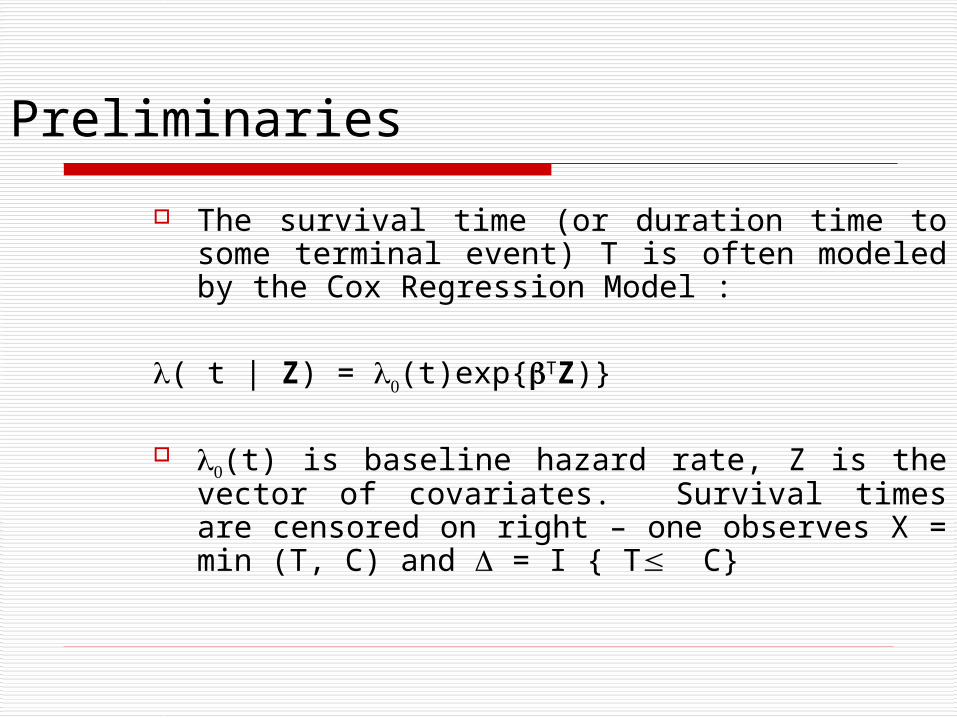
Preliminaries

The survival time (or duration time to some terminal event) T is often modeled by the Cox Regression Model :

( t | Z) = (t)exp{TZ)}

(t) is baseline hazard rate, Z is the vector of covariates. Survival times are censored on right – one observes X = min (T, C) and = I { T C}

Types of Covariates

External – Not directly involved with the failure mechanism

Internal – Generated by the individual under study – observed only as long as the individual survives

Solution to the full model

Parameter vector obtained 0 by maximizing the following:

i

n

1in

1jijij

ii

)X('exp)XX(I

)X('exp)(L

Z

Z

Estimate of the cumulative hazard function:

tX n

jijij

ii

)X('exp)XX(I)t(ˆ

oftimesfailurebetweenerpolationintLinear

1

Z

Goodness of Fit:

Graphical Methods

Chi-Squared Type Tests

Lin’s Method of Weights

Problem – Missing Data

Missing Covariates – often due to drop out

Let denote the history of the covariate upto time t:

Let T be the time to some event. Then thehazard of T at time t is

((t)| )dt = lim dt →0 Pr( t < T < t + dt)| )

)t(Z

)t(Z

)t(Z

CLASSIFICATION OF THE DROP-OUT PROCESS

Completely Random Dropout – Drop-out process is independent of both observed and non observed measurements.

Random Drop-out – Drop-out process is independent of unobserved measurements, but depends on the observed measurements.

Nonignorable Drop-out – Drop-out process depends on unobserved measurements.

Approaches Use only the complete observations

Replace missing values with sample mean.

Estimate missing values with consistent estimators so that the likelihood is maximized (IMPUTATION)

Previous Notable Work for Nonignorable Dropout

Diggle and Kenward (1994) Little (1995), Hogan and Laird (1997) - Essentially one integrates out the

unobserved covariates

Martinussen (1999) – uses EM algorithm

Work of Dupuy and Mesbah

Subjects measured at discrete time intervals

Terminal Event – Disease Progression

Patients can dropout and covariate can be unobserved at dropout

The Model n subjects observed at fixed times tj,

t0 = 0 < . . . < tj-1 < tj< . . . <

0 < 0 t = tj – tj-1 < 1 <

Let Z = internal covariate and Zi(t) = value of Z at time t for the ith individual

Z i, j denote the response for the ith subject on (tj, tj+1].

Hazard Rate

= (t)exp(Tw(t))

where w(t) = (z(t – t), z(t))T

= ()T or = ()T

))t(z|t(

Assumptions 1)      The covariate vector Z is assumed to

have uniformly bounded continuous density f(z,

2)      The censoring time C has continuous distribution function GC(u)

3)      The censoring distribution is assumed to be independent of the unobserved covariate, and of the parameters , and .

Likelihood

dz);z,z.,..,z(fdue)u()x(wexp)x(1x

)u(Tw

a0

x

0

T

L() =

Let us call the above model Equation (1)

Solution

Method of Sieves:

Replace original parameter space of the parameters () by an approximating space n, called the sieve.

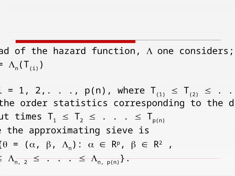
Instead of the hazard function, one considers;

n,i = n(T(i))

T(i), i = 1, 2,. . ., p(n), where T(1) T(2) . . . T(p(n)

are the order statistics corresponding to the distinct

dropout times T1 T2 . . . Tp(n)

Hence the approximating sieve is

n = { = (, , n): Rp, R2 ,

n, 1 n, 2 . . . n, p(n)}.

One maximizes the psuedo-likelihood function:

Ln() = )(Ln

1i

)i(

here L(i) () =

dz) ; z, z .,. ., z( f e ) x( w exp1 i x

i x ) k(

) k( iT

}i x ) k( T i

a,i 0,iT: k

) T( wk, n i i

Ti

) n( p

1 k

1

k, n

dz);z,z.,..,z(fe)x(wexp

1ix

ix)k(

)k(iT

}ix)k(Ti

a,i0,iT:k

)T(wk,nii

Ti

)n(p

1k

1

k,n

THE MLE

)ˆ,ˆ,ˆ(ˆnnnn

The MLE

Obtained via the EM algorithm is identifiable and asymptotically normally distributed

Goodness-of-fit for Dupuy’s Model

Issue of Model Checking Important

PROBLEM – MISSING DATA

Could use DOUBLE SAMPLING or IMPUTATION

SOLUTION: Validate model in Equation (1) – Marginal Model

Done by Using the Weights Method of Lin (1991)

Development of the Test Statistic

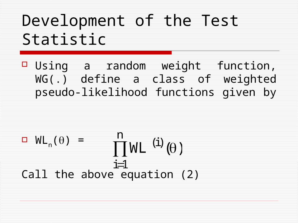
Using a random weight function, WG(.) define a class of weighted pseudo-likelihood functions given by

WLn() =

Call the above equation (2)

)(WLn

1i

)i(

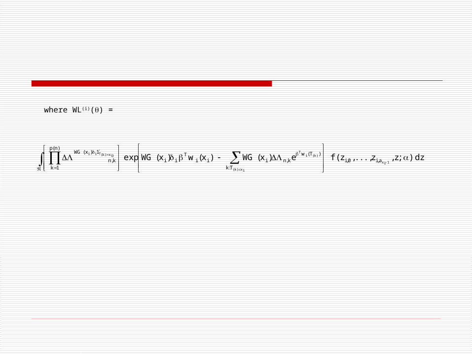
where WL(i)() =

dz);z,z.,..,z(fe)x(WG)x(w)x(WGexp1ix

ix)k(

)k(iT

}ix)k(Tii

a,i0,i

T:k

)T(wk,niii

Tii

)n(p

1k

1)x(WG

k,n

Define the maximizer of equation (2) as:

)ˆ,ˆ,ˆ(ˆn,Wn,Wn,Wn,W

The test statistic is a function of n,W

Asymptotic Results For

Under the model in Equation (1), the vector converges in

distribution to a bivariate normal

distribution with zero mean and a covariance matrix

n,W

)ˆ(n 0n,W

10,W

X

00

)u(WT )u(de)u(W)u(W)X(WGET0

0

0,WHere

If model in Equation (1) is correct, the weighted and the nonweighted MLE’s should be close to each other:

Under the model in Eqn (1), the vector converges in distribution to a bivariate normal distribution with zero mean and a covariance matrix DW =

)ˆˆ(n nn,W

10

10,W

X

00

)u(WT0 )u(de)u(W)u(WE

T0

0

Note that

Proof still in progress

Proposed method:

Show that score function for weighted likelihood and unweighted likelihood are asymptotically joint normal.

Use counting process techniques and martingale theory.

THE TEST STATISTIC

)ˆˆ(D)ˆˆ(nQ nn,W1

WT

nn,WW

Under the model in Equation (1), the above statistic will have a chi-square distribution with 2 degrees of freedom.