Goodness of Fit - University of Arizonamath.arizona.edu/~jwatkins/U_gof.pdf · Goodness of Fit 21.1 Fit of a ... the likelihood ratio test will have a chi-square test statistic with

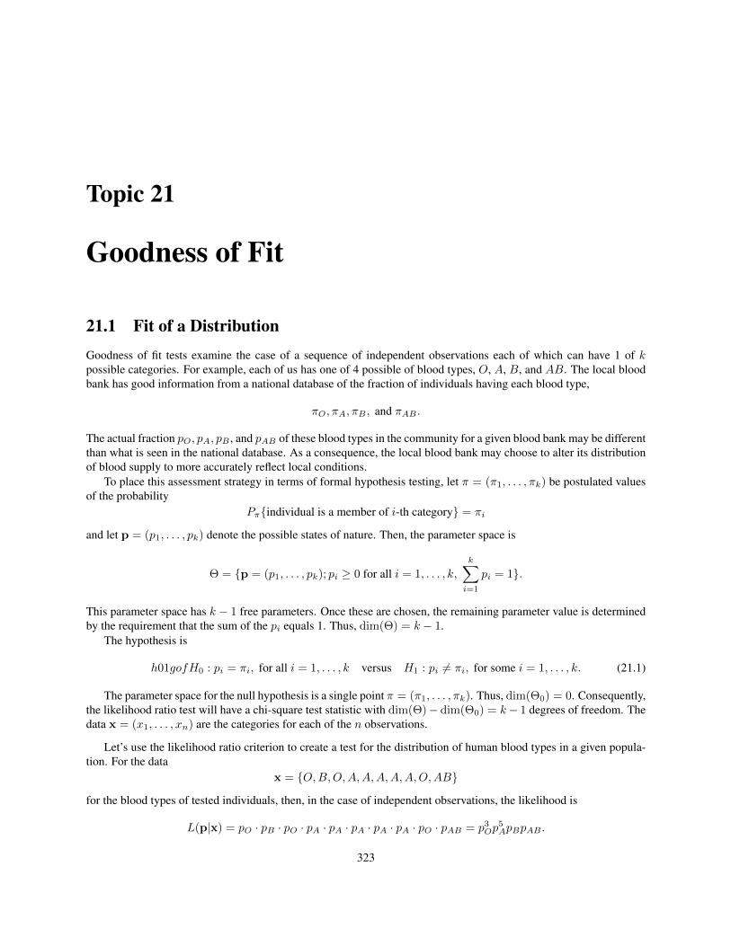
Topic 21

Goodness of Fit

21.1 Fit of a DistributionGoodness of fit tests examine the case of a sequence of independent observations each of which can have 1 of kpossible categories. For example, each of us has one of 4 possible of blood types, O, A, B, and AB. The local bloodbank has good information from a national database of the fraction of individuals having each blood type,

⇡O,⇡A,⇡B , and ⇡AB .

The actual fraction pO, pA, pB , and pAB of these blood types in the community for a given blood bank may be differentthan what is seen in the national database. As a consequence, the local blood bank may choose to alter its distributionof blood supply to more accurately reflect local conditions.

To place this assessment strategy in terms of formal hypothesis testing, let ⇡ = (⇡1

, . . . ,⇡k) be postulated valuesof the probability

P⇡{individual is a member of i-th category} = ⇡i

and let p = (p1

, . . . , pk) denote the possible states of nature. Then, the parameter space is

⇥ = {p = (p1

, . . . , pk); pi � 0 for all i = 1, . . . , k,k

X

i=1

pi = 1}.

This parameter space has k � 1 free parameters. Once these are chosen, the remaining parameter value is determinedby the requirement that the sum of the pi equals 1. Thus, dim(⇥) = k � 1.

The hypothesis is

h01gofH0

: pi = ⇡i, for all i = 1, . . . , k versus H1

: pi 6= ⇡i, for some i = 1, . . . , k. (21.1)

The parameter space for the null hypothesis is a single point ⇡ = (⇡1

, . . . ,⇡k). Thus, dim(⇥

0

) = 0. Consequently,the likelihood ratio test will have a chi-square test statistic with dim(⇥)� dim(⇥

0

) = k� 1 degrees of freedom. Thedata x = (x

1

, . . . , xn) are the categories for each of the n observations.

Let’s use the likelihood ratio criterion to create a test for the distribution of human blood types in a given popula-tion. For the data

x = {O,B,O,A,A,A,A,A,O,AB}

for the blood types of tested individuals, then, in the case of independent observations, the likelihood is

L(p|x) = pO · pB · pO · pA · pA · pA · pA · pA · pO · pAB = p3Op5

ApBpAB .

323

Introduction to the Science of Statistics Goodness of Fit

Notice that the likelihood has a factor of pi whenever an observation take on the value i. In other words, if wesummarize the data using

ni = #{observations from category i}

to create n = (n1

, n2

, · · · , nk), a vector that records the number of observations in each category, then, the likelihoodfunction

L(p|n) = pn11

· · · pnk

k . (21.2)

The likelihood ratio is the ratio of the maximum value of the likelihood under the null hypothesis and the maxi-mum likelihood for any parameter value. In this case, the numerator is the likelihood evaluated at ⇡.

⇤(n) =L(⇡|n)L(p̂|n) =

⇡n11

⇡n22

· · ·⇡nk

k

p̂n11

p̂n22

· · · p̂nk

k

=

✓

⇡1

p̂1

◆n1

· · ·✓

⇡k

p̂k

◆nk

. (21.3)

To find the maximum likelihood estimator p̂, we, as usual, begin by taking the logarithm in (21.2),

lnL(p|n) =k

X

i=1

ni ln pi.

Because not every set of values for pi is admissible, we cannot just take derivatives, set them equal to 0 and solve.Indeed, we must find a maximum under the constraint

s(p) =k

X

i=1

pi = 1.

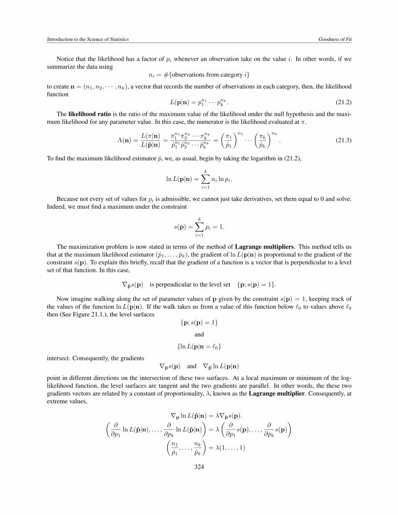
The maximization problem is now stated in terms of the method of Lagrange multipliers. This method tells usthat at the maximum likelihood estimator (p̂

1

, . . . , p̂k), the gradient of lnL(p|n) is proportional to the gradient of theconstraint s(p). To explain this briefly, recall that the gradient of a function is a vector that is perpendicular to a levelset of that function. In this case,

rp̂

s(p) is perpendicular to the level set {p; s(p) = 1}.

Now imagine walking along the set of parameter values of p given by the constraint s(p) = 1, keeping track ofthe values of the function lnL(p|n). If the walk takes us from a value of this function below `

0

to values above `0

then (See Figure 21.1.), the level surfaces{p; s(p) = 1}

and

{lnL(p|n = `0

}

intersect. Consequently, the gradientsr

p̂

s(p) and rp̂

lnL(p|n)

point in different directions on the intersection of these two surfaces. At a local maximum or minimum of the log-likelihood function, the level surfaces are tangent and the two gradients are parallel. In other words, the these twogradients vectors are related by a constant of proportionality, �, known as the Lagrange multiplier. Consequently, atextreme values,

rp

lnL(p̂|n) = �rp̂

s(p).✓

@

@p1

lnL(p̂|n), . . . , @

@pklnL(p̂|n)

◆

= �

✓

@

@p1

s(p), . . . ,@

@pks(p)

◆

✓

n1

p̂1

, . . . ,nk

p̂k

◆

= �(1, . . . , 1)

324


s(p) = 1

OHvel sets for the ORJ�OLNHOLKRRG, values increasingmoving GRZQward

−−

Figure 21.1: Lagrange multipliers Level sets of the log-likelihood function.shown in dashed blue. The level set {s(p) = 1} shown in black. Thegradients for the log-likelihood function and the constraint are indicated by dashed blue and black arrows, respectively. At the maximum, these twoarrows are parallel. Their ratio � is called the Lagrange multiplier. If we view the blue dashed lines as elevation contour lines and the black line asa trail, crossing contour line indicates walking either up or down hill. When the trail reaches its highest elevation, the trail is tangent to a contourline and the gradient for the hill is perpendicular to the trail.

Each of the components of the two vectors must be equal. In other words,

ni

p̂i= �, ni = �p̂i for all i = 1, . . . , k. (21.4)

Now sum this equality for all values of i and use the constraint s(p) = 1 to obtain

n =

kX

i=1

ni = �k

X

i=1

p̂i = �s(ˆp) = �.

Returning to (21.4), we have thatn1

p̂i= n and p̂i =

ni

n.

This is the answer we would guess - the estimate for pi is the fraction of observations in category i. Thus, for theintroductory example,

p̂O =

3

10

, p̂A =

5

10

, p̂B =

1

10

, and p̂O =

1

10

.

Next, we substitute the maximum likelihood estimates p̂i = ni/n into the likelihood ratio (21.3) to obtain

⇤(n) =L(⇡|n)L(p̂|n) =

✓

⇡1

n1

/n

◆n1

· · ·✓

⇡k

nk/n

◆nk

=

✓

n⇡1

n1

◆n1

· · ·✓

n⇡k

nk

◆nk

. (21.5)

Recall that we reject the null hypothesis if this ratio is too low, i.e, the maximum likelihood under the null hypoth-esis is sufficiently smaller than the maximum likelihood under the alternative hypothesis.

Let’s review the process. the random variables X1

, X2

, . . . , Xn are independent, taking values in one of k cate-gories each having distribution ⇡. In the example, we have 4 categories, namely the common blood types O, A, B,and AB. Next, we organize the data into

Ni = #{j;Xj = i},

325


the number of observations in category i. Next, create the vector N = (N1

, . . . , Nk) to be the vector of observednumber of occurrences for each category i. In the example we have the vector (3,5,1,1) for the number of occurrencesof the 4 blood types.

When the null hypothesis holds true, �2 ln⇤(N) has approximately a �2

k�1

distribution. Using (21.5) we obtainthe the likelihood ratio test statistic

�2 ln⇤(N) = �2

kX

i=1

Ni lnn⇡i

Ni= 2

kX

i=1

Ni lnNi

n⇡i

The last equality uses the identity ln(1/x) = � lnx for the logarithm of reciprocals.The test statistic �2 ln⇤n(n) is generally rewritten using the notation Oi = ni for the number of observed

occurrences of i and Ei = n⇡i for the number of expected occurrences of i as given by H0

. Then, we can write thetest statistic as

�2 ln⇤n(O) = 2

kX

i=1

Oi lnOi

Ei(21.6)

This is called the G2 test statistic. Thus, we can perform our inference on the hypothesis (??) by evaluating G2. Thep-value will be the probability that the a �2

k�1

random variable takes a value greater than �2 ln⇤n(O)

The traditional method for a test of goodness of fit, we use, instead of the G2 statistic, the chi-square statistic

�2

=

kX

i=1

(Ei �Oi)2

Ei. (21.7)

This was introduced between 1895 and 1900 by Karl Pearson and consequently has been in use for longer that theconcept of likelihood ratio tests. We establish the relation between (21.6) and (21.7), through the following twoexercises.

Exercise 21.1. Define

�i =Oi � Ei

Ei=

Oi

Ei� 1.

Show thatk

X

i=1

Ei�i = 0 and Ei(1 + �i) = Oi.

Exercise 21.2. Show the relationship between the G2 and �2 statistics in (21.6) and (21.7) by applying the quadraticTaylor polynomial approximation for the natural logarithm,

ln(1 + �i) ⇡ �i �1

2

�2i

and keeping terms up to the square of �i

To compute either the G2 or �2 statistic, we begin by creating a table.

i 1 2 · · · kobserved O

1

O2

· · · Ok

expected E1

E2

· · · Ek

We show this procedure using a larger data set on blood types.

326


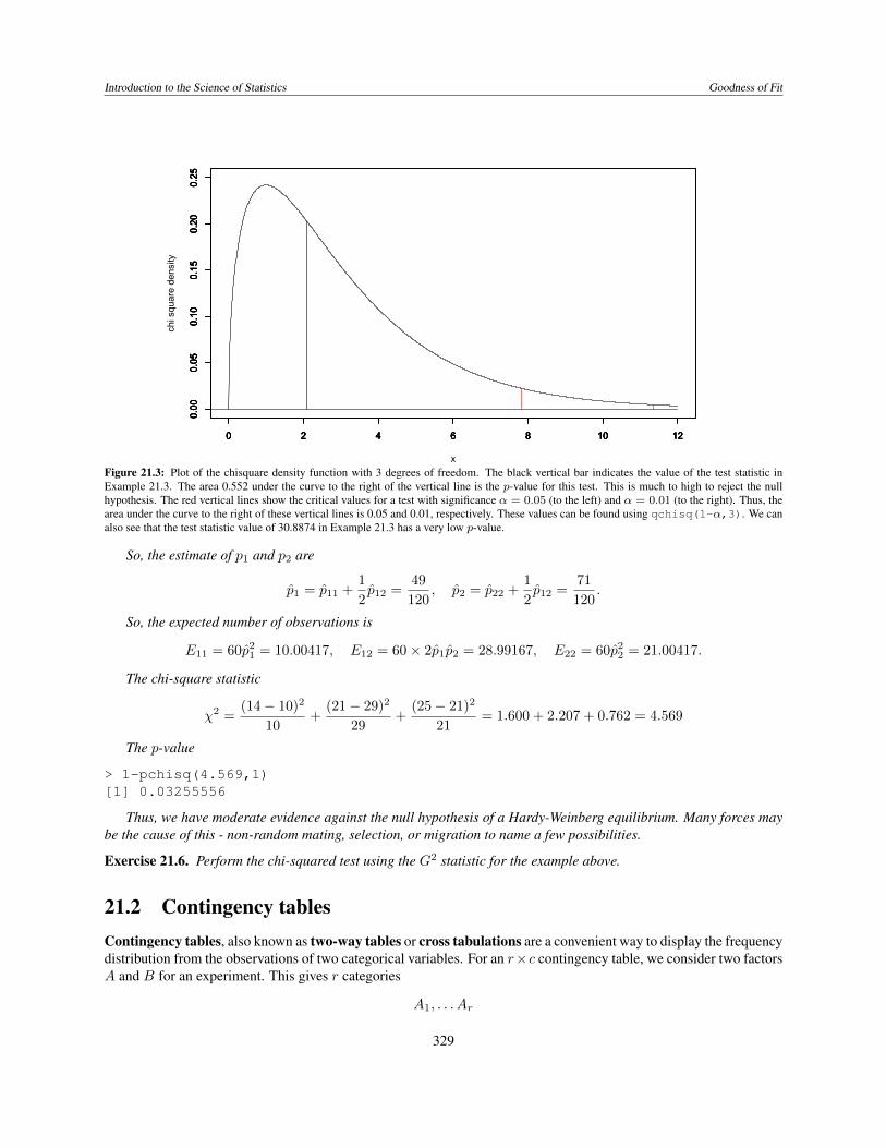
Example 21.3. The Red Cross recommends that a blood bank maintains 44% blood type O, 42% blood type A, 10%blood type B, 4% blood type AB. You suspect that the distribution of blood types in Tucson is not the same as therecommendation. In this case, the hypothesis is

H0

: pO = 0.44, pA = 0.42, pB = 0.10, pAB = 0.04 versus H1

: at least one pi is unequal to the given values

Based on 400 observations, we observe 228 for type O, 124 for type A, 40 for type B and 8 for type AB bycomputing 400⇥ pi using the values in H

0

. This gives the table

type O A B ABobserved 228 124 40 8expected 176 168 40 16

Using this table, we can compute the value of either (21.6) and (21.7). The chisq.test command in R uses(21.7). The program computes the expected number of observations.

> chisq.test(c(228,124,40,8),p=c(0.44,0.42,0.10,0.04))

Chi-squared test for given probabilities

data: c(228, 124, 40, 8)X-squared = 30.8874, df = 3, p-value = 8.977e-07

The number of degrees of freedom is 4� 1 = 3. Note that the p-value is very low and so the distribution of bloodtypes in Tucson is very unlikely to be the same as the national distribution.

We can also perform the test using the G2-statistic in (21.6):

> O<-c(228,124,40,8)> E<-sum(O)*c(0.44,0.42,0.10,0.04)> G2stat<-2*sum(O*log(O/E))> G2stat[1] 31.63731> 1-pchisq(G2stat,3)[1] 6.240417e-07

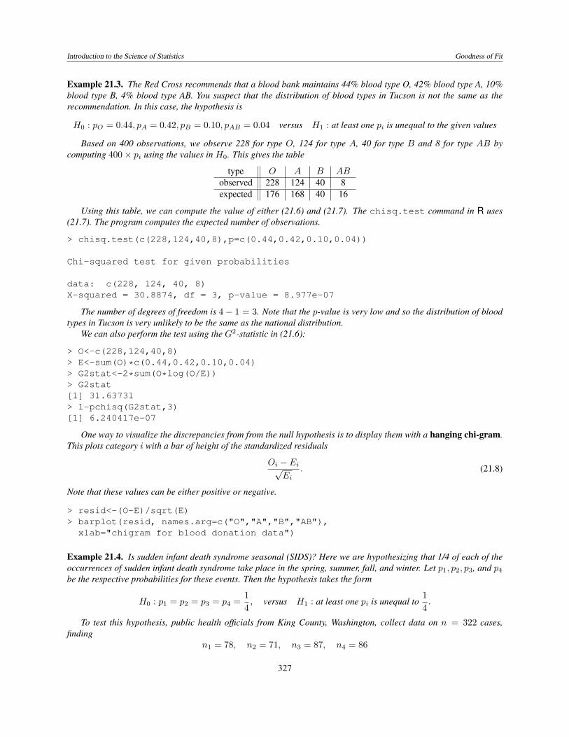
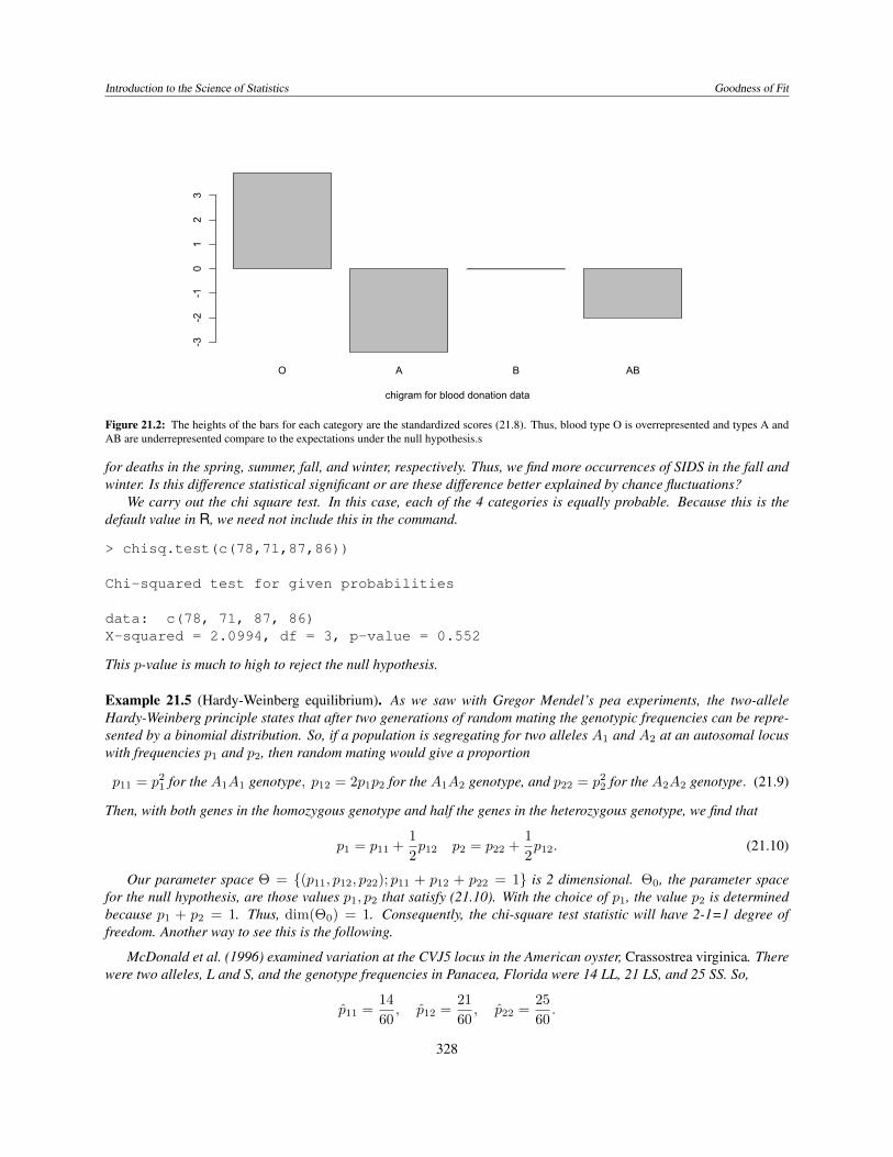
One way to visualize the discrepancies from from the null hypothesis is to display them with a hanging chi-gram.This plots category i with a bar of height of the standardized residuals

Oi � EipEi

. (21.8)

Note that these values can be either positive or negative.

> resid<-(O-E)/sqrt(E)> barplot(resid, names.arg=c("O","A","B","AB"),

xlab="chigram for blood donation data")

Example 21.4. Is sudden infant death syndrome seasonal (SIDS)? Here we are hypothesizing that 1/4 of each of theoccurrences of sudden infant death syndrome take place in the spring, summer, fall, and winter. Let p

1

, p2

, p3

, and p4

be the respective probabilities for these events. Then the hypothesis takes the form

H0

: p1

= p2

= p3

= p4

=

1

4

, versus H1

: at least one pi is unequal to1

4

.

To test this hypothesis, public health officials from King County, Washington, collect data on n = 322 cases,finding

n1

= 78, n2

= 71, n3

= 87, n4

= 86

327


O A B AB

chigram for blood donation data

-3-2

-10

12

3

Figure 21.2: The heights of the bars for each category are the standardized scores (21.8). Thus, blood type O is overrepresented and types A andAB are underrepresented compare to the expectations under the null hypothesis.s

for deaths in the spring, summer, fall, and winter, respectively. Thus, we find more occurrences of SIDS in the fall andwinter. Is this difference statistical significant or are these difference better explained by chance fluctuations?

We carry out the chi square test. In this case, each of the 4 categories is equally probable. Because this is thedefault value in R, we need not include this in the command.

> chisq.test(c(78,71,87,86))

Chi-squared test for given probabilities

data: c(78, 71, 87, 86)X-squared = 2.0994, df = 3, p-value = 0.552

This p-value is much to high to reject the null hypothesis.

Example 21.5 (Hardy-Weinberg equilibrium). As we saw with Gregor Mendel’s pea experiments, the two-alleleHardy-Weinberg principle states that after two generations of random mating the genotypic frequencies can be repre-sented by a binomial distribution. So, if a population is segregating for two alleles A

1

and A2

at an autosomal locuswith frequencies p

1

and p2

, then random mating would give a proportion

p11

= p21

for the A1

A1

genotype, p12

= 2p1

p2

for the A1

A2

genotype, and p22

= p22

for the A2

A2

genotype. (21.9)

Then, with both genes in the homozygous genotype and half the genes in the heterozygous genotype, we find that

p1

= p11

+

1

2

p12

p2

= p22

+

1

2

p12

. (21.10)

Our parameter space ⇥ = {(p11

, p12

, p22

); p11

+ p12

+ p22

= 1} is 2 dimensional. ⇥

0

, the parameter spacefor the null hypothesis, are those values p

1

, p2

that satisfy (21.10). With the choice of p1

, the value p2

is determinedbecause p

1

+ p2

= 1. Thus, dim(⇥

0

) = 1. Consequently, the chi-square test statistic will have 2-1=1 degree offreedom. Another way to see this is the following.

McDonald et al. (1996) examined variation at the CVJ5 locus in the American oyster, Crassostrea virginica. Therewere two alleles, L and S, and the genotype frequencies in Panacea, Florida were 14 LL, 21 LS, and 25 SS. So,

p̂11

=

14

60

, p̂12

=

21

60

, p̂22

=

25

60

.

328


0 2 4 6 8 10 12

0.00

0.05

0.10

0.15

0.20

0.25

x

chi square

den

sity

0 2 4 6 8 10 12

0.00

0.05

0.10

0.15

0.20

0.25

0 2 4 6 8 10 12

0.00

0.05

0.10

0.15

0.20

0.25

0 2 4 6 8 10 12

0.00

0.05

0.10

0.15

0.20

0.25

0 2 4 6 8 10 12

0.00

0.05

0.10

0.15

0.20

0.25

Figure 21.3: Plot of the chisquare density function with 3 degrees of freedom. The black vertical bar indicates the value of the test statistic inExample 21.3. The area 0.552 under the curve to the right of the vertical line is the p-value for this test. This is much to high to reject the nullhypothesis. The red vertical lines show the critical values for a test with significance ↵ = 0.05 (to the left) and ↵ = 0.01 (to the right). Thus, thearea under the curve to the right of these vertical lines is 0.05 and 0.01, respectively. These values can be found using qchisq(1-↵,3). We canalso see that the test statistic value of 30.8874 in Example 21.3 has a very low p-value.

So, the estimate of p1

and p2

are

p̂1

= p̂11

+

1

2

p̂12

=

49

120

, p̂2

= p̂22

+

1

2

p̂12

=

71

120

.

So, the expected number of observations is

E11

= 60p̂21

= 10.00417, E12

= 60⇥ 2p̂1

p̂2

= 28.99167, E22

= 60p̂22

= 21.00417.

The chi-square statistic

�2

=

(14� 10)

2

10

+

(21� 29)

2

29

+

(25� 21)

2

21

= 1.600 + 2.207 + 0.762 = 4.569

The p-value

> 1-pchisq(4.569,1)[1] 0.03255556

Thus, we have moderate evidence against the null hypothesis of a Hardy-Weinberg equilibrium. Many forces maybe the cause of this - non-random mating, selection, or migration to name a few possibilities.

Exercise 21.6. Perform the chi-squared test using the G2 statistic for the example above.

21.2 Contingency tablesContingency tables, also known as two-way tables or cross tabulations are a convenient way to display the frequencydistribution from the observations of two categorical variables. For an r⇥c contingency table, we consider two factorsA and B for an experiment. This gives r categories

A1

, . . . Ar

329


for factor A and c categoriesB

1

, . . . Bc

for factor B.Here, we write Oij to denote the number of occurrences for which an individual falls into both category Ai and

category Bj . The results is then organized into a two-way table.

B1

B2

· · · Bc totalA

1

O11

O12

· · · O1c O

1·A

2

O21

O22

· · · O2c O

2·...

......

. . ....

...Ar Or1 Or2 · · · Orc Or·

total O·1 O·2 · · · O·c n

Example 21.7. Returning to the study of the smoking habits of 5375 high school children in Tucson in 1967, here is atwo-way table summarizing some of the results.

student studentsmokes does not smoke total

2 parents smoke 400 1380 17801 parent smokes 416 1823 22390 parents smoke 188 1168 1356

total 1004 4371 5375

For a contingency table, the null hypothesis we shall consider is that the factors A and B are independent. To setthe parameters for this model, we define

pij = P{an individual is simultaneously a member of category Ai and category Bj}.

Then, we have the parameter space

⇥ = {p = (pij , 1 i r, 1 j c); pij � 0 for all i, j = 1,r

X

i=1

cX

j=1

pij = 1}.

Write the marginal distribution

pi· =c

X

j=1

pij = P{an individual is a member of category Ai}

and

p·j =r

X

i=1

pij = P{an individual is a member of category Bj}.

The null hypothesis of independence of the categories A and B can be written

H0

: pij = pi·p·j , for all i, j versus H1

: pij 6= pi·p·j , for some i, j.

Follow the procedure as before for the goodness of fit test to end with a G2 and its corresponding �2 test statistic.The G2 statistic follows from the likelihood ratio test criterion. The �2 statistics is a second order Taylor seriesapproximation to G2.

�2

rX

i=1

cX

j=1

Oij lnEij

Oij⇡

rX

i=1

cX

j=1

(Oij � Eij)2

Eij.

330


The null hypothesis pij = pi·p·j can be written in terms of observed and expected observations as

Eij

n=

Oi·n

O·jn

.

orEij =

Oi·O·jn

.

The test statistic, under the null hypothesis, has a �2 distribution. To determine the number of degrees of freedom,consider the following. Start with a contingency table with no entries but with the prescribed marginal values.

B1

B2

· · · Bc totalA

1

O1·

A2

O2·

......

Ar Or·total O·1 O·2 · · · O·c n

The number of degrees of freedom is the number of values that we can place in the contingency table before all theremaining values are determined. To begin, fill in the first row with values E

11

, E12

, . . . , E1,c�1

. The final value E1,c

in this determined by the other values in the row and the constraint that the row sum must be O1·. Continue filling the

rows, noting that the value in column c is determined by the constraint on the row sum. Finally, when the time comesto fill in the bottom row r, notice that all the values are determined by the constraint on the row sums O·j . Thus, wecan fill c�1 values in each of the r�1 rows before the remaining values are determined. Thus, the number of degreesof freedom is (r � 1)⇥ (c� 1),

Example 21.8. Returning to the data set on smoking habits in Tucson, we find that the expected table is

student studentsmokes does not smoke total

2 parents smoke 332.49 1447.51 17801 parent smokes 418.22 1820.78 22390 parents smoke 253.29 1102.71 1356

total 1004 4371 5375

For example,

E11

=

O1·O·1n

=

1780 · 10045375

= 332.49.

To compute the chi-square statistic

(400�332.49)2

332.49 +

(1380�1447.51)2

1447.51

+

(416�418.22)2

418.22 +

(1823�1820.78)2

1820.78

+

(188�253.29)2

253.29 +

(1168�1102.71)2

1102.71

= 13.71 + 3.15

+ 0.012 + 0.003

+ 16.83 + 3.866

= 37.57

331


The number of degrees of freedom is (r � 1)⇥ (c� 1) = (3� 1)⇥ (2� 1) = 2. This can be seen by noting thatone the first two entries in the ”student smokes” column is filled, the rest are determined. Thus, the p-value

> 1-pchisq(37.57,2)[1] 6.946694e-09

is very small and leads us to reject the null hypothesis. Thus, we conclude that children smoking habits are notindependent of their parents smoking habits. An examination of the individual cells shows that the children of parentswho do not smoke are less likely to smoke and children who have two parents that smoke are more likely to smoke.Under the null hypothesis, each cell has a mean approximately 1 and so values much greater than 1 show contributionthat leads to the rejection of H

0

.R does the computation for us using the chisq.test command

> smoking<-matrix(c(400,416,188,1380,1823,1168),nrow=3)> smoking

[,1] [,2][1,] 400 1380[2,] 416 1823[3,] 188 1168> chisq.test(smoking)

Pearson’s Chi-squared test

data: smokingX-squared = 37.5663, df = 2, p-value = 6.959e-09

We can look at the residuals (Oij � Eij)/p

Eij for the entries in the �2 test as follows.

> smokingtest<-chisq.test(smoking)> residuals(smokingtest)

[,1] [,2][1,] 3.7025160 -1.77448934[2,] -0.1087684 0.05212898[3,] -4.1022973 1.96609088

Notice that if we square these values, we obtain the entries found in computing the test statistic.

> residuals(smokingtest)ˆ2[,1] [,2]

[1,] 13.70862455 3.14881241[2,] 0.01183057 0.00271743[3,] 16.82884348 3.86551335

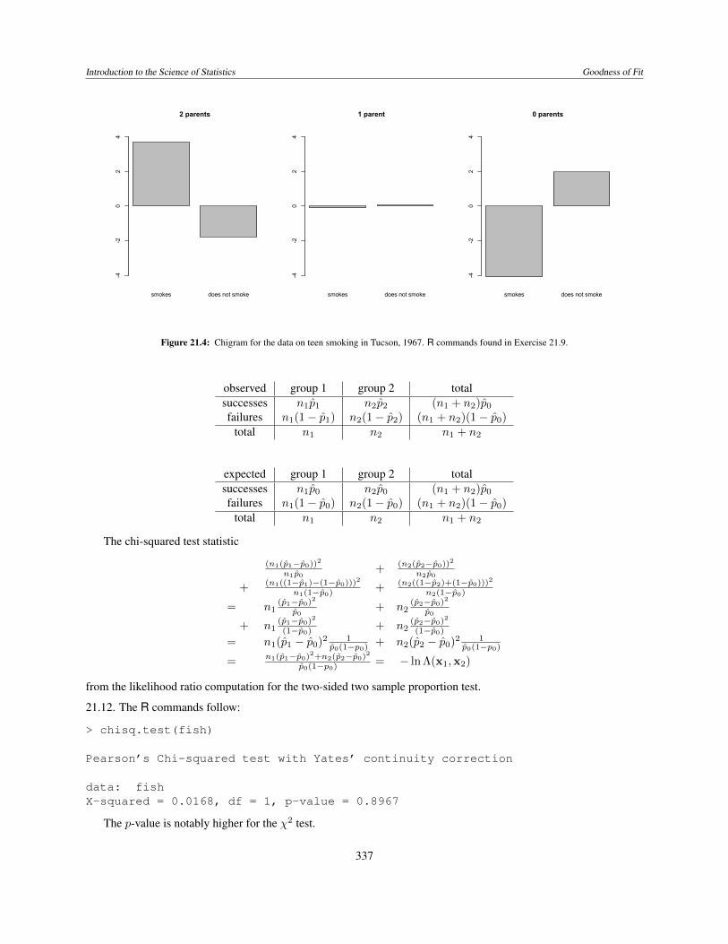
Exercise 21.9. Make three horizontally placed chigrams that summarize the residuals for this �2 test in the exampleabove.

Exercise 21.10 (two-by-two tables). Here is the contingency table can be thought of as two sets of Bernoulli trials asshown.

group 1 group 2 totalsuccesses x

1

x2

x1

+ x2

failures n1

� x1

n2

� x2

(n1

+ n2

)� (x1

+ x2

)

total n1

n2

n1

+ n2

Show that the chi-square test is equivalent to the two-sided two sample proportion test.

332


21.3 Applicability and Alternatives to Chi-squared TestsThe chi-square test uses the central limit theorem and so is based on the ability to use a normal approximation. Onecriterion, the Cochran conditions requires no cell has count zero, and more than 80% of the cells have counts at least5. If this does not hold, then Fisher’s exact test uses the hypergeometric distribution (or its generalization) directlyrather than normal approximation.

For example, for the 2⇥ 2 table,

B1

B2

totalA

1

O11

O12

O1·

A2

O21

O22

O2·

total O·1 O·2 n

The idea behind Fisher’s exact test is to begin with an empty table:

B1

B2

totalA

1

O1·

A2

O2·

total O·1 O·2 n

and a null hypothesis that uses equally likely outcomes to fill in the table. We will use as an analogy the model ofmark and recapture. Normally the goal is to find n, the total population. In this case, we assume that this populationsize is known and will consider the case that the individuals in the two captures are independent. This is assumed inthe mark and recapture protocol. Here we test this independence.

In this regard,

• A1

- an individual in the first capture and thus tagged.

• A2

- an individual not in the first capture and thus not tagged.

• B1

- an individual in the second capture.

• B2

- an individual not in the second capture

Then, from the point of view of the A classification:

• We have O1· from a population n with the A

1

classification (tagged individuals). This can be accomplished in✓

n

O1·

◆

=

n!

O1·!O2·!

ways. The remaining O2· = n � O

1· have the A2

classification (untagged individuals). Next, we fill in thevalues for the B classification

• From the O·1 belonging to category B1

(individuals in the second capture), O11

also belong to A1

(have a tag).This outcome can be accomplished in

✓

O·1O

11

◆

=

O·1!

O11

!O21

!

ways.

• From the O·2 belonging to category B2

(individuals not in the second capture), O12

also belong to A1

(have atag). This outcome can be accomplished in

✓

O·2O

21

◆

=

O·2!

O12

!O22

!

ways.

333


Under the null hypothesis that every individual can be placed in any group, provided we have the given marginalinformation. In this case, the probability of the table above has the formula from the hypergeometric distribution

�O1·O11

��O2··O21

�

� nO·1

�

=

O·1!/(O11

!O21

!) ·O·2!/(O12

!O22

!)

n!/(O1·!O2·!)

=

O·1!O·2!O1·!O2·!

O11

!O12

!O21

!O22

!n!. (21.11)

Notice that the formula is symmetric in the column and row variables. Thus, if we had derived the hypergeometricformula from the point of view of the B classification we would have obtained exactly the same formula (21.11).

To complete the exact test, we rely on statistical software to do the following:

• compute the hypergeometric probabilities over all possible choices for entries in the cells that result in the givenmarginal values, and

• rank these probabilities from most likely to least likely.

• Find the ranking of the actual data.

• For a one-sided test of too rare, the p-value is the sum of probabilities of the ranking lower than that of the data.

A similar procedure applies to provide the Fisher exact test for r ⇥ c tables.

Example 21.11. As a test of the assumptions for mark and recapture. We examine a small population of 120 fish. Theassumption are that each group of fish are equally likely to be capture in the first and second capture and that the twocaptures are independent. This could be violated, for example, if the tagged fish are not uniformly dispersed in thepond.

Twenty-five are tagged and returned to the pond. For the second capture of 30, seven are tagged. With thisinformation, given in red in the table below, we can complete the remaining entries.

in 2nd capture not in 2nd capture totalin 1st capture 7 18 25

not in 1st capture 23 72 95total 30 90 120

Fisher’s exact test show a much too high p-value to reject the null hypothesis.

> fish<-matrix(c(7,23,18,72),ncol=2)> fisher.test(fish)

Fisher’s Exact Test for Count Data

data: fishp-value = 0.7958alternative hypothesis: true odds ratio is not equal to 195 percent confidence interval:0.3798574 3.5489546

sample estimates:odds ratio

1.215303

Exercise 21.12. Perform the �2 test on the data set above and report the findings.

Example 21.13. We now return to a table on hemoglobin genotypes on two Indonesian islands. Recall that heterozy-gotes are protected against malaria.

334


genotype AA AE EEFlores 128 6 0Sumba 119 78 4

We noted that heterozygotes are rare on Flores and that it appears that malaria is less prevalent there since theheterozygote does not provide an adaptive advantage. Here are both the chi-square test and the Fisher exact test.

> genotype<-matrix(c(128,119,6,78,0,4),nrow=2)> genotype

[,1] [,2] [,3][1,] 128 6 0[2,] 119 78 4> chisq.test(genotype)

Pearson’s Chi-squared test

data: genotypeX-squared = 54.8356, df = 2, p-value = 1.238e-12

Warning message:In chisq.test(genotype) : Chi-squared approximation may be incorrect

and

> fisher.test(genotype)

Fisher’s Exact Test for Count Data

data: genotypep-value = 3.907e-15alternative hypothesis: two.sided

Note that R cautions against the use of the chi-square test with these data.

21.4 Answer to Selected Exercise21.1. For the first identity, using �i = (Oi � Ei)/Ei.

kX

i=1

Ei�i =k

X

i=1

EiOi � Ei

Ei=

kX

i=1

(Oi � Ei) = n� n = 0

and for the second

Ei(1 + �i) = Ei

✓

Ei

Ei+

Oi � Ei

Ei

◆

= EiOi

Ei= Oi.

21.2. We apply the quadratic Taylor polynomial approximation for the natural logarithm,

ln(1 + �i) ⇡ �i �1

2

�2i ,

335


and use the identities in the previous exercise. Keeping terms up to the square of �i, we find that

�2 ln⇤n(O) = 2

kX

i=1

Oi lnOi

Ei= 2

kX

i=1

Ei(1 + �i) ln(1 + �i)

⇡ 2

kX

i=1

Ei(1 + �i)(�i �1

2

�2i ) ⇡ 2

kX

i=1

Ei(�i +1

2

�2i )

= 2

kX

i=1

Ei�i +k

X

i=1

Ei�2

i

= 0 +

kX

i=1

(Ei �Oi)2

Ei.

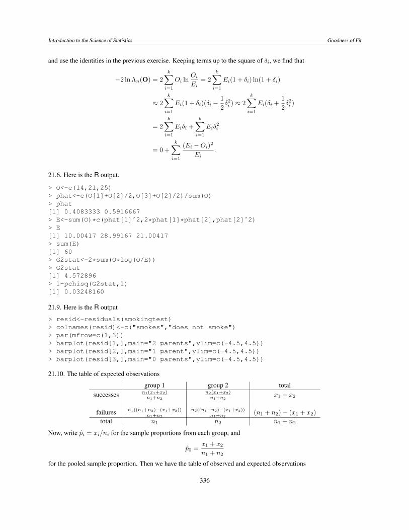
21.6. Here is the R output.

> O<-c(14,21,25)> phat<-c(O[1]+O[2]/2,O[3]+O[2]/2)/sum(O)> phat[1] 0.4083333 0.5916667> E<-sum(O)*c(phat[1]ˆ2,2*phat[1]*phat[2],phat[2]ˆ2)> E[1] 10.00417 28.99167 21.00417> sum(E)[1] 60> G2stat<-2*sum(O*log(O/E))> G2stat[1] 4.572896> 1-pchisq(G2stat,1)[1] 0.03248160

21.9. Here is the R output

> resid<-residuals(smokingtest)> colnames(resid)<-c("smokes","does not smoke")> par(mfrow=c(1,3))> barplot(resid[1,],main="2 parents",ylim=c(-4.5,4.5))> barplot(resid[2,],main="1 parent",ylim=c(-4.5,4.5))> barplot(resid[3,],main="0 parents",ylim=c(-4.5,4.5))

21.10. The table of expected observations

group 1 group 2 totalsuccesses n1(x1+x2)

n1+n2

n2(x1+x2)

n1+n2x1

+ x2

failures n1((n1+n2)�(x1+x2))

n1+n2

n2((n1+n2)�(x1+x2))

n1+n2(n

1

+ n2

)� (x1

+ x2

)

total n1

n2

n1

+ n2

Now, write p̂i = xi/ni for the sample proportions from each group, and

p̂0

=

x1

+ x2

n1

+ n2

for the pooled sample proportion. Then we have the table of observed and expected observations

336


smokes does not smoke

2 parents-4

-20

24

smokes does not smoke

1 parent

-4-2

02

4smokes does not smoke

0 parents

-4-2

02

4

Figure 21.4: Chigram for the data on teen smoking in Tucson, 1967. R commands found in Exercise 21.9.

observed group 1 group 2 totalsuccesses n

1

p̂1

n2

p̂2

(n1

+ n2

)p̂0

failures n1

(1� p̂1

) n2

(1� p̂2

) (n1

+ n2

)(1� p̂0

)

total n1

n2

n1

+ n2

expected group 1 group 2 totalsuccesses n

1

p̂0

n2

p̂0

(n1

+ n2

)p̂0

failures n1

(1� p̂0

) n2

(1� p̂0

) (n1

+ n2

)(1� p̂0

)

total n1

n2

n1

+ n2

The chi-squared test statistic

(n1(p̂1�p̂0))2

n1p̂0+

(n2(p̂2�p̂0))2

n2p̂0

+

(n1((1�p̂1)�(1�p̂0)))2

n1(1�p̂0)+

(n2((1�p̂2)+(1�p̂0)))2

n2(1�p̂0)

= n1

(p̂1�p̂0)2

p̂0+ n

2

(p̂2�p̂0)2

p̂0

+ n1

(p̂1�p̂0)2

(1�p̂0)+ n

2

(p̂2�p̂0)2

(1�p̂0)

= n1

(p̂1

� p̂0

)

2

1

p̂0(1�p0)+ n

2

(p̂2

� p̂0

)

2

1

p̂0(1�p0)

=

n1(p̂1�p̂0)2+n2(p̂2�p̂0)

2

p̂0(1�p0)= � ln⇤(x

1

,x2

)

from the likelihood ratio computation for the two-sided two sample proportion test.

21.12. The R commands follow:

> chisq.test(fish)

Pearson’s Chi-squared test with Yates’ continuity correction

data: fishX-squared = 0.0168, df = 1, p-value = 0.8967

The p-value is notably higher for the �2 test.

337

Documents

Goodness of Fit - University of Arizonamath.arizona.edu/~jwatkins/U_gof.pdf · Goodness of Fit 21.1 Fit of a ... the likelihood ratio test will have a chi-square test statistic with