Government spending and retail prices: Regional evidence from the United States

Rasmus Bisgaard Larsen

rbl@nationalbanken.dk

DANMARKS NATIONALBANK

The Working Papers of Danmarks Nationalbank describe research and development, often still ongoing, as a contribution to the professional debate.

The viewpoints and conclusions stated are the responsibility of the individual contributors, and do not necessarily reflect the views of Danmarks Nationalbank.

8 S E P T E M B ER 20 21 — NO . 18 1

W O R K I N G P A P E R — D A N M AR K S N A T IO N A L B A N K

8 S E P T E M B ER 20 21 — NO . 18 1

Abstract

I study the effects of local government spending on

local retail prices using retail scanner data from the

United States. Spending shocks are identified with

two sources of regional variation: spending

components from the American Recovery and

Reinvestment Act of 2009 and Department of

Defense contracts. Estimates from both sources

show that retail prices increase following an

increase in government spending. I provide

evidence which indicates that this cannot be

accounted for by changes in marginal costs. This

suggests that retailers charge higher markups

following an increase in government spending,

which runs counter to the predictions by standard

sticky-price models.

Resume

Jeg analyserer effekterne af lokalt offentligt forbrug

på lokale detailpriser ved hjælp af stregkodedata

fra USA. Forbrugsstød identificeres med to kilder til

regional variation: forbrugskomponenter i

American Recovery and Reinvestment Act of 2009

og kontrakter fra Department of Defense. Estimater

fra begge kilder viser, at detailpriserne stiger efter

en forøgelse af det offentlige forbrug. Yderligere

analyse antyder, at stigningen ikke kan tilskrives

ændringer i marginale omkostninger. Dette

indikerer, at butikker øger deres markup efter en

stigning i det offentlige forbrug, hvilket strider mod

prædiktionerne fra standardmodeller med

pristræghed.

Government spending and retail prices: Regional evidence from the United States

Acknowledgements

The author wishes to thank colleagues from

Danmarks Nationalbank for helpful comment and

suggestions, in particular Mia Renee Herløv

Jørgensen, Federico Ravenna, Tobias Renkin and

Christoffer Jessen Weissert.

The author alone is responsible for any remaining

errors.

Key words

Inflation, wages and prices; public finances and

fiscal policy; other economic analyses

JEL classification

E31; E62.

Government spending and retail prices: Regional evidence

from the United States*

Rasmus Bisgaard Larsen†

Abstract

I study the effects of local government spending on local retail prices using retail scanner

data from the United States. Spending shocks are identified with two sources of regional

variation: spending components from the American Recovery and Reinvestment Act of 2009

and Department of Defense contracts. Estimates from both sources show that retail prices

increase following an increase in government spending. I provide evidence which indicates

that this cannot be accounted for by changes in marginal costs. This suggests that retailers

charge higher markups following an increase in government spending, which runs counter to

the predictions by standard sticky-price models.

*This paper was the second chapter of my PhD thesis. I would like to thank my thesis supervisors, Søren HoveRavn and Emiliano Santoro, for guidance and support. Søren Leth-Petersen, Luigi Paciello and Céline Poilly provideda detailed and constructive report on the paper in connection to my thesis defense. Their comments and suggestionsgreatly benefited the paper. Moreover, I thank Mia Jørgensen, Lars Other, Emil Holst Partsch, Tobias Renkin andChristoffer Jessen Weissert as well as well as participants of the DGPE Workshop 2019, the RGS Doctoral Conference2019, and the internal macro and PhD seminars at the University of Copenhagen for helpful comments and sugges-tions. Researcher own analyses calculated (or derived) based in part on data from The Nielsen Company (US), LLCand marketing databases provided through the Nielsen Datasets at the Kilts Center for Marketing Data Center atThe University of Chicago Booth School of Business. The conclusions drawn from the Nielsen data are those of theresearcher and do not reflect the views of Nielsen. Nielsen is not responsible for, had no role in, and was not involvedin analyzing and preparing the results reported herein.

†Danmarks Nationalbank (e-mail: rbl@nationalbanken.dk). Views expressed are mine and do not necessarily reflectofficial positions of Danmarks Nationalbank.

1

1 Introduction

After the renewed attention to fiscal policy following the global financial crisis of 2007-2008,

a wave of research has emerged that uses subnational variation in fiscal policy across regions

to estimate the effects of government spending. This approach allows researchers to exploit

greater variation in policy than studies based solely on aggregate time series and has resulted in

a plethora of estimates of regional output and employment multipliers. While these estimates

have contributed to a better understanding of the stimulative effects of fiscal policy, there is still

scant evidence on how local government spending affects local prices. The few existing papers

use official statistics on regional price indices (Canova and Pappa, 2007; Nakamura and Steinsson,

2014; Dupor et al., 2018; Auerbach et al., 2019). However, an important caveat to these statistics is

that missing data are imputed using prices from other regions. As a result, these indices provide

an imperfect measure of the development in regional prices.1

In this paper, I address the question of how changes in local government spending affect local

prices by exploiting a retail scanner data set, which contains weekly price observations from 30-

35,000 grocery, drug and mass merchandiser stores in the United States over the period of 2006 to

2019. Equipped with this data, I provide estimates of the dynamic response of prices to changes

in government spending that capture actual movements in local prices without any imputation.

An additional empirical challenge to estimating the effects of fiscal policy is that the regional

allocation of government spending, both its timing and amount, is unlikely to be orthogonal

to local economic conditions that also affect retail prices. To resolve this endogeneity issue, I

leverage two complementary established instrumental variables (IV) strategies to estimate the

causal effects of federal government spending. The first strategy follows Chodorow-Reich et al.

(2012), Wilson (2012) and Dupor and Mehkari (2016) among others by exploiting provisions

within the American Recovery and Reinvestment of 2009 (henceforth, the ARRA) that generated

plausible exogenous variation in government spending across states. The second strategy follows

Nakamura and Steinsson (2014), Demyanyk et al. (2018), Auerbach et al. (2020a), Auerbach et al.

1The Bureau of Labor Statistics (BLS) does not collect prices for all regions, leading them to impute prices in someregions using prices from other regions. Housing cost data, on the other hand, are collected at a more granular level.Similarly, the Bureau of Economic Analysis (BEA) deflates regional GDP by applying national price indices to currentdollar values of regional GDP at the industry level (Bureau of Economic Analysis, 2015). Thus, changes in the regionalGDP deflator will reflect changes in local industry composition or national prices.

2

(2019) and Auerbach et al. (2020b) by instrumenting for changes in military spending at the

metropolitan statistical area (MSA) level with a Bartik (1991) instrument. While the first strategy

exploits only cross-state variation in ARRA spending, the second approach offers both time

series and cross-MSA variation in military spending. Estimates from both identification strategies

reinforce each other by indicating that an increase in government spending leads to a temporary

increase in retail prices.

In the first identification strategy, I use three instruments that isolate exogenous state-level

spending of the ARRA. First, the instrument by Chodorow-Reich et al. (2012) exploits that fiscal

relief was disbursed to states based on their Medicaid expenses prior to the enactment of the law.

Second, the instrument by Wilson (2012) uses that infrastructure spending from the Department

of Transportation (DoT) was disbursed to states based on a pre-existing allocation formula using

historical highway data as inputs. Third, the instrument by Dupor and Mehkari (2016) classifies

components of the law that were plausibly exogenous to local economic conditions in a narrative

approach similar to that of Romer and Romer (2010). At its core, the identifying assumption

behind these instruments is that in the absence of the ARRA, states would not have experienced

changes in local prices during the Great Recession, which could be attributed to the pre-Great

Recession factors that make up the instruments. While Chodorow-Reich et al. (2012), Wilson

(2012) and Dupor and Mehkari (2016) present evidence supporting this assumption in terms of

employment outcomes, I corroborate their results by showing that states with different levels of

ARRA spending as predicted by the instruments experienced similar inflation dynamics before

the enactment of the law.

In order to identify exogenous MSA-level variation in military spending, I use an instru-

ment popular in regional analyses: a Bartik (1991) instrument. Persistent heterogeneity in the

MSAs’ sensitivity to national changes in military spending implies that some MSAs will always

receive a larger share of military spending than others regardless of their current, local economic

conditions. The instrument isolates this persistent component of local spending changes and is

constructed as each MSA’s pre-sample share of national military spending interacted with na-

tional changes in military spending. Moreover, I control for pre-determined economic conditions

as well as the average inflation rate within and across MSAs using MSA and year fixed effects.

The identifying assumption is therefore that MSAs with high pre-sample exposure to changes

3

in national military spending did not experience a differential change in inflation around their

MSA-specific means for reasons other than the effect of their higher exposure on changes in local

military spending (conditional on the controls). The main threat to this assumption is that ar-

eas with a larger exposure to national military spending changes are also differentially exposed

to other national variables that correlate with national military spending and affect local retail

prices. I provide evidence which shows that this is not the case.

My baseline analysis indicates that a state-level increase in ARRA spending of 1% relative

to state GDP leads to an increase in prices of 0.6-0.9% over two years. The estimates from the

analysis of military spending are an order of magnitude smaller but qualitatively similar. They

show that retail prices increase by 0.06% following an MSA-level increase in military spending of

1% of local GDP. For both sets of response estimates, retail prices eventually revert back to their

local trend.

As an extension to these core results, I present two more findings which have implications for

understanding the transmission of government spending shocks. First, I show that the positive

effects of military spending changes on prices are robust to controlling for local nominal wage

growth and common changes in retail prices at the retail chain level (including common chain-

level changes in wholesale costs). This points towards a procyclical response of markups in the

retail sector to government spending. By contrast, the standard New Keynesian model predicts

that markups are countercyclical, which is an essential feature of these models for delivering an

empirically reasonable output multiplier (Hall, 2009).2 Second, I find signs of slack-dependence

in the response of prices. When the local unemployment rate is lower than its median level

within the MSA, the price response is positive, but this estimate is lowered to roughly zero when

the local unemployment rate is high. Conversely, the output multiplier is larger when the local

unemployment rate is high. These findings are consistent with economic slack reducing supply

constraints, which mute price movements but amplify the changes in output when the aggregate

demand curve shifts.

The remainder of the paper is organized as follows. After a discussion of the related litera-

ture, section 2 describes the data. Section 3 presents my empirical approach and discusses the

2Evidence of procyclical markups does not imply that prices are not sticky (Stroebel and Vavra, 2019). While myfindings suggest that desired markups are procyclical, the markup variations caused by sticky prices are countercycli-cal. The realized markup measured in data depends on the relative strength of these two opposing forces.

4

identifying assumptions of the two IV strategies. The results from the analysis of the ARRA are

presented in section 4, and section 5 shows the estimates from the analysis of military spending.

Section 6 discusses whether the results from the military spending analysis are driven by changes

in markups or marginal costs. Finally, I conclude in section 7.

Related literature This paper is related to the literature on the regional effects of government

spending and especially the literature analyzing the ARRA and military spending (Wilson, 2012;

Chodorow-Reich et al., 2012; Nakamura and Steinsson, 2014; Dupor and Mehkari, 2016; Dupor

and McCrory, 2017; Dupor et al., 2018; Demyanyk et al., 2018; Auerbach et al., 2020a, 2019, 2020b).

As summarized by Chodorow-Reich (2019), this literature has mostly focused on labor market

and output effects. Authors tend to estimate large, positive effects on employment and output

relative to those typically found in national-level analyses. However, the evidence on price effects

is relatively scant and limited by data availability as mentioned above (Canova and Pappa, 2007;

Nakamura and Steinsson, 2014; Dupor et al., 2018; Auerbach et al., 2019). Hence, I contribute to

this literature by using a novel data source to provide evidence on the regional effects on prices.

There is even less evidence in this literature on the regional markup response. In a recent paper,

however, Auerbach et al. (2019) find that the local labor share falls slightly following an increase

in local military spending. Because the labor share is commonly linked to the inverse markup,

this is consistent with a procyclical markup.

There is a larger literature on the national inflationary effects of government spending. While

two recent studies show that prices decline when government spending increases (D’Alessandro

et al., 2019; Jørgensen and Ravn, 2021), the evidence is in general rather mixed as illustrated by

Jørgensen and Ravn’s (2021) survey. Some authors estimate that prices fall; others estimate that

they increase. My findings are also related to a well-known puzzle regarding the depreciation of

the real exchange rate following a fiscal expansion shock as documented in several papers (Kim

and Roubini, 2008; Monacelli and Perotti, 2010; Ravn et al., 2012; Forni and Gambetti, 2016). U.S.

states and MSAs are small open economies belonging to a currency union. Hence, my results

stand in contrast to the exchange rate puzzle since they can be interpreted as an appreciation of

the state or MSA-level real exchange rate (i.e. prices) relative to the rest of the U.S. following a

local increase in government spending.

5

This paper is also related to an emerging literature using scanner data to infer regional price

dynamics such as the papers by Anderson et al. (2018), Dubé et al. (2018), Stroebel and Vavra

(2019), Gagnon and López-Salido (2020), Beraja et al. (2019), DellaVigna and Gentzkow (2019),

Hitsch et al. (2019), Coibion et al. (2015) and Renkin et al. (forthcoming). These papers study dif-

ferent types of regional shocks in the United States and also reach different conclusions regarding

the extent to which local economic conditions can affect local prices. For example, Coibion et al.

(2015) do not find much reaction of local price-setting to changes in the local unemployment rate,

while Gagnon and López-Salido (2020) estimate that large changes in demand associated with la-

bor conflicts, mass population displacement, and shopping sprees around major snowstorms and

hurricanes have only small effects on supermarket prices. On the other hand, Stroebel and Vavra

(2019) estimate rather large effects of house prices movements on retail prices, while Renkin et al.

(forthcoming) find that increases in minimum wages are fully passed through onto retail prices.

2 Data description

I combine data from several sources to construct a panel of U.S. states excluding Alaska, Hawaii

and District of Columbia as well as a panel of MSAs.

2.1 The retail price index

Regional retail price indices are constructed using Nielsen Retail Scanner Data from the Kilts

Center for Marketing. The data set contains weekly pricing and quantity information from 2006

until 2019 at the product level from more than 90 retail chains across the contiguous United

States (around 30,000-35,000 grocery, drug, mass merchandiser, and other stores).3 Thus, the

paper is focused on the prices of food and non-food groceries.4 Although this is only a subset

of goods purchased by households, grocery prices can be important in forming households’

inflation expectations since they observe these prices frequently in their daily lives (D’Acunto

et al., 2021).

3Nielsen estimates that as of the end 2011 the data covered about half of all sales from food and drug stores and athird of all sales from mass merchandisers. The coverage of convenience and liquor stores is much lower.

4The product categories included in the data correspond to around 13% of total consumption expenditures in theConsumption Expenditure Survey. About two thirds of the products in the scanner data are classified as food orbeverage, which receives a weight of 7-9% in the BLS’s consumer price indices.

6

Weekly prices are only recorded for products with positive sales within the week. The data

set covers approximately 3.2 million products – both food and non-food groceries – identified

by their Unique Product Code (UPC), which are grouped into slightly fewer than 1,100 prod-

uct modules by Nielsen. Data are recorded at the point-of-sale, which can be matched with

geographic identifiers for individual stores.

The price index is constructed in two steps similar to the method by Beraja et al. (2019).5

First, I calculate chained Laspeyres price indices for each of the product modules indexed by m

for each geographic area i (either a state or a MSA). Let t denote the quarter and y(t) the year

that quarter t belongs to. The Laspeyres price index, Pm,i,t, for product module m in quarter t

and area i is then constructed as follows:

Pm,i,t = Pm,i,t−1 ·∑g∈m pg,i,tqg,i,y(t)−1

∑g∈m pg,i,t−1qg,i,y(t)−1, (2.1)

where pg,i,t is the quantity-weighted average price in quarter t of the good g belonging to the

product module m sold in area i, and qg,i,y(t)−1 is the quantity sold of the same good in area i

in the previous year, y(t) − 1.6 Similar to Beraja et al. (2019) and Stroebel and Vavra (2019), I

consider UPC-store pairs as individual goods when constructing the indices.

In the second step, I construct the aggregate area-level price index (henceforth, the Nielsen

price index), Pi,t, for area i at quarter t as a geometric revenue-weighted average of the growth in

the product module indices:

Pi,t = Pi,t−1 ·∏m

(Pm,i,t

Pm,i,t−1

) wm,i,y(t)+wm,i,y(t)−12

, (2.2)

where wm,i,y(t) and wm,i,y(t)−1 are the revenue shares of module m in area i in the current and

previous year respectively.

5The two-step procedure is also used by the BLS and reduces the computational burden considerably.6I use the previous year’s quantities as weights in the index for two reasons. First, updating the weights each

year implies that the basket of goods is continually updated, which takes into account that products enter and exitthe market. By contrast, an index with weights fixed to a base year can only be calculated using goods that are soldthroughout the entire sample period. Second, high-frequency, chain-linked indices have a tendency to produce chaindrift, which occurs due to quantity shifts around large, temporary price changes of individual goods (de Haan andvan der Grient, 2011). Using annual quantities as weight ameliorates the chain drift problem by reducing quantityfluctuations in the individual goods. When constructing the indices for quarters of 2006, I use the annual quantitiesof 2006 as weights.

7

Some goods and stores do not enter the data set in all quarters. This can be a result of missing

sales in those quarters, UPCs entering and leaving the market, or stores opening and closing. I

handle this issue by following Beraja et al. (2019) and only include UPC-store pairs that are sold

in all quarters of year y(t) and at least the last quarter of the previous year, y(t) − 1, when

computing Pm,i,t. Similarly, I leave out product modules that enter or exit when constructing Pi,t.

This handling of missing observations might seem unsatisfactory. Consider, for example,

what happens if households in an area stop purchasing certain high-priced goods. This will

imply that the prices of those goods do not enter the price index. However, it is worthwhile

stressing that variations over time in the indices are driven by area-specific price changes. That is,

cross-regional differences in product availability, stores, sales quantities and price levels do not

affect the indices unless the goods or stores exhibit different price trends (Stroebel and Vavra,

2019). However, one concern might be that households in a region substitute towards high

inflation goods over time or permanently tend to consume them more relative to other regions.

In both cases, this will increase that region’s index relative to other regions. Although these

changes in the index reflect actual changes in the cost of living, I construct two alternative indices

to investigate the sensitivity of my results to cross-area variations in consumption composition.

In the first alternative index, the weights qg,i,y(t)−1, wm,i,y(t)−1 and wm,i,y(t) are replaced with the

nationwide annual quantities and revenues of the UPC and module respectively. The second

index is a fixed-base index in which the weights for quantities and revenues are fixed at their

initial values in 2006. Individual goods are still defined as UPC-store pairs, and the remaining

calculations are unchanged for both alternative indices.

2.1.1 Comparing the retail price index with official price indices

Table 1 presents some summary statistics for the year-on-year inflation rate of the quarterly

Nielsen price indices. The average inflation rate of both the state-level and MSA-level Nielsen

price index was 1.7-1.8%. For comparison, the average year-on-year inflation rate of the national

CPIs for both food-at-home and all goods released by the BLS was 1.9% over the same period.

When interpreting the results later in this paper, it is worth pointing out that a substantial

share of the variation in regional inflation is common across the country. 67% and 89% of the

variance in the year-on-year inflation rates at the MSA and state-level respectively can be ex-

8

Table 1: Summary statistics for year-on-year inflation in the Nielsen price index

Mean Median S.d. P25 P75

State index 0.0179 0.0135 0.0193 0.0046 0.0287

MSA index 0.0174 0.0132 0.0205 0.0042 0.0269

Notes: The table shows the mean, median, standard deviation, 25th percentile and 75th percentile of the year-on-year inflation ratesin the quarterly Nielsen index at the state and MSA level. The summary statistics cover 48 states and 377 MSAs.

plained by time fixed effects alone. I include time fixed effects in all regressions so they soak up

this variation. By contrast, area fixed effects explain less than 5% of the variance.

To assess the validity of the Nielsen index, I compare it with indices released by the BLS. The

closest available index with respect to product types is the food-at-home index, which is available

at the national level and for 25 MSAs at different frequencies – annual, bi-annual and monthly –

in the sample period of 2006-2019. Keep in mind that the food-at-home index covers a narrower

set of goods since the Nielsen data includes non-food items sold in grocery stores such as health

and beauty aids, non-food groceries and general merchandise. The sampling and measurement

error in the MSA-level BLS indices is also substantially higher than at the national level.7

Figure 1 illustrates that the Nielsen index does well in matching movements in the food-at-

home index both nationally and across regions. The left panel plots the year-on-year inflation rate

of the national food-at-home index along with the same inflation rate of a national version of the

Nielsen index. Although the Nielsen index is less volatile than its food-at-home counterpart from

the BLS, the overall behavior of the two indices is the same. Indeed, the correlation coefficient

between the two inflation rate series is very high (0.93).

The ability of the Nielsen index to capture cross-regional price dynamics is shown in the right

panel of figure 1. The year-on-year inflation rate of the bi-annual food-at-home index for the 25

available MSAs are plotted on the x-axis against the equivalent inflation rates of the MSA-level

Nielsen index on the y-axis. In order to focus on only regional variation around the MSA-

specific mean, I demean the inflation rates by time and MSA fixed effects. As is also the case for

the national indices, the Nielsen index is less volatile but the inflation rates are positively related

with a relatively high correlation coefficient of 0.61.

7https://www.bls.gov/cpi/questions-and-answers.htm.

9

Figure 1: Comparison of the Nielsen index to the BLS food-at-home index

07 08 09 10 11 12 13 14 15 16 17 18 19

−0.04

−0.02

0.00

0.02

0.04

0.06

0.08

Year

Year

-on-

year

infla

tion

rate

BLS indexNielsen index

(a) National comparison

−0.04 −0.02 0.00 0.02 0.04

−0.04

−0.02

0.00

0.02

0.04

BLS index

Nie

lsen

inde

x(b) MSA-level comparison

Notes: Panel (a) plots the year-on-year inflation rate of the national version of the Nielsen price index along those of the BLS food-at-home price index over the period 2006-2019. The BLS index has been transformed into a quarterly series by quarterly averaging themonthly series. Panel (b) plots the year-on-year inflation rate over the period 2006-2019 in the bi-annual BLS indices on the x-axisagainst the same inflation rate in the Nielsen index for 25 MSAs on the y-axis after controlling for MSA-level and half-year fixedeffects. The solid line is the regression line from a regression of the Nielsen index inflation rate on the BLS index inflation rate.

2.2 ARRA data

I use the series on ARRA outlays through the end of 2010 in the data set by Chodorow-Reich

(2019) to measure ARRA spending. This series is based on detailed data on ARRA spending by

state, which were available at the now-defunct recovery.gov website.

The data used to construct the three ARRA instruments come from multiple sources. I use

cumulative DoT obligations under the ARRA until the end of 2010 provided by Wilson (2012).

This captures most of the DoT’s ARRA expenditures since around 90% of all DoT spending was

obligated at this point (Wilson, 2012). Data on miles of federal highway, vehicle-miles traveled

on federal-aid highways, payments into the federal highway trust fund and Federal Highway

Administration (FHWA) obligation limitations are from the FHWA’s publication Highway Statis-

tics. Medicaid spending in 2007 is from the publication Data Compendium published by the

Centers for Medicare & Medicaid Services. The Dupor and Mehkari (2016) narrative instrument

was collected from the data set by Chodorow-Reich (2019). This variable differs from the original

variable by Dupor and Mehkari (2016) since it uses agency-reported instead of recipient-reported

10

spending.

2.3 Department of Defense contract data

I collected data from USAspending.gov covering all DoD prime contracts signed from October

2000 through 2019. The website contains information on the primary place of work performance

(ZIP code) and industry classification of the contractor as well as the duration and total dollar

amount obligated in the contract. In addition, the data set contains terminated contracts (de-

obligated amounts).

The data source has also been used by Demyanyk et al. (2018), Auerbach et al. (2020a), Auer-

bach et al. (2019) and Auerbach et al. (2020b), and I follow their approach to clean the raw data.

First, I remove terminated contracts by matching a terminated contract with the original contract

if a de-obligated amount of a contract falls within 0.5% of another contract and both contracts

have the same contractor ID and zip code. If this is the case, I remove both contracts, which

deletes 3.9% of contracts in the data set. Second, I remove contracts that terminate after 2024,

which removes an additional 0.1% of contracts. After cleaning the data, I construct a measure of

annual DoD spending within MSA as the dollar amount of new contracts signed in a given year

(spending obligations). This is the baseline variable used in my analysis and captures anticipa-

tion effects but ignores when payments are actually disbursed. Following Demyanyk et al. (2018)

and Auerbach et al. (2020a), I also construct a proxy for actual outlays by dividing the obligated

amount evenly among the months of the contract (e.g. a contract of $240,000 running in the first

half-year of 2009 will result in $40,000 being outlaid to each month from January through June).

Figure 2 evaluates the data by plotting national obligations and outlays constructed using

the USAspending data together with intermediate goods and services purchased for national

defense from the BEA’s NIPA tables. The two USAspending series roughly match the BEA data

in terms of both magnitude and yearly movements.

2.4 Additional data

I use non-farm employees from the Current Employment Statistics as the measure of employment

in the analysis of the ARRA. Wage, employment and establishment data used in the analysis of

11

Figure 2: Military spending according to USAspending and BEA data

02 04 06 08 10 12 14 16 18

100

150

200

250

300

Billi

onU

SD

Outlays, USAspendingObligations, USAspendingSpending, BEA

Notes: The orange and blue lines are annual obligations and outlays constructed using USAspending.gov data. The green line is“Intermediate goods and services purchased” in the BEA’s NIPA Table 3.11.5, “National Defense Consumption Expenditures andGross Investment by Type.”

military spending are from the Quarterly Census of Employment and Wages. Two-digit employ-

ment shares were constructed using data from the Census’ County Business Patterns.

GDP, population and personal income data are from the Regional Economic Accounts pro-

duced by the BEA. Population density data are from the Census’s decennial census.

I use the Federal Housing Finance Agency’s all-transactions house price index for single-

family homes in the analysis of the ARRA.

3 Two identification strategies

The main challenge to identifying the effects of regional government spending shocks is that

spending is disproportionately directed towards regions that experience economic downturns

such as falling employment and slow output growth. Because prices are determined in equi-

librium together with employment and output, this will bias OLS estimates from a regression

of price changes on changes in government spending. Furthermore, it is not straightforward

whether the bias is positive or negative since a shock causing a drop in employment or output

12

can move prices in either direction depending on the nature of the shock.8 This section describes

the two IV strategies I employ to resolve the endogeneity issue.

3.1 First strategy: The American Recovery and Reinvestment Act

The first strategy uses cross-state variation in federal spending in the ARRA. The overall scope

and elements of this stimulus package were proposed by then President-Elect Barack Obama

in December 2008 amid concerns that the economy was sliding into a prolonged and severe

recession. The act was enacted shortly thereafter in February 2009 and consisted of spending,

transfers and tax cuts of around $800 billion. I focus on the spending component, which was

concentrated in the first couple of years of the program with around three quarters of total

spending outlaid by the end of 2010 (Chodorow-Reich, 2019). Although the ARRA offers limited

time-series variation, it has been analyzed extensively in the literature.

The estimate of the price response to the ARRA is obtained from the following regression of

quarter t retail prices on the ARRA spending shock, Gi, in state i occurring in the first quarter of

2009:

πi,t = αt + βtXi + γtGi + εi,t for t = 1, 2, . . . , T, (3.1)

where πi,t =pi,t

pi,2008Q4− 1 is the growth of the log-detrended Nielsen price index, pi,t, for state

i from the last quarter of 2008 to period t, Gi is cumulative ARRA-related spending through

the end of 2010 normalized by state-level GDP in 2008, and Xi is vector of controls observed in

periods before the ARRA was passed.9 αt are time fixed effects that capture the impact in quarter

t of common fundamentals and policy on all states such as the national business cycle, common

taxation, or monetary policy.

The parameters γ1, γ2, . . . , γT are the objects of interest: they trace out the impulse response

8Consider a negative supply shock. This reduces employment but raise prices, thereby biasing the OLS estimate ofthe price response upward. Conversely, a negative demand shock would bias the OLS estimate of the price responsedownward. When it comes to estimating the output or employment effects of government spending, however, thebias should be negative in both cases since output and employment move in the same direction for both supply anddemand shocks.

9I construct the log-detrended Nielsen price index for state i as the exponential function of the residuals from theregression ln pi,t = α̃i + γ̃i · t + ε̃i,t. This allows for a state-specific log-linear trend in the price index. As shown inappendix figure A.1, there is some heterogeneity in the trend estimates with annual growth rates in the trend rangingfrom 1 to 2%.

13

function of retail prices to the spending shock, Gi, in one state relative to other states. However,

since the ARRA tended to direct stimulus toward states, which were hit hardest by the recession,

the OLS estimate of the price response will be biased. I handle this endogeneity issue by instru-

menting for Gi with three instruments (all normalized by GDP to match the normalization of the

endogenous variable): Medicaid spending in 2007, a measure of exogenous DoT spending in the

ARRA constructed using pre-recession highway data as inputs, and a narrative instrument for

exogenous ARRA spending constructed by Dupor and Mehkari (2016). Chodorow-Reich (2019)

also combines these three instruments to identify the ARRA’s effect on employment and output.

The common idea behind the instruments is that they rely on provisions within the ARRA, which

generated cross-state variation in the allocation of federal spending that was exogenous to local

economic outcomes. Together they constitute about $123.5 billions of funds contained in the

ARRA. Since the instruments are well-known in the literature, I relegate a detailed description

of them to Appendix B.

The exclusion restriction for the instruments implies that states with different levels of the

instruments would have experienced a similar development in prices relative to the state-specific

log-linear trend in the absence of the ARRA (conditional on control variables).10 Although this

assumption is not directly testable, one way to assess it is by looking at economic outcomes

before the enactment of the ARRA. Both Chodorow-Reich et al. (2012) and Wilson (2012) conduct

placebo tests, which show that states with high and low levels of ARRA spending as predicted by

the Medicaid and Dot instruments experienced similar employment outcomes before the law’s

enactment, while Dupor and Mehkari (2016) provide an extensive discussion of the exogeneity

assumptions underlying their narrative instrument. As shown in section 4 and Appendix C.1, I

find no indications of differences in price developments between states with high and low ARRA

spending as predicted by the three instruments before 2009. This strengthens the credibility of

the exclusion restriction.

Controls are included to either help predict retail prices after 2008 or account for features

10Not only should contemporaneous unobserved shocks to retail prices be independent of the instruments at thepassage of the ARRA but all subsequent shocks should as well. As highlighted by Chodorow-Reich (2019), this mightbe an unrealistic assumption as the estimation horizon grows since additional spending, transfers and tax reductionsof $709 billion were enacted after the ARRA’s passage with the majority outlaid in 2011 and 2012. In principle, thisinvalidates the exclusion restriction for all t if agents could anticipate the spatial distribution of the additional fiscalsupport before its enactment. However, if the distribution was unanticipated, the estimates of γt before 2011 are stillunbiased.

14

of the ARRA that might be threats to identification. I include growth in retail prices from the

first quarter of 2006 until the last quarter of 2008 (i.e. πi,2006Q1) to control for pre-ARRA price

deviations from trend. I also control for pre-existing economic conditions by including GDP

growth from 2007 to 2008, employment in December 2008 as well as the employment change

from the peak of the pre-ARRA national business cycle in December 2007 until December 2008.11

In addition, I control for house price growth between 2003 and 2007 due to the importance of

house prices in explaining regional business cycles during the 2000s as highlighted by Mian et al.

(2013) and Mian and Sufi (2014) among others. Lastly, I follow Wilson (2012) by including his

estimate of the ARRA household tax benefits normalized by population as of December 2008 and

the change from 2005 to 2006 in the three-year trailing average of personal income per capita.12

The first-stage estimates from different specifications of the regression are presented in ap-

pendix table A.1.13 All instruments are positively related to ARRA spending although the rela-

tionship is not very significant for the DoT instrument. To assess the strength of the instruments,

I calculate the effective F-statistic by Montiel Olea and Pflueger (2013), which is robust to het-

eroskedastic errors when using multiple instruments. With 3 instruments and 1 endogenous

variable, Montiel Olea and Pflueger (2013) provide a value of 13.75 for the F-statistic below

which the instruments could be weak. The F-statistics are well above this value and in the range

of 57-89.

3.2 Second strategy: Military spending shocks

The second strategy uses variation in military spending as a measure of government spending

at the MSA level. Military spending data has been used extensively in the literature to estimate

national multipliers going back to Ramey and Shapiro (1998) and applied to a regional setting by

Nakamura and Steinsson (2014), Demyanyk et al. (2018), Auerbach et al. (2020a), Auerbach et al.

(2019) and Auerbach et al. (2020b). Contrary to the approach using ARRA spending, the military

spending approach offers time series variation. This has the benefit of allowing me to control

11Both employment variables are normalized by population in December 2008.12The change from 2005 to 2006 in the three-year trailing average of personal income per capita variable is included

since the reimbursement percentage of Medicaid expenses for each state by the federal government could increasebeyond the common increase of 6.2 percentage points in 2009 if the three-year trailing average of personal income percapita decreased from 2005 to 2006.

13The geographical distribution of ARRA spending as predicted by the instruments is shown in appendix figureA.2.

15

for the average growth in retail prices of each MSA and estimate the response of prices within

MSAs as they are exposed to a time-varying government spending shock using the following

panel data regression:14

πi,t+h = αi,h + ηt+h + βh∑h

k=1 (Gi,t+k − Gi,t)

Yi,t+ γhXi,t + ε i,t+h. (3.2)

The dependent variable, πi,t+h, is retail price inflation in MSA i from year t to year t +

h, while ∑hk=1(Gi,t+k−Gi,t)

Yi,tis the cumulative change in military spending over the same period,

∑hk=1 (Gi,t+k − Gi,t), normalized by initial GDP of the MSA, Yi,t. The regression is equivalent

to the regression used in the analysis of the ARRA except that I not only include year fixed

effects, ηt+h, to account for average national inflation trends but also MSA fixed effects, αi,h, to

control for the MSA-specific horizon h average inflation rate over the sample period. Xi,t is a set

of control variables described below.

βh is an estimate of the percentage change in retail prices over h years as a result of a cu-

mulative change in military spending over the same period corresponding to 1% of initial GDP.

Since Gi,t is the obligated spending variable described in section 2, this estimate includes antic-

ipation effects to announced military contracts. Due to the political nature of DoD contracts,

there is reason to believe that they flow disproportionately towards areas that experience eco-

nomic downturns (Nakamura and Steinsson, 2014). I handle this endogeneity issue by using an

instrument building on the Bartik (1991) intuition: the change in MSA-level military spending

is instrumented by the national change in military spending over the same period interacted

with the MSA’s average share of national military spending during the pre-sample period of

2002-2005.15 The first stage of the IV regression is then given by

∑hk=1 (Gi,t+k − Gi,t)

Yi,t= α̃i,h + η̃t+h + β̃hsi ×

∑hk=1(Gnat

t+k − Gnatt)

Yi,t+ γ̃hXi,t + µi,t+h, (3.3)

14I experimented with using a quarterly instead of an annual specification. There is significant seasonality in theDoD data, which leads me to prefer the annual specification.

15Nakamura and Steinsson (2014) use an alternative approach, where the first-stage regression is local changes inmilitary spending regressed on the national changes in military spending interacted with a regional dummy. Thisconstructs an instrument for each region and is equivalent to instrumenting using historical sensitivities to militaryspending. Given the relatively short panel I use and the many instruments the Nakamura and Steinsson (2014)approach would produce – one for each MSA – I use the simpler Bartik-approach instead.

16

where Gnatt is leave-one-out national military spending in year t and si is MSA i’s average annual

share of national military spending in the pre-sample period of 2002-2005.16

This instrument identifies the effect of military spending changes on retail price growth by

relating the local changes in the MSAs’ military spending to their differential and persistent

exposure to changes in national military spending. That is, when the federal government expands

military spending nationally, some MSAs tend to receive more DoD contracts than others because

they did so in the past. This systematic component of changes in local military spending is

isolated by the instrument.17 As shown in appendix figure A.4, the period-by-period Kleibergen-

Papp F-statistics from the first-stage regression indicate that the instrument is a relatively strong

predictor of spending changes. The F-statistics are in the range of 26-60 until the eight-year

horizon, where the statistic drops to 13. This is below the cluster-robust threshold for weak

instruments of 23.1 by Montiel Olea and Pflueger (2013) so I limit the estimation horizon to

seven years to avoid weak instrument issues.

To better understand the source of variation, it is helpful to interpret the instrument in the

two-stage least squares setting. Disregarding that national spending is constructed as the leave-

one-out sum and normalized by local GDP, the only part of the instrument varying at the MSA

level is the share of military spending, which is constant over time. Hence, the instrument

captures time-invariant differences in exposure across MSAs to a common national spending

shock. This implies that the timing of local spending changes as predicted from the first-stage

regression is identical across MSAs. With this in mind, we can think about the identifying

variation as stemming from cross-regional differences in spending changes around their MSA-

specific means.18

16I use the leave-one-out sum of military spending to construct changes in national military spending in the in-strument. This addresses the concern of potential overfitting, which could result from allowing the local spendingchange in the first-stage regression to load on the endogenous own-MSA change in spending (Goldsmith-Pinkhamet al., 2020). Since the model is estimated for 377 MSAs, this has little effect on estimates.

17There is no clear geographic clustering of the military spending shares as appendix figure A.3. High and lowspending shares are distributed more or less evenly across the entire country at a broad level. As an example, thethree MSAs with the highest share of DoD obligations – Washington-Arlington-Alexandria, Los Angeles-Long Beach-Anaheim and Dallas-Fort Worth-Arlington – are in DC/Virginia, California and Texas.

18As mentioned, the leave-one-out sum of national spending and the normalization of the instrument by local GDPinduces variation in the instrument across both MSAs and time. However, I obtain similar estimates if I use actualnational military spending instead of the leave-one-out sum and normalize by local GDP in a year before 2006.

17

3.2.1 Threats to identification

The exclusion restriction for the instrument requires that conditional on controls, Xi,t, national

changes in military spending interacted with the average pre-sample MSA share of military

spending only affect retail prices through their impact on changes in military spending in the

MSA. This assumption should not only hold contemporaneously but also at lags and leads:

E

[ε i,t+h+j ×

(si ·

∑hk=1(Gnat

t+k − Gnatt)

Yi,t

)∣∣∣∣∣Xi,t

]= 0 for j ∈ {. . . ,−2,−1, 0, 1, 2 . . . }. (3.4)

In other words, the identifying assumption is that retail price changes are only affected by

the differential exposure to changes in national military spending through the exposure’s effect

on changes in local military spending. It is worth stressing that this exclusion restriction is

formulated in terms of changes in retail prices, not their levels. Even if the level of retail prices

should be positively related to the share of national military spending, the exclusion restriction

still holds.

Local inflation will depend on the history of shocks hitting the economy. Hence, the exo-

geneity condition should not only hold contemporaneously but also at lags and leads, which

requires that the instrument is serially independent of itself conditional on controls (Stock and

Watson, 2018). To account for this, I follow Ramey and Zubairy (2018) by including the lagged

one-year change in local military spending normalized by GDP, Gi,t−Gi,t−1Yi,t−1

, as well as its lagged

instrument, si ×Gnat

t −Gnatt−1

Yi,t−1in the set of controls, Xi,t, to pick up serial correlation in spending and

the instrument. If this serial correlation is not controlled for, the estimate of βh would not only

pick up the effect from the contemporaneous spending change but also effects from past spend-

ing changes. Moreover, I control for momentum in retail prices by including lagged annual retail

price inflation, πi,t−1.

An obvious threat to the exclusion restriction would be if the federal government increased

national military spending because MSAs that have previously received many DoD contracts

experienced poor economic outcomes relative to other MSAs (Nakamura and Steinsson, 2014).

This restriction is weaker than the restriction assumed in studies of national military spending,

where changes in national military spending need to be exogenous to the national business cycle

18

(Nakamura and Steinsson, 2014). Such an assumption of national exogeneity is not necessary in

this framework.

Another threat to identification is that changes in national military spending could be corre-

lated with some unobserved aggregate factor and that the MSAs’ exposure to this aggregate factor

is also correlated with their exposure to national military spending. For example, trade shocks

hitting the entire U.S. economy (an aggregate factor) might affect price movements of MSAs

differently because of differences in industry composition (an MSA-specific characteristic). In

turn, industry composition could correlate with the military spending share since DoD contracts

are concentrated in relatively few sectors (Cox et al., 2020). Again, this example would only

be a threat to identification if exposure to trade shocks is correlated with the military spending

shares in the cross section, while trade shocks are correlated with movements in national military

spending in the time series.

3.2.2 Examining the validity of the exclusion restriction

The exclusion restriction is not directly testable but its plausibility should be doubted if MSA

characteristics that could independently influence retail price movements around their MSA-

specific mean are related to the military spending share. To examine this, I have regressed

the military spending share on various MSA characteristics.19 The results of this exercise are

presented in table 2, which shows the coefficients and R2 statistics from separate regressions

using standardized variables.

First, Stroebel and Vavra (2019) find that local house price movements affect local retail prices.

Hence, a systematic relationship across MSAs between the military spending share and their

exposure to national house price movements could invalidate the exclusion restriction if house

prices comove with military spending at the national level. This concern is addressed in rows 1 to

3, which show the coefficients from regressions of the military spending share on three popular

measures of exposure to aggregate house price movements: the Wharton Regulation Index, the

19This procedure follows the suggestion by Goldsmith-Pinkham et al. (2020) for validating canonical shift-shareresearch designs.

19

Table 2: Correlations with military spending shares

Variable Estimate R2 MSAs

(1) Wharton Regulation Index 0.065** (0.029) 0.019 257

(2) Saiz (2010) instrument -0.111*** (0.030) 0.056 257

(3) Guren et al. (2018) instrument 0.138** (0.057) 0.019 374

(4) Log grocery stores per capita 0.088** (0.036) 0.008 377

(5) Population density in 2000, weighted 0.330*** (0.115) 0.127 371

(6) Two-digit industry employment shares in 2005 - 0.245 377

(7) Log product obs. per store 0.500*** (0.121) 0.254 377

(8) Log Nielsen stores per capita -0.034 (0.032) 0.001 377

(9) Log product obs. per capita 0.041 (0.034) 0.002 377

Notes: The table presents estimates from separate cross-sectional regressions of the average annual share of national military spendingduring 2002-2005 on MSA characteristics. All variables are standardized by their standard deviation. The Wharton Regulation Indexby Gyourko et al. (2008), the Saiz (2010) instrument and the Guren et al. (2020) instrument are from the supplementary data setsto their articles. Population density is the Census’s population-weighted density as of 2000, while grocery store data are fromthe QCEW. Two-digit industry employment shares are from the QCEW. Variables in the last three rows are constructed usingNielsen data and average population over the sample period from the BEA. Heteroskedasticity-robust standard errors are shown inparentheses. ∗∗∗, ∗∗ and ∗ denote significance at the 0.01, 0.05 and 0.1 level respectively.

Saiz (2010) instrument, and the Bartik-like instrument by Guren et al. (2020).20 Even though

the coefficients from these regressions are statistically significant, the R2 values are all quite low

(0.02-0.06) so the three variables explain very little of the variation in the spending shares. Thus,

differential exposure to aggregate house price movements does not seem to be systematically

related to exposure to national changes in military spending.

Second, one might worry that the degree of local retailer competition varies systematically

with the military spending share. Less competition should make retailers’ prices more respon-

sive to changes in demand, which can induce a differential price response across MSAs to an

aggregate demand shock. To proxy for retailer competition, I use population density and the

number of grocery stores per capita. The results from regressions of the spending share on

the average number of grocery stores per capita in the years 2006 through 2019 and population

density according to the Census’s 2000 estimates are shown in rows 4 and 5.21 Both of these

variables are positively correlated with the spending shares. However, grocery stores per capita

explain almost none of the variation in spending shares (the R2 is 0.008). On the contrary, the R2

for population density is 0.127, so this factor does explain a non-negligible part of the variation

in spending shares. I address this in section 5.2 and show that my results are not driven by

20Both the The Wharton Regulation Index by Gyourko et al. (2008) and the Saiz (2010) instrument are indices oflocal housing supply constraints constructed using data on regulatory and land unavailability constraints respectively.The Guren et al. (2020) instrument measures MSAs historical sensitivities to house prices movements at the Censusregion level.

21Grocery store data are from the QCEW since the Nielsen data set’s coverage of stores is not geographicallyuniform.

20

differential price fluctuations between MSAs with high and low population density.

Next, row 6 shows the R2 from a regression of the spending shares on two-digit NAICS indus-

try employment shares in 2005. These shares explain 24.5% of the variation in spending shares,

which is primarily due to two industries (information and professional, scientific, and technical

services). Given that military spending is concentrated in few sectors, this is not surprising.

However, I show in section 5.2 that my results are robust to controlling for variation associated

with differences across MSAs in industry composition.

Lastly, because the number of products and stores entering the price index differs across

MSAs, measurement error in the price index could also affect estimates if the error is systemati-

cally correlated with the spending share. I have assessed this in rows 7 to 9 using some proxies.

These proxies are the logs of 1) the average number of product observations per store entering

the price index, 2) the average number of stores in the Nielsen data per capita, and 3) the average

number of product observations entering the price index per capita. Only the average number of

quarterly product observations per store entering the price index explains a sizeable share of the

variation in the spending (25.4%). As I show in section 5.2, the results are robust to controlling for

different inflation trends between MSAs associated with differences in the number of products

per store.

4 Evidence from the American Recovery and Reinvestment Act

Table 3 shows the OLS and IV estimates from regression (3.1) in the fourth quarter of 2010 using

four different specifications. As explained above, this is the last quarter for which the estimates

are unlikely to be biased.

The IV estimates for the effect of ARRA spending on retail prices, γt, range from 0.6 to

0.9. Expressed differently, an increase of ARRA spending of 1% of initial GDP relative to other

states caused a relative increase in retail prices of 0.6-0.9% over the next two years. The p-values

for the Hansen (1982) J-statistic testing the overidentifying restrictions are above conventional

significance values. Thus, the J-statistics fail to reject the null of exogeneity of the instruments,

which strengthens the validity of the exclusion restriction.

The OLS estimates for the effect of the ARRA on prices are lower than their IV counter-

21

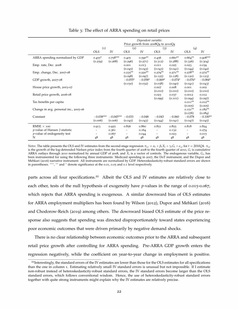
Table 3: The effect of ARRA spending on retail prices

Dependent variable:Price growth from 2008Q4 to 2010Q4

(1) (2) (3) (4)OLS IV OLS IV OLS IV OLS IV

ARRA spending normalized by GDP 0.455* 0.758*** 0.405 0.590** 0.456 0.660** 0.664** 0.908***(0.259) (0.268) (0.296) (0.271) (0.312) (0.288) (0.326) (0.304)

Emp. rate, Dec. 2008 0.001 0.013 0.011 0.025 0.023 0.039

(0.045) (0.043) (0.043) (0.041) (0.044) (0.042)Emp. change, Dec. 2007-08 0.235** 0.220** 0.279** 0.271** 0.278** 0.272**

(0.098) (0.097) (0.125) (0.128) (0.120) (0.123)GDP growth, 2007-08 −0.055* −0.058* −0.069* −0.074* −0.076* −0.084*

(0.030) (0.032) (0.038) (0.040) (0.041) (0.043)House price growth, 2003-07 0.007 0.008 0.001 0.002

(0.010) (0.010) (0.010) (0.010)Retail price growth, 2006-08 0.023 0.037 0.0012 0.012

(0.099) (0.101) (0.094) (0.097)Tax benefits per capita 0.011** 0.012**

(0.005) (0.005)Change in avg. personal inc., 2005-06 0.151** 0.182**

(0.076) (0.084)Constant −0.038*** −0.045*** −0.033 −0.048 −0.043 −0.060 −0.078 −0.100**

(0.006) (0.006) (0.045) (0.043) (0.044) (0.041) (0.047) (0.045)

RMSE × 100 0.913 0.925 0.856 0.860 0.851 0.855 0.818 0.824

p-value of Hansen J-statistic - 0.361 - 0.164 - 0.132 - 0.274

p-value of endogeneity test - 0.067 - 0.044 - 0.023 - 0.015

N 48 48 48 48 48 48 48 48

Notes: The table presents the OLS and IV estimates from the second-stage regression πi,t = αt + βtXi + γtGi + εi,t for t = 2010Q4. πi,tis the growth of the log-detrended Nielsen price index from the fourth quarter of 2008 to the fourth quarter of 2010, Gi is cumulativeARRA outlays through 2010 normalized by annual GDP of 2008, and Xi is a vector of controls. The endogenous variable, Gi , hasbeen instrumented for using the following three instruments: Medicaid spending in 2007, the DoT instrument, and the Dupor andMehkari (2016) narrative instrument. All instruments are normalized by GDP. Heteroskedasticity-robust standard errors are shownin parentheses. ∗∗∗, ∗∗ and ∗ denote significance at the 0.01, 0.05 and 0.1 level respectively.

parts across all four specifications.22 Albeit the OLS and IV estimates are relatively close to

each other, tests of the null hypothesis of exogeneity have p-values in the range of 0.015-0.067,

which rejects that ARRA spending is exogenous. A similar downward bias of OLS estimates

for ARRA employment multipliers has been found by Wilson (2012), Dupor and Mehkari (2016)

and Chodorow-Reich (2019) among others. The downward biased OLS estimate of the price re-

sponse also suggests that spending was directed disproportionately toward states experiencing

poor economic outcomes that were driven primarily by negative demand shocks.

There is no clear relationship between economic outcomes prior to the ARRA and subsequent

retail price growth after controlling for ARRA spending. Pre-ARRA GDP growth enters the

regression negatively, while the coefficient on year-to-year change in employment is positive.

22Interestingly, the standard errors of the IV estimates are lower than those for the OLS estimates for all specificationsthan the one in column 1. Estimating relatively small IV standard errors is unusual but not impossible. If I estimatenon-robust instead of heteroskedasticity-robust standard errors, the IV standard errors become larger than the OLSstandard errors, which follows conventional wisdom. Hence, the use of heteroskedasticity-robust standard errorstogether with quite strong instruments might explain why the IV estimates are relatively precise.

22

The coefficient on retail price growth before the ARRA is slightly negative but not estimated

with much precision.

I now turn to the dynamic response of prices over the entire sample period of 2006-2019,

which are shown in figure 3. OLS estimates are shown in the left panel, while the right panel

plots the IV estimates. Their 90 and 95% confidence bands are based on heteroskedasticity-robust

standard errors and indicated by dashed lines. As explained above, the estimates may be biased

after 2010 but I nonetheless present the estimates for the post-2010 period.

Figure 3: The dynamic effect of ARRA spending on retail prices

06 07 08 09 10 11 12 13 14 15 16 17 18 19

−1.00

−0.50

0.00

0.50

1.00

1.50

2.00

(a) OLS estimates

06 07 08 09 10 11 12 13 14 15 16 17 18 19

−1.00

−0.50

0.00

0.50

1.00

1.50

2.00

(b) IV estimates

Notes: The solid lines show the estimates of Γ = (γ1, γ2, . . . , γT) from the regression πi,t = αt + βtXi + γtGi + εi,t for t = 1, 2, . . . , T.πi,t is the growth of the log-detrended Nielsen price index relative to the fourth quarter of 2008, Gi is cumulative ARRA outlaysthrough 2010 normalized by GDP in 2008, and Xi is the vector of controls used in column 7-8 in table 3. The endogenous variable,Gi , has been instrumented for using Medicaid spending in 2007, the DoT instrument, and the Dupor and Mehkari (2016) narrativeinstrument. All instruments are normalized by GDP. The left panel shows the IV estimates, while the OLS estimates are shown in theright panel. Dashed lines indicate 95 and 90% confidence bands calculated using heteroskedasticity-robust standard errors. Verticallines indicate the enactment of the ARRA.

The estimates in figure 3 show that local ARRA spending caused a temporary increase in

local retail prices relative to other states. Estimates increase to around 1 after 1 year following the

spending shock and revert toward zero again about 4 to 5 years. Similar to the estimates reported

in table 3, the OLS estimates are lower than the IV estimates for the period after the ARRA. In

periods before the ARRA, the estimates fluctuate around zero, which indicates that there is no

correlation between pre-ARRA price movements and ARRA spending conditional on the control

variables.

Although the price index eventually reverts to trend, it takes 6 years so the response is rather

23

long-lived. However, this may be caused by the potential bias after 2010. I have tested the

overidentifying restriction quarter by quarter for all estimates of γt using the Hansen (1982)

J−statistic. While the statistics’ p-values are above any conventional value before 2011, they

occasionally drop below 0.1 thereafter. This indicates that the impulse response estimates after

2010 are indeed biased. Nonetheless, Cecchetti et al. (2002) have also estimated very persistent

effects of shocks on relative prices in U.S. cities, while Canova and Pappa (2007) find a hump-

shaped response of the price level to a state-financed government spending shock, which first

becomes insignificant at the 68% level after 6 years.

4.1 Robustness

I have explored the robustness of the estimates. The results are reported in Appendix C and

summarized below.

Pre-ARRA inflation dynamics I have explored whether or not states that received more stim-

ulus also had higher inflation rates before the enactment of the ARRA by using the state-level

CPIs by Nakamura and Steinsson (2014). Although this would not necessarily invalidate the

exclusion restriction, it could suggest that the results are spurious and reflect time-invariant in-

flation rate differentials not picked up by the controls. Reassuringly, the analysis in Appendix

C.1 shows that there is no systematic relationship between inflation dynamics during the period

of 1971-2008 and ARRA spending.

Alternative specifications Various robustness checks to the two-year price response estimates

in table 3 are reported in appendix table C.1.23 Rows 2 and 3 show that the estimates are robust

to normalizing ARRA spending by population or personal income instead of GDP. Rows 4 to

6 show the estimates when only using one instrument at a time. While the estimates from the

regressions using only the Medicaid or the narrative instrument are significant, the estimate from

the regression instrumenting with only the DoT instrument is insignificant.24 Row 7 includes the

squared and cubed pre-ARRA trend in retail prices, while row 8 includes bi-annual inflation

23Appendix figure C.2 show the dynamic response estimates from the robustness checks.24The first stage also suggests that the DoT instrument is not very powerful, which could bring noise into the IV

estimates. I have tried estimating the baseline regression without the DoT instrument but the resulting estimates andstandard errors are almost identical to the baseline.

24

rates in the years 2000 through 2006 based on the Nakamura and Steinsson (2014) CPIs in order

to control for pre-ARRA price growth in a more flexible manner. Neither affects the estimates

much, although controlling for bi-annual inflation in 2000-2006 lowers the estimate slightly. Row

9 replaces the price index with the alternative price index in which all UPCs and product modules

are weighted by annual national quantities and revenues (that is, weights are identical across

states, not time) to investigate if the baseline estimates reflect product-switching toward high

inflation products. The IV estimate is lowered by around a third but still significant. Row 10

presents estimates when using a fixed-base Laspeyres price index in which weights are fixed at

2006 values. This almost doubles the price response but prices still converge back to trend as

seen in panel (j) of appendix figure C.2. Finally, I include fixed effects for the 4 Census regions in

row 11. Although the point estimate for the last quarter of 2010 becomes lower and insignificant,

the dynamic response of prices is qualitatively similar to the baseline and significant in some

periods as seen in panel (k) of appendix figure C.2.

Outliers The added variable plot in appendix figure C.3 for price growth from the fourth quar-

ter of 2008 to the fourth quarter of 2010 against ARRA spending shows no indications of outlier-

driven estimates.

5 Evidence from military spending shocks

Figure 4 shows the main results from the analysis of military spending. This figure plots the

estimates of βh from regression (3.2) over 7 years with OLS estimates shown in the left panel

and IV estimates shown in the right panel. Each h-horizon regression is estimated separately

on a balanced panel of 377 MSAs, and the dashed lines indicate 90 and 95% confidence bands

based on pointwise standard errors. The error term, εi,t+h, is clustered by MSA to account for

within-MSA serial correlation. I winsorize local changes in military spending at the 1% level by

year to account for outliers in the data.

The IV estimates show that the response of retail prices is hump-shaped, statistically signifi-

cant and peaks around 0.07 after 3 years before it reverts to zero. This is equivalent to an increase

of 0.07% in retail prices when military spending increases by 1% of GDP. To get a sense of magni-

25

Figure 4: Response of retail prices to military spending

1 2 3 4 5 6 7

0.00

0.05

0.10

(a) OLS estimates

1 2 3 4 5 6 7

0.00

0.05

0.10

(b) IV estimates

Notes: The figure shows the estimates of βh from regression (3.2) estimated on a balanced panel of 377 MSAs. Panel (a) plots theOLS estimates, while IV estimates are plotted in panel (b). As control variables, the regression includes the lagged annual inflationrate and the lagged annual change in local spending normalized by GDP as well as its instrument. Dashed lines indicate 90 and 95%pointwise confidence bands based on standard errors clustered by MSA.

tudes, it is helpful to compare the estimates to the variation in the data. After controlling for year

and MSA fixed effects, the standard deviation of the three-year cumulative change in military

spending relative to GDP is 0.035, while the standard deviation of price growth over the same

period is 1.2%. Thus, a typical change in DoD spending of 3.5% of GDP over three years causes

an increase in prices of 0.07 · 0.035 = 0.25% or about 20% of the typical growth in prices observed

in the data.

Turning to the OLS estimates, they fluctuate around zero with relatively tight error bands.

As mentioned in section 3, it is not clear a priori in which direction the OLS estimates should be

biased since this will depend on the type of shocks hitting the MSAs. The bias, in this case is,

negative as is also the case for the ARRA estimates.

5.1 Comparison to estimates from the American Recovery and Reinvestment Act

Although military spending changes explain a non-negligible share of the variation in price

changes, the estimates are an order of magnitude lower than the estimates from the ARRA anal-

ysis in section 4. One reason for this could be that the geographical unit is smaller. For the case

of income multipliers, Demyanyk et al. (2018) find that military spending has larger effects as the

26

size of the geographic unit increases. This might be because spending is more likely to leak into

other areas as the geographic unit becomes smaller, which results in a smaller change in local

demand. In fact, Auerbach et al. (2020a) estimate that one dollar of military spending in an MSA

increases GDP in other MSAs in the same state by 0.58 dollars. Hence, their estimate indicates

that there are substantial geographic leakages.

Another reason why the estimates are smaller than those from the ARRA analysis could

be that military spending has little direct effect on the retail sector. Only 0.2% of the dollar

amount in the DoD contract data goes to food and beverage stores. Instead, the bulk of military

spending is directed at manufacturing and professional, scientific, and technical services. Thus,

the estimates do not capture direct demand effects on the retail sector but instead indirect effects

such as Keynesian income multiplier effects or factor demand effects.

Lastly, I show in section 5.3 below that prices respond more to military spending changes

when the local economy is slack. Since ARRA spending was outlaid during a period were all

states experienced high unemployment rates, this could explain why the estimates from the

ARRA analysis are larger than those from the military spending analysis.

5.2 Robustness

This section summarizes the results from a number of robustness checks of the baseline estimates,

which were shown in figure 4.

Alternative normalization of spending Columns 2 and 3 of appendix table A.2 report esti-

mates from regressions with the military spending variable normalized by personal income and

population instead of GDP. Both of these specifications deliver statistically significant estimates.

However, the estimates from the specification with military spending normalized by population

are not as significant as the baseline estimates.

Alternative instrument National military spending in the instrument is constructed using the

leave-one-out sum of spending and normalized by local GDP in period t. As mentioned above,

this induces MSA-specific variation in the aggregate component of the instrument over time. I

analyze the sensitivity of the estimates to this by constructing the instrument using the actual

27

change in national military spending and normalizing by local GDP as of 2005. The resulting

estimates are very close to those from the baseline specification as seen in column 4 of appendix

table A.2.

Alternative price indices Next, I estimate the regression using the two alternative price indices

to address the worry that the results are not driven by actual price changes but rather differences

in consumption composition across MSAs. Column 2 of appendix table A.3 shows that the price

response is close to the baseline estimates for the index with weights set to national values, while

the estimates from the fixed-base index in column 3 are substantially more imprecise. However,

the median number of products in the fixed-base index relative to the baseline index is only 3.6%

so the number of products entering the fixed-base index is typically quite low. This makes the

index more disposed to measurement error, which increases standard errors. This is illustrated

by the statistically significant estimates shown in column 4, where the fixed-base index is used

again but each MSA is weighted by the average number of products entering the fixed-base index

relative to the baseline index.

Correlates with spending shares The specifications in columns 2 to 4 of appendix table A.4

are motivated by the correlates of the military spending shares shown in table 2. First, I report

estimates in column 2 from a regression in which the MSAs are divided into quartiles based

on population density as of 2000 and then quartiles × year fixed effects are included. Hence,

the estimates are identified by variation within 4 groups of MSAs that are similar in terms of

population density. This tends to increase the estimates but also make them more imprecise

(albeit still statistically significant). Column 3 controls for differential inflation rates associated

with industry composition by adding two-digit industry employment shares as of 2005 interacted

with year dummies to the regression. The resulting estimates are similar although they are

slightly less precise. Column 4 addresses the worry that the estimates are driven by cross-

sectional differences in local retailer competition. I divide the MSAs into quartiles based on the

average number of grocery stores per capita over the sample period and then control for quartiles

× year fixed effects. The resulting estimates are close to the baseline.

28

Outliers Appendix table A.5 reports results from various checks of outliers in the data. Column

2 shows the estimates from a regression in which I remove the 10 MSAs with the highest share of

military spending (these MSAs are listed in appendix table A.6). One might worry that the MSAs

receiving most of the military spending are driving the estimates but the resulting estimates are

close to the baseline. Column 3 reports the estimates when using non-winsorized changes in

military spending, while the estimates in column 4 are from a regression in which I exclude

winsorized observations. The estimates from the former are lower than those from the baseline

regression, while the estimates from the latter are slightly larger. The instrument becomes weaker

when using non-winsorized changes in military spending (F-statistics are in range of 7-16). This

alone will bias the IV estimates toward the near-zero OLS estimates.

Decomposing variation I have explored if some areas drive the estimates. In order to this, I

follow Chodorow-Reich et al. (2021) and decompose the IV estimate, βh, into a weighted average

of estimates, βh,s, obtained from only using observations from each state s. The state-specific

weights sum to 1, and each weight is given by the contribution of each state s to the total residual

variation of the change in local military spending as predicted by the first stage.25 Appendix

figure D.4 illustrates the sensitivity of the baseline estimates to iteratively excluding one of the 5

states that receive the highest weights in the decomposition. These estimates are roughly similar

to the baseline estimates even though the top weight state, Pennsylvania, receives a weight of

34% in the decomposition of the baseline estimates. Hence, no single state drives the estimates.

The role of controls Appendix figure A.5 illustrates how the baseline IV estimates are affected

by the control variables. The estimates from the regression without any controls are almost

identical to those from a regression in which lagged inflation is controlled for. Adding the lagged

change in military spending and its instrument, however, has a sizeable effect on the estimates

up until the 2-year horizon. This is likely because these controls pick up the influence of prior

movements in military spending.26

25I relegate the details of this decomposition to Appendix D.26The lags of military spending changes and the instrument also enter significantly into the first stage, which

indicates that it is important to control for these variables in order to get unbiased estimates.

29

5.3 Price responses at high and low unemployment rates

A common view is that the presence of economic slack – idle resources commonly measured by

high rates of unemployment – causes changes in government spending to have a larger impact

on output. Indeed, prior papers have found evidence of larger output multipliers in regions

with a greater degree of slack (Nakamura and Steinsson, 2014; Demyanyk et al., 2018; Auerbach

et al., 2020a).27 However, there is a dearth of evidence on how the price response is shaped by

the amount of slack in the local economy. This is despite the fact that this can discipline which

mechanisms drive the differential response of output.

To test whether the price response differs by the amount of slack in the local economy, I re-

estimate regression (3.2) at the 1-year horizon but allow for the effect of government spending to

depend on slack using the following regression:

πi,t+1 = αi + ηt + βlGi,t+1 − Gi,t

Yi,t+ γlXi,t + Ii,t

[(βh − βl)

Gi,t+1 − Gi,t

Yi,t+ (γh − γl) Xi,t

]+ ε i,t+1,

(5.1)

where Ii,t is a dummy variable taking the value of 1 if the MSA is in a state of slack.

βl is an estimate of how military spending affects retail prices when the local economy is

not slack, while βh − βl captures the differential effect from slack. Economic slack is defined

in terms of the local unemployment rate at the start of the change in government spending. If

the unemployment rate at period t is above its median value over the sample period, I define

the MSA as being in a state of slackness, Ii,t = 1. Because of the high degree of business cycle

synchronization across locations in the U.S., the MSAs tend to almost all be slack or not in the

same years except for around 2008 and 2014.28

Column 1 in table 4 shows the IV estimates of the 1-year ahead response of prices to military

spending from regression (5.1). I also report estimates of the 1-year GDP multiplier by presence

of slack to connect the slack-dependent price response to the literature on slack-dependent out-

27The estimates from the literature using aggregate time series to estimate slack-dependent multipliers are lessclear-cut about whether multipliers are larger or smaller during times of economic slack. See e.g. Ramey and Zubairy(2018) and Barnichon et al. (forthcoming).

28According to the definition of slack as an unemployment rate above 6.5 by Ramey and Zubairy (2018), 2008 and2014 were also turning points, where the national U.S. economy switched to being slack and not slack respectively.

30

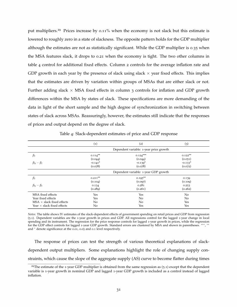
put multipliers.29 Prices increase by 0.11% when the economy is not slack but this estimate is

lowered to roughly zero in a state of slackness. The opposite pattern holds for the GDP multiplier

although the estimates are not as statistically significant. While the GDP multiplier is 0.35 when

the MSA features slack, it drops to 0.21 when the economy is tight. The two other columns in

table 4 control for additional fixed effects. Column 2 controls for the average inflation rate and

GDP growth in each year by the presence of slack using slack × year fixed effects. This implies

that the estimates are driven by variation within groups of MSAs that are either slack or not.

Further adding slack × MSA fixed effects in column 3 controls for inflation and GDP growth

differences within the MSA by states of slack. These specifications are more demanding of the

data in light of the short sample and the high degree of synchronization in switching between

states of slack across MSAs. Reassuringly, however, the estimates still indicate that the responses

of prices and output depend on the degree of slack.

Table 4: Slack-dependent estimates of price and GDP response

(1) (2) (3)

Dependent variable: 1-year price growth

βl 0.114** 0.124*** 0.122**(0.044) (0.044) (0.051)

βh − βl -0.141* -0.139* -0.133*(0.078) (0.078) (0.072)

Dependent variable: 1-year GDP growth

βl 0.211** 0.195** 0.139

(0.104) (0.097) (0.109)βh − βl 0.134 0.281 0.253

(0.289) (0.261) (0.262)

MSA fixed effects Yes Yes NoYear fixed effects Yes No NoMSA × slack fixed effects No No YesYear × slack fixed effects No Yes Yes

Notes: The table shows IV estimates of the slack-dependent effects of government spending on retail prices and GDP from regression(5.1). Dependent variables are the 1-year growth in prices and GDP. All regressions control for the lagged 1-year change in localspending and its instrument. The regression for the price response controls for lagged 1-year growth in prices, while the regressionfor the GDP effect controls for lagged 1-year GDP growth. Standard errors are clustered by MSA and shown in parentheses. ∗∗∗, ∗∗

and ∗ denote significance at the 0.01, 0.05 and 0.1 level respectively.

The response of prices can test the strength of various theoretical explanations of slack-

dependent output multipliers. Some explanations highlight the role of changing supply con-

straints, which cause the slope of the aggregate supply (AS) curve to become flatter during times

29The estimate of the 1-year GDP multiplier is obtained from the same regression as (5.1) except that the dependentvariable is 1-year growth in nominal GDP and lagged 1-year GDP growth is included as a control instead of laggedinflation.

31

of slack (Michaillat, 2014; Murphy, 2017). Other explanations rely on the aggregate demand (AD)

curve becoming more responsive to spending shocks (Eggertsson and Krugman, 2012; Rendahl,

2016). While both of these mechanisms result in a larger output multiplier, the price response

will differ. Whereas a flatter AS curve induces a smaller change in prices, a more responsive

AD curve will amplify the price response. The estimates in table 4 are thus consistent with the

changing slope of the AS curve dominating the effect from asymmetric shifts in the AD curve.30

Another common explanation of slack-dependent output multipliers is that central bankers

are less likely to lean against an increase in government spending when there is economic slack

and inflationary pressures are low. Because the stance of monetary policy is the same for regions

across the entire U.S., this can be ruled out as a driver since the effect on prices and output would

be captured by the time fixed effects in the regression. Of course, this does not imply that such a

mechanism does not actually exist but simply that this cross-regional framework cannot test its

presence.

6 Marginal costs or markups

The results in the previous two sections provided evidence of a positive response of local retail

prices to changes in government spending. The response can either be driven by changing

markups or a pass-through of marginal costs. This section shows that the response is likely to be

driven primarily by changing markups by controlling for changes in nominal marginal costs. I

focus on the analysis of military spending changes because of the panel data framework and the

larger number of observations, which give me more statistical power.

Unfortunately, the Nielsen data set does not include any information on costs so I rely on

other sources of data. For the entire grocery sector, however, wholesale costs make up around

three quarters of total costs (Stroebel and Vavra, 2019; Renkin et al., forthcoming). The sec-

ond largest cost component is labor costs, which constitute 12-13% of costs. Hence, I focus on

wholesale and labor costs.31

30The analysis by Demyanyk et al. (2018) indicates that both demand-side and supply-side mechanisms contributeto increasing the size of output multiplier in MSAs with slack economies.

31The remaining costs are mostly building and equipment expenses, which are likely fixed at shorter horizons.

32

6.1 Wholesale costs

Goods in the retail sector are rarely produced locally so wholesale costs should be insensitive to

local shocks (Stroebel and Vavra, 2019). Existing evidence from the U.S. retail sector also sug-

gests that wholesale costs vary little geographically. Using Nielsen PromoData which consists

of wholesale costs from one grocery wholesaler in each of 32 geographical areas, Stroebel and

Vavra (2019) show that wholesale costs only vary little geographically. For 26 of the 32 markets,

average wholesale costs are within 1% of the national average, while the most expensive area is

2.9% above the national average and the least expensive area is 2.3% below the national average.

Additionally, the wholesale price of 78% of the goods is exactly equal to the modal price. A sim-

ilar conclusion is reached by DellaVigna and Gentzkow (2019) who find no relationship between

local consumer income and wholesale costs when analyzing store-level data from a large U.S.

retail chain.

These findings suggest that regional variation in wholesale prices should not be able to ac-

count for regional variation in retail prices. However, if chains are segmented geographically and

they face similar wholesale costs – for example, due to using the same suppliers and selling the

same private-label products – or face common storage and transport costs, my estimates could

reflect pass-through from higher wholesale costs at the chain level. I investigate this by con-

structing MSA-level price indices for each of the 30 retail chains in the data using the procedure

described in section 2.1 and estimating equation (3.2) at the MSA × chain level:

πi,c,t+h = αi,c,h + ηc,t+h + βh∑h

k=1 (Gi,t+k − Gi,t)

Yi,t+ γhXi,c,t + ε i,c,t+h, (6.1)

where πi,c,t+h is the h-year inflation rate from period t to t+ h of chain c operating in MSA i. As in

equation (3.2), Gi,t is military spending in the MSA, where chain c operates, and the cumulative

change in local military spending is normalized by local initial GDP.

The regression includes MSA × chain fixed effects, αi,c,h, to control for the average inflation

rate of each chain within each MSA as well as year × chain fixed effects, ηc,t+h, which control for

the average inflation rate by year within each chain c. Thus, the regression controls for common

shocks to stores within a chain and identifies βh off price movements by stores belonging to the

33

same chain but located in different MSAs. Similar to regression (3.2), the set of control variables,

Xi,c,t, includes the lagged one-year change in military spending and its instrument as well the

lagged annual inflation rate of the MSA-chain pair, πi,c,t−1. Since military spending affects all

chains within an MSA equally, it is natural to also cluster the error term by MSA × year to

account for systematic over- or underprediction within an MSA by the model (Cameron and

Miller, 2015). Hence, I two-way cluster standard errors at the level of MSA × year to allow for

this intra-MSA correlation of chains’ error term within years, and at the level of MSA × chain to

allow for serial correlation of the error term within each chain-MSA pair.

The estimates of βh from regression (6.1) are presented in column 1 of table 5 and similar

to those from the MSA-level analysis presented in figure 4. This result is robust to controlling

for common chain-level shocks stores at a more geographically disaggregated level through the

inclusion of year × chain × Census division fixed effects in column 2. Column 3 shows the effect

of not controlling for chain-level shocks by replacing the year × chain fixed effects with year

effects. The resulting estimates and standard errors are almost twice as large as those in column

1. Overall, these estimates show that the baseline estimates are not driven only by a common

chain-level factor such as common changes in wholesale costs.

These results might seem surprising in light of the results by DellaVigna and Gentzkow (2019)

who find that chains in the Nielsen data tend to charge similar prices for the same products across

stores in different locations. These findings could lead one to think that local retail prices would

not react to a change in local military spending. Hence, it should be mentioned that a large

share of the variation in annual inflation across MSA-chain pairs can actually be attributed to a

common chain-level factor. Year × chain fixed effects alone can explain 82% of the variation in

annual inflation compared to the 39% explained by year fixed effects. Further adding year×MSA

fixed effects increases the share of variance explained to 89%. This underlines the importance

of controlling for common shocks to retailers belonging to the same chain but also that some

variation in inflation across different local markets is left unexplained by the common chain-level

factor.

34

Table 5: Controlling for common shocks to retail chains

(1) (2) (3)

1-year-horizon 0.033** 0.025* 0.028

(0.014) (0.014) (0.025)2-year-horizon 0.068*** 0.054** 0.110***

(0.022) (0.024) (0.041)3-year-horizon 0.055*** 0.049** 0.098**

(0.021) (0.020) (0.040)4-year-horizon 0.043*** 0.041** 0.080***

(0.016) (0.017) (0.030)5-year-horizon 0.028** 0.024** 0.042**

(0.011) (0.011) (0.019)6-year-horizon 0.021** 0.014 0.058***

(0.008) (0.009) (0.018)7-year-horizon 0.006 0.003 0.033*

(0.008) (0.008) (0.019)

Fixed effects Year × chain Year × chain × Censusdivision

Year

MSA × chain pairs 1484 1484 1484

Notes: The table presents the IV estimates of βh from equation (6.1). The regression only includes the 1,484 chain × MSA pairs thatare present in the entire period of 2006-2019, and local changes in military spending are winsorized using the same bounds as in theMSA-level regression. All regressions include chain × MSA fixed effects and control for one lag of annual price growth, the militaryspending change, and its instrument. Column 1 shows the estimates when including year × chain fixed effects, and column 2 showsthe estimates when controlling for year × chain × Census division fixed effects. Column 3 controls for year fixed effects. Standarderrors are shown in parenthesis and two-way clustered at the chain ×MSA and year ×MSA levels. *, **, and *** denotes significanceat the 10, 5, and 1 percent level respectively.

6.2 Labor costs and retailer entry/exit

Next, I control directly for factors that could affect labor costs. Although military spending

should not directly affect wages in the retail sector because very little spending is aimed at this

sector, it can raise average wages through effects on labor demand. Indeed, Auerbach et al.

(2020a) find evidence of military spending increasing wage earnings not only in industries ex-

posed to military spending either directly or through backward linkages but also in other indus-

tries, while Renkin et al. (forthcoming) show that increases in labor costs caused by minimum

wage hikes are fully passed through onto grocery store prices.

Column 2 in table 6 controls directly for the percentage change in the average wage in the

retail sector and shows that wage changes have no effect on the baseline estimates. This controls

for the intensive margin of labor costs but labor costs could also be affected by the hiring or

firing of staff. This is addressed in column 3 by controlling for the change in the employment

35

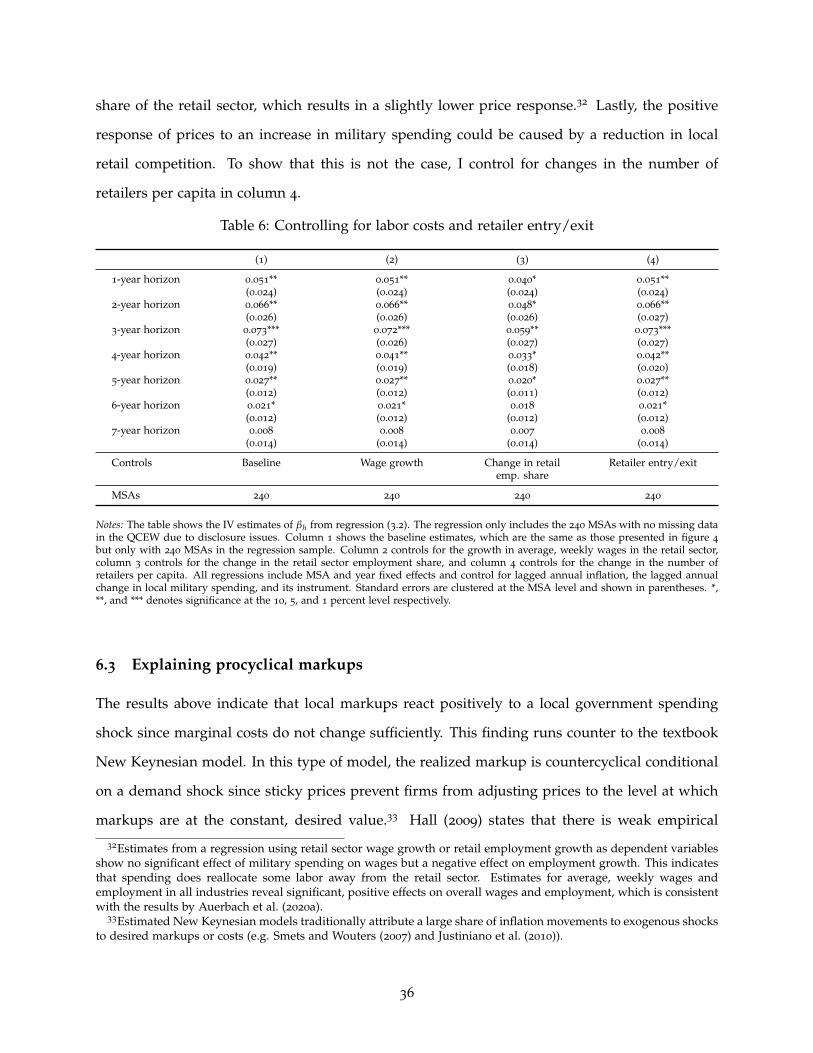
share of the retail sector, which results in a slightly lower price response.32 Lastly, the positive

response of prices to an increase in military spending could be caused by a reduction in local

retail competition. To show that this is not the case, I control for changes in the number of

retailers per capita in column 4.

Table 6: Controlling for labor costs and retailer entry/exit

(1) (2) (3) (4)

1-year horizon 0.051** 0.051** 0.040* 0.051**(0.024) (0.024) (0.024) (0.024)

2-year horizon 0.066** 0.066** 0.048* 0.066**(0.026) (0.026) (0.026) (0.027)

3-year horizon 0.073*** 0.072*** 0.059** 0.073***(0.027) (0.026) (0.027) (0.027)

4-year horizon 0.042** 0.041** 0.033* 0.042**(0.019) (0.019) (0.018) (0.020)

5-year horizon 0.027** 0.027** 0.020* 0.027**(0.012) (0.012) (0.011) (0.012)

6-year horizon 0.021* 0.021* 0.018 0.021*(0.012) (0.012) (0.012) (0.012)

7-year horizon 0.008 0.008 0.007 0.008

(0.014) (0.014) (0.014) (0.014)

Controls Baseline Wage growth Change in retailemp. share

Retailer entry/exit

MSAs 240 240 240 240

Notes: The table shows the IV estimates of βh from regression (3.2). The regression only includes the 240 MSAs with no missing datain the QCEW due to disclosure issues. Column 1 shows the baseline estimates, which are the same as those presented in figure 4

but only with 240 MSAs in the regression sample. Column 2 controls for the growth in average, weekly wages in the retail sector,column 3 controls for the change in the retail sector employment share, and column 4 controls for the change in the number ofretailers per capita. All regressions include MSA and year fixed effects and control for lagged annual inflation, the lagged annualchange in local military spending, and its instrument. Standard errors are clustered at the MSA level and shown in parentheses. *,**, and *** denotes significance at the 10, 5, and 1 percent level respectively.

6.3 Explaining procyclical markups

The results above indicate that local markups react positively to a local government spending

shock since marginal costs do not change sufficiently. This finding runs counter to the textbook

New Keynesian model. In this type of model, the realized markup is countercyclical conditional

on a demand shock since sticky prices prevent firms from adjusting prices to the level at which

markups are at the constant, desired value.33 Hall (2009) states that there is weak empirical

32Estimates from a regression using retail sector wage growth or retail employment growth as dependent variablesshow no significant effect of military spending on wages but a negative effect on employment growth. This indicatesthat spending does reallocate some labor away from the retail sector. Estimates for average, weekly wages andemployment in all industries reveal significant, positive effects on overall wages and employment, which is consistentwith the results by Auerbach et al. (2020a).

33Estimated New Keynesian models traditionally attribute a large share of inflation movements to exogenous shocksto desired markups or costs (e.g. Smets and Wouters (2007) and Justiniano et al. (2010)).

36

support for falling markups in response to higher government spending. This is also supported

by the recent cross-regional estimates by Auerbach et al. (2019). They find that the labor share –

which is typically linked to the inverse markup – falls slightly following an increase in military

spending. Similarly, Nekarda and Ramey (2020) conclude that markups are either procyclical or

acyclical irrespective of the type of shock hitting the economy after having revisited the markup

cyclicality literature with updated data and methods. Lastly, Anderson et al. (2018) study markup

fluctuations in the retail sector and find that they are mildly procyclical.

Some authors have focused on changes in consumers’ price sensitivity to explain why markups

might be procyclical. Stroebel and Vavra (2019) present evidence of homeowners becoming less

price sensitive as house prices increase because of positive wealth effects. This could cause re-

tailers’ to raise markups. This mechanism is specific to house price shocks but one could think

of a similar pricing mechanism for regional government spending shocks, where an increase in

government spending decreases households’ price sensitivity on average through positive effects

on employment and income. For example, Aguiar et al. (2013) find that unemployed workers

spend more time shopping relative to the employed, while Kaplan and Menzio (2015) find that

households with at least one unemployed household head pay 1-4% less for the same basket of

goods compared to fully employed households because they shop at a larger number of stores.

7 Concluding remarks

This paper studied how government spending affects retail prices by analyzing two spending

shocks: the state-level spending shock embedded in the ARRA of 2009 and MSA-level military

spending shocks. Both analyses revealed a positive effect of government spending on retail

prices. The ARRA estimates for the two-year response of retail price growth to an increase of

1% of GDP in government spending over the same period were in the range of 0.6-0.9%, while

the military spending estimates were more modest in size (around 0.06% over the same horizon).

Moreover, I find evidence of slack-dependent effects of changes in military spending. When the

local unemployment rate is high, the effect on prices is 0.14% but reduced to around zero when

the local unemployment rate is low.

I showed that the inflationary effects of the military spending shocks are unlikely to be driven

37

by changes in the marginal costs faced by retailers. This points towards a procyclical markup,

which stands in contrast to the predictions of a standard sticky-price model. As discussed above,

these findings are more in line with a strand of literature on the countercyclical nature of house-

holds’ shopping intensity, although none of these articles are directly concerned with the effects

of government spending. Whether government spending does affect households’ price sensi-

tivity is of course an empirical question. Hence, further research is needed to understand the

mechanism that can cause procyclical markups in reaction to demand shocks.

Finally, this paper only studied price movements in a sector that is unlikely to be affected di-

rectly by government spending shocks. Instead, I have argued that my estimates capture indirect

effects operating through variable markups. My results are silent on how price-setting and costs

are affected for firms supplying goods and services directly to the government. The military

contract data used in this paper, however, would be suitable for such an analysis.

38

References

Aguiar, M., Hurst, E., and Karabarbounis, L. (2013). Time Use During the Great Recession.

American Economic Review, 103(5):1664–1696.

Anderson, E., Rebelo, S., and Wong, A. (2018). Markups Across Space and Time. NBER Working

Paper No. 24434.

Auerbach, A., Gorodnichenko, Y., and Murphy, D. (2019). Macroeconomic Frameworks. NBER

Working Paper No. 26365.

Auerbach, A., Gorodnichenko, Y., and Murphy, D. (2020a). Local Fiscal Multipliers and Fiscal

Spillovers in the United States. IMF Economic Review, 68:195–229.

Auerbach, A. J., Gorodnichenko, Y., and Murphy, D. (2020b). Effects of Fiscal Policy on Credit

Markets. AEA Papers and Proceedings, 110:119–24.

Barnichon, R., Debortoli, D., and Matthes, C. (forthcoming). Understanding the Size of the

Government Spending Multiplier: It’s in the Sign. Review of Economic Studies.

Bartik, T. J. (1991). Who Benefits from State and Local Economic Development Policies? W.E. Upjohn

Institute.

Beraja, M., Hurst, E., and Ospina, J. (2019). The Aggregate Implications of Regional Business

Cycles. Econometrica, 87(6):1789–1833.

Bureau of Economic Analysis (2015). GDP by Metropolitan Area Methodology.

Cameron, A. C. and Miller, D. L. (2015). A Practitioner’s Guide to Cluster-Robust Inference.

Journal of Human Resources, 50(2):317–372.

Canova, F. and Pappa, E. (2007). Price Differentials in Monetary Unions: The Role of Fiscal

Shocks. The Economic Journal, 117(520):713–737.

Cecchetti, S. G., Mark, N. C., and Sonora, R. J. (2002). Price Index Convergence Among United

States Cities. International Economic Review, 43(4):1081–1099.

39

Chodorow-Reich, G. (2019). Geographic Cross-Sectional Fiscal Spending Multipliers: What Have

We Learned? American Economic Journal: Economic Policy, 11(2):1–34.

Chodorow-Reich, G., Feiveson, L., Liscow, Z., and Woolston, W. G. (2012). Does State Fiscal

Relief During Recessions Increase Employment? Evidence from the American Recovery and

Reinvestment Act. American Economic Journal: Economic Policy, 4(3):118–145.

Chodorow-Reich, G., Nenov, P. T., and Simsek, A. (2021). Stock Market Wealth and the Real

Economy: A Local Labor Market Approach. American Economic Review, 111(5):1613–57.

Coibion, O., Gorodnichenko, Y., and Hong, G. H. (2015). The Cyclicality of Sales, Regular and

Effective Prices: Business Cycle and Policy Implications. American Economic Review, 105(3):993–

1029.

Cox, L., Müller, G., Pastén, E., Schoenle, R., and Weber, M. (2020). Big G. NBER Working Paper

No. 27034.

D’Acunto, F., Malmendier, U., Ospina, J., and Weber, M. (2021). Exposure to Grocery Prices and

Inflation Expectations. Journal of Political Economy, 129(5):1615–1639.

D’Alessandro, A., Fella, G., and Melosi, L. (2019). Fiscal Stimulus with Learning-by-Doing.

International Economic Review, 60(3):1413–1432.

de Haan, J. and van der Grient, H. A. (2011). Eliminating chain drift in price indexes based on

scanner data. Journal of Econometrics, 161(1):36–46.

Del Negro, M. (1998). Aggregate Risk Sharing Across US States and Across European Countries.

Unpublished.

DellaVigna, S. and Gentzkow, M. (2019). Uniform Pricing in U.S. Retail Chains. The Quarterly

Journal of Economics, 134(4):2011–2084.

Demyanyk, Y., Loutskina, E., and Murphy, D. (2018). Fiscal Stimulus and Consumer Debt. The

Review of Economics and Statistics, 101(4):728–741.

Dubé, J.-P., Hitsch, G. J., and Rossi, P. E. (2018). Income and Wealth Effects on Private-Label

Demand: Evidence from the Great Recession. Marketing Science, 37(1):22–53.

40

Dupor, B., Karabarbounis, M., Kudlyak, M., and Mehkari, M. S. (2018). Regional Consumption

Responses and the Aggregate Fiscal Multiplier. Federal Reserve Bank of St. Louis, Working Paper

2018-004A.

Dupor, B. and McCrory, P. B. (2017). A Cup Runneth Over: Fiscal Policy Spillovers from the 2009

Recovery Act. The Economic Journal, 128(611):1476–1508.

Dupor, B. and Mehkari, M. S. (2016). The 2009 Recovery Act: Stimulus at the extensive and

intensive labor margins. European Economic Review, 85:208–228.

Eggertsson, G. B. and Krugman, P. (2012). Debt, Deleveraging, and the Liquidity Trap: A Fisher-

Minsky-Koo Approach. The Quarterly Journal of Economics, 127(3):1469–1513.

Forni, M. and Gambetti, L. (2016). Government spending shocks in open economy VARs. Journal

of International Economics, 99:68–84.

Gagnon, E. and López-Salido, D. (2020). Small Price Responses to Large Demand Shocks. Journal

of the European Economic Association, 18(2):792–828.

Goldsmith-Pinkham, P., Sorkin, I., and Swift, H. (2020). Bartik Instruments: What, When, Why,

and How. American Economic Review, 110(8):2586–2624.

Guren, A., McKay, A., Nakamura, E., and Steinsson, J. (2020). Housing Wealth Effects: The Long

View. The Review of Economic Studies, 88(2):669–707.

Gyourko, J., Saiz, A., and Summers, A. (2008). A New Measure of the Local Regulatory Envi-

ronment for Housing Markets: The Wharton Residential Land Use Regulatory Index. Urban

Studies, 45(3):693–729.

Hall, R. E. (2009). By How Much Does GDP Rise If the Government Buys More Output? Brookings

Papers on Economic Activity, 40(2 (Fall)):183–249.

Hansen, L. P. (1982). Large Sample Properties of Generalized Method of Moments Estimators.

Econometrica, 50(4):1029–1054.

Hitsch, G., Hortaçsu, A., and Lin, X. (2019). Prices and Promotions in U.S. Retail Markets:

Evidence from Big Data. NBER Working Paper No. 26306.

41

Jørgensen, P. L. and Ravn, S. H. (2021). The Inflation Response to Government Spending Shocks:

A Fiscal Price Puzzle? Unpublished.

Justiniano, A., Primiceri, G. E., and Tambalotti, A. (2010). Investment shocks and business cycles.

Journal of Monetary Economics, 57(2):132–145.

Kaplan, G. and Menzio, G. (2015). The Morphology of Price Dispersion. International Economic

Review, 56(4):1165–1206.

Kim, S. and Roubini, N. (2008). Twin deficit or twin divergence? Fiscal policy, current account,

and real exchange rate in the U.S. Journal of International Economics, 74(2):362–383.

Mian, A., Rao, K., and Sufi, A. (2013). Household Balance Sheets, Consumption, and the Eco-

nomic Slump. The Quarterly Journal of Economics, 128(4):1687–1726.

Mian, A. and Sufi, A. (2014). What Explains the 2007-2009 Drop in Employment? Econometrica,

82(6):2197–2223.

Michaillat, P. (2014). A Theory of Countercyclical Government Multiplier. American Economic

Journal: Macroeconomics, 6(1):190–217.

Monacelli, T. and Perotti, R. (2010). Fiscal Policy, the Real Exchange Rate and Traded Goods. The

Economic Journal, 120(544):437–461.

Montiel Olea, J. L. and Pflueger, C. (2013). A Robust Test for Weak Instruments. Journal of Business

& Economic Statistics, 31(3):358–369.

Murphy, D. (2017). Excess capacity in a fixed-cost economy. European Economic Review, 91:245 –

260.

Nakamura, E. and Steinsson, J. (2014). Fiscal Stimulus in a Monetary Union: Evidence from US

Regions. American Economic Review, 104(3):753–792.

Nekarda, C. and Ramey, V. (2020). The Cyclical Behavior of the Price-Cost Markup. Journal of

Money, Credit and Banking, 52(S2):319–353.

Ramey, V. A. (2011). Identifying Government Spending Shocks: It’s all in the Timing. The Quar-

terly Journal of Economics, 126(1):1–50.

42

Ramey, V. A. and Shapiro, M. D. (1998). Costly capital reallocation and the effects of government

spending. Carnegie-Rochester Conference Series on Public Policy, 48:145–194.

Ramey, V. A. and Zubairy, S. (2018). Government Spending Multipliers in Good Times and in

Bad: Evidence from US Historical Data. Journal of Political Economy, 126(2):850–901.

Ravn, M. O., Schmitt-Grohé, S., and Uribe, M. (2012). Consumption, government spending, and

the real exchange rate. Journal of Monetary Economics, 59(3):215–234.

Rendahl, P. (2016). Fiscal Policy in an Unemployment Crisis. The Review of Economic Studies,

83(3):1189–1224.

Renkin, T., Montialoux, C., and Siegenthaler, M. (forthcoming). The Pass-through of Minimum

Wages into US Retail Prices: Evidence from Supermarket Scanner Data. The Review of Economics

and Statistics.

Romer, C. D. and Romer, D. H. (2010). The Macroeconomic Effects of Tax Changes: Estimates

Based on a New Measure of Fiscal Shocks. American Economic Review, 100(3):763–801.

Saiz, A. (2010). The Geographic Determinants of Housing Supply. Quarterly Journal of Economics,

125(3):1253–1296.

Smets, F. and Wouters, R. (2007). Shocks and Frictions in US Business Cycles: A Bayesian DSGE

Approach. American Economic Review, 97(3):586–606.

Stock, J. H. and Watson, M. W. (2018). Identification and Estimation of Dynamic Causal Effects

in Macroeconomics Using External Instruments. The Economic Journal, 128(610):917–948.

Stroebel, J. and Vavra, J. (2019). House Prices, Local Demand, and Retail Prices. Journal of Political

Economy, 127(3):1391–1436.

Wilson, D. J. (2012). Fiscal Spending Jobs Multipliers: Evidence from the 2009 American Recovery

and Reinvestment Act. American Economic Journal: Economic Policy, 4(3):251–282.

43

A Additional figures and tables

Figure A.1: Slope estimates for state-specific trends (ARRA analysis)A

LA

RA

ZC

AC

O CT

DE FL GA IA ID IL IN KS

KY

LA MA

MD

ME

MI

MN

MO

MS

MT

NC

ND

NE

NH NJ

NM NV

NY

OH

OK

OR

PA RI

SC SD TN TX UT

VA VT

WA WI

WV

WY

0.008

0.010

0.012

0.014

0.016

0.018

0.020

0.022

Slop

eon

tren

d(a

nnua

lized

)

Notes: This figure plots the state-specific estimates of γ̃i from the regression ln pi,t = α̃i + γ̃i · t + ε̃i,t. The estimates have beenannualized by multiplying with 4 such that the figure shows the state-specific average annual growth rate in the price index. Errorbars indicate 95% confidence bands calculated using heteroskedasticity-robust standard errors.

44

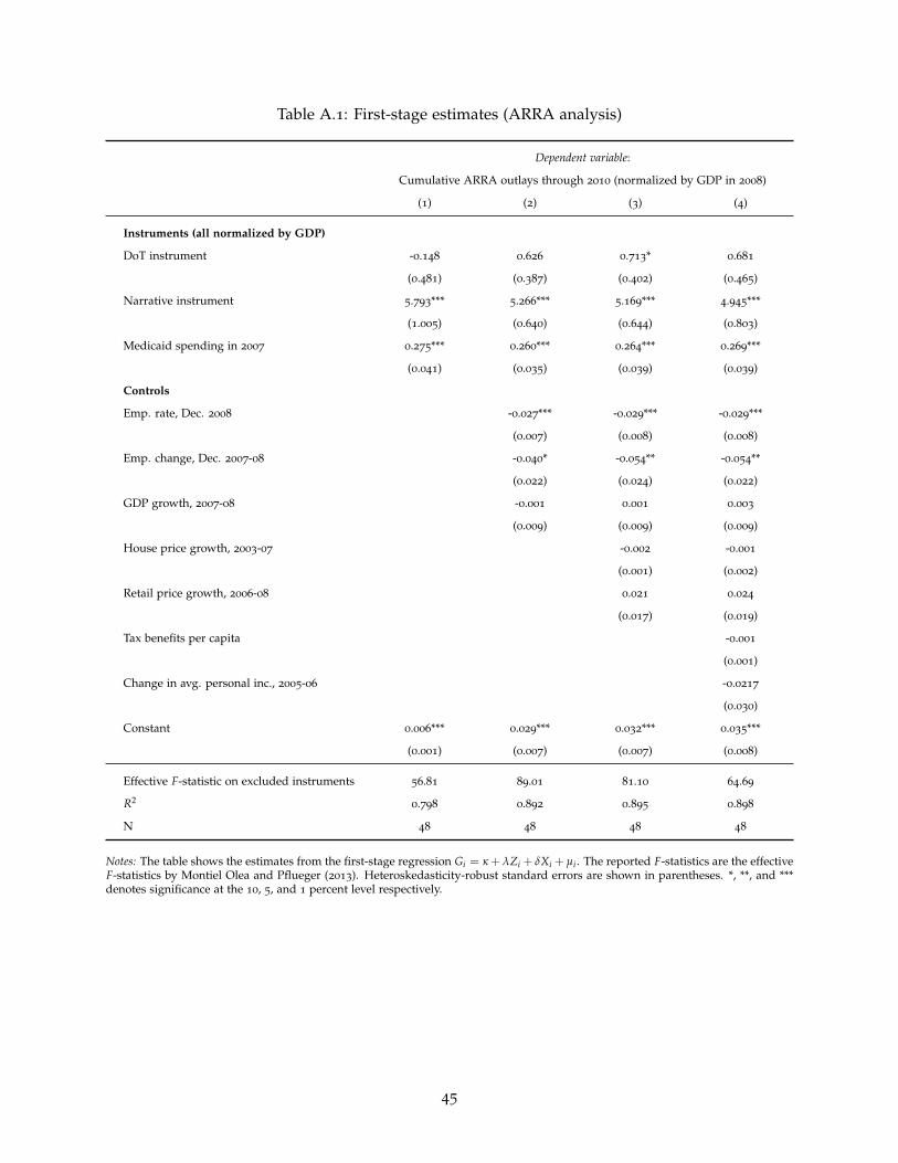
Table A.1: First-stage estimates (ARRA analysis)

Dependent variable:

Cumulative ARRA outlays through 2010 (normalized by GDP in 2008)

(1) (2) (3) (4)

Instruments (all normalized by GDP)

DoT instrument -0.148 0.626 0.713* 0.681

(0.481) (0.387) (0.402) (0.465)

Narrative instrument 5.793*** 5.266*** 5.169*** 4.945***

(1.005) (0.640) (0.644) (0.803)

Medicaid spending in 2007 0.275*** 0.260*** 0.264*** 0.269***

(0.041) (0.035) (0.039) (0.039)

Controls

Emp. rate, Dec. 2008 -0.027*** -0.029*** -0.029***

(0.007) (0.008) (0.008)

Emp. change, Dec. 2007-08 -0.040* -0.054** -0.054**

(0.022) (0.024) (0.022)

GDP growth, 2007-08 -0.001 0.001 0.003

(0.009) (0.009) (0.009)

House price growth, 2003-07 -0.002 -0.001

(0.001) (0.002)

Retail price growth, 2006-08 0.021 0.024

(0.017) (0.019)

Tax benefits per capita -0.001

(0.001)

Change in avg. personal inc., 2005-06 -0.0217

(0.030)

Constant 0.006*** 0.029*** 0.032*** 0.035***

(0.001) (0.007) (0.007) (0.008)

Effective F-statistic on excluded instruments 56.81 89.01 81.10 64.69

R20.798 0.892 0.895 0.898

N 48 48 48 48

Notes: The table shows the estimates from the first-stage regression Gi = κ + λZi + δXi + µi . The reported F-statistics are the effectiveF-statistics by Montiel Olea and Pflueger (2013). Heteroskedasticity-robust standard errors are shown in parentheses. *, **, and ***denotes significance at the 10, 5, and 1 percent level respectively.

45

Figure A.2: Distribution of predicted spending (ARRA analysis)

Notes: The heat map shows predicted ARRA spending normalized by GDP according to the first-stage regression without controls,Xi . Darker colors represent more spending.

Figure A.3: Distribution of military spending shares (military spending analysis)

Notes: The heat map shows the geographic distribution of the average annual military spending share over the period 2002-2005.Darker colors represent a higher share. A grey color indicates no spending.

46

Figure A.4: Kleibergen-Papp F-statistic (military spending analysis)

1 2 3 4 5 6 7 80

10

20

30

40

50

60

70

Estimation horizon

Kle

iber

gen-

Papp

F-st

atis

tic

Notes: The figure shows the Kleibergen-Papp F-statistic from the first-stage regression in the military spending analysis. Thehorizontal, dashed line indicates the Montiel Olea and Pflueger (2013) critical value for the F-statistic under a null hypothesis of theIV bias exceeding 10% of the OLS bias at the 5 percent significance level.

Table A.2: Robustness to alternative specifications (military spending analysis)

(1) (2) (3) (4)

1-year horizon 0.052** 0.040* 0.008** 0.057**(0.025) (0.022) (0.004) (0.025)

2-year horizon 0.062** 0.046** 0.007* 0.062**(0.026) (0.021) (0.004) (0.025)

3-year horizon 0.070*** 0.060** 0.013** 0.069***(0.027) (0.024) (0.006) (0.023)

4-year horizon 0.039* 0.031* 0.005 0.036*(0.021) (0.018) (0.004) (0.020)

5-year horizon 0.028** 0.023** 0.003 0.027**(0.014) (0.011) (0.003) (0.012)

6-year horizon 0.025* 0.022* 0.002 0.023*(0.015) (0.013) (0.003) (0.014)

7-year horizon 0.015 0.012 0.001 0.007

(0.017) (0.015) (0.003) (0.013)

Robustness Baseline Spendingnormalized by

income

Spendingnormalized by

population

Alternativeinstrument

MSAs 377 377 377 377

Notes: The table shows IV estimates from robustness checks of the estimates of βh from regression (3.2). Column 1 are the baselineestimates shown in figure 4. Column 2 normalizes the change in military spending by personal income, while column 3 normalizesthe change in military spending by population and scales estimates by 1000. Column 4 instruments for military spending changeswith the pre-sample share of national spending interacted with the actual change in national military spending normalized by MSA-level GDP as of 2005. All specifications include the control variables from the baseline specification and MSA and year fixed effects.Error terms are clustered by MSA. Standard errors are shown in parentheses. *, **, and *** denotes significance at the 10, 5, and 1

percent level respectively.

47

Table A.3: Robustness to alternative price indices (military spending analysis)

(1) (2) (3) (4)

1-year horizon 0.052** 0.059** 0.074 0.12*(0.025) (0.028) (0.060) (0.060)

2-year horizon 0.062** 0.071*** 0.043 0.10*(0.026) (0.026) (0.056) (0.060)

3-year horizon 0.070*** 0.070*** 0.084 0.13**(0.027) (0.022) (0.060) (0.054)

4-year horizon 0.039* 0.043** 0.025 0.060

(0.021) (0.021) (0.053) (0.053)5-year horizon 0.028** 0.033*** 0.007 0.034

(0.014) (0.011) (0.034) (0.036)6-year horizon 0.025* 0.034*** 0.006 0.030

(0.015) (0.010) (0.028) (0.030)7-year horizon 0.015 0.022 -0.014 -0.007

(0.017) (0.013) (0.033) (0.042)

Robustness Baseline Equal weights index Fixed-base index Fixed-base index(weighted estimates)

MSAs 377 377 377 377

Notes: The table shows IV estimates from robustness checks of the estimates of βh from regression (3.2). Column 1 are the baselineestimates shown in figure 4. Column 2 uses a Laspeyres price index with weights set to the their national quantities and revenues,while column 3 uses a fixed-base Laspeyres index with weights fixed at quantities and revenues as of 2007. Column 4 uses a fixed-base Laspeyres index and weights each MSA by the average number of products in the fixed-base index relative to the baselinechained index. All specifications include the control variables from the baseline specification and MSA and year fixed effects. Errorterms are clustered by MSA. Standard errors are shown in parentheses. *, **, and *** denotes significance at the 10, 5, and 1 percentlevel respectively.

Table A.4: Robustness to possible confounders (military spending analysis)

(1) (2) (3) (4)

1-year horizon 0.052** 0.046 0.037 0.056**(0.025) (0.030) (0.031) (0.023)

2-year horizon 0.062** 0.083** 0.071** 0.072**(0.026) (0.036) (0.034) (0.029)

3-year horizon 0.070*** 0.072* 0.063* 0.075***(0.027) (0.041) (0.036) (0.028)

4-year horizon 0.039* 0.044 0.033 0.045**(0.021) (0.028) (0.028) (0.020)

5-year horizon 0.028** 0.040** 0.026 0.033**(0.014) (0.021) (0.020) (0.014)

6-year horizon 0.025* 0.043** 0.029 0.030*(0.015) (0.022) (0.018) (0.016)

7-year horizon 0.015 0.019 0.028 0.018

(0.017) (0.025) (0.026) (0.016)

Robustness Baseline Pop. density × yearfixed effects

Industry shares ×year dummies

Avg. products perstore × year fixed

effects

MSAs 377 371 377 377

Notes: The table shows IV estimates from robustness checks of the estimates of βh from regression (3.2). Column 1 are the baselineestimates shown in figure 4. Column 2 controls for population density quartiles × year fixed effects. Column 3 controls for two-digitNAICS employment shares as of 2005 interacted with year dummies. Column 4 controls for average products per store quartiles× year fixed effects. All specifications include the control variables from the baseline specification and MSA and year fixed effects.Error terms are clustered by MSA. Standard errors are shown in parentheses. *, **, and *** denotes significance at the 10, 5, and 1

percent level respectively.

48

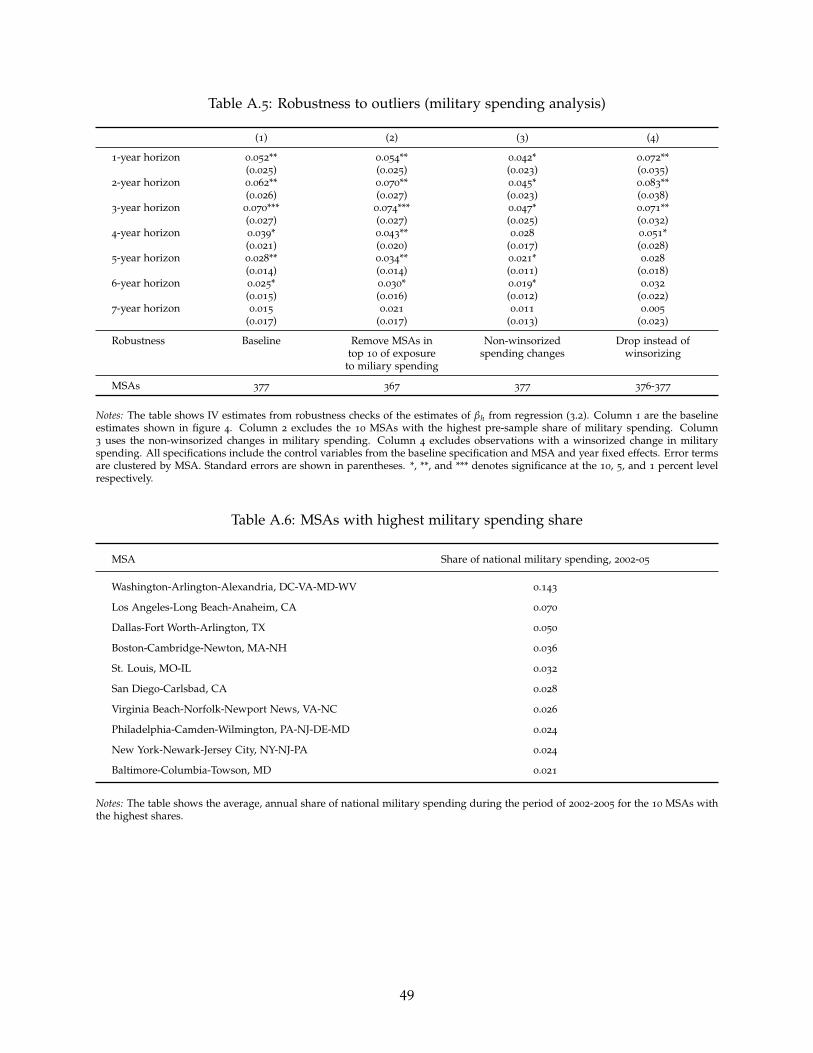
Table A.5: Robustness to outliers (military spending analysis)

(1) (2) (3) (4)

1-year horizon 0.052** 0.054** 0.042* 0.072**(0.025) (0.025) (0.023) (0.035)

2-year horizon 0.062** 0.070** 0.045* 0.083**(0.026) (0.027) (0.023) (0.038)

3-year horizon 0.070*** 0.074*** 0.047* 0.071**(0.027) (0.027) (0.025) (0.032)

4-year horizon 0.039* 0.043** 0.028 0.051*(0.021) (0.020) (0.017) (0.028)

5-year horizon 0.028** 0.034** 0.021* 0.028

(0.014) (0.014) (0.011) (0.018)6-year horizon 0.025* 0.030* 0.019* 0.032

(0.015) (0.016) (0.012) (0.022)7-year horizon 0.015 0.021 0.011 0.005

(0.017) (0.017) (0.013) (0.023)

Robustness Baseline Remove MSAs intop 10 of exposure

to miliary spending

Non-winsorizedspending changes

Drop instead ofwinsorizing

MSAs 377 367 377 376-377

Notes: The table shows IV estimates from robustness checks of the estimates of βh from regression (3.2). Column 1 are the baselineestimates shown in figure 4. Column 2 excludes the 10 MSAs with the highest pre-sample share of military spending. Column3 uses the non-winsorized changes in military spending. Column 4 excludes observations with a winsorized change in militaryspending. All specifications include the control variables from the baseline specification and MSA and year fixed effects. Error termsare clustered by MSA. Standard errors are shown in parentheses. *, **, and *** denotes significance at the 10, 5, and 1 percent levelrespectively.

Table A.6: MSAs with highest military spending share

MSA Share of national military spending, 2002-05

Washington-Arlington-Alexandria, DC-VA-MD-WV 0.143

Los Angeles-Long Beach-Anaheim, CA 0.070

Dallas-Fort Worth-Arlington, TX 0.050

Boston-Cambridge-Newton, MA-NH 0.036

St. Louis, MO-IL 0.032

San Diego-Carlsbad, CA 0.028

Virginia Beach-Norfolk-Newport News, VA-NC 0.026

Philadelphia-Camden-Wilmington, PA-NJ-DE-MD 0.024

New York-Newark-Jersey City, NY-NJ-PA 0.024

Baltimore-Columbia-Towson, MD 0.021

Notes: The table shows the average, annual share of national military spending during the period of 2002-2005 for the 10 MSAs withthe highest shares.

49

Figure A.5: Robustness to controls (military spending analysis)

1 2 3 4 5 6 7

0.00

0.05

0.10

No controlsWith lagged price growthWith lagged spending change and instrumentWith all controls

Notes: The figure shows the IV estimates of βh from regression (3.2) using various control variables.

50

B Description of the ARRA instrumnents

This appendix provides information on the instruments used in the analysis of the ARRA.

The Medicaid instrument The Medicaid spending instrument by Chodorow-Reich et al. (2012)

exploits that the ARRA set up an $87 billion State Fiscal Relief Fund to aid states in paying

Medicaid expenses. This was one of the first ARRA components to affect the economy with aid

payments already flowing to states by March 2009. Before the ARRA was passed, the federal

government reimbursed 50 to 83% of states’ Medicaid expenses according to state-specific re-

imbursement rates (the Federal Medical Assistance Percentages, or FMAP). The reimbursement

scheme is set up such that poorer states – which tend to have larger Medicaid expenses – have

a higher FMAP. Each state’s rate was recalculated every fiscal year based on a three-year trail-

ing average of the state’s per capita personal income relative to the national average. With the

passage of the ARRA, states’ FMAP could not decrease from their 2008 level, and all states’

FMAP were raised by 6.2 percentage points. Thus, states with larger Medicaid expenses prior

to the ARRA received a larger transfer from the State Fiscal Relief Fund, and Medicaid expenses

in 2007 can be used as an instrument for this transfer. Although state governments could use

the transfer for any purpose, Chodorow-Reich et al. (2012) argue that states did not retain the

transfer on their budgets.34

The Department of Transportation instrument Around three quarters of the DoT’s $40 bil-

lion ARRA funding was allocated to the Federal Highway Administration (FHWA). 50% of these

funds were divided among states based on a pre-existing allocation formula, which is a weighted

average of three factors measured with a three-year lag: miles of federal-aid highway, vehicle-

miles traveled on federal-aid highways, and payments into the federal highway trust fund. The

remaining 50% of the funds were allocated in proportion to the 2008 FHWA obligation limita-

tions on funding for each state’s Federal-Aid Highway Programs. Hence, an instrument can be

constructed by taking the fitted values from a regression of total DoT ARRA funding on the

34Additionally, the positive employment effects estimated by Chodorow-Reich et al. (2012) are concentrated insectors relying on state funds – the state and local government, health and education sectors – which suggest that thetransfers were used to avoid state program cuts.

51

miles of federal-aid highway in 2006, estimated vehicle-miles traveled on federal-aid highways

in 2006, estimated payments into the federal highway trust fund in 2006, and FHWA obligation

limitations in 2008.35

Dupor and Mehkari instrument Dupor and Mehkari (2016) take the logic of the two other

instruments to the extreme by classifying components of the ARRA that were exogenous to local

economic conditions using a narrative approach similar to that of Romer and Romer (2010) and

Ramey (2011). They found these components by reading through the provisions of the ARRA as

well as the federal codes and regulations used to allocate stimulus. If the criteria for allocation of

funds were plausibly exogenous to the local business cycle, they deemed the funds as exogenous.

For example, one exogenous component is around $6 billion of funds that were authorized to

urbanized areas (UZAs) to improve public transit capital under the Capital Transit Assistance

program. UZAs with a population between 50,000 and 199,999 persons received funds based on

their population and population density, while UZAs with a higher population received funds

according to a number of factors such as bus passenger miles and bus revenue vehicle miles.

After adding up all exogenous components, the instrument identifies $21.5 billion by the end of

2010.

35Standard errors in the first and second-stage regressions should in principle be adjusted for the use of fitted valuesas an instrument. However, I do not since the four factors explain almost all of the variation in DoT spending.

52

C ARRA analysis: Robustness

This appendix presents robustness checks to the estimates from the ARRA analysis.

C.1 Pre-ARRA inflation dynamics

One worry is that states receiving more ARRA spending might have had higher inflation rates

before the enactment of the law that are not captured by the controls and the state-specific log-

linear trend. If this is the case, the estimate for the response of retail prices to spending could

be spurious. Unfortunately, the Nielsen price index can only be constructed from 2006, which is

insufficient to uncover any such long-run differences in price dynamics prior to the ARRA.

Instead, I rely on annual CPI series by Nakamura and Steinsson (2014). Their CPIs cover the

period of 1969-2006 and are imputed from several sources. From 1969 until 1995 they use CPIs

constructed by Del Negro (1998). After 1995 they construct state-level indices by multiplying the

U.S. aggregate CPI with population-weighted cost of living indices from the American Chamber

of Commerce Realtors Association.

I estimate 38 versions of regression (3.1) in which I replace the dependent variable with the

two-year inflation rate, πNMi,t , from the Nakamura and Steinsson (2014) data set from 1971 until

2008:

πNMi,t = αt + γtGi + βtXi + εi,t for t = 1971, 1972, . . . , 2008, (C.1)

where the full set of controls and instruments from the baseline regression are included.

The empirical cumulative distribution function for γt using the 38 placebo IV estimates are

shown in figure C.1. The estimate for the response of retail prices in the fourth quarter of 2010 is

indicated by the vertical, dashed line.

If the estimates presented in section 3 reflect a spurious correlation between the average

inflation rate and ARRA spending, the placebo estimates would be positive on average. This is

not the case: the median placebo estimate is close to zero. These findings are also in line with the

placebo analysis by Chodorow-Reich et al. (2012) for ARRA employment multipliers. Only five of

the placebo estimates are above the retail price response estimate of 0.9. Keep in mind, however,

53

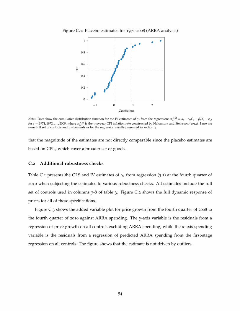
Figure C.1: Placebo estimates for 1971-2008 (ARRA analysis)

−1 0 1 2

0

0.2

0.4

0.6

0.8

1

Coefficient

CD

F

Notes: Dots show the cumulative distribution function for the IV estimates of γt from the regressions πNMi,t = αt + γtGi + βtXi + εi,t

for t = 1971, 1972, . . . , 2008, where πNMi,t is the two-year CPI inflation rate constructed by Nakamura and Steinsson (2014). I use the

same full set of controls and instruments as for the regression results presented in section 3.

that the magnitude of the estimates are not directly comparable since the placebo estimates are

based on CPIs, which cover a broader set of goods.

C.2 Additional robustness checks

Table C.1 presents the OLS and IV estimates of γt from regression (3.1) at the fourth quarter of

2010 when subjecting the estimates to various robustness checks. All estimates include the full

set of controls used in columns 7-8 of table 3. Figure C.2 shows the full dynamic response of

prices for all of these specifications.

Figure C.3 shows the added variable plot for price growth from the fourth quarter of 2008 to

the fourth quarter of 2010 against ARRA spending. The y-axis variable is the residuals from a

regression of price growth on all controls excluding ARRA spending, while the x-axis spending

variable is the residuals from a regression of predicted ARRA spending from the first-stage

regression on all controls. The figure shows that the estimate is not driven by outliers.

54

Table C.1: Robustness checks (ARRA analysis)

Specification OLS IV

(1) Baseline 0.664** 0.908***(0.326) (0.304)

(2) Spending normalized by population 0.008 0.019**(0.008) (0.008)

(3) Spending normalized by personal income 0.387 0.806**(0.357) (0.367)

(4) Only Medicaid instrument 0.664* 1.264***(0.326) (0.406)

(5) Only DoT instrument 0.664** 0.883

(0.326) (0.555)(6) Only narrative instrument 0.664** 0.679**

(0.326) (0.306)(7) Control for squared and cubed pre-trend 0.646* 0.894***

(0.352) (0.342)(8) Control for bi-annual CPI inflation 2000-06 0.784** 0.795***

(0.260) (0.270)(9) Use equal weights price index 0.535*** 0.580***

(0.197) (0.213)(10) Use fixed-base price index 1.245*** 1.508***

(0.443) (0.481)(11) Include region dummies 0.265 0.370

(0.271) (0.313)

Notes: The table presents the OLS and IV estimates from the regression πi,t = αt + βtXi + γtGi + εi,t for t = 2010Q4. πi,t isthe growth of the retail price index from the last quarter of 2008 to the last quarter of 2010, Gi are cumulative ARRA outlaysthrough 2010 normalized by GDP in 2008, and Xi is a vector of controls. The endogenous variable, Gi , has been instrumented forusing the three instruments described in section 4: Medicaid spending in 2007, the DoT instrument, and the Dupor and Mehkari(2016) narrative measure. In the regressions using the growth of the equal weights and fixed-base price indices as a dependentvariable (row 9-10), the pre-ARRA trend in retail prices is measured using the equal weight and fixed-base price indices respectively.Heteroskedasticity-robust standard errors are shown in parentheses. ∗∗∗, ∗∗ and ∗ denote significance at the 0.01, 0.05 and 0.1 levelrespectively.

55

Figure C.2: Dynamic IV estimates from robustness checks (ARRA analysis)

0607080910111213141516171819

-2.25

-1.50

-0.75

0.00

0.75

1.50

2.25

3.00

(a) Baseline

0607080910111213141516171819

-0.025

0.000

0.025

0.050

(b) Normalize ARRA by pop.

0607080910111213141516171819

-2.25

-1.50

-0.75

0.00

0.75

1.50

2.25

3.00

(c) Normalize ARRA by inc.

0607080910111213141516171819

-2.25

-1.50

-0.75

0.00

0.75

1.50

2.25

3.00

(d) Medicaid inst. only

0607080910111213141516171819

-2.25

-1.50

-0.75

0.00

0.75

1.50

2.25

3.00

(e) DoT inst. only

0607080910111213141516171819

-2.25

-1.50

-0.75

0.00

0.75

1.50

2.25

3.00

(f) Narrative inst. only

0607080910111213141516171819

-2.25

-1.50

-0.75

0.00

0.75

1.50

2.25

3.00

(g) Include squared and cubedpre-trend

0607080910111213141516171819

-2.25

-1.50

-0.75

0.00

0.75

1.50

2.25

3.00

(h) Control for bi-annual CPIinflation 2000-06

0607080910111213141516171819

-2.25

-1.50

-0.75

0.00

0.75

1.50

2.25

3.00

(i) Use equal weights price in-dex

0607080910111213141516171819

-2.25

-1.50

-0.75

0.00

0.75

1.50

2.25

3.00

(j) Use fixed-base price index

0607080910111213141516171819

-2.25

-1.50

-0.75

0.00

0.75

1.50

2.25

3.00

(k) Include region dummies

Notes: The figures show IV estimates over the entire sample period for the robustness checks also provided in table C.1. All regres-sions include the full set of controls included in column 4 of table 3. 90% and 95% confidence bands based on heteroskedasticity-robust standard errors are indicated by dashed lines. The vertical dashed lines indicate the enactment of the ARRA.

56

Figure C.3: Price growth against government spending (ARRA analysis)

−0.01 −0.01 0.00 0.01 0.01 0.02

−0.02

0.00

0.02

0.04

AL

AZAR

CACO

CTDE

FL

GA ID

IL IN

IA

KS

KY

LA

ME

MD

MA

MI

MN

MSMO

MT

NE NV

NH

NJ

NMNY

NCND

OH

OK

OR

PA

RI

SC

SD

TN

TX

UTVT

VA

WA

WVWIWY

Predicted ARRA spending normalized by GDP

Pric

egr

owth

Notes: The figure shows the added variable plot for price growth against ARRA spending from regression (3.1). The y-axis variableis the residuals from a regression of price growth from the fourth quarter of 2008 to the fourth quarter of 2010 on all controlsexcluding ARRA spending, while the x-axis spending variable is the residuals from a regression of predicted ARRA spending fromthe first-stage regression on all controls.

57

D Military spending analysis: Decomposing variation

This appendix provides details on the decomposition of the IV estimates presented in section 5.2.

This decomposition builds on the decomposition of the OLS estimator by Chodorow-Reich et al.

(2021) but applied to IV estimates.

The h horizon IV estimate from regression (3.2) can be decomposed as follows:

βh =(G̃′hG̃h

)−1 G̃′hΠ̃h = ∑s

wh,sβh,s, (D.1)

wh,s =(G̃′hG̃h

)−1 G̃′h,sG̃h,s (D.2)

βh,s =(G̃′hG̃h

)−1 G̃′h,sΠ̃h,s. (D.3)

G̃h is the vector of predicted h horizon changes in military spending according to the first

stage residualized by the predicted control variables from the first stage. Similarly, Π̃h is the

vector of h horizon price growth residualized by the predicted control variables from the first

stage. G̃h,s and Π̃h,s are subsets of these two vectors for MSAs belonging to state s. Although

this decomposition is done by dividing MSAs into states, the decomposition can be done for any

non-overlapping partition of the data set.

The weights sum to 1 and each weight, ws, is the contribution of state s to the total residual

variation in the military spending changes. It should be noted that βh,s is not equal to the IV

estimate from a regression with only state s. This is because the first stage estimates and the

coefficients on the controls will generally vary across states. That is, the decomposition imposes

these relationships from the full sample onto the individual βh,s estimates.

The decomposition is easy to perform in 3 steps:

1. Get the predicted values of the endogenous variable and the controls from the first-stage

regression.

2. Residualize the dependent variable and the predicted endogenous regressor with the pre-

dicted control variables to get G̃h and Π̃h.

3. Use G̃h and Π̃h to construct the set of state-specific weights and estimates, ws and βh,s.

58

I calculate the weights for h = 3 but the ranking of weights across states is similar for other

horizons. Figure D.4 shows the baseline IV estimates for the whole sample as well as 5 sets of

estimates for which I drop one of the top 5 weight states in each set.

Figure D.4: Sensitivity of estimates to important states

1 2 3 4 5 6 70.00

0.02

0.04

0.06

0.08

0.10BaselineWithout Pennsylvania (weight = 0.34)Without Connecticut (weight = 0.15)Without Alabama (weight = 0.09)Without Wisconsin (weight = 0.07)Without Florida (weight = 0.06)

Notes: The figure shows the IV estimates from regression (3.2) when dropping MSAs from one of the top 5 weight states accordingto the decomposition in equations (D.1) to (D.3).

59

W O R K I N G P A P E R — D A N M AR K S N A T IO N A L B A N K

8 S E P T E M B ER 20 21 — NO . 18 1

As a rule, Working Papers are not translated, but are available in the original language used by the contributor. Danmarks Nationalbank's Working Papers are published in PDF format at www.nationalbanken.dk. A free electronic subscription is also available on the website. The subscriber receives an e-mail notification whenever a new Working Paper is published. Text may be copied from this publication provided that the source is specifically stated. Changes to or misrepresentation of the content are not permitted. Please direct any enquiries directly to the contributors or to Danmarks Nationalbank, Communications, Kommunikation@nationalbanken.dk.