Embed Size (px)
Citation preview

Copyright © 2014 McGraw-Hill Education. All rights reserved. No reproduction or distribution without the prior written consent of McGraw-Hill Education.
Chapter 6
Government Interven1on

6-2
What will you learn in this chapter? • What effect a price ceiling or a price floor has on the equilibrium price and quan1ty.
• What effect a tax or a subsidy has on the equilibrium price and quan1ty.
• How elas1city and 1me period influence the impact of a market interven1on.

6-3
Why intervene? • Markets gravitate toward equilibrium. • When markets work well, prices adjust un1l the quan1ty of the good demanded is equal to the quan1ty supplied.
• There are three reasons why a government may step in and intervene in a market: – Correc1ng market failures. – Changing the distribu1on of benefits. – Encouraging or discouraging consump1on of certain goods.

6-4
Four real-‐world interven7ons • In this chapter, four real-‐world examples of government interven1on will be analyzed. – Mexican tor1lla prices and the government seNng a maximum price.
– U.S. milk prices and the government seNng a minimum price.
– U.S. faQy foods and the government taxing high fat and high calorie foods.
– Mexican tor1lla prices and the government subsidizing tor1lla producers.
• These examples require both posi1ve and norma1ve analysis. – What are the trade-‐offs? – Do the benefits outweigh the costs?

6-5
Price controls • Price controls can be divided into categories:
– Price ceiling: A maximum legal price at which a good can be sold.
• Typically placed on essen1al goods and services such as food, gasoline, and electricity.
– Price floor: A minimum legal price at which a good can be sold.
• Typically placed on agricultural goods that are risky to produce.
• The price controls provide incen1ves or disincen1ves to produce more or less than the equilibrium quan1ty.
6-6
Price ceilings
0
25
50
75
100
125
25 50 75 100 Quantity of tortillas (millions of lbs.)
S
D
Price (¢/lb.)
0
25
50
75
100
125
25 50 75 100
Price (¢ / lb.)
Quantity of tortillas (millions of lbs.) Shortage
S
D
Producers supply a lower quantity.
Consumers demand a higher quantity.
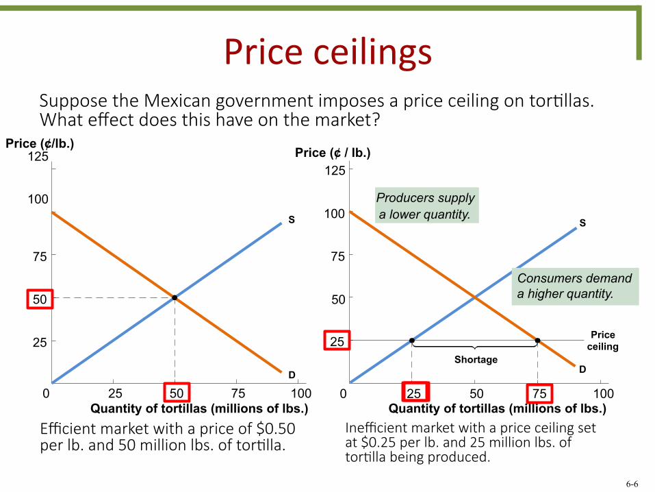
Suppose the Mexican government imposes a price ceiling on tor1llas. What effect does this have on the market?
Efficient market with a price of $0.50 per lb. and 50 million lbs. of tor1lla.
Inefficient market with a price ceiling set at $0.25 per lb. and 25 million lbs. of tor1lla being produced.
Price ceiling

6-7
Price ceilings • Did the price ceiling meet the goal of providing low-‐priced tor1llas to consumers? – Yes. Consumers were able to buy some tor1llas at the low price of $0.25 a pound.
– No. Consumers wanted to buy three 1mes as many tor1llas as producers were willing to supply.
• How did the price ceiling effect welfare? – This ques1on can be answered using differences in consumer surplus and producer surplus before/a]er government interven1on.
6-8
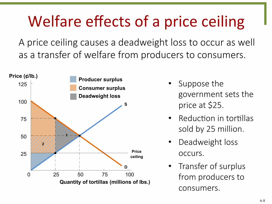
Welfare effects of a price ceiling
Price ceiling
Producer surplus Consumer surplus Deadweight loss
0
25 50 75
100 125
25 50 75 100 Quantity of tortillas (millions of lbs.)
S
D
Price (¢/lb.) • Suppose the
government sets the price at $25.
• Reduc1on in tor1llas sold by 25 million.
• Deadweight loss occurs.
• Transfer of surplus from producers to consumers.
A price ceiling causes a deadweight loss to occur as well as a transfer of welfare from producers to consumers.
2 1

6-9
Welfare effects of a price ceiling • Are price ceilings worth the decrease in total surplus?
– Norma1ve ques1on about which people can disagree. • One way to answer is through studying the alloca1on of
tor1llas. • Because a price ceiling causes a shortage, goods must be
ra1oned. – Ra1oned equally. – First-‐come, first-‐served basis. – Ra1oned to those who are given preference by the government, or to the friends and family of sellers.
• Shortages cause people to engage in rent-‐seeking behavior, such as bribing whoever is in charge of alloca1ng scarce supplies.
6-10
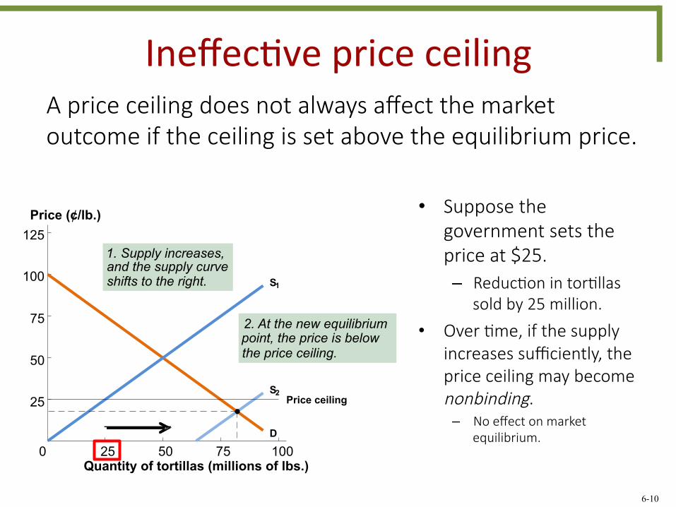
Ineffec7ve price ceiling
1. Supply increases, and the supply curve shifts to the right.
2. At the new equilibrium point, the price is below the price ceiling.
0
25
50
75
100
125
25 50 75 100 Quantity of tortillas (millions of lbs.)
S 1
S 2
D
Price (¢/lb.) • Suppose the government sets the price at $25. – Reduc1on in tor1llas
sold by 25 million.
• Over 1me, if the supply increases sufficiently, the price ceiling may become nonbinding.
– No effect on market equilibrium.
A price ceiling does not always affect the market outcome if the ceiling is set above the equilibrium price.
Price ceiling

6-11
Price floors
0
0 . 5 1 1 . 5 2 2 . 5 3 3 . 5 4 4 . 5
5 1 0 1 5 2 0 2 5 3 0 3 5 Quantity of milk (billions of gals.)
Price ($/gal.)
D
S
0 0 . 5 1 1 . 5 2 2 . 5 3 3 . 5 4 4 . 5
5 1 0 1 5 2 0 2 5 3 0 3 5 Quantity of milk (billions of gals.)
Price ($/gal.)
D
S Excess supply
Price floor Quantity supplied and quantity demanded move in opposite directions.
Suppose the U.S. government imposes a price floor on milk. What effect does this have on the market?
Efficient market with a price of $2.50 per gallon and 15 million gallons of milk being produced.
Inefficient market with a price ceiling set at $3 per gallon and 20 million gallons of milk being produced.
6-12
Price floors • Did the price floor meet the goal of providing support to producers? – Yes. Producers were able to sell some milk at a higher price of $3.00 per gallon.
– No. Some producers may not be able to sell all of their milk because demand no longer meets supply.
• How did the price floor affect welfare? – This ques1on can be answered using the difference in consumer and producer surplus before/a]er government interven1on.

6-13
Welfare effects of a price floor
Price ($/gal.)
Quantity of milk (billions of gals.) 0 0.5 1 1.5 2 2.5 3 3.5 4 4.5
5 10 15 20 25 30 35
Producer surplus S
D
Consumer surplus Deadweight loss
• Suppose the government sets the market price to $3.
• Reduc1on in milk sold by 5 million gallons.
• Deadweight loss occurs (Area 1).
• Transfer of surplus (Area 2) from consumers to producers.
A price floor causes a deadweight loss to occur as well as a transfer of welfare from consumers to producers.
Price floor 2
1

6-14
Welfare effects of a price floor • Are price floors worth the decrease in total surplus? – Norma1ve ques1on about which people can disagree.
• One way to answer is through studying how much excess milk will the government have to buy. – The answer is the en1re amount of excess supply created by the price floor.
– In the above case, 10 billion gallons will be purchased at $3 per gallon.
– The cost to maintain the price floor is then $30 billion.

6-15
Ineffec7ve price floor
0 0 . 5 1
1.5 2
2 . 5 3 3 . 5 4 4 . 5 5 5 . 5 6
5 1 0 1 5 2 0 2 5 3 0 3 5
Price floor
1. Supply decreases, and the supply curve shifts to the left.
Price ($/gal)
Quantity of Milk (billions of gals.)
S 1
D
S 2
2. At the new equilibrium point, the price is above the price ceiling.
• Suppose the government set the price at $3. – Increase in milk sold by
5 million gallons.
• Over 1me, if the supply decreases sufficiently, the price floor may become nonbinding.
– No effect on market equilibrium.
A price floor does not always affect the market outcome if the floor is set below the equilibrium price.

6-16
Ac7ve Learning: Determining market price and quan7ty with price controls
Suppose the government has been convinced to ins1tute a price ceiling on housing rentals for $400 per month. Demand for housing is given as P = 900 – 20Q and supply is P = 40Q, where Q is measured in thousands of housing units.
1. Solve for equilibrium price and quan1ty without a price control.
2. Solve for the price and quan1ty with a price control.
3. Why might a price control may have opposite effects then intended?
6-17
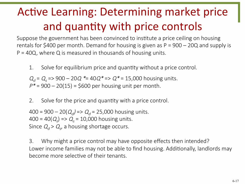
Ac7ve Learning: Determining market price and quan7ty with price controls
Suppose the government has been convinced to ins1tute a price ceiling on housing rentals for $400 per month. Demand for housing is given as P = 900 – 20Q and supply is P = 40Q, where Q is measured in thousands of housing units.
1. Solve for equilibrium price and quan1ty without a price control.
Qd = Qs => 900 – 20Q *= 40Q* => Q* = 15,000 housing units. P* = 900 – 20(15) = $600 per housing unit per month.
2. Solve for the price and quan1ty with a price control.
400 = 900 – 20(Qd) => Qd = 25,000 housing units. 400 = 40(Qs) => Qs = 10,000 housing units. Since Qd > Qs, a housing shortage occurs.
3. Why might a price control may have opposite effects then intended? Lower income families may not be able to find housing. Addi1onally, landlords may become more selec1ve of their tenants.

6-18
Taxes and Subsidies • Price incen1ves can be divided into categories:
– Taxes: Either the buyer or the seller must pay some extra amount to the government on top of the sale price.
• Typically placed on seller. – Subsidies: Either the buyer or the seller receives a payment from the government that lowers the sale price.
• Taxes and subsidies can be used to correct market failures and provide incen1ves or disincen1ves to produce more or less than the equilibrium quan1ty.

6-19
Taxes • Using the case of faQy foods in the U.S., rather than banning them, what would happen if the government taxed them?
• Taxes have two primary effects: – Discourage produc1on and consump1on of the good that is taxed.
– Raise government revenue through the fees paid by those who con1nue buying and selling the good.
• A tax will reduce consump1on and provide a new source of public revenue.

6-20
Effects of a tax paid by the seller
0
2 0
4 0
6 0
8 0
5 1 0 1 5 2 0 2 5 3 0 3 5 4 0 4 5
Price (¢)
Quantity of Whizbangs (millions)
S 2
D
S 1 E 2
E 1 Buyers pay 60¢
Sellers receive 40¢ after the tax
Tax Wedge
• The new supply curve adds $0.20 to all prices, the amount of the tax.
• Taxes drives a wedge between the buyer’s price and the seller’s price.
• The equilibrium quan1ty decreases from 30 million to 25 million.
Suppose the government imposes a $0.20 tax on each unit sold, which the seller must pay. What effect does this have on the market?
6-21
Effects of a tax paid by the seller
0
2 0
4 0
6 0
8 0
5 1 0 1 5 2 0 2 5 3 0 3 5 4 0 4 5
Price (¢)
Quantity of Whizbangs (millions)
Tax $0.20
S 2
E 1 E
S 1
D
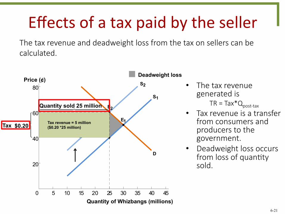
Deadweight loss • The tax revenue
generated is TR = Tax*Qpost-‐tax
• Tax revenue is a transfer from consumers and producers to the government.
• Deadweight loss occurs from loss of quan1ty sold.
The tax revenue and deadweight loss from the tax on sellers can be calculated.
Quantity sold 25 million 2 Tax revenue = 5 million ($0.20 *25 million)
6-22
Ac7ve Learning: Tax revenue and surpluses
Price ($/gal.)
Quantity of milk (billions of gals.) 0 0.5 1 1.5 2 2.5 3 3.5 4 4.5
5 10 15 20 25 30 35
S
D
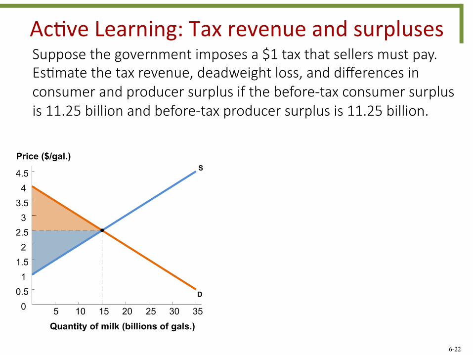
Suppose the government imposes a $1 tax that sellers must pay. Es1mate the tax revenue, deadweight loss, and differences in consumer and producer surplus if the before-‐tax consumer surplus is 11.25 billion and before-‐tax producer surplus is 11.25 billion.

6-23
Ac7ve Learning: Tax revenue and surpluses
Price ($/gal.)
Quantity of milk (billions of gals.) 0 0.5 1 1.5 2 2.5 3 3.5 4 4.5
5 10 15 20 25 30 35
S
D
• TR = $1*10B = $10B • DWL = ½*(15B-‐10B)*(3-‐2)= 2.5B
• Diff(CS) = [($4 – $3)*10B] -‐ 11.25B = -‐1.25B
• Diff(PS) = [($2 – $1)*10B] -‐ 11.25B = -‐1.25B
Suppose the government imposes a $1 tax that sellers must pay. Es1mate the tax revenue, deadweight loss, and differences in consumer and producer surplus if the before-‐tax consumer surplus is 11.25 billion and before-‐tax producer surplus is 11.25 billion.
S + tax

6-24
Effects of a tax paid by the buyer
0
2 0
4 0
6 0
8 0
5 1 0 1 5 2 0 2 5 3 0 3 5 4 0 4 5
Buyers pay 60¢ with 20¢ in taxes
Sellers receive 40¢ E 1
E 2
S
D 1
D 2
Quantity of Whizbangs (millions)
Price (¢)
Tax Wedge
• The new demand curve is $0.20 lower, the amount of the tax.
• Taxes drives a wedge between the buyer’s price and the seller’s price.
• The equilibrium quan1ty decreases from 30 million to 25 million.
Suppose the government imposes a $0.20 tax on each unit sold, which the buyer must pay. What effect does this have on the market?
6-25
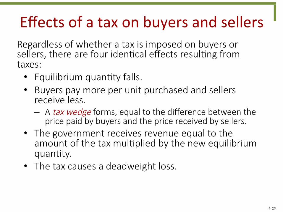
Effects of a tax on buyers and sellers Regardless of whether a tax is imposed on buyers or sellers, there are four iden1cal effects resul1ng from taxes:
• Equilibrium quan1ty falls. • Buyers pay more per unit purchased and sellers receive less. – A tax wedge forms, equal to the difference between the
price paid by buyers and the price received by sellers. • The government receives revenue equal to the amount of the tax mul1plied by the new equilibrium quan1ty.
• The tax causes a deadweight loss.
6-26
Tax incidence
Sellers’ tax burden Buyers’ tax burden
S 2
S 1
D
66
3 0 2 2
46
Buyers pay 66¢, sellers receive 46¢.
Price (¢)
Quantity of Whizbangs (mil.)
S 2
S 1
D 54
3 0 2 2
34
Price (¢)
Quantity of Whizbangs (mil.)
Buyers pay 54¢ sellers receive 34¢
Price (¢) S 2
S 1
D
6 0
3 0 2 5
4 0
Quantity of Whizbangs (mil.)
Buyers pay 60¢ sellers receive 40¢
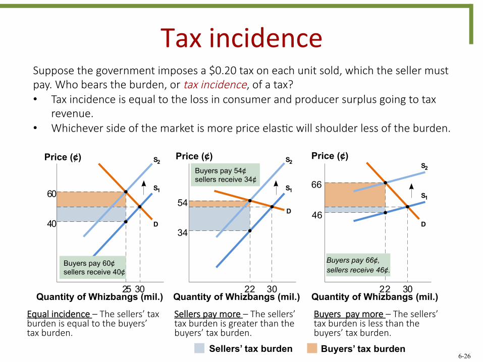
Equal incidence – The sellers’ tax burden is equal to the buyers’ tax burden.
Sellers pay more – The sellers’ tax burden is greater than the buyers’ tax burden.
Buyers pay more – The sellers’ tax burden is less than the buyers’ tax burden.
Suppose the government imposes a $0.20 tax on each unit sold, which the seller must pay. Who bears the burden, or tax incidence, of a tax? • Tax incidence is equal to the loss in consumer and producer surplus going to tax
revenue. • Whichever side of the market is more price elas1c will shoulder less of the burden.
6-27
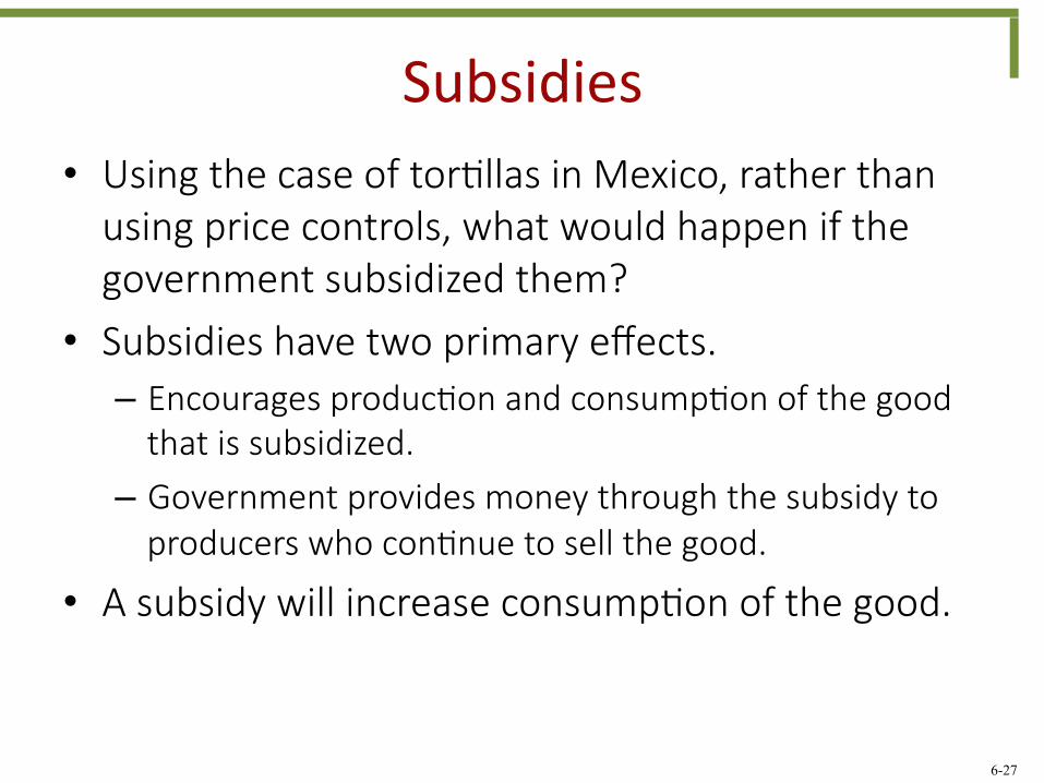
Subsidies • Using the case of tor1llas in Mexico, rather than using price controls, what would happen if the government subsidized them?
• Subsidies have two primary effects. – Encourages produc1on and consump1on of the good that is subsidized.
– Government provides money through the subsidy to producers who con1nue to sell the good.
• A subsidy will increase consump1on of the good.
6-28
Subsidies
D
S 1 S 2
7 0
5 0 6 2
8 8
5 3
Quantity of Tortillas (millions of pounds)
Price (¢/lb.)
E 1 E 2
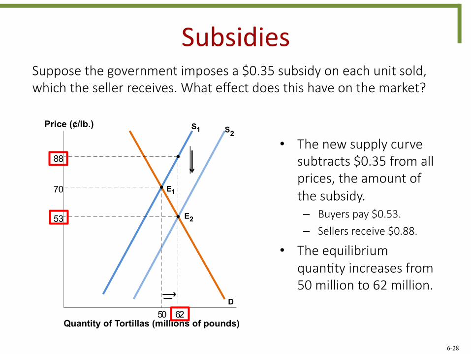
• The new supply curve subtracts $0.35 from all prices, the amount of the subsidy. – Buyers pay $0.53. – Sellers receive $0.88.
• The equilibrium quan1ty increases from 50 million to 62 million.
Suppose the government imposes a $0.35 subsidy on each unit sold, which the seller receives. What effect does this have on the market?

6-29
Government interven7on: A summary
Interven1on Reason for using Effect on price Effect on quan1ty Who gains and who loses? Price floor T o protect producers’
income Price cannot go below the set minimum.
Quan1ty demanded decreases and quan1ty supplied increases, crea1ng excess supply.
Producers who can sell all their goods earn more revenue per item; other producers are stuck with an unwanted excess supply.
Price ceiling T o keep consumer costs low Price cannot go
above the set maximum.
Quan1ty demanded increases and quan1ty supplied decreases, crea1ng a shortage.
Consumers who can buy all the goods they want benefit; other consumers suffer from shortages.
T ax T o discourage an ac1vity or collect money to pay for its consequences; to increase government revenue
Price increases . Equilibrium quan1ty decreases. Government receives increased
revenue; society may gain if the tax decreases socially harmful behavio r . Buyers and sellers of the good that is taxed share the cost. Which group bears more of the burden depends on the price elas1city of supply and demand.
Subsidy T o encourage an ac1vity; to provide benefits to a certain group
Price decreases . Equilibrium quan1ty increases. Buyers purchase more goods
at a lower price. Society may benefit if the subsidy encourages socially beneficial behavior . The government and ul1mately the taxpayers bear the cost.
The following table summarizes the effect of all four government policies analyzed in this chapter.
6-30
How big is the effect of a tax or subsidy?
1
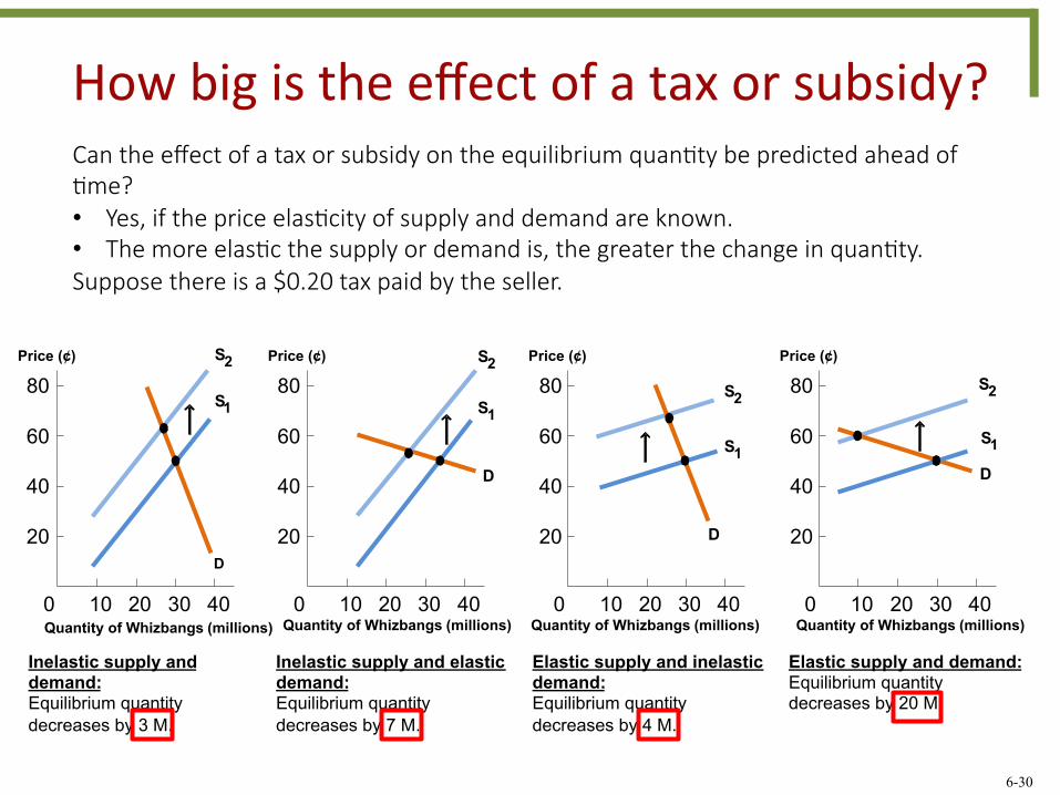
Inelastic supply and demand: Equilibrium quantity decreases by 3 M.
Inelastic supply and elastic demand: Equilibrium quantity decreases by 7 M.
Elastic supply and inelastic demand: Equilibrium quantity decreases by 4 M.
Elastic supply and demand: Equilibrium quantity decreases by 20 M.
Can the effect of a tax or subsidy on the equilibrium quan1ty be predicted ahead of 1me? • Yes, if the price elas1city of supply and demand are known. • The more elas1c the supply or demand is, the greater the change in quan1ty. Suppose there is a $0.20 tax paid by the seller.
0
20 40 60 80
10 20 30 40
Price (¢)
D
S 2 S
Quantity of Whizbangs (millions)
S 1
D
0
20 40 60 80
10 20 30 40
Price (¢) S 2
Quantity of Whizbangs (millions) 0
20 40 60 80
10 20 30 40
Price (¢)
D
S 1
S 2
Quantity of Whizbangs (millions) 0
20 40 60 80
10 20 30 40
Price (¢)
D S 1
S 2
Quantity of Whizbangs (millions)

6-31
Long-‐run versus short-‐run impact
Price ($)
Gasoline (billions of gals.)
Price floor
D D
S
S
Price ($)
Price floor
Gasoline (billions of gals.)
Excess supply Excess supply
The effect of a government interven1on may be lagged. • One example is gasoline and price controls of gasoline. • Because buyers and sellers take 1me to respond to changes in price, some1mes the full
effect of price controls becomes clear only in the long-‐run.
In the short run, driving habits are difficult to change and producers take 1me to increase produc1on. Effect on quan1ty is small.
In the long run, driving habits can be changed and producers can increase produc1on. Effect on quan1ty is large.

6-32
Summary • Basic tools for understanding government interven1ons were introduced: – Price controls (floors and ceilings). – Taxes/subsidies.
• Determining whether the direct supply, demand, or both should shi].