GPS INS Integration SKocaman

8/7/2019 GPS INS Integration SKocaman

http://slidepdf.com/reader/full/gps-ins-integration-skocaman 1/37

ETH Hönggerberg, Zürich

Institute of Geodesy and Photogrammetry

GEODETIC SEMINAR REPORT

GPS and INS Integration with Kalman Filtering

for

Direct Georeferencing of Airborne Imagery

Prepared by:

Sultan Kocaman

Presented to:

Prof. Dr. Hilmar Ingensand

30.01.2003



2

CONTENTS

1 Introduction

2 Fundamentals of the GPS

2.1 Clocks and Time

2.2 GPS Signals

2.3 GPS Receiver

2.4 GPS Observables and Errors

3 Fundamentals of Inertial Navigation

3.1 Basic Concepts of Inertial Navigation3.2 Common Sensor Error Models

3.3 Initialization and Alignment

3.4 System-Level Error Models

4 Kalman Filtering Basics

4.1 Discrete Kalman Filter

4.2 The Extended Kalman Filter

5 GPS and INS Integration

5.1 Integration Modes

5.2 Integration Limitations

6 A Special Application Area: Direct Georeferencing of Airborne Imagery

7 Conclusions and Future Work

REFERENCES

APPENDIX

Random Processes: Basic Concepts



3

1 INTRODUCTION

Georeferencing can be defined as a process of obtaining knowledge about the origin of some event

in space-time. Depending on the sensor type, this origin needs to be defined by a number of

parameters such as time, position (location), attitude (orientation) and possibly also the velocity of

the object of the interest. When this information is attained directly by means of measurements

from sensors on-board the vehicle the term direct georeferencing is used [Skaloud, 1999].

For georeferencing the image data, the position (X0, Y0, Z0) and orientation (ω, ϕ, κ) of the sensor,

which also are called as exterior orientation elements, should be known. Then, the uncorrected

image vector is transformed to the corrected georeferenced position and the relation between the

local image coordinate system and the global object frame is solved. The traditional way of

georeferencing of airborne imagery is to use ground control points (GCPs) which counts a major

cost for photogrammetry projects. A number of different vehicles and methods can be used for

direct georeferencing of airborne imagery depending on the sensor and platform type. Today,

differential kinematic GPS positioning is a standard tool for determining the camera exposure

centres for aerial triangulation [Heipke et al, 2002]. Airborne GPS can greatly reduce, but not

completely eliminate the need for ground control.

Since the need for GCP and overlapping imagery cannot be eliminated with the use of GPS, theintegration of GPS and the inertial technology became a subject of research in this field. Inertial

navigation relies on knowing the initial position of the object, velocity and attitude, and thereafter

measuring the attitude rates and accelerations. An Inertial Navigation System (INS) consists of an

Inertial Measurement Unit (IMU) or Inertial Reference Unit (IRU), and navigation computers to

calculate the gravitational acceleration. However, in this report, the terms INS and IMU are used

for the same purpose. An IMU is composed of gyroscopes, which is used for determining the

rotation elements of the exterior orientation, and accelerometers, which provides the sensor

velocity and position. In this report, use of the term INS is preferred. In principle, a GPS/IMU

sensor combination can yield the exterior orientation elements of each image without aerial

triangulation.

The application of direct georeferencing to the image data provides some important advantages,

which can be summarized as:

♦ Direct georeferencing enables a faster acquisition of the exterior orientation, since the

computational burden for automatic aerial triangulation is higher compared to the effort for

GPS/inertial integration [Cramer, 1999].



4

♦ Direct georeferencing removes limitations to the flight path during image acquisition.

Continuous absolute GPS trajectories, as obtainable by on-the-fly (OTF) methods, would in

principle permit an aerial triangulation without ground control points. For that purpose a

certain number of images has to be captured in the well-known photogrammetric block

configuration. However, this flight configuration can be disadvantageous, if only small areas

have to be captured or if a linear flight path is aspired for tasks like the supervision of power

lines or the image acquisition at coast lines [Cramer, 1999].

♦ Additional problems of image matching required for automatic aerial triangulation are avoided

if direct georeferencing is applied [Cramer, 1999].

Integrated systems will provide a system that has superior performance in comparison with either a

GPS, an INS, or vision-based stand-alone system. The main strengths and weakness of INS and

DGPS are summarized in figure 1.1.

Figure 1.1: Benefits of INS/DGPS Integration [Skaloud, 1999].

The overall performance of the direct orientation method is limited primarily by the following

components:

♦ Quality of the calibration of the integrated system:

INS

! high position velocity accuracy over

the short term

! accurate attitude information

! accuracy decreasing with time

! high measurement output rate

! autonomous! no signal outages! affected by gravity

DGPS

! high position velocity accuracy over

the long term

! noisy attitude information (multiple

antenna arrays)

! uniform accuracy, independent of

time

! low measurement output rate

! non-autonomous! cycle slip and loss of lock

! not sensitive to gravity

INS/DGPS

! high position and velocity accuracy

! precise attitude determination

! high data rate

! navigational output during GPS signal

outages

! cycle slip detection and correction

! gravity vector determination



5

− Imaging sensor modeling

− Lever arm between INS and GPS antenna

− Boresight transformation between INS and camera frames

♦ In-flight variation of the calibration components

♦ Rigidity of the imaging sensor/INS mount

♦ Quality of the IMU sensor

♦ Continuity of the GPS lock

♦ Kalman filter design [Grejner-Brzezinska, Toth, 2000].

Before using the position and orientation components (GPS antenna and IMU) for sensor

orientation, we must determine the correct time, spatial eccentricity, and boresight alignment

between the camera coordinate frame and IMU. The calibration of the GPS/IMU and the camera isvital since minor errors will cause major inaccuracies in object point determination [Sanchez,

Hothem]. Direct georeferencing of airborne imaging data by INS/DGPS is schematically depicted

in figure 1.2.

Figure 1.2: Direct georeferencing of airborne imaging by INS/DGPS [Skaloud, 1999].



6

Kalman Filter is an extremely effective and versatile procedure for combining noisy sensor outputs

to estimate the state of a system with uncertain dynamics. In GPS/INS integration case, noisy

sensors include GPS receivers and IMU components, and the system state include the position,

velocity, acceleration, attitude, and attitude rate of a vehicle. Uncertain dynamics include

unpredictable disturbances of the host vehicle and unpredictable changes in the sensor parameters

[Grewal et al., 2001]. Kalman filter optimally estimates position, velocity, and attitude errors, as

well as errors in the inertial and GPS measurements [Grejner-Brzezinska and Toth, 1998].

Main purposes of this report are to figure out basic system requirements of direct georeferencing of

airborne imagery using GPS and INS, to explain the fundamentals of GPS/INS integration with

Kalman Filtering and limitations of the integration, and to describe the common problems and

results reported in the literature.

In the second and third parts of this report, the fundamentals and basic error models of GPS and

INS are introduced, respectively. The theory of Kalman filtering for discrete and continuous

processes are explained in the fourth part. While the integration purposes and types of GPS and

INS are provided in the fifth part, a general overview of the applications seen in the literature is

given in sixth part. The conclusion and future work is placed at the and of this report.



7

2 FUNDAMENTALS of the GPS

The GPS, officially also known as NAVSTAR (Navigation and Satellite Timing and Ranging), is

part of a satellite-based navigation system developed by the U.S. Department of Defense. GPS

belongs to a large class of radio navigation systems that allow the user to determine his range

and/or direction from a known signal transmitting station by measuring the differential time of

travel of the signal. The Global Orbiting Navigation Satellite System (GLONASS) developed by

Russia has almost an equivalent structure and used for satellite radio navigation purposes similar to

GPS. Terrestial radio navigation systems predate the satellite systems and include such as VOR

(VHF Omnidirectional Range) and DME (Distance Measuring Equipment) for civilian aviation; the

military equivalent, Tacan (Tactical Air Navigation); and low-frequency, long-range systems such

as LORAN (Long Range Navigation) and OMEGA (Jekeli, 2000).

The GPS comprises a set of orbiting satellites at known locations in space and their signals can be

observed on the Earth. Three distances to distinct satellites having known positions provide

sufficient information to solve the observer’s three-dimensional position. The system is designed so

that a minimum of four satellites is always in view anywhere in the world to provide continual

positioning capability. This is accomplished with 24 satellites distributed unevenly in six

symmetrically arranged orbital planes.

The applications of GPS range from military navigation, vehicle monitoring, to sporting activities.

For geodetic applications, the precise measurement of baselines (relative positioning) in static

mode of GPS is widely used. Static positioning involves placing the receiver at a fixed location on

the Earth and determining the position of that point. Opposite to this, kinematic positioning refers

to determining the position of a vehicle or a platform that is moving continually with respect to

Earth. It is also known as real-time positioning. The term navigation is used for real-time

processing of the positioning data. Differential GPS (DGPS) is a technique for reducing the error in

GPS-derived positions by using additional data from a reference GPS receiver at a known position.The most common form of DGPS involves determining the combined effects of navigation

message ephemeris and satellite clock errors at a reference station and transmitting the pseudorange

corrections in real time, to a user’s receiver (Grewal et al., 2001).

The GPS is not without problems and limitations (Jekeli, 2000). It is not a self-contained,

autonomous system. The user must be able to “see” the GPS satellites. Satellite visibility may be

obstructed locally by intervening buildings, mountains, bridges, tunnels, etc. For kinematic

applications, the effects of electronic interference or brief obstructions may cause the receiver to

miss one or more cycles of the carrier wave. The frequency of the data output in most receivers is



8

often 1 Hz. Most of the error in GPS positioning come from medium propagation effects that are

unpredictable to model such as atmospheric effects.

2.1 Clocks and Time

Each GPS satellite carries an atomic clock to provide timing information for the signals transmitted

by the satellites. The clocks are oscillating at a particular frequency. The relationship between the

phase φ , frequency ƒ, and the time is:

ƒ(t )=dt

t d )(φ (2.1)

where t represents true time. The phase of an oscillating signal is the angle it sweeps out over time

(0≤φ≤2π) and has the units of cycle. The frequency of the signal is the rate at which the phase

changes in time and has the units of Hertz (cycles per second).

∫ ƒ+=t

t o

dt t t t ')'()()( 0φ φ (2.2)

t0 is some initial time. τ denote the indicated time related to the phase:

τ(t )=0

)0)((

f

t φ φ −(2.3)

ƒ0 is some nominal (constant) frequency since the initial indicated time does not coincide with

initial phase (φ (t 0) ≠ φ 0 ).

The oscillator clock time (τ) and the true time (t ) differ from each other both in scale and in origin.

The true time reflects the atomic clock time in U.S., which also differs from Coordinated Universal

Time (UTC) by 2000 with 13 seconds. However, the GPS true time is calibrated by U.S. atomic

time. The true time reflects the fact that the times indicated on satellite and receiver clocks are not

perfectly uniform and must be calibrated by master clocks on the Earth. The relationship between

the phase-time, τ, and the true time, t, is:

τ(t )=t - t 0 + τ(t 0) + δ τ(t ), (2.4)

where,

∫ ƒƒ=

t

t o

dt t t ')'(1

)(0

δ δ

The abbreviated form of (2.4) is:

τ(t )=t -∆ τ(t) (2.5)



9

2.2 GPS Signals

The signal is a carrier wave (sinusoidal wave) modulated in phase by binary codes that represent

interpretable data. It can be represented mathematically by:

S(t)= AC(t)D(t)cos(2πƒt) (2.6)

where ƒ is the frequency of the carrier wave, and A is the amplitude of the signal. The code

sequence C(t) is a step function having values (1, -1), also known as chips or bits. D(t) represents a

data message.

Each satellite actually transmits two different codes, the C/A (coarse acquisition) code and the P-

code (precision code). The P-code has 10 times higher chipping rate and wavelength in comparison

with C/A code. They are transmitted on two separate microwave regions, an L1 signal with carrier

frequency ƒ1 = 1545.72 MHz and with wavelength λ1=0.1903 m; and an L2 signal with carrier

frequency ƒ2 = 1227.6 MHz and with wavelength λ2=0.2442 m. The transmission on two

frequencies allows approximate computation of the delay of the signal due to ionospheric

refraction. The total signal transmitted by the satellite is given by the sum of three sinusoids, two

for the two codes on the L1 carrier and one for the P-code on the L2 carrier. The total signal

transmitted by a GPS satellite is given by

SP(t)=APP

P(t)W

P(t) D

P(t)cos(2πƒ1t) + ACC

P(t) D

P(t)sin(2πƒ1t) + BPP

P(t)W

P(t)D

P(t)sin(2πƒ2t) (2.7)

AP, AC, and BP represent amplitudes of the corresponding codes, C and P represent C/A and P

codes, D represents the data message, superscript P identifies a particular satellite, and W represents

a special code which is used to decrypt a military code.

The codes serve two operational purposes: determining the range between the satellite and receiver

and to spread the signal over a large frequency bandwidth, thus permitting small antennas on the

Earth to gather the transmitted signal. Both codes consist of unique sequences of binary states that

are generated using a pseudorandom noise (PRN) algorithmic process. The PRN for C/A code is

different for each satellite and repeats every millisecond. For P-code, it is much longer and repeats

only after 38 weeks. Each satellite uses only one distinct week’s worth of the code. The satellites

are distinguished by the codes rather than by frequency.



10

2.3 GPS Receiver

Before the signal is processed by the receiver, it is pre-amplified and filtered at the antenna, and

subsequently down-shifted in frequency to a more manageable level for processing (Jekeli, 2000).

The mixed signal is given by

Sr(t) SP(t)=A cos(2πƒLOt) cos(2πƒSt + φ(t))

=2

Acos(2π(ƒS-ƒLO)t + φ(t)) +

2

Acos(2π(ƒS+ƒLO)t + φ(t)) (2.8)

where Sr(t) is the pure signal sinusoid generated by the receiver oscillator, ƒLO is the local oscillator

frequency, SP(t) is the satellite signal with frequency ƒS, and A is an amplitude factor.

The satellite signal is then shifted to an intermediate frequency (IF), and appropriate filters are

applied to control the amplitude of the signal for subsequent processing. The signal then passes to

the main signal processing part of the receiver.

To calculate the distance between the satellite and the receiver, the time tag of the signal at the time

of transmission and the time of reception at the receiver is compared, and using the speed of the

light, the delay is converted to the distance. It is not the true range if the satellite and the receiverclocks differ; and therefore, the calculated range is called pseudorange.

2.4 GPS Observables and Errors

A broad overview of GPS errors is provided in table 2.1. The largest error is due to the receiver

clock. The next significant error source is the medium in which the signal must travel. This

includes the Ionosphere, which has an altitude between 50 km to 1000 km and has many free

electrons; and the Troposphere, which is a non-dispersive medium and contains mostly electrically

neutral particles.

Table 2.1: Error sources in GPS positioning (Jekeli, 2000).

Error Source Typical Magnitude

Receiver clock error (synchronized) 1 µs (300 m)

Residual satellite clock error 20 ns (6m)

Satellite synchronization to UTC 100 ns (30 m)

Selective Availability (cancelled by 2001) 100 m



11

Orbit error (precise, IGS) 20 cm

Tropospheric delay <30 m

Ionospheric delay <150 m

Multipath <5 m (P-code); <5 cm (phase)

Receiver Noise 1 m (C/A code); 0.1 m (P-code); 0.2 mm (L1 phase)

Other errors in GPS observables include the multipath error (the reflection of the GPS signal from

nearby objects prior to entering the antenna), equipment delays and biases, antenna eccentricities

(phase center variations), and the thermal noise of the receiver.

The pseudorange is formulated as

SrP(τr)=ρr

P(τr) + c( ∆ τr(t) - ∆ τP

(t-∆ trP)) + ∆ ρP

iono,r+ εP

p,r(2.9)

where ρrP(τr) is the true range between the satellite and the receiver, ∆ tr

Pis the time of transit,

∆ ρP

iono,ris the ionospheric error for each satellite, c is the speed of the light, and εP

p,rrepresents

pseudorange observation error (different for each satellite). For simplicity, the Tropospheric delay,

the equipment and antenna offsets, the multipath error, and the time registration error due to the

receiver clock error are excluded.

The phase observable can be expressed as follows:

φrP(τr)=

c

f 0ρr

P(τr) + 0 f (∆ τr(t) - ∆ τP

(t-∆ trP)) + φ0,r - φ0

P– Nr

P+ ∆ φP

iono,r+ εP

φ ,r(2.10)

where φ0,r and φ0P

are the arbitrary phase offsets NrP

is the integer representing the unknown

number of full cycles and also called as carrier phase ambiguity, εP

φ ,ris the phase observation error.



12

3 FUNDAMENTALS of INERTIAL NAVIGATION

3.1 Basic Concepts of Inertial Navigation

Inertia is the propensity of bodies to maintain constant translational and rotational velocity, unless

disturbed by forces or torques, respectively (Newton’s first law of motion). An inertial reference

frame is a coordinate frame which Newton’s law of motion are valid. Inertial reference frames are

neither rotating nor accelerating (Grewal et al., 2001). Inertial sensors measure rotation rate and

acceleration by gyroscopes and accelerometers respectively. Accelerometers cannot measure

gravitational acceleration, which is an accelerometer in free fall or in orbit has no detectable input.

The input axis of an inertial sensor defines which vector component it measures. Multiaxis sensors

measure more than one component.

Inertial navigation uses gyroscopes and accelerometers to maintain an estimate of the position,

velocity, attitude, and attitude rates of the vehicle in or on which the INS is carried. An INS

consists of navigation computers, to calculate the gravitational acceleration and to integrate the net

acceleration, and an inertial measurement unit containing accelerometers and gyroscopes.

Literally, there are thousands of designs for gyroscopes and accelerometers. Not all of them are

used for inertial navigation. For example, gyroscopes are used for steering and stabilizing ships,missiles, cameras and binoculars, etc. The acceleration sensors are also used for measuring gravity,

sensing seismic signals, leveling, and measuring vibrations.

Traditionally, inertial systems have been divided into three groups according to the free-running

growth of their position error (Skaloud, 1999):

• the strategic-grade instruments ( performance ≈ 100 ft/h)

• the navigation-grade instruments (performance ≈ 1 nm/h)

• the tactical-grade instruments (performance ≈ 10-20 nm/h)

In a further categorization, the inertial navigation systems are designed in two main groups: the

platform (or gimbaled ) systems and the strapdown systems. In a gimbaled system the

accelerometer triad is rigidly mounted on the inner gimbal of three gyros (see figure 3.1.b). The

inner gimbal is isolated from the vehicle rotations and its attitude remains constant in a desired

orientation in space during the motion of the system. The gyroscopes on the stable platform are

used to sense any rotation of the platform, and their outputs are used in servo feedback loops with

gimbal pivot torque actuators to control the gimbals such that the platform remains stable. These



13

systems are very accurate, because the sensors can be designed for very precise measurements in a

small measurement range.

In contrary, a strap-down inertial navigation system uses orthogonal accelerometers and gyro triads

rigidly fixed to the axes of the moving vehicle (figure 3.1.a). The angular motion of the system is

continuously measured using the rate sensors. The accelerometers do not remain stable in space,

but follow the motion of the vehicle.

Figure 3.1: Inertial measurement units (Grewal et al., 2001).

3.2 Common Sensor Error Models

Gyroscopes, which are used as attitude sensors in inertial navigation, are also called as inertial

grade. There are many types of gyroscope designs, such as momentum wheels, rotating

multisensor, laser gyroscopes, etc. Error models for gyroscopes are primarily used for twopurposes: predicting performance characteristics as function of gyroscope design parameters and

calibration and compensation of output errors. The common error sources for gyroscopes are output

bias, input axis misalignments, combined (clustered) three-gyroscope compensation, input/output

non-linearity, and acceleration sensitivity.

Depending on the purpose, acceleration sensors also have several designs such as, gyroscopic

accelerometers, pendulous accelerometers, strain-sensing accelerometers, etc. The main error

sources for accelerometers are biases, parameter instabilities (i.e., turn-on and drift), centrifugal



14

acceleration effects due to high rotation rates, center of percussion, and angular accelerometer

sensitivity.

3.3 Initialization and Alignment

INS initialization is the process of determining initial values for system position, velocity, and

attitude in navigation coordinates. INS position initialization ordinarily relies on external sources

such as GPS or manual entry. INS velocity initialization can be accomplished by starting when it is

zero (i.e., the host vehicle is not moving) or by reference to the carrier velocity.

INS alignment is the process of aligning the stable platform axes parallel to navigation coordinates

(for gimbaled systems) or that of determining the initial values of the coordinate transformation

from sensor coordinates to navigation coordinates (for strapdown systems). There are four basic

methods for INS alignment (Grewal et al., 2001):

i) Optical alignment using either optical line-of-sight reference to a ground based direction or an

on board star tracker.

ii) Gyrocompass alignment of stationary vehicles, using the sensed direction of acceleration to

determine the local vertical and sensed direction of rotation to determine north.

iii) Transfer alignment in a moving host vehicle, using velocity matching with an aligned and

operating INS.

iv) GPS-aided alignment, using position matching with GPS to estimate the alignment variables.

3.4 System-Level Error Models

Since there is no single, standard design for an INS, the system-level error sources vary very much.

General error sources can be classified as:

i) initialization errors, comes from initial estimates of position and velocity;

ii) alignment errors, from period for initial alignment of gimbals or attitude direction cosines (forstrapdown systems) with respect to navigation axes;

iii) sensor compensation errors, occur due to the change in the initial sensor calibration over the

time;

iv) gravity model errors, is the influence of the unknown gravity modeling errors on vehicle

dynamics.



15

4 KALMAN FILTERING BASICS

Within the significant toolbox of mathematical tools that can be used for stochastic estimation from

noisy sensor measurements, one of the most well known and often-used tools is what is known as

the Kalman Filter . The Kalman filter is named after Rudolph E. Kalman, who in 1960 published

his famous paper describing a recursive solution to the discrete-data linear filtering problem

(Kalman, 1960). The Kalman Filter is essentially a set of mathematical equations that implement a

predictor-corrector type estimator that is optimal in the sense that it minimizes the estimated error

covariance—when some presumed conditions are met. Since the time of its introduction, the

Kalman Filter has been the subject of extensive research and application, particularly in the area of

autonomous or assisted navigation.

Basically, Kalman Filter is a special case of sequential least square estimation, where initial

measurement is equal to the first measurement and design matrix of the second position is an

identity matrix. Kalman Filter also takes the velocity as an unknown parameter. Three sequential

algorithms; Triangular Factor Update (TFU) with Gauss/Cholesky decompositions, Givens Update

and Kalman Update for photogrammetric processing of images were emphasized by Gruen (1984)

and Gruen and Kersten (1992). For more detailed information on least squares filtering of dynamic

linear systems and Kalman filtering, see Gelb (1974), and Salzmann (1993).

4.1 Discrete Kalman Filter

Basic concepts of random processes can be found in the appendix. The Kalman Filter addresses the

general problem of trying to estimate the state x∈ℜnof a discrete-time controlled process that is

governed by the linear stochastic difference equation

xk =Axk-1 +Buk + wk-1 (4.1)

with a measurement z∈ℜm that is

zk =Hxk + vk (4.2)

The random variables wk and vk represent the process and measurement noise (respectively). They

are assumed to be independent (of each other), white, and with normal probability distributions

p(w)~N (0,Q)

p(v)~N (0,R)

In practice, A, the process noise covariance Q, and measurement noise covariance R matrices

might change with each time step. However, here, they are assumed to be constant.

(4.3)

(4.4)



16

Let’s define x k-∈ℜn

as a priori state estimate at step k given the knowledge of the process prior to

step k, and x k∈ℜnas a posteriori state estimate at step k given the measurement zk . A priori and a

posteriori estimate errors and error covariances are:

ek-

≡ xk - x k

-

, Pk

-

=E[ek-

ek-T

]

ek≡ xk - x k , Pk=E[ek ekT]

The linear combination between a posteriori state estimate x k , a priori state estimate x k- , and a

weighted difference between an actual measurement zk and measurement prediction H x k- is:

x k = x k

-

+ K(zk - H x k- ) (4.5)

In the equation, (zk - H x k- ) is called measurement innovation or the residual. K matrix is also

called as Kalman gain matrix and can be shown as:

K k = Pk

-

H T (H Pk

-

H T + R)-1 (4.6)

The Kalman Filter estimates a process by using a form of feedback control: the filter estimates the

process state at some time and then obtains feedback in the form of (noisy) measurements. As such,

the equations for the Kalman Filter fall into two groups: time update equations and measurement

update equations. The time update equations are responsible for projecting forward (in time) the

current state and error covariance estimates to obtain the a priori estimates for the next time step.

The measurement update equations are responsible for the feedback—i.e. for incorporating a new

measurement into the a priori estimate to obtain an improved a posteriori estimate (Welch and

Bishop, 2002). After each time and measurement update pair, the process is repeated with theprevious a posteriori estimates used to project or predict the new a priori estimates in recursive

nature (figure 4.1).

Figure 4.1: A complete picture of the Kalman Filter (Welch and Bishop, 2002).



17

4.2 The Extended Kalman Filter

Extended Kalman Filter (EKF) linearizes the current mean and covariance when the process to be

estimated or the related measurement is non-linear. The stochastic difference equation of the state

vector x∈ℜn of the non-linear process is defined as:

xk = ƒ( xk-1 , uk , wk-1) (4.7)

with a measurement z∈ℜmthat is

zk = h(xk , vk ) (4.8)

where the random variables wk , and vk represent the process and measurement noise. We can

approximate the state and measurement vectors as:

x~ k = ƒ( x k-1 , uk , 0) (4.9)

z

~k = h( x

~k , 0) (4.10)

where x k is a posteriori estimate of the state. The actual state and measurement vectors related with

the approximated state and measurement vectors are:

xk ≈ x~ k +A(x k-1 - x k-1) + Ww k-1 (4.11)

zk ≈ z~ k +H(x k - x~ k ) + Vv k (4.12)

where;

][

][],[

j

ik ji

x

f A

δ

δ = ( x k-1 , uk , 0) (4.13)

][

][],[

j

ik ji

w

f W

δ

δ = ( x k-1 , uk , 0) (4.14)

][

][],[

j

ik ji

x

h H

δ

δ = ( x~ k , , 0) (4.15)

][

][],[

j

ik ji

v

hV

δ

δ = ( x~ k , , 0) (4.16)

The definitions of the prediction error and measurement residual are respectively:

e~ xk ≡ xk - x~ k ≈ A(x k-1 - x k-1) + εk (4.17)

e~ zk ≡ zk - z~ k ≈ H e~ xk

+ ηk (4.18)

where εk and ηk represent new independent random variables having zero mean and covariance

matrices and , with and as in WQW T and VRV T

, with Q and R as in (4.3) and (4.4) respectively.

The equations (4.17) and (4.18) are linear, and they are similar to the equations (4.1) and (4.2) from

Discrete Kalman Filter. A second (hypothetical) Kalman Filter can be used with the actual

measurement residual e~

zk in equation (4.18) and the prediction error to e xk given by equation



18

(4.17) to estimate e k which can be used to obtain the a posteriori estimates for the original non-

linear process as:

x k = x~ k + e k (4.19)

The random variables of equations (4.17) and (4.18) have approximately following probability

distributions:

p( e~ xk ) ~ N(0, E[ e~ xk

e~ xk

T

])

p(εk ) ~ N(0, WQk W T )

p(ηk ) ~ N(0, VRk V T )

Given these approximations and letting the predicted value of e k be zero, the Kalman Filter

equation used to estimate e k is:

e k = Kk e~

zk (4.20)

By substituting equation (4.20) back into equation (4.19) and making use of equation (4.18) we get:

x k = x~ k + Kk e~

zk

= x~ k + Kk ( zk - z~ k ) (4.21)

Equation (4.21) now can be used for the measurement update in the extended Kalman Filter. A

complete set of EKF equations is shown in figure 4.2. The term x~ k is substituted with x k

-

to be

consistent with Discrete Kalman Filter equations.

Figure 4.2: A complete picture of the operation of the extended Kalman filter (Welch and Bishop,

2002).



19

5 GPS and INS INTEGRATION

The Galileo’s Law, δ x= 0.5δ at 2, illustrates the position prediction precision of a moving platform,

where δ x, δ a, and t represent variation in position, change in acceleration, and the time interval

respectively. The relatively low data output rate of GPS receivers (usually 1 Hz) might not meet the

cm level accuracy requirements of aerial photogrammetry. This problem becomes more serious

when the potential temporarily loss of a GPS signal occurs or phase ambiguity resulting from cycle

slips considered. INS provides the dynamics of motion between GPS epochs at high temporal

resolution and complements the discrete nature of GPS in the occurance of cycle slips or signal

loss.

In addition, positioning with INS requires the integration with respect to time of accelerations and

angular rates, the measurement noise accumulates and results in long wavelength errors. GPS

errors do not accumulate, but in short term, they are relatively larger and the measurements have

poorer resolution. INS is an autonomous system, except the initialization requirements, and do not

ask for external support.

Due to the complementary nature of both system, the integrated GPS/INS has become widely used

positioning purposes, especially on mobile mapping systems. The integrated systems are in use on

different platforms, such as aircrafts, ground vehicles, satellites, etc. Several systems have beendeveloped around the world.

When the navigation information is provided by an integrated INS/DGPS system, the equation of

direct georeferencing for aerial frame cameras takes the form:

r im

= r mins/dgps (t) + Rbm(t)[si Rc

b r ic(t) + ab

] (5.1)

where,

r im

is coordinate vector of a specific point (i) in the mapping frame,

r m

ins/dgps (t) is coordinate vector of INS center in the mapping frame, determined by INS/DGPS

integration,

Rbm(t) is the attitude matrix from INS body frame to the mapping frame, , determined by

INS/DGPS integration,

si is a scale factor between the image and mapping coordinate frames for a specific point (i),

usually determined by processing the captured imagery in stereo pairs,

Rcb

is the rotation matrix (orientation offset) between the camera frame and the INS body frame

determined from calibration,

r ic(t) is the vector of coordinates (i.e., x, y, -f) observed in the image frame for a specific image (t)

and point (i),



20

abis the vector of the translation offset between the INS and the camera centre in the INS body

frame determined by terrestrial measurements as part of the calibration process (Skaloud, 1999).

However, some small changes should be done in this equation when pushbroom cameras or other

applications such SAR are considered. For SAR applications, see Dowman (1995) for laser

applications see Favey et al. (1999).

5.1 Integration Modes

The types of integration can be categorized by the extent to which data from each component aid

the other’s function. First one is coupling of the systems and depends on the mechanization or the

architecture of the system. The second categorization parameter is by the method of combining or

fusing the data to obtain position coordinates.

The system mechanization is generally understood in two ways, tight coupling and loosely

coupling; where no coupling implies no data feedback from either instrument to the other for the

purpose of improving ist performance. Tightly coupled sensors are treated as belonging to a single

system producing complementary types of data. The produced data are produced simultaneously

and optimally, and used to enhance the function of of individual sensor components where

possible. In a loosely coupled system, processed data from one instrument are fed back in an aiding

capacity to improve the utility of the other’s performance, but each instrument still has ist own

individual data processing algorithm.

The real-time feedback of INS velocities to the GPS receiver enables an accurate prediction of GPS

pseudorange and phase at next epoch, thus allowing a smaller bandwidth of the receiver tracking

loop in a high-dynamic environment with a subsequent increase in accuracy. Conversely, inertial

navigation improves if the GPS solution functions as an update in a Kalman filter estimation of the

systematic errors in the inertial sensors. Similarly, GPS positions and velocities may be used to aidthe INS solution in a high-dynamic situation by providing a better reference for propagating error

states based on the linear approximation. (Jekeli, 2000)

There are two basic categories of processing algorithms that are centralized and de-centralized. In

centralized processing, the raw sensor data is are combined optimally using one central processor

to obtain a position solution. This kind of processing is usually associated with tight system

integration. Decentralized processing is a sequential approach to processing, where processors of

individual systems provide solutions that subsequently are combined with various degrees of

optimality by a master processor. In principle, if the statistics of the errors are correctly propogated,



21

the optimal decentralized and centralized methods should yield identical solutions (Jekeli, 2000). In

some certain cases, such as system fault detection, isolation, and correction capability and the

relative computational simplicity makes the decentralized approach more favourable. The

centralized approach provides the best performance in navigation solutions that a single robust

Kalman filter model. Different forms of integration are evaluated in table 5.1.

Table 5.1: Different forms of Kalman filter implementation (Skaloud, 1999).

Implementation Advantages Disadvantages

Open loop • KF may be run external to INS,

suitable for platform INS

• Used when only navigation solution

from INS available

• Non-linear error model due to

large second-order effect

• Extended KF needed

Closed loop • Inertial system errors, linear model

is sufficient

• Suitable for integration at softwarelevel

• More complex processing

• Blunders in GPS may affect INS

performance

Loosely coupled

(decentralized)

• Flexible, modular combination

• Small KF, faster processing

• Suitable for parallel processing

• Sub-optimal performance

• Unrealistic covariance

• Four satellites needed for a stable

solution

• INS data not used for ambiguity

estimation

Tightly-coupled

(centralized)

• One error state model

• Optimal solution

• GPS measurements can be used

with less than 4 satellites• Direct INS aiding throughout GPS

outages

• Faster ambiguity estimation.

• Large size of error state model

• More complex processing

The vector state estimation can be implemented in open or closed, whether the estimated sensor

errors are fed back to correct the measurements. When properly designed, the closed-loop

implementation generally has better performance and is therefore the preferred implementation

when using a strapdown INS. The loosely-coupled filtering approach has been highly popular due

its modularity and smaller filter size. Although the arguments for choosing either form of the

implementation have been very balanced, the tightly-coupled approach is currently gaining more

weight mainly due to the rapid increase in computational power (Skaloud, 1999).

5.2 Integration Limitations

The performance of an integrated INS/DGPS is a complex process depending on a variety of

parameters including

• quality and type of inertial sensors• the baseline length



22

• operational aspects

• the validity of error models

• the estimation algorithm. (Skaloud, 1999)

The improvements in trajectory determination are usually sought in the development of better

models and estimation algorithms. With the rapid increase of computational power, the trend of

finding the most suitable error model for a specific system and specific conditions is being replaced

by using a multi-model approach in conjunction with some type of adaptive estimation. Another

limiting factor band frequency. In the lower frequencies, the INS/DGPS integration reduces the

overall error; and in the high frequencies, the overall error is not reduced (Skaloud, 1999).



23

6 A SPECIAL APPLICATION AREA: DIRECT GEOREFERENCING of

AIRBORNE IMAGERY

In the literature, there are several system designs for georeferencing of airborne images; and

regarding to these designs, different integration methods are proposed. In general, strapdown INSs

are preferred due to its low-cost character. The trend is tending to implementation of integration

methods for low-cost IMU and most of the applications are in this manner. However, different

systems ask for different accuracies. A brief overview of accuracy requirements for different

applications areas can be found in Schwarz et al (1994), and Schwarz (1995).

In the University of Calgary the INS/GPS integration strategies are analyzed and different design

methods for several system implemetations are suggested. The results of two different

implementations, a low-cost system and a high-cost navigation grade system, using strapdown

INSs are presented by Schwarz (1995). Error models for INS/GPS integration and design methods

for improving attitude accuracy are discussed by Skaloud and Schwarz (2000).

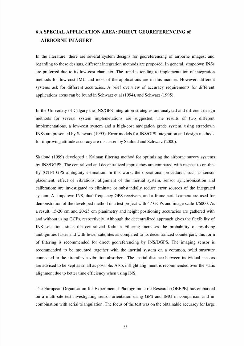
Skaloud (1999) developed a Kalman filtering method for optimizing the airborne survey systems

by INS/DGPS. The centralized and decentralized approaches are compared with respect to on-the-

fly (OTF) GPS ambiguity estimation. In this work, the operational procedures; such as sensor

placement, effect of vibrations, alignment of the inertial system, sensor synchronization andcalibration; are investigated to eliminate or substantially reduce error sources of the integrated

system. A strapdown INS, dual frequency GPS receivers, and a frame aerial camera are used for

demonstration of the developed method in a test project with 47 GCPs and image scale 1/6000. As

a result, 15-20 cm and 20-25 cm planimetry and height positioning accuracies are gathered with

and without using GCPs, respectively. Although the decentralized approach gives the flexibility of

INS selection, since the centralized Kalman Filtering increases the probability of resolving

ambiguities faster and with fewer satellites as compared to its decentralized counterpart, this form

of filtering is recommended for direct georeferencing by INS/DGPS. The imaging sensor is

recommended to be mounted together with the inertial system on a common, solid structure

connected to the aircraft via vibration absorbers. The spatial distance between individual sensors

are advised to be kept as small as possible. Also, inflight alignment is recommended over the static

alignment due to better time efficiency when using INS.

The European Organisation for Experimental Photogrammetric Research (OEEPE) has embarked

on a multi-site test investigating sensor orientation using GPS and IMU in comparison and in

combination with aerial triangulation. The focus of the test was on the obtainable accuracy for large



24

scale topographic mapping using photogrammetric film cameras. The accuracy of the results was

assessed with the help of independent check points on the ground in the following scenarios:

- conventional aerial triangulation,

- GPS/IMU observations for the projection centres only (direct sensor orientation),

- combination of aerial triangulation with GPS/IMU (integrated sensor orientation) (Heipke et al.,

2002).

For the test, an aerial film camera is used in a test flight with image scale 1/5000. GPS data are

acquired by dual frequency GPS receivers using differential carrier phase measurements with a

data rate of 2 Hz preferably with identical receivers for the aircraft and reference station. A short

base line between aircraft and reference station was set. A high quality off-the-shelf navigation

grade IMU as typically used in precise airborne attitude determination was also established. The

accuracy potential of direct sensor orientation as determined from the best results lies at

approximately 5-10 cm in planimetry and 10-15 cm in height when expressed as RMS differences

at independent check points, and at 15-20 µm when expressed as σ0 values of the over-determined

forward intersection in image space. These values are larger by a factor of 2-3 when compared to

standard photogrammetric results. The maximum errors are in the range of 30-50 cm. When the

results of integrated sensor orientation are compared to direct sensor orientation, the a posteriori

standard deviation of the image coordinates σ0 is greatly reduced. This finding confirms the

expectations that a local refinement of the image orientation is achieved by introducing tie points.σ0 is in the same range as for the photogrammetric reference solutions. Consequently, integrated

sensor orientation does allow for stereo plotting in the same way as conventional photogrammetry.

In planimetry the RMS differences in object space are only slightly better than in the case of direct

sensor orientation. Improvements have primarily occurred in height (Heipke et al., 2002).

A digital Airborne Integrated Mapping System (AIMS) for large-scale mapping and other precise

positioning applications is being developed in the Center for Mapping in Ohio State University

(Grejner-Brzezinska and Toth, 1998). A medium accuracy strapdown INS is tightly integrated with

the GPS on an aerial platform. By the authors, AIMS is the first tightly integrated system which

provides sub-decimeter accuracy for large-scale applications. A frame CCD camera is used on the

platform. The system architecture of AIMS is given in figure 6.1. A closed-loop Kalman filtering

method is also used for the integration. A single Kalman Filter, with number of states equal to 21

plus the number of double differences, is used to process the GPS double-differenced phases,

combined with the inertial solution. The state unknowns are errors in position, velocity, and

orientation, three biases and three scale factors for the accelerometers, three gyro drifts, two

deflections of the vertical and the gravity anomaly. In addition, GPS ionospheric delay is estimated

for every satellite in the solution (table 6.1). The first performance test results are provided by Toth



25

and Grejner-Brzezinska (1998) for an image scale of 1/2400. The coordinate differences between

GPS/INS positions and aerotriangulation are around 15 cm in both horizontal and vertical

directions. The system calibration issues for AIMS and a performance analysis test result with an

image scale 1/6000 are also introduced by Grejner-Brzezinska (1999) and Toth (1999).

Figure 6.1: The conceptual structure of AIMS (Grejner-Brzezinska and Toth, 1998).

Table 6.1: System parameters of AIMS (Grejner-Brzezinska and Toth, 1998)

Kalman Filter States Number of states

Navigation parameters

- Position errors 3

- Velocity errors 3

- Attitude errors 2

- Heading errors 1

Accelerometer errors (random walk)

- Biases 3

- Scale factor errors 3

Gyro errors (random walk)

- Drifts 3

Gravity



26

- Deflection (Gauss-Markov, 20 nmi) 2

- Anomaly (Gauss-Markov, 20 nmi) 1

GPS errors

- Ionospheric delay (random walk) Number of double differences

The Applanix Corporation in Canada has developed an off-the-shelf Position and Orientation

System for Direct Georeferencing (POS/DG) for airborne applications and several test projects in

collaboration with University of Calgary are implemented (Lithopoulos, 1999; Mostafa and

Schwarz, 2000). Scherzinger (2000) described two levels of inertial-GPS integration for the

purpose of obtaining inertially aided real-time kinematic. A loosely coupled integration has the

advantage of being generic and simple to implement, and the disadvantages of no visibility of user

into the functions beyond the interface specification and dropping down the loosing navigation

solution when fewer than 4 GPS satellites are visible. In a tightly coupled integration, the GPS

receiver is used as a source of observables and satellite orbital and clock parameters. The integer

ambiguity search function is combined with the integration Kalman filter, so that i) there is no limit

on visibility of data/information between these modules, and ii) the integer ambiguity search is by

construction inertially aided. Furthermore the benefit of tightly coupled inertial-GPS integration,

i.e. uses observables data when fewer than 4 satellites are visible, is realized.

The POS/DG system is tested with several image sensors. Different calibration methods of theintegrated system such as, airborne calibration and terrestrial calibration, are explained and

performance analysis of the system with low-cost digital cameras is reported by Mostafa and

Schwarz (2001), Mostafa and Hutton (2001), and Mostafa (2002).

In the University of Stuttgart, the sensor integration and system calibration issues for three line

scanner imagery are discussed by Cramer, Stallmann, and Haala (1999). For the test fligts, a

strapdown INS is used and the GPS/INS data are combined in the aerial triangulation. System

calibration issues including self-calibration are provided by Cramer and Stallmann (2002). Inaddition, Terzibaschian and Scheele (1994) introduced the attitude and positioning system used for

georeferencing of WAOSS three-line scanner. Poli (2001) provided a sensor model for direct

georeferencing of three-line scanner (TLS) images using GPS/INS observations for external

orientation. However, no Kalman filtering method is implemented in these studies.

A new combined block adjustment approach using GPS data is introduced from the University of

Hannover. GPS ambiguity terms are improved using the independent position information from the

bundle adjustment (Jakobsen, 1996). After this, GPS and IMU data are together combined in a

bundle solution (Jakobsen 1999). The potential and limitation of this combined sensor orientation is



27

evaluated by Jakobsen (2000). The calibration aspects of the sensors are provided by Jakobsen

(2002) and Wegmann (2002).

Another integrated system calibration and combined block adjustment work related with the

OEEPE test is reported by Forlani and Pinto (2002).

Azizi et al. (2001) provide a solution with GPS/INS data and GCPs with a Kalman filtering

approach during the phototriangulation. Requirements for the Kalman filtering process are satisfied

by employing standard collinearity condition equations as the prediction model. The state vector in

this problem is considered to include the coordinates of the projection centers of the camera during

the exposure time, camera orientation parameters, and the ground coordinates of the tie points.

measurement model linear interpolation algorithm that accepts the GPS/INS observables during the

aerial photography flight mission. Any additional observations such as the coordinates of the

ground control points may also be tailored into the measurement model.



28

7 CONCLUSIONS AND FUTURE WORK

The usage of GPS and INS for the solutions of navigation problems in photogrammetric

applications provide a challenging opportunity in the last decade. Basically, there are two different

approach for georeferencing of airborne imagery using GPS and INS data. Direct georeferencing

gives the exterior orientation parameters, projection center coordinates and attitude data, as the

result of navigation process with GPS and INS observations without using control points in the

navigation solution for airborne imagery. The precision of the georeferencing depends on the

application parameters such as, image scale, camera specifications, etc. However, the accuracy

results of directgeoreferencing reported in the literature is still 2-3 time lower than the traditional

photogrammetric aerotriangulation results (Heipke et al., 2002).

The second approach for georeferencing includes an integrated solution of GPS/INS data together

with ground control and tie points in the bundle block adjustment process. This process provides

the same accuracy with traditional triangulation methods. In addition, out of the topic of this report,

only GPS measurements can be added to the photogrammetric triangulation (Gruen et al, 1993;

Ackermann, 1996; ASPRS, 1996). However, an integration with INS reduces the errors of GPS

position data and provides attitude data.

There are GPS/INS integration solutions without any noise filtering. However, application of alinear filtering methods provides better positioning and attitude estimation results. In GPS/INS

case, Dicrete Kalman Filtering is commonly performed to the integration projects in the literature.

Since the designed GPS/INS systems varies almost in every project, different Kalman filters are

implemented for each. Centralized and decentralized filter approaches are applied to the integrated

systems designed in loosely coupled or tightly coupled manner. Both filtering approaches have

their own advantages and disadvantages. In general, decentralized approach is preferred due to the

flexibility in INS selection. Centralized approach is preferred for tightly coupled devices.

Since the INS systems cost much more than GPS, the research trends go towards low-cost IMUs.

Due to the strapdown INS systems are cheaper than the platform systems, for airborne

georeferencing projects, strapdown INSs are integrated with GPS. The Kalman filtering designs are

also developed for this kind of integrations. No platform (gimbaled) INS/GPS integration report

could be found in the literature. However, gimbaled systems provide higher accuracy. A future

work can be done using this type of INS systems.

Another distinction can be done according to the image sensor type used. SAR, laser scanners,

analog frame cameras, frame CCD cameras, and pushbroom line cameras can be said as the basic



29

sensor types for aerial applications. The most common georeferencing applications are done using

analog or CCD frame cameras. The system implementation using Kalman filter approach are also

reported for this type of sensors. Although some authors mentioned in section six were worked on

pushbroom CCD systems, no filtering approach for GPS/INS observations can be found. New

investigations can be done with directgeoreferencing of line CCD cameras with GPS/INS.



30

REFERENCES

[1] Ackermann F., “ Experimental Tests on Fast Ambiguity Solutions for Airborne Kinematic GPS

Positioning”, ISPRS International Symposium, Vol. XXXI, Part B6, p. 51-56, Vienna, Austria,

July 1996.

[2] American Society for Photogrammetry and Remote Sensing (ASPRS), “ Digital

Photogrammetry: An Addendum to the Manual of Photogrammetry”, ASPRS Publications,

1996.

[3] Azizi A., Sharifi M.A., Parian J.A., “ A New Approach for the Mathematical Modeling of the

GPS/INS Supported Phototriangulation Using Kalman Filtering Process”, KIS 2001

International Symposium On Kinematic Systems In Geodesy, Geomatics And Navigation, The

Banff Centre Banff, Canada, June 5 - 8, 2001.

[4] Colomina I., “Modern Sensor Orientation Technologies and Procedures”, OEEPE

Integrated Sensor Orientation Test Report and Workshop Proceedings, Official Publication No.

43, July 2002.

[5] Cramer M., “GPS/INS Integration” in Fritsch/Hobbie (eds), Photogrammetric Week 1997,

Stuttgart, Germany, pp. 1-10, 1997.

[6] Cramer M., “ Direct Geocoding – is Aerial Triangulation Obsolete?” in Fritsch/Spiller (eds),

Photogrammetric Week 1999, Wichmann Verlag, Heidelberg, Germany, pp. 59-70, 1999.

[7] Cramer M., Haala N., “ Direct exterior orientation of airborne sensors - an accuracy

investigation of an integrated GPS/inertial system”, in 'Proc. ISPRS Workshop Comm. III/1',

Portland, Maine, USA, 1999.

[8] Cramer M., Stallmann D., Haala N., “Sensor integration and calibration of digital airborne

three-line camera systems”, in 'Proc. ISPRS Workshop Comm. II/1', Bangkok, Thailand, 1999.

[9] Cramer M., Stallmann D., Haala N., “ Direct Georeferencing Using GPS/Inertial Exterior

Orientations for Photogrammetric Applications”, IAPRS Vol. XXXIII, Amsterdam, 2000.

[10] Cramer M., “On the use of Direct Georeferencing in Airborne Photogrammetry”, 3rd

International Symposium on Mobile Mapping Technology, Digital Publication on CD, Cairo,

Egypt, January 2001.

[11] Cramer M., Stallmann D., “System Calibration for Direct Georeferencing”, ISPRS

Comm. III Symposium ‘Photogrammetric Computer Vision’, Graz, Austria, 9-13 September

2002.

[12] Dowman I., “Orientation of SAR Data: Requirements and Applications”, IntegratedSensor Orientation, Colomina/ Navarro (eds.), Wichmann Verlag, Heidelberg, Germany, 1995.



31

[13] El-Sheimy N., “ Report on Kinematic and Integrated Positioning Systems” FIG XXII

International Congress, Washington, D.C. USA, April 19-26 2002.

[14] Favey E., Cerniar M., Cocard M., Geiger A., “Sensor Attitude Determination Using GPS

Antenna Array and INS”, ISPRS WG III/1 Workshop: ’Direct versus Indirect Methods of

Sensor Orientation”, Barcelona, 25-26 November 1999.

[15] Forlani G., Pinto L., “ Integrated INS/DGPS Systems: Calibration and Combined Block

Adjustment ”, OEEPE Integrated Sensor Orientation Test Report and Workshop Proceedings,

Official Publication No. 43, pp. 11-18, July 2002.

[16] Gelb A., “Applied Optimal Estimation”, The M.I.T. Press, Massachusetts Institute of

Technology, Massachusetts, U.S.A., 1974.

[17] Grejner-Brzezinska D. A., Toth C. K .

, “GPS Error Modeling and OTF Ambiguity Resolution for High-Accuracy GPS/INS Integrated System”, Journal of Geodesy, vol. 72, pp.

626-638, 1998.

[18] Grejner-Brzezinska D. A., Wang J . , “Gravity Modeling for High-Accuracy GPS/INS

Integration”, Navigation, Vol. 45, No 3, pp. 209-220, 1998.

[19] Grejner-Brzezinska D. A., “Direct Exterior Orientation of Airborne Imagery with

GPS/INS System: Performance Analysis”, Navigation, Vol. 46, No. 4, pp. 261-270, 1999.

[20] Grejner-Brzezinska D. and Toth C. “Precision Mapping of Highway Linear Features”,Geoinformation for All, Proceedings, XIXth ISPRS Congress, Amsterdam, Netherlands, pp.

233-240, 16-23 July 2000.

[21] Grewal M. S., Weill L. R., Andrews A. P., “Global Positioning Systems, Inertial

Navigation, and Integration”, John Wiley and Sons Publication, New York, U.S.A., 2001.

[22] Gruen A., “ Algorithmic Aspects in On-line Triangulation”, IAPRS Vol. 25-A3, Rio de

Janeiro, Brasil, pp. 342-362, 1984.

[23] Gruen A., Cocard M., Kahle H.G., “Photogrammetry and Kinematic GPS: Results of a

High Accuracy Test ”, PE&RS Vol. 59, No 11, pp. 1643-1650, November 1993.

[24] Heipke et al, “Test Goals and Test Set Up for the OEEPE Test: Integrated Sensor

Orientation”, OEEPE Integrated Sensor Orientation Test Report and Workshop Proceedings,

Official Publication No. 43, pp. 11-18, July 2002.

[25] Jakobsen K., Schmitz M., IAPRS Vol. XXXI, Part B3, pp. 355-359, Vienna, 1996.

[26] Jakobsen K., “Determination of Image Orientation Supported by IMU and GPS”, Joint

Workshop of ISPRS Working Groups I/1, I/3 and IV/4 – Sensors and Mapping from Space,

Hannover, 1999.



32

[27] Jakobsen K., “Potential and Limitation of Direct Sensor Orientation”, IAPRS vol.

XXXIII, Part B3, pp. 429-435, Amsterdam, 2000.

[28] Jakobsen K., “Calibration Aspects in Direct Georeferencing of Frame Imagery”, ISPRS

Com. I, Midterm Symposium, Integrated Remote Sensing at the Global, Regional, and Local

Scale, Denver, U.S.A., 10-15 November 2002.

[29] Kalman R. E., “ A New Approach to Linear Filtering and Prediction Problems”,

Transactions of the ASME-Journal of Basic Engineering, No. 82, Series D, pp. 35-45, 1960.

[30] Klingelé E.E., Bagnaschi L., Halliday M., Cocard M., Kahle H.G., “Airborne

Gravimetric Survey of Switzerland” ,Technical Report No. 239, ETH Swiss Federal Institute o

Technology, Institute of Geodesy and Photogrammetry, Switzerland, June 1994.

[31] Lithopoulos E.

, “The Applanix Approach to GPS/INS Integration

” in Fritsch/Spiller (eds),Photogrammetric Week 1999, Wichmann Verlag, Heidelberg, Germany, pp. 53-57, 1999.

[32] Lutes J., “ DAIS: A Digital Airborne Imaging System”, Pecora 15/Land Satellite

Information IV/ISPRS Commission I Midterm Symposium/FIEOS Conference Proceedings,

Denver, CO U.S.A., 10-15 Nov 2002.

[33] Mostafa M.M.R., Schwarz K.P., “ A Multi-Sensor System for Airborne Image Capture

and Georeferencing”, PE&RS, Vol. 66, No. 12, pp. 1417-1423, December 2000.

[34] Mostafa M.M.R., Schwarz K.P., “Digital Image Georeferencing from a Multiple CameraSystem by GPS/INS”, ISPRS Journal of Photogrammetry and Remote Sensing, Vol. 56, pp. 1-

12, 2001.

[35] Mostafa M.M.R., Hutton J., “ Airborne Kinematic Positioning and Attitude

Determination Without Base Stations”, International Symposium on Kinematic Systems in

Geodesy, Geomatics, Navigation (KIS 2001), Banff, Alberta, Canada, 4-8 June 2001.

[36] Mostafa M.M.R., “ Digital Multi-Sensor Systems – Calibration and Performance

Analysis”, Integrated Sensor Orientation, Test Report and Workshop Proceedings, OEEPE

Official Publication No. 43, July 2002.

[37] Madani M., Wang Y., Mostafa M., “Direct EO QC/QA Tools in Automatic Aerial

Triangulation”, White Paper, Z/I Imaging, http://www.ziimaging.com/News/default.htm, Last

accessed: 14.01.2003.

[38] Salzmann M. A., “ Least Squares Filtering and Testing for Geodetic Navigation

Applications”, Ph.D. Thesis, Delft University of Technology, Dept. of Geodetic Engineering,

Delft, Holland, 1993.



33

[39] Sanchez R. D., Hothem L. D., “Positional Accuracy of Airborne Integrated Global

Positioning and Inertial Navigation Systems for Mapping in Glen Canyon, Arizona”, Open-File

Report 02-222, U.S. Geological Survey, U.S.A, 2001.

[40] Scherzinger B. M., “Precise Robust Positioning with Inertial/GPS RTK ”, ION GPS 2000,

13th

International Technical Meeting of the Satellite Division of the Institute of Navigation,

Salt Lake City, Utah, U.S.A., 19-22 September 2000.

[41] Schwarz K.P., Chapman M.A., Cannon M.E., Gong P., Cosandier D., “ A Precise

Positioning/Attitude System in Support of Airborne Remote Sensing”, Canadian Conference on

GIS-94/ ISPRS, pp. 191-201, 6-10 June 1994.

[42] Schwarz, K.P. “ Integrated Airborne Navigation Systems for Photogrammetry”, Proc.

Photogrammetric Weeks ‘95, Stuttgart, pp. 139-153, September 11-14, 1995.

[43] Skaloud J., “Optimizing Georeferencing of Airborne Survey Systems by INS/DGPS”,

Ph.D. Thesis, The Uni. of Calgary, Dept. of Geomatics Engineering, Calgary, Alberta, 1999.

[44] Skaloud J., Bruton A.M., Schwarz K.P., “Detection and Filtering of Short-Term (1/f γ )

Noise in Inertial Sensors”, Navigation: Journal of the Institute of Navigation, vol. 46, No 2, pp.

97-107, Summer 1999.

[45] Skaloud J., “Problems in Direct-Georeferencing by INS/DGPS in the Airborne

Environment ”, Invited Paper, ISPRS Workshop on ‘Direct versus Indirect Methods of

Orientation’ WG III/1, Barcelona, 25-26 November 1999.

[46] Skaloud J., Schwarz K.P., “ Accurate Orientation for Airborne Mapping Systems”,

PE&RS, Vol. 66, No. 4, pp. 393-401, April 2000.

[47] Terzibaschian T., Scheele M., “ Attitude and Positioning Measurements Systems used in

the Airborne Testing of the Original Mars Mission Wide Angle Optoelectronic Stereo Scanner

WAOSS”, IAPRS Vol. 30, Part I, pp. 47-55, 1994.

[48] Toth C., Grejner-Brzezinska, D. A., “Performance Analysis of the Airborne Integrated

Mapping System (AIMS™)”, ISPRS Commission II Symposium on Data Integration: Systems

and Techniques, July 13-17, Cambridge, England, pp.320-326, 1998.

[49] Toth C., “ Experiences with frame CCD Arrays and Direct Georeferencing” in

Fritsch/Spiller (eds), Photogrammetric Week 1999, Wichmann Verlag, Heidelberg, Germany,

pp. 95-109, 1999.

[50] Wang J., Lee H.K., Rizos C., “GPS/INS Integration: A Performance and Sensitivity

Analysis”, 4th

Symposium on GPS/GNSS, Wuhan, China, 6-8 November 2002.



34

[51] Wegmann H., “ Image Orientation by Combined (A)AT with GPS and IMU ”, ISPRS Com.

I, Midterm Symposium, Integrated Remote Sensing at the Global, Regional, and Local Scale,

Denver, U.S.A., 10-15 November 2002.

[52] Welch G., Bishop, G., “ An Introduction to the Kalman Filter ”, Technical Report 95-041,

University of North Carolina, Dept. of Computer Science, March 2002.



35

A P P E N D I X

RANDOM PROCESSES: BASIC CONCEPTS

A random variable is a function whose values depend on the outcome of a chance event. The

values of a random variable may be any convenient mathematical entities; real or complex

numbers, vectors, etc. For simplicity, we shall consider here only real-valued random variables, but

this is no real restriction. Random variables will be denoted by x, y, ... and their values by ξ, η, ….

Sums, products, and functions of random variables are also random variables.

A random variable x can be explicitly defined by stating the probability that x is less than or equal

to some real constant ξ. This is expressed symbolically by writing

Pr ( x . ξ) = F x(ξ); F x(– ∞) = 0, F x(+ ∞) = 1

F x(ξ) is called the probability distribution function of the random variable x. When F x(ξ) is

differentiable with respect to ξ, then f x(ξ) = dF x(ξ)/ d ξ is called the probability density function of

x.

The expected value (mathematical expectation, statistical average, ensemble average, mean, etc.,

are commonly used synonyms) of any nonrandom function g( x) of a random variable x is defined

by

As indicated, it is often convenient to omit the brackets after the symbol E. A sequence of random

variables (finite or infinite)

{ x(t )} = …, x(–1), x(0), x(1), … (2)

is called a discrete (or discrete-parameter ) random (or stochastic) process. One particular set of

observed values of the random process (2)

…, ξ(–1), ξ(0), ξ(1), …

is called a realization (or a sample function) of the process. Intuitively, a random process is simply

a set of random variables, which are indexed in such a way as to bring the notion of time into the

picture.

A random process is uncorrelated if

Ex(t ) x(s) = Ex(t ) Ex(s) (t ≠ s)

If, furthermore,

Ex(t ) x(s) = 0 (t ≠ s)

(1)



36

then the random process is orthogonal. Any uncorrelated random process can be changed into

orthogonal random process by replacing x(t ) by x’(t ) = x(t ) – Ex(t ) since then,

Ex’(t ) x’(s) = E [ x(t ) – Ex(t )]•[ x(s) – Ex(s)]= Ex(t ) x(s) – Ex(t ) Ex(s) = 0

If a random process is orthogonal, then,

E [ x(t 1) + x(t 2) + …]2

= Ex2(t 1) + Ex2

(t 2) + … (t 1 ≠ t 2 ≠ ...)

If x is a vector-valued random variable with components x1, …, xn (which are of course random

variables), the matrix

[ E ( xi – Exi)( x j – Ex j)] = E (x – E x)(x' – E x') = cov x (3)

is called the covariance matrix of x.

A random process may be specified explicitly by stating the probability of simultaneous occurrence

of any finite number of events of the type

x(t 1)≤ξ1,…, x(t n) ≤ξn; (t 1≠…≠t n), i.e., Pr [( x(t 1) ≤ξ1,…, x(t n)≤ξn)]=F x(t 1),..., x(t n)(ξ1,…,ξn) (4)

where F x(t 1),..., x(t n) is called the joint probability distribution function of the random variables

( x(t 1),…, ( x(t n) The joint probability density function is then

f x(t 1),..., x(t n)(ξ1,…,ξn) = ∂nF n(t 1),..., x(t n) / ∂ ξ1,…,ξn

provided the required derivatives exist. The expected value Eg[ x(t 1), …, x(t n)] of any nonrandom

function of n random variables is defined by an n-fold integral analogous to (1).

A random process is independent if for any finite t 1≠…≠t n , (4) is equal to the product of the first-

order distributions

Pr [ x(t 1) ≤ξ1] … Pr [ x(t n) ≤ξn]

If a set of random variables is independent, then they are obviously also uncorrelated. The converse

is not true in general. For a set of more than 2 random variables to be independent, it is not

sufficient that any pair of random variables be independent.

Frequently it is of interest to consider the probability distribution of a random variable x(t n + 1) of a

random process given the actual values ξ(t 1), …, ξ(t n) with which the random variables x(t 1),…, x(t n)

have occurred. This is denoted by

Pr [ x(t n + 1) ≤ξn+1| x(t 1) = ξ1, …, x(t n) = ξn]

(5)



which is called the conditional probability distribution function of x(t n+1) given x(t 1), …, x(t n). The

conditional expectation

E {g[ x(t n+1)]| x(t 1), …, x(t n)}

is defined analogously to (1). The conditional expectation is a random variable; it follows that

E [ E {g[ x(t n+1)]| x(t 1), …, x(t n)}] = E {g[ x(t n+1)]}

In all cases of interest in this paper, integrals of the type (1) or (5) need never be evaluated

explicitly, only the concept of the expected value is needed.

A random variable x is gaussian (or normally distributed) if

which is the well-known bell-shaped curve. Similarly, a random vector x is gaussian if

where C–1

is the inverse of the covariance matrix (3) of x. A gaussian random process is defined

similarly.

The importance of gaussian random variables and processes is largely due to the following facts:

Theorem: ( A) Linear functions (and therefore conditional expectations) on a gaussian random

process are gaussian random variables.

( B) Orthogonal gaussian random variables are independent.

(C ) Given any random process with means Ex(t ) and covariances Ex(t ) x(s) , there exists a unique

gaussian random process with the same means and covariances. (Kalman, 1960)

Documents

GPS INS Integration SKocaman