Embed Size (px)
Citation preview
GPU Parallelization of Gibbs
Sampling – Abstractions, Results,
and Lessons Learned Alireza S Mahani
Scientific Computing Group
Sentrana Inc.
May 16, 2012
Slide 2
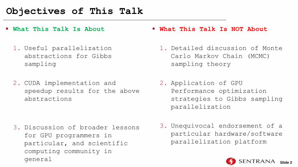
Objectives of This Talk
What This Talk Is About
1. Useful parallelization
abstractions for Gibbs
sampling
2. CUDA implementation and
speedup results for the above
abstractions
3. Discussion of broader lessons
for GPU programmers in
particular, and scientific
computing community in
general
What This Talk Is NOT About
1. Detailed discussion of Monte
Carlo Markov Chain (MCMC)
sampling theory
2. Application of GPU
Performance optimization
strategies to Gibbs sampling
parallelization
3. Unequivocal endorsement of a
particular hardware/software
parallelization platform
Slide 3
1. My Background
2. Why HB modeling in QM?
3. Introduction to Gibbs Sampling
4. Introduction to Univariate Slice Sampler
5. Single-chain Parallelization Strategies for Gibbs Sampling
6. Taxonomy of Variable Blocks
7. GPU Parallelization of Block Parallel, Log-Posterior Serial Variables
8. GPU Parallelization of Block Serial, Log-Posterior Parallel Variables
9. GPU Parallelization of Block Parallel, Log-Posterior Parallel
Variables
10. Speedup Results and Cost-Benefit Analysis (comparison of Serial
C/OpenMP/MPI/CUDA/VML)
11. Lessons Learned
Table of Contents
Slide 4
Background
Academic/programming background:
― Ph.D. in Physics / Computational Neuroscience
― Used MATLAB for thesis
― Entered programming world 3 years ago, starting with C#
― Gradually transitioned to C++ and C
― First serious exposure to GPU programming at GTC 2010
― Began CUDA programming in March 2011
My work:
― Our company (Sentrana) builds quantitative marketing software, with a
focus on Foodservice industry
― Our headcount is ~50, with ~25 business application software
developers, 3 full-time modelers
― Scientific computing is transitioning from a one-man show to a
separate department
Slide 5
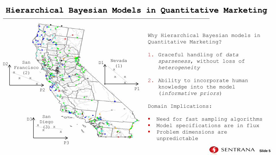
Hierarchical Bayesian Models in Quantitative Marketing
x
x
x
x
P1
D1 Nevada
(1)
x
x
x
x
P2
D2 San
Francisco
(2)
x
x x
x
San
Diego
(3)
P3
D3
Why Hierarchical Bayesian models in
Quantitative Marketing?
1. Graceful handling of data
sparseness, without loss of
heterogeneity
2. Ability to incorporate human
knowledge into the model
(informative priors)
Domain Implications:
Need for fast sampling algorithms
Model specifications are in flux
Problem dimensions are
unpredictable
Slide 6
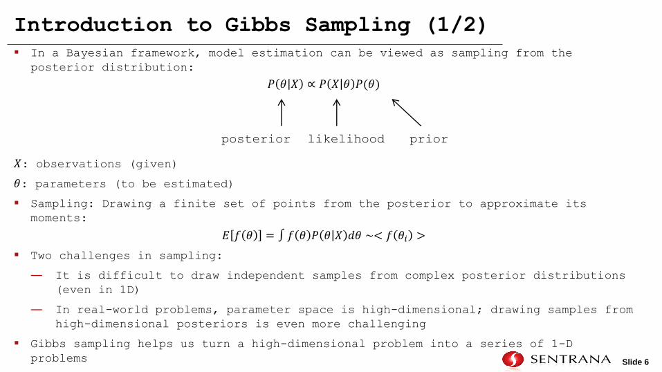
In a Bayesian framework, model estimation can be viewed as sampling from the
posterior distribution:
𝑃 𝜃 𝑋 ∝ 𝑃 𝑋 𝜃 𝑃(𝜃)
𝑋: observations (given)
𝜃: parameters (to be estimated)
Sampling: Drawing a finite set of points from the posterior to approximate its
moments:
𝐸 𝑓 𝜃 = ∫ 𝑓 𝜃 𝑃 𝜃 𝑋 𝑑𝜃 ∼< 𝑓 𝜃𝑖 >
Two challenges in sampling:
― It is difficult to draw independent samples from complex posterior distributions
(even in 1D)
― In real-world problems, parameter space is high-dimensional; drawing samples from
high-dimensional posteriors is even more challenging
Gibbs sampling helps us turn a high-dimensional problem into a series of 1-D
problems
Introduction to Gibbs Sampling (1/2)
posterior likelihood prior
Slide 7
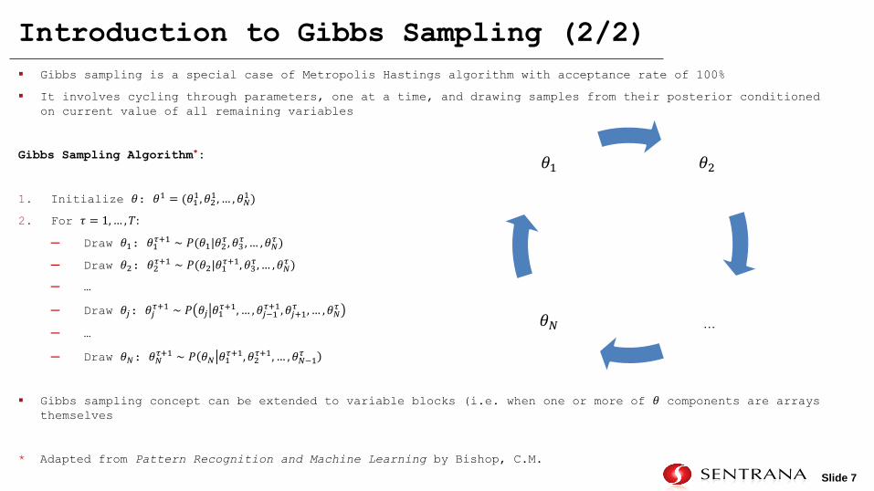
Gibbs sampling is a special case of Metropolis Hastings algorithm with acceptance rate of 100%
It involves cycling through parameters, one at a time, and drawing samples from their posterior conditioned
on current value of all remaining variables
Gibbs Sampling Algorithm*:
1. Initialize 𝜃: 𝜃1 = (𝜃11, 𝜃21, … , 𝜃𝑁
1)
2. For 𝜏 = 1,… , 𝑇:
─ Draw 𝜃1: 𝜃1𝜏+1 ∼ 𝑃(𝜃1|𝜃2
𝜏, 𝜃3𝜏, … , 𝜃𝑁
𝜏 )
─ Draw 𝜃2: 𝜃2𝜏+1 ∼ 𝑃(𝜃2|𝜃1
𝜏+1, 𝜃3𝜏, … , 𝜃𝑁
𝜏 )
─ …
─ Draw 𝜃𝑗: 𝜃𝑗𝜏+1 ∼ 𝑃 𝜃𝑗 𝜃1
𝜏+1, … , 𝜃𝑗−1𝜏+1, 𝜃𝑗+1
𝜏 , … , 𝜃𝑁𝜏
─ …
─ Draw 𝜃𝑁: 𝜃𝑁𝜏+1 ∼ 𝑃 𝜃𝑁 𝜃1
𝜏+1, 𝜃2𝜏+1, … , 𝜃𝑁−1
𝜏
Gibbs sampling concept can be extended to variable blocks (i.e. when one or more of 𝜃 components are arrays themselves
* Adapted from Pattern Recognition and Machine Learning by Bishop, C.M.
Introduction to Gibbs Sampling (2/2)
𝜃2
… 𝜃𝑁
𝜃1
Slide 8
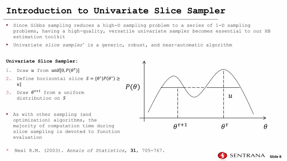
Since Gibbs sampling reduces a high-D sampling problem to a series of 1-D sampling
problems, having a high-quality, versatile univariate sampler becomes essential to our HB
estimation toolkit
Univariate slice sampler* is a generic, robust, and near-automatic algorithm
Univariate Slice Sampler:
* Neal R.M. (2003). Annals of Statistics, 31, 705-767.
Introduction to Univariate Slice Sampler
𝜃𝜏 𝜃
𝑃(𝜃) 𝑢
𝜃𝜏+1
1. Draw 𝑢 from unif[0, 𝑃(𝜃𝜏)]
2. Define horizontal slice 𝑆 = {𝜃∗|𝑃 𝜃∗ ≥𝑢}
3. Draw 𝜃𝜏+1 from a uniform distribution on 𝑆
As with other sampling (and
optimization) algorithms, the
majority of computation time during
slice sampling is devoted to function
evaluation
Slide 9
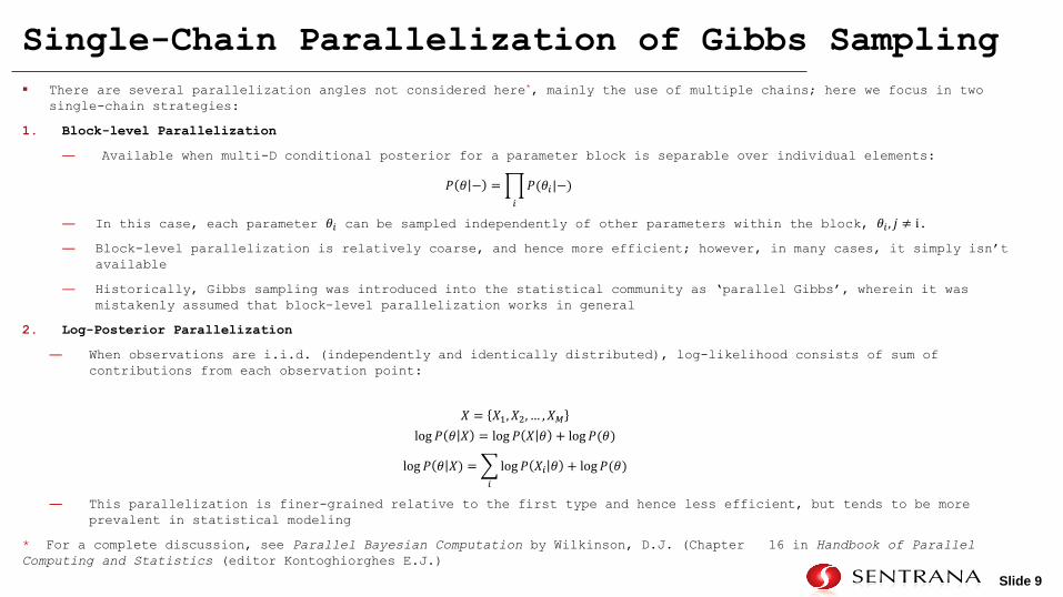
There are several parallelization angles not considered here*, mainly the use of multiple chains; here we focus in two
single-chain strategies:
1. Block-level Parallelization
― Available when multi-D conditional posterior for a parameter block is separable over individual elements:
𝑃 𝜃 − = 𝑃(𝜃𝑖|−)
𝑖
― In this case, each parameter 𝜃𝑖 can be sampled independently of other parameters within the block, 𝜃𝑖 , 𝑗 ≠ i.
― Block-level parallelization is relatively coarse, and hence more efficient; however, in many cases, it simply isn’t
available
― Historically, Gibbs sampling was introduced into the statistical community as ‘parallel Gibbs’, wherein it was
mistakenly assumed that block-level parallelization works in general
2. Log-Posterior Parallelization
― When observations are i.i.d. (independently and identically distributed), log-likelihood consists of sum of
contributions from each observation point:
𝑋 = 𝑋1, 𝑋2, … , 𝑋𝑀
log 𝑃 𝜃 𝑋 = log 𝑃 𝑋 𝜃 + log 𝑃(𝜃)
log 𝑃 𝜃 𝑋) = log 𝑃 𝑋𝑖 𝜃 + log 𝑃(𝜃)
𝑖
― This parallelization is finer-grained relative to the first type and hence less efficient, but tends to be more
prevalent in statistical modeling
* For a complete discussion, see Parallel Bayesian Computation by Wilkinson, D.J. (Chapter 16 in Handbook of Parallel
Computing and Statistics (editor Kontoghiorghes E.J.)
Single-Chain Parallelization of Gibbs Sampling

Slide 10
All permutations of block-level and log-posterior parallelization are
possible, leading to four types of parameter blocks:
1. Block-serial, log-posterior-serial (BS-LPS) No parallelization
opportunity
2. Block-parallel, log-posterior-serial (BP-LPS) Single-faceted, easy to
implement, high modular speedup, low overall impact
3. Block-serial, log-posterior-parallel (BS-LPP) Single-faceted, modestly
difficult to implement, modest modular speedup, good overall impact
4. Block-parallel, log-posterior-parallel (BP-LPP) dual-faceted, difficult
to implement, high modular speedup, high overall impact
Organization of GPU into blocks and threads naturally maps to dual-faceted
parallelization for BP-LPP parameter blocks
However, taking full advantage of the available silicon on the GPU requires
significant code reorganization
Taxonomy of Parameter Blocks
Slide 11
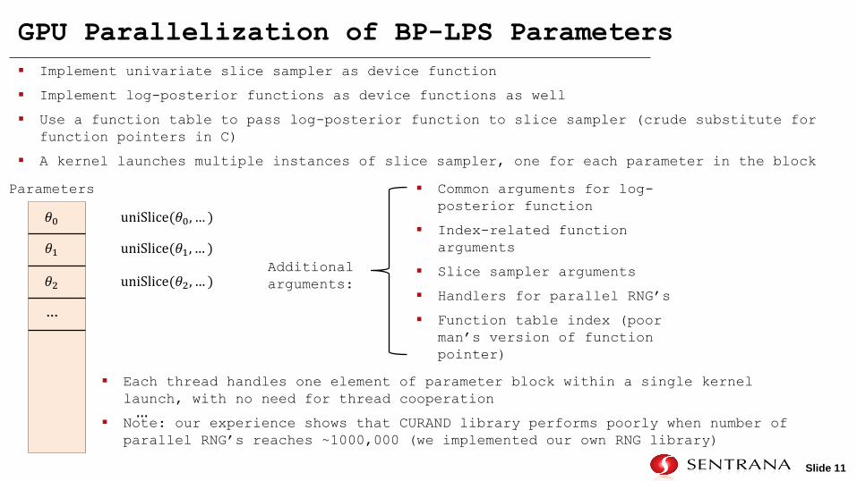
Implement univariate slice sampler as device function
Implement log-posterior functions as device functions as well
Use a function table to pass log-posterior function to slice sampler (crude substitute for
function pointers in C)
A kernel launches multiple instances of slice sampler, one for each parameter in the block
GPU Parallelization of BP-LPS Parameters
𝜃0
𝜃1
𝜃2
…
uniSlice(𝜃0, … )
uniSlice(𝜃1, … )
uniSlice(𝜃2, … )
…
Additional
arguments:
Common arguments for log-
posterior function
Index-related function
arguments
Slice sampler arguments
Handlers for parallel RNG’s
Function table index (poor
man’s version of function
pointer)
Each thread handles one element of parameter block within a single kernel
launch, with no need for thread cooperation
Note: our experience shows that CURAND library performs poorly when number of
parallel RNG’s reaches ~1000,000 (we implemented our own RNG library)
Parameters

Slide 12
Sampling of elements within the block must happen serially
Parallelization occurs while evaluating log-posterior function for a single element (due
to i.i.d. nature of observed data)
We employ a two-stage scatter-gather approach for GPU parallelization
GPU Parallelization of BS-LPP Parameters
𝑋[0]
𝑋[1]
𝑋[2]
…
log 𝑃 𝑋 0 𝜃)
log𝑃(𝑋[1]|𝜃)
log𝑃(𝑋[2]|𝜃)
…
Observations
Step 1: Scatter + Partial Gather
(executed on device)
Step 2: Final Gather
(some or all executed on host)
𝑆0 = log𝑃(𝑋[𝑖]|𝜃)
3
𝑖=1
𝑆1 = log𝑃(𝑋[𝑖]|𝜃)
6
𝑖=4
…
log 𝑃 𝜃 𝑋 = 𝑆𝑘𝑘
+ log𝑃(𝜃)

Slide 13
We can parallelize at block level as well as log-posterior level
CUDA implementation is more involved than first two cases
Step 1: Create a vectorized version of slice sampler
Vectorized slice sampler takes advantage of a parallel function evaluator (FuncPar), with
each of n elements corresponding to one conditionally-independent parameter in the block
Since each parameter may need a different number of iterations before acceptance, we can
keep track by using selectVec and use parallel hardware more efficiently
GPU Parallelization of BP-LPP Parameters (1/4) –
Vectorization of Slice Sampler
Standard Slice Sampler Vectorized Slice Sampler
typedef double (*Func)(
double x
, const void *args
);
double uniSlice(
Func f
, double x0
, const void *args
, SliceArg &sliceArgs
);
typedef void (*FuncPar)(
int n,
const double *xVec
, const void **argsVec
, const bool *selectVec
, double *fVec
);
void uniSlicePar(
FuncPar f
, int n
, const double *x0Vec
, const void **argsVec
, SliceArg &sliceArgs
, double *xVec
);
Slide 14
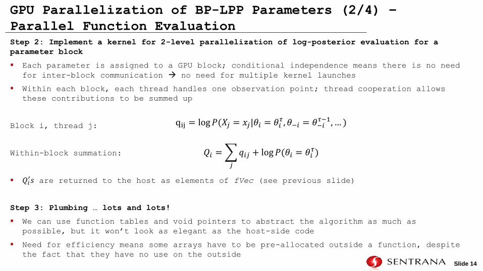
Step 2: Implement a kernel for 2-level parallelization of log-posterior evaluation for a
parameter block
Each parameter is assigned to a GPU block; conditional independence means there is no need
for inter-block communication no need for multiple kernel launches
Within each block, each thread handles one observation point; thread cooperation allows
these contributions to be summed up
Block i, thread j:
Within-block summation:
𝑄𝑖′𝑠 are returned to the host as elements of fVec (see previous slide)
Step 3: Plumbing … lots and lots!
We can use function tables and void pointers to abstract the algorithm as much as
possible, but it won’t look as elegant as the host-side code
Need for efficiency means some arrays have to be pre-allocated outside a function, despite
the fact that they have no use on the outside
GPU Parallelization of BP-LPP Parameters (2/4) –
Parallel Function Evaluation
qij = log𝑃(𝑋𝑗 = 𝑥𝑗|𝜃𝑖 = 𝜃𝑖𝜏, 𝜃−𝑖 = 𝜃−𝑖
𝜏−1, … )
𝑄𝑖 = 𝑞𝑖𝑗 + log𝑃(𝜃𝑖 = 𝜃𝑖𝜏)
𝑗
Slide 15
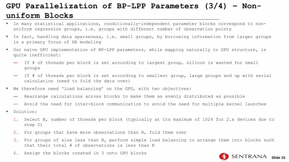
In many statistical applications, conditionally-independent parameter blocks correspond to non-
uniform regression groups, i.e. groups with different number of observation points
In fact, handling data sparseness, i.e. small groups, by borrowing information from larger groups
is a primary focus of HB modeling
Our naïve GPU implementation of BP-LPP parameters, while mapping naturally to GPU structure, is
quite inefficient:
― If # of threads per block is set according to largest group, silicon is wasted for small
groups
― If # of threads per block is set according to smallest group, large groups end up with serial
calculation (need to fold the data over)
We therefore need ‘load balancing’ on the GPU, with two objectives:
― Rearrange calculations across blocks to make them as evenly distributed as possible
― Avoid the need for inter-block communication to avoid the need for multiple kernel launches
Solution:
1. Select N, number of threads per block (typically at its maximum of 1024 for 2.x devices due to
step 2)
2. For groups that have more observations than N, fold them over
3. For groups of size less than N, perform simple load balancing to arrange them into blocks such
that their total # of observations is less than N
4. Assign the blocks created in 3 onto GPU blocks
GPU Parallelization of BP-LPP Parameters (3/4) – Non-
uniform Blocks
Slide 16
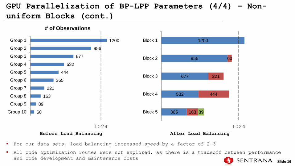
GPU Parallelization of BP-LPP Parameters (4/4) – Non-
uniform Blocks (cont.)
60
89
163
221
365
444
532
677
956
1200
Group 10
Group 9
Group 8
Group 7
Group 6
Group 5
Group 4
Group 3
Group 2
Group 1
# of Observations
1024
Before Load Balancing After Load Balancing
365
532
677
956
1200
163
444
221
60
89 Block 5
Block 4
Block 3
Block 2
Block 1
1024
For our data sets, load balancing increased speed by a factor of 2-3
All code optimization routes were not explored, as there is a tradeoff between performance
and code development and maintenance costs

Slide 17
Speedup Results
Parameter Block Problem Spec Serial-CPU OpenMP
(8 cores)
CUDA
BP-LPS (block parallelization) Block size: ~4 million
CPU execution time for parallelized task:
~7sec 1.0x ~3x ~100x
BS-LPP (log-posterior
parallelization)
Number of observations: 6390
CPU execution time for parallelized task:
~7msec 1.0x ~5x ~23x
BP-LPP (dual parallelization) Number of groups: 500
Number of observations per group: 500
CPU execution time for parallelized task:
~2sec
1.0x ~6x ~100x
Details:
― CPU: Intel Xeon W3680, 3.33GHz; 12 cores; 2GB/core RAM (8 cores used for OpenMP since more than 8
reduced performance); code compiled with –O2 flag
― GPU: GeForce GTX 580 (all GPU code was double-precision; fast math option turned on)
― Measurements include: per sampling (recurring) data transfer between host and device
― Measurements exclude: initial (one-time) data transfer between host and device
Other tests:
― BP-LPP MPI-parallelization was tested on a commercial cluster; we saw speedups of ~50-60x relative to
single-threaded code (on same cluster), saturating at ~16 nodes / 128 cores

Slide 18
Total Model Cost = Development Cost + Execution Cost
Development cost
― Time and expertise needed to specify HB model (hierarchy definition, variable selection / transformation, etc)
iterative, requires building, running, and inspecting early versions
― Time and expertise needed to convert high-level, low-performance code (e.g. in R) to low-level, high-performance code
(C/C++/CUDA); includes debugging/testing
― Code maintenance
Execution cost
― Wall-time needed to estimate model coefficients (i.e. run Gibbs sampling)
― Total core-hours
How does CUDA stack up against alternatives on these two metrics?
― Development cost
• By reducing execution time, it allows modelers to iterate on models faster trial-and-error (to some degree)
replaces mathematical expertise
• However, it shifts the burden from mathematical and statistical expertise to programming time and expertise (C is
harder than R; CUDA is harder than C)
― Execution cost
• Not only does it reduce wall-time, but it also is cheaper (our calculations showed that porting our code from CPU to
GPU leads to savings of ~5-10x)
• On the other hand, maintaining in-house GPU servers adds to required skill set for system administrators
• In comparison to MPI and Intel’s Vector Math Library, CUDA requires about as much code modification (if not less)
and the return on investment is higher
Total Cost Analysis
Slide 19
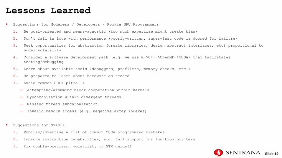
Suggestions for Modelers / Developers / Rookie GPU Programmers
1. Be goal-oriented and means-agnostic (too much expertise might create bias)
2. Don’t fall in love with performance (poorly-written, super-fast code is doomed for failure)
3. Seek opportunities for abstraction (create libraries, design abstract interfaces, etc) proportional to
model volatility
4. Consider a software development path (e.g. we use R->C++->OpenMP->CUDA) that facilitates
testing/debugging
5. Learn about available tools (debuggers, profilers, memory checks, etc.)
6. Be prepared to learn about hardware as needed
7. Avoid common CUDA pitfalls
─ Attempting/assuming block cooperation within kernels
─ Synchronization within divergent threads
─ Missing thread synchronization
─ Invalid memory access (e.g. negative array indexes)
Suggestions for Nvidia
1. Publish/advertise a list of common CUDA programming mistakes
2. Improve abstraction capabilities, e.g. full support for function pointers
3. Fix double-precision volatility of GTX cards!!
Lessons Learned