Embed Size (px)
Citation preview
Gradient and Hamiltonian Dynamics� SomeApplications to Neural Network Analysis and
System Identi�cation
by
James Walter Howse IV
B�S� Physics� Lehigh University� ����
M�S� Electrical Engineering� University of Central Florida� ����
DISSERTATION
Submitted in Partial Ful�llment of the
Requirements for the Degree of
Doctor of Philosophy in Engineering
The University of New Mexico
Albuquerque� New Mexico
December� ����

c������ James Walter Howse IV
iii

To my parents �
who gave me a thirst for knowledge
and the drive to seek it out�
To my wife �
who was a constant source of
both inspiration and support�
iv

Acknowledgements
I would like to thank a number of people from both my academic and personal worlds for theirhelp over the years� First and foremost I would like to thank my wife Sarah for her tremendousemotional and �nancial support during my dissertation� Without her generous and constantassistance this manuscript would never have been completed� I would like to thank HarryRobb� Bill Wood� and Dan Thornton for helping me to realize and create the person that Iam today� you three have made my world far brighter� On the technical side� I would like tothank my advisors Chaouki Abdallah and Greg Heileman for their patience in allowing me topursue my Ph�D� in my own way� even when it was against their better judgment� I feel thatin the long run I bene�ted greatly from this freedom� and I hope that they did as well� Also Iwould like to thank Greg for convincing me to come to UNM in the �rst place and for doinghis best to get me set up here� Thanks go to Chaouki for stimulating my interest in controland systems theory� and for guiding me through these complex topics� Vangelis Coutsias hasanswered all of my numerous mathematics questions and taught me most of the dynamics thatI currently know� Tom Caudell has always made me think about how to better ground myresearch� and has also given me some very good advice� Don Hush has been an inspiration forme by allowing himself to be a sounding board for a stream of my �great ideas� I really valuehis insightful comments� I would also like to thank Bob Cromp for telling me �You cant builda reputation based on what you intend to do� Lastly I would like to thank both D�T� Suzukiand the members of � whose words I have spent many pleasant hours pondering�
Contained in everything I doTheres a love� I feel for youProclaimed in everything I writeYoure the light� burning brightlyOnward through the night� of my life
Onward by Chris Squire
And I gave my heart to know wisdom� and to know madness and folly�But I perceived that this merely torments the spirit�For in much wisdom there is much grief�And he that increaseth knowledge� increaseth sorrow�
Ecclesiastes ���� ��
The Way that can be told of is not the eternal Way�The name that can be named is not the eternal name�The Nameless is the origin of Heaven and Earth�The Named is the mother of all things�Therefore let there always be non�being so we may see their subtlety�And let there always be being so we may see there outcome�The two are the same�But after they are produced� they have di�erent names�
The Tao�te Ching verse �
v
Gradient and Hamiltonian Dynamics� SomeApplications to Neural Network Analysis and
System Identi�cation
by
James Walter Howse IV
ABSTRACT OF DISSERTATION
Submitted in Partial Ful�llment of the
Requirements for the Degree of
Doctor of Philosophy in Engineering
The University of New Mexico
Albuquerque� New Mexico
December� ����
Gradient and Hamiltonian Dynamics� SomeApplications to Neural Network Analysis and
System Identi�cation
by
James Walter Howse IV
B�S� Physics� Lehigh University� ����
M�S� Electrical Engineering� University of Central Florida� ����
Ph�D� Electrical Engineering� University of New Mexico� ����
Abstract
The work in this dissertation is based on decomposing system dynamics into the sum of dissi�
pative �e�g� convergent� and conservative �e�g� periodic� components� Intuitively� this can be
viewed as decomposing the dynamics into a component normal to some surface and components
tangent to other surfaces� First� this decomposition was applied to existing neural network ar�
chitectures to analyze their dynamic behavior� Second� this formalism was employed to create
models which learn to emulate the behavior of actual systems� The premise of this approach
is that the process of system identi�cation can be considered in two stages� model selection
and parameter estimation� In this dissertation a technique is presented for constructing dy�
namical systems with desired qualitative properties� Thus� the model selection stage consists
of choosing the dissipative and conservative portions appropriately so that a certain behavior
is obtainable� By choosing the parametrization of the models properly� a learning algorithm
has been devised and proven to always converges to a set of parameters for which the error
between the output of the actual system and the model vanishes� So these models and the
associated learning algorithm are guaranteed to solve certain types of nonlinear identi�cation
problems�
vii
Contents
� Introduction �
� Mathematical Formalism �
��� Review of Ordinary Di�erential Equations � � � � � � � � � � � � � � � � � � � � � �
����� Terms from Topology � � � � � � � � � � � � � � � � � � � � � � � � � � � � �
����� De�nition of the Phase Space � � � � � � � � � � � � � � � � � � � � � � � � ��
����� Existence and Uniqueness of Solutions � � � � � � � � � � � � � � � � � � � ��
����� Equilibrium Solutions � � � � � � � � � � � � � � � � � � � � � � � � � � � � ��
����� Recurrent Solutions � � � � � � � � � � � � � � � � � � � � � � � � � � � � � ��
����� Integral Manifolds � � � � � � � � � � � � � � � � � � � � � � � � � � � � � � ��
����� Stability of Solutions � � � � � � � � � � � � � � � � � � � � � � � � � � � � � ��
����� Asymptotic Behavior of Solutions � � � � � � � � � � � � � � � � � � � � � � ��
����� Lyapunov Stability � � � � � � � � � � � � � � � � � � � � � � � � � � � � � � ��
������ Structural Stability � � � � � � � � � � � � � � � � � � � � � � � � � � � � � � ��
��� Properties of Gradient Systems � � � � � � � � � � � � � � � � � � � � � � � � � � � ��
��� Properties of Gradient�Like Systems � � � � � � � � � � � � � � � � � � � � � � � � ��
��� Properties of Hamiltonian Systems � � � � � � � � � � � � � � � � � � � � � � � � � ��
��� Properties of Hamiltonian�Like Systems � � � � � � � � � � � � � � � � � � � � � � ��
� Gradient�Hamiltonian Analysis ��
viii
Contents
��� Review of Lyapunov Function Results � � � � � � � � � � � � � � � � � � � � � � � ��
��� Gradient�Like Formulation of the Constant Weight Case � � � � � � � � � � � � � ��
����� Application to an Additive Network � � � � � � � � � � � � � � � � � � � � ��
����� Application to a Multiplicative Network � � � � � � � � � � � � � � � � � � ��
����� A Control Theory Viewpoint � � � � � � � � � � � � � � � � � � � � � � � � ��
��� Gradient�Like Formulation of the Updated Weight Case � � � � � � � � � � � � � ��
����� Application to Multilayer Networks � � � � � � � � � � � � � � � � � � � � � ��
����� Application to Symmetric Hebbian Learning � � � � � � � � � � � � � � � ��
����� Application to Anti�Hebbian Learning � � � � � � � � � � � � � � � � � � � ��
����� Application to Di�erential Hebbian Learning � � � � � � � � � � � � � � � ��
����� Application to Higher�Order Networks � � � � � � � � � � � � � � � � � � � ��
��� Simulation of a Simple Gradient�like Network � � � � � � � � � � � � � � � � � � � ��
��� Review of Gradient�Hamiltonian Decomposition Results � � � � � � � � � � � � � ��
��� Gradient�Hamiltonian Formulation of the Updated Weight Case � � � � � � � � � ��
����� Application to Asymmetric Hebbian Learning � � � � � � � � � � � � � � � ��
����� Application to Gated Learning � � � � � � � � � � � � � � � � � � � � � � � ��
����� Application to Feedforward Networks � � � � � � � � � � � � � � � � � � � ��
��� Existing Recurrent Networks as Gradient�Hamiltonian Systems � � � � � � � � � ��
��� Assessment of the Gradient�Hamiltonian Decomposition for Analysis � � � � � � ��
� Gradient�Hamiltonian Synthesis ��
��� Review of Cohens Model � � � � � � � � � � � � � � � � � � � � � � � � � � � � � � ��
��� Learning the Parameters in Cohens Model � � � � � � � � � � � � � � � � � � � � ��
��� Simulation of the Proposed Learning Algorithm � � � � � � � � � � � � � � � � � � ��
��� Assessment of the Gradient�Hamiltonian Model for System Identi�cation � � � � ��
ix
Contents
� Conclusion ��
��� Future Research � � � � � � � � � � � � � � � � � � � � � � � � � � � � � � � � � � � ���
A Basic Topology ��
B Proofs for Chapter � ��
Bibliography ���
x
List of Figures
��� Comparison between vector and direction �elds� Example ��� � � � � � � � � � � ��
��� The construction of a Poincar�e map for a closed orbit � � � � � � � � � � � � � � ��
��� The phase spaces of three di�erent oscillators� Example ��� � � � � � � � � � � � ��
��� Trajectories in phase space� Example ��� � � � � � � � � � � � � � � � � � � � � � � ��
��� Comparison of gradient and gradient�like systems � � � � � � � � � � � � � � � � � ��
��� Comparison of Hamiltonian and Hamiltonian�like systems � � � � � � � � � � � � ��
��� Control theory diagram of a multiplicative system � � � � � � � � � � � � � � � � ��
��� Con�guration of example network� Section ��� � � � � � � � � � � � � � � � � � � � ��
��� Time evolution of the state variables� Section ��� � � � � � � � � � � � � � � � � � ��
��� Three dimensional cross�section of the phase space � � � � � � � � � � � � � � � � ��
��� Two dimensional cross�section of the phase space � � � � � � � � � � � � � � � � � ��
��� Time evolution of the gradient potential � � � � � � � � � � � � � � � � � � � � � � ��
��� Cross�sections of the gradient potential � � � � � � � � � � � � � � � � � � � � � � � ��
��� Con�guration of oscillating network� Example ��� � � � � � � � � � � � � � � � � � ��
��� Plot of a function which approximates max��� �x � ����� � � � � � � � � � � � � � ��
���� Time evolution of the states� Example ��� � � � � � � � � � � � � � � � � � � � � � ��
���� Gradient and Hamiltonian vector �elds� Example ��� � � � � � � � � � � � � � � � ��
���� Total vector �eld and example trajectories� Example ��� � � � � � � � � � � � � � ��
���� Graph of gradient potential� Example ��� � � � � � � � � � � � � � � � � � � � � � ��
xi
List of Figures
���� Gradient and Hamiltonian vector �elds� Example ��� � � � � � � � � � � � � � � � ��
���� Example trajectories for two di�erent Hamiltonians� Example ��� � � � � � � � � ��
���� Alternate gradient and Hamiltonian vector �elds� Example ��� � � � � � � � � � ��
��� Scheme for construction of a potential function � � � � � � � � � � � � � � � � � � ��
��� Vector �eld and time evolution of the states� Example ��� � � � � � � � � � � � � ��
��� Vector �eld and time evolution of the states� Example ��� � � � � � � � � � � � � ��
��� Partitioning a vector �eld with level surfaces � � � � � � � � � � � � � � � � � � � ��
��� Vector �eld and time evolution of the states� Example ��� � � � � � � � � � � � � ��
��� Construction of a single period attractor � � � � � � � � � � � � � � � � � � � � � � ��
��� Graph of an example potential function � � � � � � � � � � � � � � � � � � � � � � ��
��� The ��norm of the gradient krxV�x�k � � � � � � � � � � � � � � � � � � � � � � � ��
��� Time evolution of the state and parameter errors � � � � � � � � � � � � � � � � � ��
���� Magnitude of the power spectral density versus frequency � � � � � � � � � � � � ��
���� Phase plot when trained with one input and tested with another � � � � � � � � ��
xii
List of Tables
��� Equilibrium solutions for I� � �� � � � � � � � � � � � � � � � � � � � � � � � � � � ��
��� Equilibrium solutions for I� � ��� � � � � � � � � � � � � � � � � � � � � � � � � � ��
��� Eigenvalues of the Jacobian � � � � � � � � � � � � � � � � � � � � � � � � � � � � � ��
��� Eigenvalues of the Hessian and potential value � � � � � � � � � � � � � � � � � � ��
��� Comparison of actual and estimated parameter values � � � � � � � � � � � � � � ��
��� Comparison between target and test trajectories � � � � � � � � � � � � � � � � � ��
xiii
Glossary
vy The transpose of the n�element vector v � �v�� v�� � � � � vn��
�v The total time derivativedv
dtof the vector v�
jsj The absolute value of the scalar s�
s� � s� The scalar s� is much greater than the scalar s��
kvk The norm of the vector v� de�ned as kvk � �jv�jp� jv�jp� � � �� jvnjp��
p
for some p such that � � p ���
vyw The inner product of the two n�element vectors v and w� de�ned as
vyw �Pn
i�� vi wi�
DE�v�w� The Euclidean distance between the vectors v and w� de�ned as
DE�v�w� � kv �wk�
f � S� � S� f is a function which maps members of the set S� to members of the
set S��
v � S v is a member of the set S�
S� S� The set S� is a subset of the set S�� meaning that S� may contain all
members of S��
S� S� The set S� is a proper subset of the set S�� meaning that S� may not
contain all members of S��
S� � S� Take the union of the sets S� and S�� meaning collect all elements
occuring in either set�
S� � S� Take the intersection of the sets S� and S�� meaning collect all elements
occuring in both sets�
xiv
Glossary
S� n S� Subtract the members of set S� from set S�� meaning remove any
elements from S� which occur in S��
S� S� Take the Cartesian product of the sets S� and S��
� The empty set�
� for all
R the real numbers
N the natural numbers� �� �� �� � � �
rvF�v� The gradient of the scalar function F�v�� de�ned as the vector rvF�v�
�
��F
�v�
�F
�v�� � � �F
�vn
�y�
�F�v� The total time derivativedF
dtof the scalar function F�v�� given by
�F�v� � rvF�v�y �v�
Tr�M � Sum the diagonal elements of the matrixM � Tr�M � �Pn
i��mii� This
quantity is called the trace�
Diag�m��m�� � � � �mn� Construct a matrix with the elements m�� m�� � � � � mn along the
diagonal and wherein all other elements are ��
M �N Take the product of each element of the matrix M with the corre�
sponding element of the matrixN � �M �N �ij � mij nij� This operator
is called the Schur product�
ODE Ordinary Di�erential Equation
xv
Chapter �
Introduction
Mathematical systems theory is concerned with the process of �nding mathematically well�
structured models which adequately describe real systems� One of the great challenges remain�
ing in this �eld is understanding the use of nonlinear systems in modeling physical phenomena�
While it is true that many physical systems can be modeled by a linear system if the operating
conditions are su�ciently restricted� this approach often leads to a model whose operating
range is far too small to be practically useful� In order to remove this limitation� one typically
must use a nonlinear system when modeling real systems� Three extremely useful properties
of linear systems� all discussed in Kailath ������� are their stability properties� their natural
parametrization and the principle of superposition� Any continuous�time time�invariant linear
system can be written in the form
�x � Ax�Bu�
y � C x������
where x � Rn is the state vector� u � R
m is the input vector� and y � Rp is the output
vector� Furthermore� A � Rn�n � B � R
n�m � and C � Rp�n are matrices of real constants�
The elements of these matrices are the natural parametrization of the linear system in the
sense that criteria such as stability� controllability and observability can be de�ned in terms of
these quantities alone� For time�variant systems the elements of these matrices become explicit
functions of time� The linear system in Equation ����� is either globally exponentially stable
or unstable depending on the eigenvalues of the matrix A� So the states either converge to or
diverge from the equilibrium point x � at an exponential rate� The principle of superposition
states that for a linear system the output response to a linear combination of inputs is identical
to a linear combination of the output responses to the individual inputs� This means that the
system output can be decomposed into a sum of output �modes� each of which depends on
one and only one input �mode� This decomposition is the basis of many powerful analysis
Chapter �� Introduction �
and synthesis methods for linear systems�
None of these properties are possessed by general nonlinear systems� This is because no
generic description containing all nonlinear systems is known� Such a description would be
analogous to Equation ������ Since the class of nonlinear systems consists by de�nition of all
systems which are not linear� it seems unlikely that such a universal form even exists� One
very general� if not universal� form for nonlinear systems is
�x � f�x�u��
y � h�x�������
where x� u � and y have the same meaning as those vectors described in Equation ������
Additionally� f � Rn Rm � R
n is the state�input to state mapping and h � Rn � Rp is the
state to output mapping� Surprisingly� it was shown by Sontag ������ that there is no loss of
generality by limiting the output function to be linear �i�e� y � C x�� One class of nonlinear
models which has received a great deal of attention are neural networks� A class of neural
networks are de�ned in Sontag ������ as systems of the form
��x � �� �A �x� �B u�� ����a�
y � �C �x� ����b�
where �x � R�n is the state vector� u � Rm is the input vector� and y � Rp is the output vector�
Furthermore� �A � R�n��n� �B � R
�n�m� and �C � Rp��n are matrices of real constants and
� � R�n � R�n is a nonlinear function� Neural networks of this form are shown in Sontag ������
to be capable of approximating any nonlinear dynamical system over a compact subset of the
state space �i�e� a compact subset of R�n� and a �nite time interval� Note that this result requires
that the function � satisfy a few technical conditions� A similar result is obtained in Funahashi
and Nakamura ������ for neural networks of a slightly di�erent form� The relationship between
these two results is discussed in �Zbikowski ������� Note that neither of these results guarantees
an e�cient model� meaning that it is possible that �n� n�
There are two di�culties associated with using the systems in Equation ����� for modeling�
The �rst di�culty is the fact that this model can not be decomposed into components whose
behavior is indicative of the behavior of the whole system� Since there is no notion of super�
position� it tends to be di�cult to analyze the behavior of neural networks� or to synthesize
neural networks which have a speci�c qualitative behavior� The second di�culty is related to
�nding the parameters values in �A � �B � and �C which cause the model to emulate the behavior
of some real system� However� before discussing this di�culty some background concepts need
to be reviewed� In order to use the system in Equation ����� as a model for a real system� the
behavior of the model must be �tted to the behavior of the real system� This �tting can be
Chapter �� Introduction �
done using one of two conceptual frameworks� The �rst framework requires that all elements
of the state vector x be measurable at all times� In this case the feedback structure de�ned by
Equation ����a� can be unfolded into a feedforward structure which contains one layer for every
instant in time� This is tractable because when gathering data to �t the models behavior to
the real system� the real system can only be observed for a �nite time and measured a �nite
number of times� The �tting is then done by �nding the parameter values which minimize the
functional
E ��
�
Z tf
ti
� y���� y���p��y � y���� y���p�� d�� �����
where the vector y��� contains measurements of the output of the actual system� and y���p�
contains the output of the model for the parameter values in p� The graph of E with respect to
the model parameters p de�nes a surface with respect to the �nite�dimensional parameter space
called the error surface� Fitting the model to the actual system is then de�ned as searching
the space of all parameter values for those which occur at the minima of this surface� The
di�culty associated with the model in Equation ����� is that the parameters �A and �B enter
nonlinearly� This means that the surface de�ned by E is nonlinear� and in general will have
multiple minima�
There are two approaches to solving �nite�dimensional nonlinear optimization problems�
The trouble with all of these techniques is that they can not be guaranteed to converge to
�good estimates of the parameters in a �short period of time� The �rst approach is to move
�downhill on the surface E until that is no longer possible� at which point a minima of E has
been reached� This approach uses local information at each point on the surface to choose an
appropriate �downhill direction� Collectively� all of these methods belong to the family of local
optimization techniques� which are discussed at length in Luenberger ������� Note that two of
the most common training procedures for recurrent neural networks� backpropagation through
time� derived in Rumelhart� Hinton� and Williams ������� and real time recurrent learning�
derived in Robinson and Fallside ������� are based on this sort of optimization� Both of these
procedures were originally derived for discrete time systems� then re�derived for continuous time
systems heuristically in Pearlmutter ������� and rigorously using the calculus of variations in
Ramacher ������� The di�culty with all local nonlinear optimization techniques is that since
the error surface has multiple minima� there is no way of knowing which one will be found� In
fact� many such nonlinear optimization algorithms are not guaranteed to �nd any minima at
all�
The second approach to solving �nite�dimension nonlinear optimization problems is to try
to distinguish between the various local minima and to �nd the one for which the value of E is
the smallest� There are a variety of techniques for searching for the lowest point of the error
Chapter �� Introduction �
surface� many of which are outlined in Kan and Timmer ������� Very few of these methods
are used as learning algorithms for neural networks� One of the few exceptions is simulated
annealing� which is discussed as a learning algorithm in Ackley� Hinton� and Sejnowski �������
This technique is a member of the class of methods which seek a path on the error surface which
usually decreases the value of the error function� The general idea underlying such techniques
is that having used local descent to reach some point on the error surface� one jumps to a
randomly chosen point nearby� The local descent is always continued from this new point if
it has a lower value of E than the original point� and has some non�zero probability of being
continued from the new point even if it has a larger value of E than the original point� The
problem with all global nonlinear optimization techniques is that they are not guaranteed to
�nd the global minimum unless an in�nite amount of computation is performed� In practice
this means that such methods usually take an extremely long time to �nd a solution�
If the values of the state vector x can not be measured� then the recurrent network in
Equation ����a� can not be unfolded in time� This means that the parameters in the vector p in
Equation ����� can not be isolated� Hence the problem of �tting Equation ����� to data becomes
a search over the in�nite�dimensional space of all functions y���p�� rather than a search over
the �nite�dimensional space of all parameters p� In this case� the form of Equation ����� acts
to constrain the region of function space which should be searched� Optimization over in�nite�
dimensional spaces is also called functional optimization because E is the functional �i�e� a
function of functions� to be optimized� This sort of optimization is frequently done in optimal
control and is discussed in this context by Athans and Falb ������� The most common method
used to solve optimization problems of this type is dynamic programming� which was developed
by Bellman ������� The major problem with solving optimization problems of this type is that
only a very restricted class of these problems can be solved by dynamic programming�
In this dissertation a general description is attempted for a class of nonlinear systems
which can be decomposed into �modes� and whose parameters can be estimated using linear
optimization� The form that these systems take is
�x � P �x�rxV�x� �nXi��
Qi�x�rxV�x� �B g�u��
y � C x�
�����
First� the global stability of the system states depends only on some simple conditions on the
matrix P �x� and the function V�x�� Second� a simple condition on V�x� causes bounded in�
puts to result in ultimately bounded states� This means that if the �size of the input vector
u has some maximum value� then eventually the �size of the state vector x also has some
maximum value� Third� the matrices P �x�� Qi�x�� B� and C and the function V�x� form a
Chapter �� Introduction �
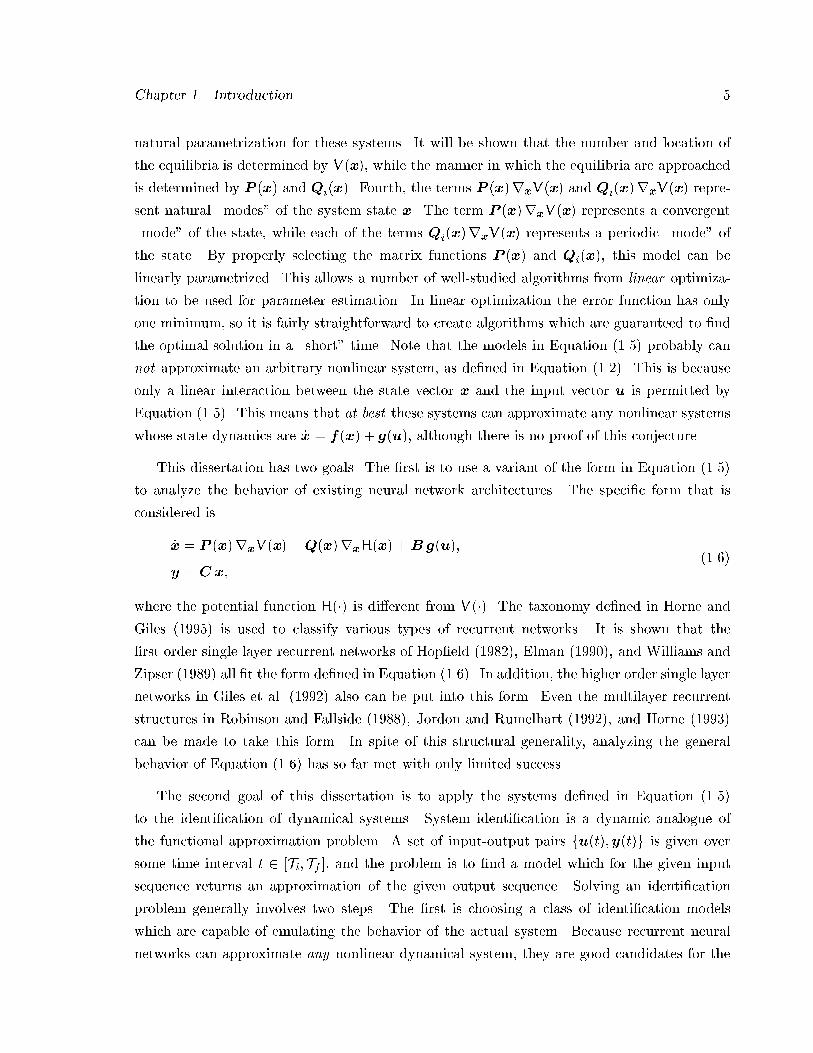
natural parametrization for these systems� It will be shown that the number and location of
the equilibria is determined by V�x�� while the manner in which the equilibria are approached
is determined by P �x� and Qi�x�� Fourth� the terms P �x�rxV�x� and Qi�x�rxV�x� repre�
sent natural �modes of the system state x� The term P �x�rxV�x� represents a convergent
�mode of the state� while each of the terms Qi�x�rxV�x� represents a periodic �mode of
the state� By properly selecting the matrix functions P �x� and Qi�x�� this model can be
linearly parametrized� This allows a number of well�studied algorithms from linear optimiza�
tion to be used for parameter estimation� In linear optimization the error function has only
one minimum� so it is fairly straightforward to create algorithms which are guaranteed to �nd
the optimal solution in a �short time� Note that the models in Equation ����� probably can
not approximate an arbitrary nonlinear system� as de�ned in Equation ������ This is because
only a linear interaction between the state vector x and the input vector u is permitted by
Equation ������ This means that at best these systems can approximate any nonlinear systems
whose state dynamics are �x � f�x� � g�u�� although there is no proof of this conjecture�
This dissertation has two goals� The �rst is to use a variant of the form in Equation �����
to analyze the behavior of existing neural network architectures� The speci�c form that is
considered is
�x � P �x�rxV�x� �Q�x�rxH�x� �Bg�u��
y � C x������
where the potential function H��� is di�erent from V���� The taxonomy de�ned in Horne and
Giles ������ is used to classify various types of recurrent networks� It is shown that the
�rst order single layer recurrent networks of Hop�eld ������� Elman ������� and Williams and
Zipser ������ all �t the form de�ned in Equation ������ In addition� the higher order single layer
networks in Giles et al� ������ also can be put into this form� Even the multilayer recurrent
structures in Robinson and Fallside ������� Jordon and Rumelhart ������� and Horne ������
can be made to take this form� In spite of this structural generality� analyzing the general
behavior of Equation ����� has so far met with only limited success�
The second goal of this dissertation is to apply the systems de�ned in Equation �����
to the identi�cation of dynamical systems� System identi�cation is a dynamic analogue of
the functional approximation problem� A set of input�output pairs fu�t��y�t�g is given over
some time interval t � �Ti�Tf �� and the problem is to �nd a model which for the given input
sequence returns an approximation of the given output sequence� Solving an identi�cation
problem generally involves two steps� The �rst is choosing a class of identi�cation models
which are capable of emulating the behavior of the actual system� Because recurrent neural
networks can approximate any nonlinear dynamical system� they are good candidates for the
Chapter �� Introduction �
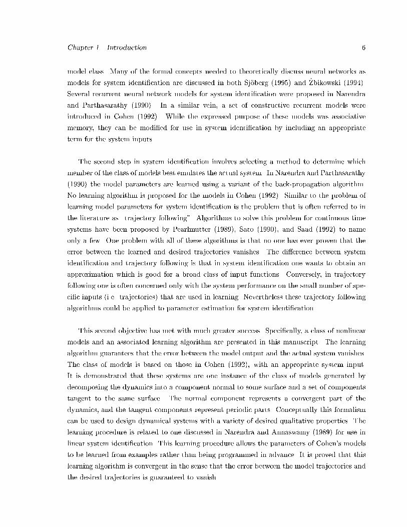
model class� Many of the formal concepts needed to theoretically discuss neural networks as
models for system identi�cation are discussed in both Sj!oberg ������ and �Zbikowski �������
Several recurrent neural network models for system identi�cation were proposed in Narendra
and Parthasarathy ������� In a similar vein� a set of constructive recurrent models were
introduced in Cohen ������� While the expressed purpose of these models was associative
memory� they can be modi�ed for use in system identi�cation by including an appropriate
term for the system inputs�
The second step in system identi�cation involves selecting a method to determine which
member of the class of models best emulates the actual system� In Narendra and Parthasarathy
������ the model parameters are learned using a variant of the back�propagation algorithm�
No learning algorithm is proposed for the models in Cohen ������� Similar to the problem of
learning model parameters for system identi�cation is the problem that is often referred to in
the literature as �trajectory following� Algorithms to solve this problem for continuous time
systems have been proposed by Pearlmutter ������� Sato ������� and Saad ������ to name
only a few� One problem with all of these algorithms is that no one has ever proven that the
error between the learned and desired trajectories vanishes� The di�erence between system
identi�cation and trajectory following is that in system identi�cation one wants to obtain an
approximation which is good for a broad class of input functions� Conversely� in trajectory
following one is often concerned only with the system performance on the small number of spe�
ci�c inputs �i�e� trajectories� that are used in learning� Nevertheless these trajectory following
algorithms could be applied to parameter estimation for system identi�cation�
This second objective has met with much greater success� Speci�cally� a class of nonlinear
models and an associated learning algorithm are presented in this manuscript� The learning
algorithm guarantees that the error between the model output and the actual system vanishes�
The class of models is based on those in Cohen ������� with an appropriate system input�
It is demonstrated that these systems are one instance of the class of models generated by
decomposing the dynamics into a component normal to some surface and a set of components
tangent to the same surface� The normal component represents a convergent part of the
dynamics� and the tangent components represent periodic parts� Conceptually this formalism
can be used to design dynamical systems with a variety of desired qualitative properties� The
learning procedure is related to one discussed in Narendra and Annaswamy ������ for use in
linear system identi�cation� This learning procedure allows the parameters of Cohens models
to be learned from examples rather than being programmed in advance� It is proved that this
learning algorithm is convergent in the sense that the error between the model trajectories and
the desired trajectories is guaranteed to vanish�
Chapter �� Introduction �
The remainder of this dissertation is structured as follows� All of the work done in this
dissertation is based on the mathematical framework of dynamics� Speci�cally� all of the models
considered here are ordinary di�erential equations� Much of the machinery in dynamics is for
the purpose of analyzing the eventual behavior of the solutions to di�erential equations� and
also analyzing the e�ects of perturbations on these solutions� The machinery needed to study
dynamics is brie"y de�ned and discussed in Chapter �� This chapter also de�nes two special
classes of ordinary di�erential equations� gradient systems and Hamiltonian systems� The
behavior of these two types of systems is easy to understand and their behaviors complement
one another� These two classes of systems form the basis for all the work in this dissertation�
In Chapter � it is shown that the dynamics of many existing neural network models can be
decomposed into the sum of a gradient portion and a Hamiltonian portion� An attempt is
made to analyze all such models in the context of this decomposition� While this can be done
successfully in some cases� it is pointed out that there are unresolved di�culties which prevent
a general analysis at this time� In Chapter � the complementary characteristics of gradient and
Hamiltonian systems are used to synthesize a class of nonlinear models for system identi�cation�
Under certain model restrictions� a learning algorithm is proposed which is proven to converge
to a set of parameters for which the error y�t��y�t�p� between the output of the actual system
and the model output vanishes�
Chapter �
Mathematical Formalism
All models presented in this dissertation consist of sets of �rst�order ordinary di�erential equa�
tions �ODEs�� Any deterministic system which has only one continuous independent variable
can be written as a �possibly in�nite� set of �rst order ODEs� Rather than using arbitrary
types of ODEs� all of the models in this work will be composed of a sum of two speci�c classes
of ODEs� One of these classes is the class of gradient systems� the other the class of Hamilto�
nian systems� Both types of systems have been extensively characterized in the mathematics
literature� and their behavior is easy to understand� Lastly� gradient and Hamiltonian sys�
tems have inherently complementary behavior� allowing arbitrary systems to be decomposed
in terms of only these two system types� In Section ��� of this chapter some de�nitions and
general properties of all ODEs are reviewed� The properties of gradient systems as presented
in Hirsch and Smale ������ are reviewed in Section ���� The intuitive behavior of such systems
will be examined in terms of these properties� Section ��� presents a straightforward extension
of gradient systems� termed gradient�like systems� Sections ��� and ��� mirror Sections ��� and
��� except that the properties of Hamiltonian systems� as discussed in Arnold ������� and their
Hamiltonian�like extensions� are presented�
��� Review of Ordinary Di�erential Equations
The study of systems of ordinary di�erential equations �ODEs� is extremely old� Over the
long history of this topic� some of the greatest minds in science have considered various areas
of this broad �eld� The primary reason for the enduring interest in ODEs is that they model
so many physical phenomena well� For example� all of Newtonian mechanics� the evolution of
populations� and electrical circuit analysis can all be modeled as systems of ODEs� Conversely�
the "ow of heat and the propagation of waves in optics and acoustics� can not be modeled
Chapter �� Mathematical Formalism �
using ODEs� There are numerous books about the mathematical theory of ODEs� two that are
referred to extensively in this dissertation are Arnold ������ and Hirsch and Smale ������� One
goal of much of the analysis of ODEs is to �nd those solutions which are eventually approached
from most initial conditions� Another goal is to determine whether these special solutions retain
this character under small perturbations� These two properties are referred to as stability and
structural stability respectively�
����� Terms from Topology
Before proceeding further� the topological notion of a manifold will be de�ned� The basic
notions from topology needed to understand manifolds are discussed in Appendix A� The set
Rn with the metric DE is called a Euclidean metric space and is denoted by En� A manifold is a
metric space which is locally homeomorphic to En� This sort of metric space is used extensively
in the study of di�erential equations� First it should be pointed out that in this dissertation
the inner product is de�ned as hx�yi � xy y �Pn
i�� xi yi� where xy denotes the transpose of
the vector x� Also the norm is de�ned to be kxk � �jx�jp � jx�jp � � � � � jxnjp��
p for some p
such that � � p � �� For the purposes of the de�nitions and theorems any value of p may
be chosen� while in the examples p � � is assumed� Also� the distance between two points
x�y � Rn is de�ned to be the norm of the di�erence between the points DE�x�y� � kx� yk�which for p � � is called the Euclidean distance measure�
A set M and a metric D � M M � ����� de�ned on that set are a manifold if some
neighborhood of every point in M can be deformed into En without being torn or glued�
For example� �the boundary of� a torus is a ��dimensional manifold� likewise the interior of
a cylinder is a ��dimensional manifold� Roughly speaking a manifold is any set which can
be given a set of n independent coordinates in some neighborhood of every point� These
coordinates actually de�ne a homeomorphism between some neighborhood N of every point
and En� Following Christenson and Voxman ������� a manifold may be formally de�ned as
follows�
Denition ���� A separable metric space �M�D� is a manifold if and only if each point x �Mis contained in a neighborhood N M that is homeomorphic to En�
It is shown in Christenson and Voxman ������ that a separable metric space satis�es both the
Hausdor� condition and the second axiom of countability� As discussed in Arnold ������� these
two conditions are needed to guarantee the global uniqueness of the solutions of any ordinary
di�erential equation de�ned on the manifold� Note that the value of n may be di�erent for
each point x �M� This di�culty can be avoided by choosing the set M to be connected� A set
Chapter �� Mathematical Formalism ��
S is connected if and only if it is not the union of disjoint� proper� open subsets� This formalizes
the intuitive notion that a set consists of only �one piece� If the the set M is connected� then
the manifold de�ned by �M�D� is a connected manifold� It is shown in Spivak ������ that if
M is connected� then the value of n is the same for all x � M� Such a manifold is called an
n�manifold and is denoted Mn� where n is called the dimension of the manifold� A di�erent
notion of connectedness is pathwise connectedness� A set S is pathwise connected if and only
if for each x�y � S there is a continuous function g � ��� �� � S such that g��� � x and
g��� � y� This formalizes the notion that a set is connected if one can move from one point in
the set to some other point in the set without leaving the set� Another useful property for a
manifold to possess is that of compactness� This idea is a generalization of the observation that
the set consisting of the all points in the interval �a� b� is both closed and bounded� Although
there are numerous ways to de�ne compactness� the principal de�nition in Christenson and
Voxman ������ is as follows� A set S is compact if and only if every open cover of S has a
�nite subcover� Note that if S Rn then S is compact if it is both closed and bounded� If
the set M is compact� then the manifold de�ned by �M�D� is a compact manifold� Manifolds
have a number of additional properties which are discussed in Spivak ������� For instance� any
manifold is locally connected� locally compact and locally pathwise connected�
����� De�nition of the Phase Space
In general� the study of ODEs is the study of equations of the form
�x � f�x� t�� �����
where x is an n�element vector consisting of the states of the system� �x denotes the derivative
of the states with respect to the independent variable dxdt � f��� is the function f � X T � Y�
for some X�Y Rn � T R� and t denotes the lone independent variable� This system is called
non�autonomous because f��� depends explicitly on the independent variable t� Throughout
much of this dissertation� the systems that will be considered do not explicitly depend on t� and
the range of the function f��� is assumed to be all of Rn � So most of the systems considered
here have the form
�x � f�x�� �����
where f��� is the function f � X� Rn � This system is called autonomous because f��� has no
explicit dependence on the independent variable t� Note that in many scenarios the independent
variable is time� The space of all n states x is called the phase space� while the space of all
states plus the independent variable t is called the extended phase space� An equivalent way
Chapter �� Mathematical Formalism ��
to view the phase space is as the domain X of the function f���� The function f��� de�nes a
vector �eld in the phase space� This means that the vector f�x� is assigned to every point
x in the phase space� In order to visualize this� picture the directed line segment from x to
x � f�x� being assigned to each point x� The function f��� can be used to de�ne a vector
�eld in the extended phase space by introducing the additional state equation �t � �� This is
called a direction �eld in order to di�erentiate it from the vector �eld in the phase space� In
an autonomous system f��� does not depend on t� hence the direction �eld is the same at all
points on the t axis� Note that this would not be true for a non�autonomous system� which is
why the extended phase space is de�ned at all� A curve which at each of its points is tangent
to a direction �eld� is called an integral curve of that direction �eld�
De�ne the function ��x��t��� t� to be the function ��x��t��� �� � T� X where x��t�� � X Tis a point in the extended phase space called an initial condition� The initial condition x��t��
is usually abbreviated x�� The solutions of Equation ����� are exactly those functions ��x�� t�
for which d�dt � f���x�� t�� for all x� � X and t � T� The image of ��x�� t� for a single initial
condition is called a trajectory �alternately a phase curve� solution curve or orbit� and it exists
in the phase space� The graph of ��x�� t� is an integral curve existing in the extended phase
space� So a solution to an ODE is any function whose graph is an integral curve of the given
direction �eld� If a set of initial conditions is considered� then ��x�� t�� where x� � D X�
de�nes the function � � D T � X which is called the �ow� The "ow is often written as
�t�D� rather than ��D� t�� Conceptually the "ow describes how an initial phase space region
is mapped into a �nal region as the system evolves� The following example illustrates these
ideas�
Example ���� Consider the system��x�
�x�
��
��x�
��� x�
�� �����
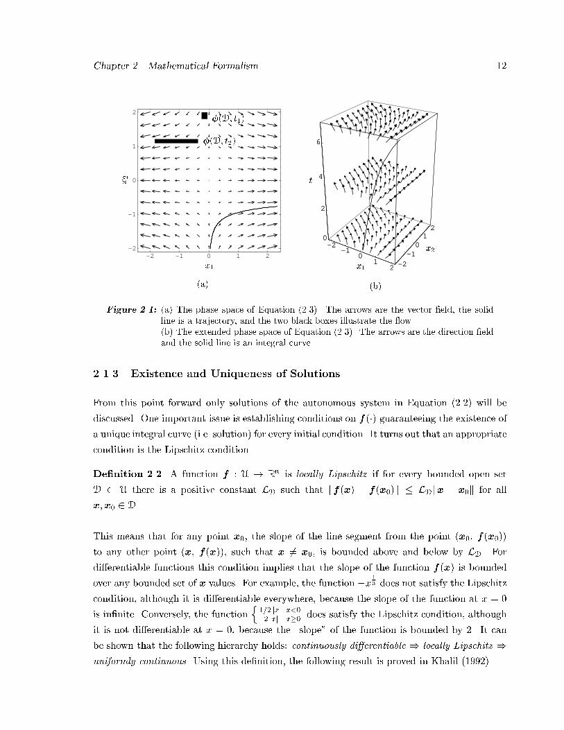
Figure ����a� illustrates the vector �eld� the "ow and a trajectory of this system in the phase
space� Figure ����b� shows the the direction �eld and an integral curve of the system in
the extended phase space� The phase space of this system is R� � while the extended phase
space is R� � The arrows in Figure ����a� are the vector �eld de�ned by the right hand side
of Equation ������ The solid line is an example of a trajectory for this system� The "ow of
the system maps the black square ��D� t�� into the black rectangle ��D� t��� The arrows in
Figure ����b� are the direction �eld de�ned by��x� � �
� x� ��y� Notice that this is equivalent
to introducing the additional state equation �t � �� The solid line is an example of an integral
curve for this system� If this integral curve were projected onto the x��x� plane� the resulting
curve would be identical to the trajectory in Figure ����a��
Chapter �� Mathematical Formalism ��
-2 -1 0 1 2-2
-1
0
1
2
x�
x�
��D� t��
��D� t��
�a�
-2-1
01
2 -2-1012
0
2
4
6
-2-1
01
2 -2-1012
0
2
4
6
x�
x�
t
x�
x�
t
�b�
Figure ���� �a� The phase space of Equation ������ The arrows are the vector �eld� the solidline is a trajectory� and the two black boxes illustrate the �ow��b� The extended phase space of Equation ������ The arrows are the direction �eldand the solid line is an integral curve�
����� Existence and Uniqueness of Solutions
From this point forward only solutions of the autonomous system in Equation ����� will be
discussed� One important issue is establishing conditions on f��� guaranteeing the existence of
a unique integral curve �i�e� solution� for every initial condition� It turns out that an appropriate
condition is the Lipschitz condition�
Denition ���� A function f � U � Rn is locally Lipschitz if for every bounded open set
D U there is a positive constant LD such that kf�x� � f�x��k � LDkx � x�k for all
x�x� � D�
This means that for any point x�� the slope of the line segment from the point �x�� f�x���
to any other point �x� f�x��� such that x �� x�� is bounded above and below by LD� For
di�erentiable functions this condition implies that the slope of the function f�x� is bounded
over any bounded set of x values� For example� the function �x �
� does not satisfy the Lipschitz
condition� although it is di�erentiable everywhere� because the slope of the function at x � �
is in�nite� Conversely� the functionn
��� jxj x���� jxj x��
does satisfy the Lipschitz condition� although
it is not di�erentiable at x � �� because the �slope of the function is bounded by �� It can
be shown that the following hierarchy holds� continuously di�erentiable � locally Lipschitz �uniformly continuous� Using this de�nition� the following result is proved in Khalil �������
Chapter �� Mathematical Formalism ��
Lemma ��� �Local Existence and Uniqueness � Let f�x� be locally Lipschitz� so kf�x��
� f�x��k � LDkx� � x�k for all x��x� � D � fx � Rn � kx � x�k � Kg� Then there exists
some � � � such that the equation �x � f�x� with the initial condition x�t�� � x� has a unique
solution over �t�� t� � ���
This result only applies locally because it is possible for trajectories to leave the regionD after a
�nite time� As a consequence of this restriction� trajectories in phase space can not intersect for
an autonomous system� except at an equilibrium solution� To merely guarantee the existence
of a solution to the equation �x � f�x� for the initial condition x�t�� � x�� continuity of f���su�ces�
����� Equilibrium Solutions
In characterizing the solutions for Equation ������ three types of special solutions are important�
equilibrium solutions� recurrent solutions� and integral manifolds� Equilibrium solutions are
points which have a constant value at all times� As a result� these points are �xed in the phase
space of the system�
Denition ���� A point �x � U such that f��x� � is called an equilibrium point� The set of
all such points in the region U are called the equilibria�
The literature can be confusing because such points are also referred to as �xed points� critical
points� stationary points� singular points� or zeros� For an equilibrium point �x the "ow maps
this point to itself for all time� that is �t��x� � �x for all t � R� If f��� is locally Lipschitz
then the trajectories must eventually converge to or diverge from the equilibrium points at an
exponential or slower rate� As a result� the equilibrium points can not be reached in a �nite
amount of time by any system which satis�es the Lipschitz condition� Some properties and
applications of a class of systems which violate the Lipschitz condition are discussed by Zak
������� Just as converging to or diverging from the equilibria too quickly gives the system
undesirable properties� approaching or retreating too slowly also has unwanted side e�ects� An
equilibrium point for which the rate of approach or retreat is always exponential or greater� is
called hyperbolic�
Denition ���� An equilibrium point �x is hyperbolic if the Jacobian matrix J��x� ��f
�x
�����x
has
no eigenvalue with a zero real part�
Intuitively the Jacobian de�nes the slope of a hyperplane tangent to f��� at the point �x� hence
this condition means that the slope of the hyperplane at the equilibrium point �x is non�zero�
Chapter �� Mathematical Formalism ��
The eigenvalues of the Jacobian for a particular equilibrium point are sometimes called the
characteristic exponents of that point� The sign of the real part of a speci�c eigenvalue deter�
mines whether trajectories converge to or diverge from the equilibrium point in the direction
associated with that eigenvalue� A negative real part indicates convergence� a positive one
divergence� The magnitude of the real part of an eigenvalue gives the rate of convergence or di�
vergence along the associated direction� A large value indicates fast convergence or divergence�
a small value slow convergence or divergence� Note that for a system which is both locally
Lipschitz and has hyperbolic equilibria� the rate of approach or retreat is always exponential�
Another useful notion is that of an isolated equilibrium point� The equilibrium solutions
of any equation �x � f�x� may be of two types� One possibility is that a solution of f�x� �
is a single point in Rn � In this case the solution set contains a single point which is said to be
isolated� The other possibility is that a solution of f�x� � de�nes some larger subset of Rn �
In this case the solution set contains an in�nite number of points and the equilibrium points
are non�isolated� An example of this are the equilibria of the system �r � r�r � �� in polar
coordinates� The point r � � is an isolated equilibrium point of this system� Similarly� every
point on the circle r � � is an equilibrium point� but none of these points are isolated�
Denition ���� An equilibrium point �x is isolated if there exists a neighborhood N � fx �Rn � kx� �xk � Kg of �x such that N contains no equilibria other than �x�
If the Jacobian is non�singular at an equilibrium point �x� then that point is isolated �see for
instance Vidyasagar �������� This means that every hyperbolic equilibrium point is isolated�
The converse of this is not true� Collectively the set of all equilibrium points for a given system
may contain both isolated and non�isolated points�
����� Recurrent Solutions
A trajectory is considered recurrent if it eventually becomes arbitrarily close to its starting
point� This does not mean that it ever returns exactly to the point at which it started�
Following the de�nition in Palis and de Melo ������� this may be formally stated as follows�
Denition ���� A trajectory � is recurrent if � fy � U � �tn�y�� x � � for some sequence
tn � ��g�
A trajectory which eventually returns to its starting point and contains no equilibrium points
is called a closed orbit� Because a closed orbit contains no equilibrium points� the orbit must
continually repeat� However there is not necessarily any regularity to these repetitions�
Chapter �� Mathematical Formalism ��
Denition ���� A trajectory � is a closed orbit if no points in � are equilibrium solutions�
and �t�x� � x for some x � �� and some t �� t��
A trajectory which continually returns to its starting point within some constant time period
is a periodic orbit�
Denition ���� A trajectory � is a periodic orbit if there exists a positive constant T such
that �t�T �x� � �t�x� for all t � R�
It is evident that the following hierarchy holds� periodic orbit � closed orbit � recurrent� It
is shown in Verhulst ������ that if f�x� is locally Lipschitz �i�e� the solutions are unique�� then
a trajectory is a closed orbit if and only if it is a periodic orbit�
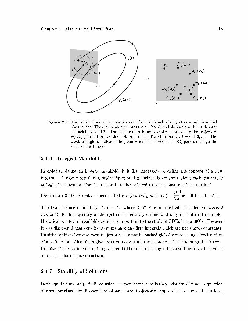
The concept of hyperbolicity can be extended to include closed orbits� To properly de�ne
this requires the notion of a Poincar�e map� Choose an �n � ���dimensional surface S which is
transverse to the "ow �t�S� for every point x� � S� The two subspaces B� and B� of the space
B are transverse if their sum B� � B� is the entire space B� This means that any member
of B can be decomposed into a member of B� and a member of B�� For example� a line
and a plane are transverse in R� if they intersect at a nonzero angle� By contrast� two lines
cannot be transverse in R� � Select a neighborhood N S of the point ��t�� where the closed
orbit intersects the surface S� This construction is illustrated for a ��dimensional phase space
in Figure ���� The Poincar�e map is the function p � N � S� This map returns the points
corresponding to the discrete time values at which the trajectory �t�x�� intersects the surface
S� The point ��t�� is clearly an equilibrium point of p� It is proven in Hirsch and Smale ������
that the behavior of the trajectory �t�x�� with respect to the closed orbit ��t� is identical to
the behavior of the Poincar�e map p with respect to the point ��t���
Denition ���� A closed orbit ��t� is hyperbolic if the Jacobian matrix of the Poincar�e map
p at the equilibrium point ��t��� J�p j��t�� ��p
�x
������t�
has no eigenvalues with a magnitude
of one�
The di�erence in the eigenvalue condition between this de�nition and De�nition ���� is due to
the fact that p is a discrete�time function while f is a continuous�time function� The eigenvalues
of the Jacobian for a particular closed orbit are sometimes called the characteristic multipliers
of the orbit� The magnitude of a speci�c eigenvalue determines whether trajectories converge to
or diverge from the closed orbit in the direction associated with that eigenvalue� A magnitude
less than one indicates convergence� greater than one divergence� Note that there are �n � ��
characteristic multipliers for a closed orbit in an n�dimensional phase space�
Chapter �� Mathematical Formalism ��
�
S
�t�x��
��t�
�t��x��
x�
�t��x���t�
�x��
�t��x�� ��t��
�t��x��
�t��x��
�t��x��x�
S
��t��N
Figure ���� The construction of a Poincare map for the closed orbit ��t� in a ��dimensionalphase space� The gray square denotes the surface S� and the circle within it denotesthe neighborhood N� The black circles � indicate the points where the trajectory�t�x�� passes through the surface S at the discrete times ti� i �� � �� � � � � Theblack triangle N indicates the point where the closed orbit ��t� passes through thesurface S at time t��
����� Integral Manifolds
In order to de�ne an integral manifold� it is �rst necessary to de�ne the concept of a �rst
integral� A �rst integral is a scalar function I�x� which is constant along each trajectory
�t�x�� of the system� For this reason it is also referred to as a �constant of the motion�
Denition ���� A scalar function I�x� is a �rst integral if �I�x� ��I
�x
y�x � � for all x � U�
The level surface de�ned by I�x� � K� where K � R is a constant� is called an integral
manifold� Each trajectory of the system lies entirely on one and only one integral manifold�
Historically� integral manifolds were very important to the study of ODEs in the ����s� However
it was discovered that very few systems have any �rst integrals which are not simply constants�
Intuitively this is because most trajectories can not be packed globally onto a single level surface
of any function� Also� for a given system no test for the existence of a �rst integral is known�
In spite of these di�culties� integral manifolds are often sought because they reveal so much
about the phase space structure�
���� Stability of Solutions
Both equilibrium and periodic solutions are persistent� that is they exist for all time� A question
of great practical signi�cance is whether nearby trajectories approach these special solutions�
Chapter �� Mathematical Formalism ��
this is precisely the issue of stability� Broadly speaking� an equilibrium point is stable if
trajectories starting nearby remain nearby at all future times� The following formal de�nition
is given in Arnold �������
Denition ����� The equilibrium point �x is stable if for every � � there exists ��� � � such
that for every initial condition x� for which kx�� �xk � ���� the trajectory �t�x�� satis�es the
inequality k�t�x��� �t��x�k � for all t � t��
Note that since �x is an equilibrium point� by de�nition �t��x� � �x� An equilibrium point
is asymptotically stable if trajectories starting nearby not only remain nearby but eventually
become arbitrarily close to the equilibrium point�
Denition ����� The equilibrium point �x is asymptotically stable if it is stable and if limt��
�t�x�� � �t��x� for all x� such that kx� � �xk � ����
An equilibrium point is unstable if at least one trajectory starting arbitrarily nearby ceases to
be nearby at some time� This does not mean that the trajectory is always far away from the
equilibrium point or even that it can not be frequently close�
Denition ����� The equilibrium point �x is unstable if there exists an � � such that for
every ��� � � there exists an initial condition x� for which kx� � �xk � ���� whose trajectory
�t�x�� satis�es the inequality k�t�x��� �t��x�k � for some t � t��
While intuitively pleasing� the above de�nitions of stability require explicit knowledge of the
solutions of a system in order to determine the stability of its equilibrium points� For most
ODEs explicit solutions are unknown� so some other method must be used to determine the
stability of the equilibria�
One way to proceed is to linearize the system about a speci�c equilibrium point and then
analyze the stability of the linear system� This requires rewriting the system as �x � J��x� �x��x��O�kx� �xk�� where J��x� is the Jacobian matrix de�ned in De�nition ��� at the equilibrium
point �x� The notation O�kx � �xk�� indicates that the expression for the dynamics contains
higher order terms h�x�� such that limkx��xk��kh�x��xkkx��xk� � K� where K is a non�negative
constant� If limkx��xk��O�kx��xk�kx��xk � � then there exists some neighborhood of �x in which
�x � J��x� �x � �x� � f�x�� The assumption embodied by the above limit is valid if f�x� is
continuously di�erentiable in some neighborhood of the point �x� This does not mean that the
"ow of the linear system bears any resemblance to that of the nonlinear system� However� if
the equilibrium point is hyperbolic� then it has been proven that the "ows of the linear and
nonlinear systems are qualitatively similar�
Chapter �� Mathematical Formalism ��
The Hartman�Grobman Theorem �Guckenheimer # Holmes� ����� states that if an equilib�
rium point is hyperbolic� then in some neighborhood of this point there is a homeomorphism�
which locally takes the trajectories of the nonlinear system �x � f�x� to those of the linear
system �x � J��x� �x� �x�� The homeomorphism preserves the sense of the trajectories and can
be chosen to preserve the parametrization by the independent variable t� It turns out that the
similarities between the linear and nonlinear "ow are even greater than this� To quantify this�
the concepts of stable and unstable manifolds must be de�ned� The stable manifold in some
neighborhood of the equilibrium point �x consists of all points which lie on trajectories which
approach �x as t � � in such a way that the trajectory never leaves the neighborhood� The
points on trajectories which approach �x in this manner as t � �� constitute the unstable
manifold of �x�
Denition ����� The local stable manifold Wsloc��x� in the neighborhood N of the equilibrium
point �x is the set Wsloc��x� � fx� � N � �t�x�� � �x as t � �� and such that �t�x�� � N
for all t � t�g� Similarly� the local unstable manifold Wuloc��x� is the set Wu
loc��x� � fx� � N �
�t�x��� �x as t� ��� and such that �t�x�� � N for all t � t�g�
The Stable Manifold Theorem �Guckenheimer # Holmes� ����� states that if an equilibrium
point is hyperbolic then the local stable and unstable manifolds of the nonlinear system
�x � f�x� have the same dimensions as those of the linear system �x � J��x� �x � �x�� Fur�
thermore� the stable and unstable manifolds of the nonlinear system are tangent to those of the
linear system at �x� The global stable manifoldWs contains all points lying on trajectories which
eventually become part of the local stable manifold� in other wordsWs��x� �S
t�t� �t�Wsloc��x���
Similarly the global unstable manifold is de�ned as Wu��x� �S
t�t� �t�Wuloc��x��� If f��� sat�
is�es the Lipschitz condition� then two stable �or unstable� manifolds associated with distinct
equilibrium points �x�� �x� can not intersect� nor can a stable �or unstable� manifold intersect
itself� However� intersections of the stable and unstable manifolds of distinct equilibria� or even
the same equilibrium point can occur�
Together these two results mean that the stability of any hyperbolic equilibrium point �x
can be determined by �nding the eigenvalues of the Jacobian J��x�� If the eigenvalues of the
Jacobian J��x� all have strictly negative real parts then the equilibrium point is asymptotically
stable� Likewise if any of the eigenvalues of J��x� have a positive real part then the equilibrium
point is unstable� This leads to the notion of the index of an equilibrium point�
Denition ����� The index of a vector �eld f at an equilibrium point �x is the dimension of
the subspace spanned by the eigenvectors of the Jacobian J��x� whose corresponding eigenvalues
have positive real part�
Chapter �� Mathematical Formalism ��
Conceptually the index is the dimension of the subspace containing all trajectories which are
repelled from the equilibrium point� Therefore by de�nition� the index is the dimension of the
unstable manifold� For example� in ��dimensions the index of a stable point �i�e� a sink� is
�� that of a saddle point is �� and that of an unstable point �i�e� a source� is �� Using these
results it is proven in Hirsch and Smale ������ that a hyperbolic equilibrium point must be
either asymptotically stable or unstable� It should be noted that an equilibrium point may be
asymptotically stable or unstable without the Jacobian satisfying these conditions� An example
of this behavior is the system �x � �x�� The origin of this system is asymptotically stable� but
the eigenvalue of the Jacobian at the origin is zero� Another interesting example is the system
�x� � x�� �x� � �x�� � x�� The origin of this system is unstable although the eigenvalues of the
Jacobian at the origin are � and ���
These concepts of stability can be extended to periodic solutions� A periodic orbit is stable
if trajectories starting in some neighborhood remain in a neighborhood� and in addition points
in phase space which start out close together remain near each other� This means that all
trajectories near the periodic orbit must have periods which are similar in some sense� It
should be noted that most periodic orbits are not stable�
Denition ����� A periodic orbit ��t� is stable if for every � � there exists ��� � � such
that for every initial condition x� for which kx�� ��t��k � ���� the trajectory �t�x�� satis�es
the inequality k�t�x��� ��t�k � for all t � t��
A periodic orbit is asymptotically stable if trajectories starting nearby not only remain nearby
but eventually become arbitrarily close to the periodic orbit� Note that if the system of ODEs
is locally Lipschitz� a trajectory in a neighborhood of a periodic orbit can never reach any
point on the periodic orbit� Any such point on the periodic orbit would have to be either
an equilibrium solution� which violates the de�nition of a periodic orbit� or a point where
uniqueness of the solutions breaks down� which can not occur in a locally Lipschitz system� So
trajectories near an asymptotically stable periodic orbit eventually become arbitrarily close to
the periodic orbit� but can never actually reach it�
Denition ����� The periodic orbit ��t� is asymptotically stable if it is stable and if limt��
k�t�x��� ��t�k � � for all x� such that kx� � ��t��k � ����
It is proven in Hirsch and Smale ������ that for an asymptotically stable periodic orbit �� with
period T � there exists a neighborhoodN U such that for every point x� � N� limt��k�t�T �x���
�t�x��k � �� This means that eventually all trajectories near an asymptotically stable periodic
orbit behave as if they had the same period as the periodic orbit� Note that this does not mean
Chapter �� Mathematical Formalism ��
that the nearby trajectories are ever in�phase with the periodic orbit� The following example
illustrates the di�erences between these ideas�
Example ���� Consider the following three systems�
�x� � x�
�x� � � sinx�Pendulum Oscillator �����
�x� � x�
�x� � �x�Harmonic Oscillator �����
�x� � x�
�x� � �x� � x���� x��
� � � van der Pol Oscillator �����
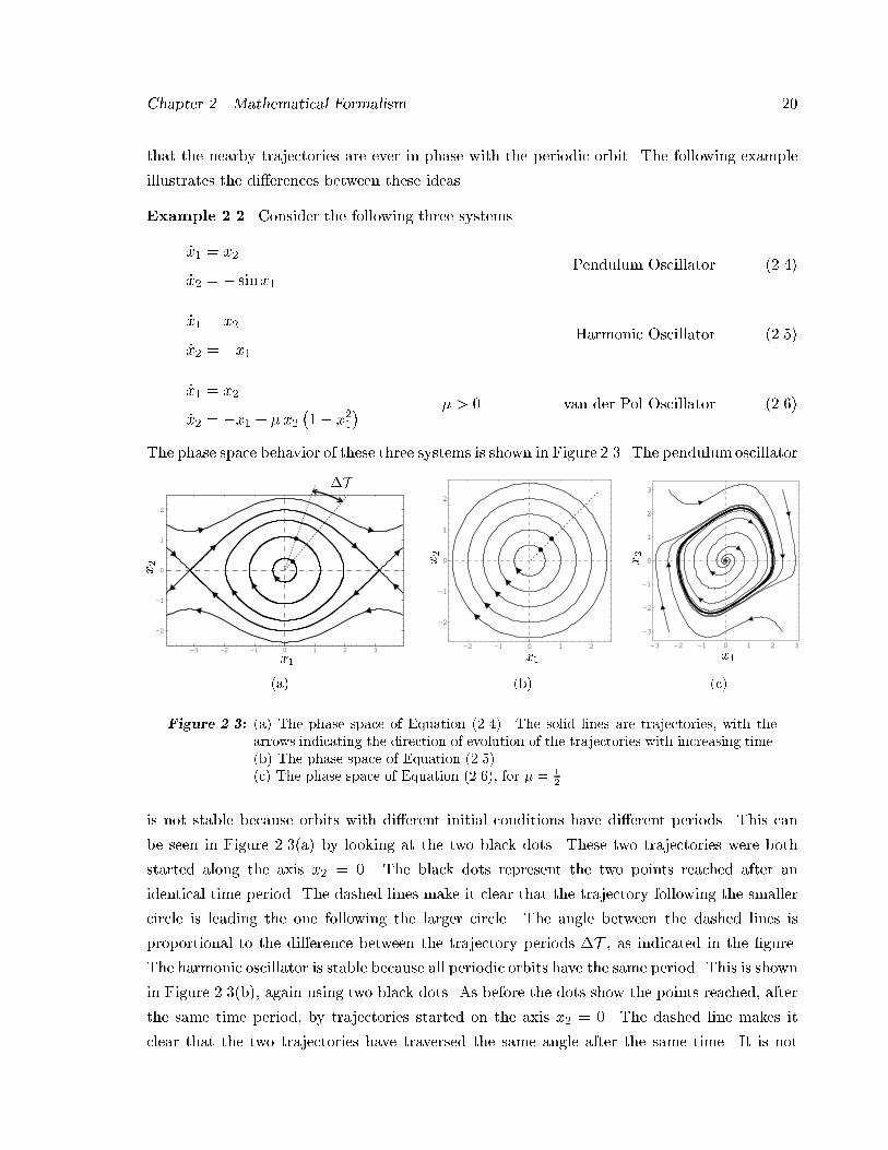
The phase space behavior of these three systems is shown in Figure ���� The pendulum oscillator
-3 -2 -1 0 1 2 3
-2
-1
0
1
2
x�
x�
�T
�a�
-2 -1 0 1 2
-2
-1
0
1
2
x�
x�
�b�
-3 -2 -1 0 1 2 3
-3
-2
-1
0
1
2
3
x�
x�
�c�
Figure ���� �a� The phase space of Equation ������ The solid lines are trajectories� with thearrows indicating the direction of evolution of the trajectories with increasing time��b� The phase space of Equation �������c� The phase space of Equation ������ for � �
� �
is not stable because orbits with di�erent initial conditions have di�erent periods� This can
be seen in Figure ����a� by looking at the two black dots� These two trajectories were both
started along the axis x� � �� The black dots represent the two points reached after an
identical time period� The dashed lines make it clear that the trajectory following the smaller
circle is leading the one following the larger circle� The angle between the dashed lines is
proportional to the di�erence between the trajectory periods $T � as indicated in the �gure�
The harmonic oscillator is stable because all periodic orbits have the same period� This is shown
in Figure ����b�� again using two black dots� As before the dots show the points reached� after
the same time period� by trajectories started on the axis x� � �� The dashed line makes it
clear that the two trajectories have traversed the same angle after the same time� It is not
Chapter �� Mathematical Formalism ��
asymptotically stable because for a speci�c periodic orbit� nearby trajectories do not approach
this orbit� In fact� for this system all trajectories are periodic orbits� The van der Pol oscillator�
shown in Figure ����c�� contains a single asymptotically stable periodic orbit�
The de�nitions of stable and unstable manifolds can easily be extended to closed orbits by
considering all points on trajectories which approach the orbit � in such a way that they never
leave some neighborhood of �� In this case the stable and unstable manifolds are denoted
Ws��� and Wu��� respectively�
���� Asymptotic Behavior of Solutions
Analyzing the long term behavior of a system of ODEs is an issue that is extremely important�
In this subsection various types of limit sets are de�ned to facilitate this analysis� Equilibrium
points represent solutions which are stationary in the phase space for all time� Similarly�
periodic orbits are also stationary in that the orbit as a unit does not move in the phase space�
A generalization of both these ideas is an invariant set�
Denition ����� The set I U is an invariant set if for every point x� � I then �t�x�� � Ifor all t � R�
If this de�nition applies only for t � t�� then I is called a positive invariant set� and if it is true
only for t � t�� I is a negative invariant set� Equilibrium points� closed orbits� and integral
manifolds are all examples of invariant sets� In many systems it turns out that the "ow does
not approach many of the members of the invariant set� In fact many points in the invariant
set represent only the transient behavior of the system� For this reason� other more exclusive
concepts have been developed�
In studying the asymptotic behavior of a system it is natural to try to �nd the points that
all trajectories go to and come from� This is the idea behind the concept of limit sets� The
��limit set of a point x� is the set of all points q which the trajectory starting at x� approaches
as t � �� The ��limit set of x� is the set of all points q which the trajectory starting at x�
approaches as t � ��� From Hirsch and Smale ������ the de�nition of the ��limit set is as
follows�
Denition ����� A point q is an ��limit point of the trajectory �t�x�� if there exists a se�
quence tn �� such that limtn���tn�x��� q� The ��limit set of x�� denoted L��x��� is the
set of all ��limit points q� of the trajectory associated with the initial condition x��
Letting the sequence be tn � �� in the previous de�nition yields the de�nition of an ��limit
set� denoted L��x��� The point q is an ��limit point if the distance between q and at least one
Chapter �� Mathematical Formalism ��
trajectory eventually becomes arbitrarily small� These de�nitions can readily be generalized to
a closed orbit �� as in Hirsch and Smale �������
Denition ���� A trajectory � is an ��limit cycle if � is closed orbit and there exists some
point x� �� � such that � L��x���
Conceptually� if at least one trajectory� other than the closed orbit itself� eventually becomes
arbitrarily close to a closed orbit� then the closed orbit is an ��limit cycle� This condition is
weaker than asymptotic stability� since asymptotic stability requires all trajectories in some
neighborhood of the closed orbit to eventually become arbitrarily close� Replacing the ��limit
set L��x�� in this de�nition by the ��limit set L��x��� gives the de�nition for an ��limit cycle�
It is proven in Hirsch and Smale ������ that the limit sets L���� and L���� are always closed�
invariant sets� If the limit set is bounded� then in addition to the above it is also connected
and non�empty�
It is also natural in analyzing the long term behavior to �nd those points which represent
repetitious behaviors of the system� This is the idea behind the nonwandering set� Intuitively�
a nonwandering point lies on or near trajectories which eventually return to within a speci�
�ed distance of themselves� The set of all such points is the nonwandering set� As given in
Guckenheimer and Holmes ������� the mathematical de�nition of the nonwandering set is as
follows�
Denition ����� A point q is nonwandering for the "ow �t��� if for every neighborhood N
of q and some T � � there exists some t � T for which �t�N� � N �� �� The set of all such
points for all x� � U is the nonwandering set Z�f� for the vector �eld f �
Notice that �t�N� is the set of all solution states at time t which have initial conditions x� � N�
So the point q is a nonwandering point if at least one trajectory started in the neighborhood N�
returns to N at some later time� For example� if q is a point on an unstable periodic orbit� only
one trajectory from any neighborhood of q returns to that neighborhood� but this is su�cient
to make q a nonwandering point� Like the limit sets� it is proven in Palis and de Melo ������
that the nonwandering set Z�f� is a closed invariant set� Additionally it has been shown that
Z�f� L��f��L��f� and that in particular Z�f� always contains the equilibrium points and
closed orbits of the system�
One of the most natural ways to analyze a dynamical system� is to look for a set of points
which is approached by a large number of trajectories� This intuitive idea is the basis for
trying to de�ne an attractor� For some technical reasons� creating a general de�nition for
this apparently simple concept has proven quite di�cult� There does not appear to be one
Chapter �� Mathematical Formalism ��
de�nition which is satisfactory in all cases� The following de�nition from Guckenheimer and
Holmes ������ de�nes a set which eventually captures all trajectories starting in some domain�
Denition ����� The set A is an attracting set if A is a closed invariant set� and there exists
some neighborhoodN U containing A� such that for all x� � N� the trajectory �t�x�� � N for
all t � t�� and limt���t�x��� A� The set of all points lying on trajectories which eventually
enter the neighborhood N� in other wordsS
t�t� �t�N�� is the domain of attraction of A�
It should be noted that there are many circumstances in which this de�nition leads to an
attracting set which runs counter to ones intuitive de�nition of an attractor�
The following example illustrates these sets and clari�es the di�erence between a nonwan�
dering point and a limit point�
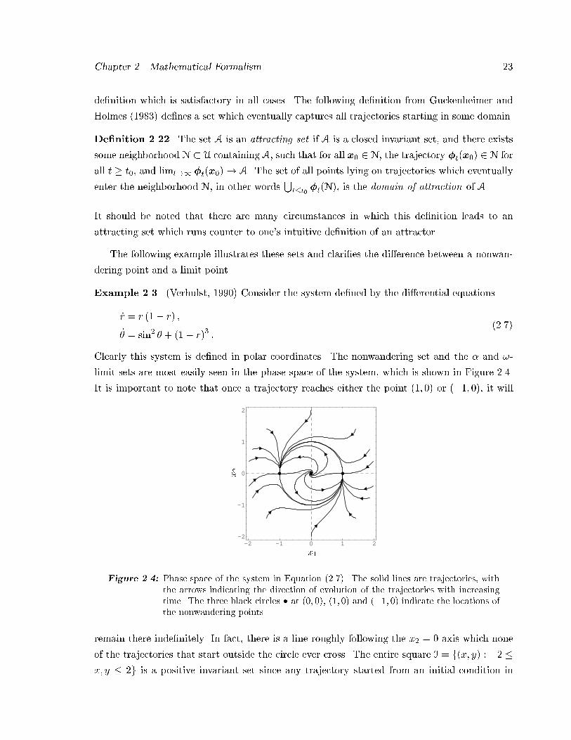
Example ���� �Verhulst� ����� Consider the system de�ned by the di�erential equations
�r � r ��� r� �
� � sin� � ��� r�� ������
Clearly this system is de�ned in polar coordinates� The nonwandering set and the � and ��
limit sets are most easily seen in the phase space of the system� which is shown in Figure ����
It is important to note that once a trajectory reaches either the point ��� �� or ���� ��� it will
-2 -1 0 1 2-2
-1
0
1
2
x�
x�
Figure ���� Phase space of the system in Equation ������ The solid lines are trajectories� withthe arrows indicating the direction of evolution of the trajectories with increasingtime� The three black circles � at ��� ��� � � �� and �� � �� indicate the locations ofthe nonwandering points�
remain there inde�nitely� In fact� there is a line roughly following the x� � � axis which none
of the trajectories that start outside the circle ever cross� The entire square I � f�x� y� � �� �x� y � �g is a positive invariant set since any trajectory started from an initial condition in
Chapter �� Mathematical Formalism ��
I always remains in I for all increasing time� The circle r � � is an invariant set since any
trajectory started on it remains on it for all time� The origin is the only ��limit point of the
system because all points inside the circle r � � lie on a trajectory which gets arbitrarily close
to the origin after an arbitrarily long negative time� The circle r � � is the ��limit set for every
point in the plane� except the origin� because all points lie on a trajectory which gets arbitrarily
close to some portion of the circle after an arbitrarily long positive time� The nonwandering
set contains the points ��� ��� ��� �� and ���� �� because only trajectories started at these three
points will eventually return to these points� The three black dots in Figure ��� mark the
locations of the nonwandering points� So any trajectory started on r � � will eventually leave
the neighborhood of the starting point and not return� with the exception of trajectories started
at ��� �� and ���� ��� The circle r � � is also an attracting set whose domain of attraction is
all of R� with the exception of the origin�
As this example shows the nonwandering set and the limit set L��f� � L��f� do not have to
contain the same elements� The fundamental di�erence between limit points and nonwandering
points is that while a limit point is a point which at least one trajectory eventually becomes
arbitrarily close to� a nonwandering point is a point which at least one trajectory� started nearby �
eventually becomes arbitrarily close to� No idea of recurrence is embodied in the de�nition of
a limit point� while it is fundamental to the de�nition of a nonwandering point� Also notice
that in this example most of the points in the attracting set are wandering� which is somewhat
counter�intuitive�
����� Lyapunov Stability
Another way to determine the stability of equilibria which will be used extensively in this
dissertation� is the method due to the mathematician Lyapunov� The idea behind Lyapunov
stability is to choose a scalar function W�x�� with closed level surfaces �i�e� surfaces such that
W�x� � K for some K � R�� in such a way that the trajectories of the system in Equation �����
always move toward level surfaces with smaller values of K� In addition� as the value of Kdecreases� the size of the associated level surface also decreases� So once the trajectory crosses
the surface W�x� � K into the set CK � fx � Rn � W�x� � Kg� it never leaves that set� and
it moves toward sets with smaller K values� As K decreases the surface W�x� � K shrinks to
the equilibrium point �x� hence the trajectory approaches �x as time increases� Formally this is
stated in the following lemma taken from Hirsch and Smale �������
Lemma ��� �Lyapunov � Let �x � U be an equilibrium point of Equation ������ Let W �
U � R be a continuous function which is de�ned on some neighborhood N U of �x� is

Chapter �� Mathematical Formalism ��
di�erentiable on N n �x� and has the property that �� W��x� � � and W�x� � � for all x �� �x�
If �� �W�x� � rxWy �x � � for all x in N n �x� then �x is stable� Furthermore� if �� �W�x� � �
for all x in N n �x� then �x is asymptotically stable�
Any function satisfying �� is said to be positive de�nite� A function W�x� with properties��
and �� is called a Lyapunov function for the equilibrium point �x� If property �� also holds
thenW�x� is a strict Lyapunov function� Note that Lyapunovs method can be applied without
solving the di�erential equations� On the other hand� there is no constructive technique for
�nding a Lyapunov function for an arbitrary system�
There are several di�culties with applying this theorem in many situations� First� in order
to prove asymptotic stability it is necessary to �nd a positive de�nite function whose time
derivative is always negative de�nite� This may be extremely di�cult� Second� this method
can not be used to analyze the global stability of systems with more than one equilibrium
point� Furthermore� it can not be used to determine the stability of systems with non�isolated
equilibria at all� Third� this procedure gives no indication of the size of the region of attraction
of an equilibrium point� All of these di�culties are surmounted by the following lemma� proved
in LaSalle and Lefschetz �������
Lemma ��� �LaSalle � Let D be a compact set such that for every initial condition x� � D�the corresponding trajectory �t�x�� of Equation ����� remains in D for all t � t�� Let W �
D � R be a continuously di�erentiable function such that �W�x� � � for all x � D� Let G be
the set of all points in D where �W�x� � �� Let A be the largest invariant set in G� Then every
trajectory starting in D approaches A as t���
Note that the construction of the set D does not necessarily depend on the construction of the
function W�x�� The set D is an estimate of the region of attraction of the attracting set A�
Since it su�ces that �W�x� � � for all x � D� this method can be used to analyze the global
stability of systems with multiple equilibria or systems with non�isolated equilibria� Since the
set A is not required to contain equilibrium points� this theorem can be extended to show the
stability of periodic orbits� as shown in LaSalle �������
������ Structural Stability
A vector �eld is structurally stable if the signi�cant features of the phase space remain un�
changed by the addition of a su�ciently small vector �eld� More speci�cally� a vector �eld is
structurally stable if the direction in which points "ow along the trajectories as time increases�
and the way in which trajectories approach the equilibrium solutions and closed orbits� remains
Chapter �� Mathematical Formalism ��
the same in the presence of su�ciently small perturbations� For example� an equilibrium point
that trajectories are diverging from along a spiral path� will remain so for a small enough
perturbation of the vector �eld� Hence a system having one equilibrium point of this type is
structurally stable�
A brief review of the mathematical history of structural stability follows� It was proven
in Peixoto ������ that structural stability was a generic property of systems on ��dimensional
manifolds� This means that a randomly chosen ��dimensional system has an in�nitely small
probability of not being structurally stable� Therefore almost all ��dimensional systems are
structurally stable� This very convenient property was shown not to extend to systems on
manifolds with dimension � � in Smale ������ and then to systems with dimension � in
Newhouse ������� Although structural stability is not generic on manifolds with dimension
� �� a class of vector �elds which are always structurally stable was presented in Palis and
Smale ������� This class of vector �elds� called Morse�Smale� is de�ned as follows�
Denition ����� Let Mn be a compact manifold of dimension n� Let f � Cr be a vector �eld
de�ned on Mn� f is a Morse�Smale vector �eld if� �� the equilibrium solutions and closed
orbits of f are all hyperbolic� and are �nite in number� �� if �� and �� are any two distinct
equilibrium solutions or closed orbits of f � then the stable manifold Ws���� is transverse to
the unstable manifold Wu����� �� the nonwandering set Z�f� is equal to the union of the
equilibrium solutions and closed orbits of f �
The stable and unstable manifolds are discussed in De�nition ����� The nonwandering set Z�f�
is discussed in De�nition ����� It is proven in Palis and Smale ������ that if a vector �eld is
Morse�Smale� then it is structurally stable� The converse of this result is not true�
��� Properties of Gradient Systems
A gradient system is one in which the time derivative of the states �x depends on the partial
derivatives of a scalar function V�x�� Intuitively� the behavior of gradient systems can be
understood by realizing that the state of the system may only move downward along the
surface of V�x� following the line of steepest descent� The function V�x�� called the gradient
potential function� is a mapping of the form V � U� R� such that V � C� and where U is an
open set such that U Rn � Gradient dynamics are described by the equation
�x � �rxV�x� � f�x��
�
��x� �x� � � � �xn
y� �
��V
�x�
�V
�x�� � � �V
�xn
�y�
�����
Chapter �� Mathematical Formalism ��
Since rxV�x� is continuously di�erentiable� it is locally Lipschitz� hence this system has a
unique solution for every initial condition in U� This class of systems has been extensively
studied in the mathematics literature� and all of the results presented in this section are proved
elsewhere� Theorems ���� ���� ��� and ���� and Corollary ��� are proven in Hirsch and Smale
������� Theorems ��� and ��� in Palis and Smale ������� and Theorem ��� in Khalil �������
The �rst theorem and its corollary show that trajectories always move toward smaller values
of V�x�� The only exception to this is at equilibrium points where a trajectory must remain
constant�
Theorem ���� �V�x� � � for all x � U and �V�x� � � if and only if x is an equilibrium point
of Equation ������
Theorem ��� can be used to prove the following corollary�
Corollary ���� If %x is an isolated minimum of V�x� then %x is an asymptotically stable equi�
librium point of Equation ������
Notice that not every equilibrium point of Equation ����� is a local minimum of V�x�� However�
the previous two results show that every isolated local minimum of V�x� is an asymptotically
stable equilibrium point of Equation ������ This means that if a trajectory starts within some
neighborhood of %x� eventually it will reach %x� This is a purely local result� and it does not
guarantee that every trajectory will converge to some equilibrium point� The next theorem
gives a geometric description of the "ow of the gradient system�
Theorem ���� For a gradient system the trajectories at regular points �i�e� points where
�V�x� �� �� are normal to the level surfaces of V�x� �i�e� surfaces where V�x� � K� K � R��
Non�regular points are equilibria of the system�
This is a formal statement of the intuitive behavior of the system that was made previously�
The trajectories of a gradient system can only remain constant at an equilibrium point and
must move toward smaller values of V�x� at all other points� This implies that for a gradient
system� only a trajectory started at an equilibrium point is recurrent� Trajectories started at
all other points will move away from those points and not return� Theorem ��� identi�es the
recurrent trajectories in terms of the nonwandering set� which was de�ned in De�nition �����
Theorem ���� The nonwandering set Z�f� for a gradient system contains only the equilibrium
points of the system�
Theorem ��� states that eventually� the only recurrent trajectories in the phase space are the
equilibrium points� This theorem implies that eventually a gradient system has no recurrent
Chapter �� Mathematical Formalism ��
trajectories� Intuitively� this behavior would require that the system be able to move both up
and downhill along V�x�� or remain at arbitrary values of V�x�� neither of which can occur in
a gradient system�
All trajectories of a gradient system must move downhill along V�x�� Therefore all trajec�
tories must approach a stable equilibrium point or go to in�nity� Likewise all trajectories must
begin near an unstable equilibrium point or at in�nity� Theorem ��� identi�es these asymptotic
trajectories in phase space as t� �� in terms of � and ��limit sets� de�ned in De�nition �����
Theorem ���� If the point �x is an � or ��limit point of any trajectory of a gradient system�
then �x is an equilibrium point of the system�
This theorem implies that if the equilibrium points are isolated� then the solution state must
either go to an equilibrium point or to in�nity� Note that in�nity can not be a member of
either the � or ��limit sets� For a gradient system the nonwandering set and the union of the
� and ��limit sets are both equal to the same set� namely the set of equilibrium points� In
general this is not the case�
The next theorem states the conditions under which all trajectories will go to some equi�
librium point�
Theorem ���� Consider the dynamical system given by Equation ������ Suppose that the set
CK � fx � Rn � V�x� � Kg �����
is compact for every K � R� Then every solution of the system x�t� is de�ned for all t � ��
Suppose that the system has a �nite number of isolated equilibrium points q�� q�� � � � � qe�
Then for every solution x�t�� limt�� x�t� exists and equals one of the equilibrium points�
There are many possible ways to constrain V�x� so that the set CK is compact� One way is to
make V�x� lower bounded� V�x� � Bl for all x � R� and radially unbounded� limkxk��V�x����
Not only is the set of orbits which the trajectories can approach restricted but the way in
which those orbits are approached is also limited� This is shown in Theorem ����
Theorem ���� At every equilibrium point �x of Equation ������ the linearized system �x �
JG��x� �x� �x� has real eigenvalues� The Jacobian JG��x� is
Chapter �� Mathematical Formalism ��
JG��x� ��f�x�
�x
�����x
���V
�x�
�����x
� ������
Furthermore� JG��x� is diagonalizable and its eigenvectors form a complete orthonormal set�
In this dissertation� an improper node is de�ned as any equilibrium point where the Jacobian
is not diagonalizable� Since JG��x� is always diagonalizable� no improper nodes exist for a
gradient system� Because the eigenvalues of JG��x� are real� only three types of equilibrium
points are possible� a proper stable point �i�e� a sink�� a proper unstable point �i�e� a source��
or a saddle point� Conceptually this means that within a small enough neighborhood of any
equilibrium point� the shape of any trajectory must be a hyperbola� a parabola� or a line� For a
general discussion of equilibrium point analysis in nonlinear systems see Verhulst ������� Note
that the Jacobian of the system JG�x� is equivalent to the Hessian of the potential function��V�x�
� So the Jacobian describes the curvature of the potential function�
It was stated previously that structural stability is not a generic property of systems whose
phase space is a manifold with dimension � or higher� An exception to this was shown in
Palis and Smale ������� where it was demonstrated that almost all possible gradient systems
are structurally stable regardless of manifold dimension� The following theorem gives the
conditions under which a gradient system is structurally stable�
Theorem ���� A gradient system is structurally stable if and only if every equilibrium point
is hyperbolic and all stable and unstable manifolds intersect transversally�
For a gradient system any equilibrium point which is isolated is also hyperbolic� This is not
true for most other systems� Notice that the two conditions given are necessary and su�cient�
hence every structurally stable gradient system must satisfy the de�nition of a Morse�Smale
system�
All of this means that knowing the locations of the minima of the potential function V�x�
almost completely characterizes a gradient system� This is due to the fact that almost all
trajectories will eventually reach one of these points and then remain their inde�nitely�
��� Properties of Gradient�Like Systems
All of the useful properties of gradient systems are also possessed by a more general class of
dynamical systems� which will be referred to as gradient�like systems� Gradient�like system
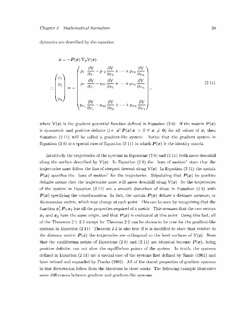
Chapter �� Mathematical Formalism ��
dynamics are described by the equation
�x � �P �x�rxV�x��
�
BBBBB�
�x�
�x����
�xn
�CCCCCA � �
BBBBBBBBBBB�
p���V
�x�� p��
�V
�x�� � � �� p�n
�V
�xn
p���V
�x�� p��
�V
�x�� � � �� p�n
�V
�xn���
pn��V
�x�� pn�
�V
�x�� � � �� pnn
�V
�xn
�CCCCCCCCCCCA�
������
where V�x� is the gradient potential function de�ned in Equation ������ If the matrix P �x�
is symmetric and positive de�nite �i�e� xyP �x�x � � � x �� � for all values of x� then
Equation ������ will be called a gradient�like system� Notice that the gradient system in
Equation ����� is a special case of Equation ������ in which P �x� is the identity matrix�
Intuitively the trajectories of the systems in Equations ����� and ������ both move downhill
along the surface described by V�x�� In Equation ����� the �laws of motion state that the
trajectories must follow the line of steepest descent along V�x�� In Equation ������ the matrix
P �x� speci�es the �laws of motion for the trajectories� Stipulating that P �x� be positive
de�nite means that the trajectories must still move downhill along V�x�� So the trajectories
of the system in Equation ������ are a smooth distortion of those in Equation ����� with
P �x� specifying the transformation� In fact� the matrix P �x� de�nes a distance measure� or
Riemannian metric� which may change at each point� This can be seen by recognizing that the
function xy�P � x� has all the properties required of a metric� This assumes that the two vectors
x� and x� have the same origin� and that P �x� is evaluated at this point� Using this fact� all
of the Theorems ��� ��� except for Theorem ��� can be shown to be true for the gradient�like
systems in Equation ������� Theorem ��� is also true if it is modi�ed to state that relative to
the distance metric P �x� the trajectories are orthogonal to the level surfaces of V�x�� Note
that the equilibrium points of Equations ����� and ������ are identical because P �x�� being
positive de�nite� can not alter the equilibrium points of the system� In truth� the systems
de�ned in Equation ������ are a special case of the systems �rst de�ned by Smale ������ and
later re�ned and expanded by Franks ������� All of the stated properties of gradient systems
in this dissertation follow from the theorems in these works� The following example illustrates
some di�erences between gradient and gradient�like systems�
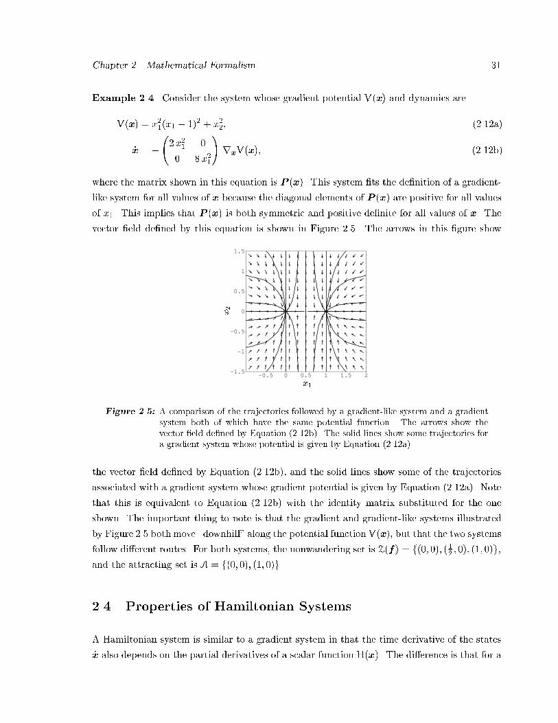
Chapter �� Mathematical Formalism ��
Example ���� Consider the system whose gradient potential V�x� and dynamics are
V�x� � x���x� � ��� � x��� �����a�
�x � ���x�� �
� �x��
�rxV�x�� �����b�
where the matrix shown in this equation is P �x�� This system �ts the de�nition of a gradient�
like system for all values of x because the diagonal elements of P �x� are positive for all values
of x�� This implies that P �x� is both symmetric and positive de�nite for all values of x� The
vector �eld de�ned by this equation is shown in Figure ���� The arrows in this �gure show
-0.5 0 0.5 1 1.5 2-1.5
-1
-0.5
0
0.5
1
1.5
x�
x�
Figure ���� A comparison of the trajectories followed by a gradient�like system and a gradientsystem both of which have the same potential function� The arrows show thevector �eld de�ned by Equation ��� �b�� The solid lines show some trajectories fora gradient system whose potential is given by Equation ��� �a��
the vector �eld de�ned by Equation �����b�� and the solid lines show some of the trajectories
associated with a gradient system whose gradient potential is given by Equation �����a�� Note
that this is equivalent to Equation �����b� with the identity matrix substituted for the one
shown� The important thing to note is that the gradient and gradient�like systems illustrated
by Figure ��� both move �downhill along the potential function V�x�� but that the two systems
follow di�erent routes� For both systems� the nonwandering set is Z�f� � f��� ��� ��� � ��� ��� ��g�and the attracting set is A � f��� ��� ��� ��g�
��� Properties of Hamiltonian Systems
A Hamiltonian system is similar to a gradient system in that the time derivative of the states
�x also depends on the partial derivatives of a scalar function H�x�� The di�erence is that for a
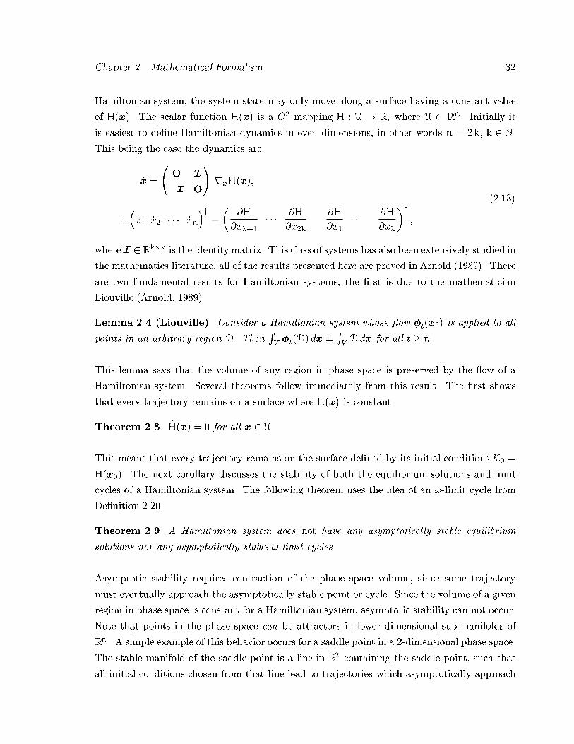
Chapter �� Mathematical Formalism ��
Hamiltonian system� the system state may only move along a surface having a constant value
of H�x�� The scalar function H�x� is a C� mapping H � U � R� where U Rn � Initially it
is easiest to de�ne Hamiltonian dynamics in even dimensions� in other words n � �k� k � N�This being the case the dynamics are
�x �
�O I
�I O
�rxH�x��
�
��x� �x� � � � �xn
y�
��H
�xk��� � � �H
�x�k� �H
�x�� � � � �H
�xk
�y�
������
where I � Rk�k is the identity matrix� This class of systems has also been extensively studied in
the mathematics literature� all of the results presented here are proved in Arnold ������� There
are two fundamental results for Hamiltonian systems� the �rst is due to the mathematician
Liouville �Arnold� ������
Lemma ��� �Liouville � Consider a Hamiltonian system whose �ow �t�x�� is applied to all
points in an arbitrary region D� ThenRV �t�D� dx �
RV D dx for all t � t��
This lemma says that the volume of any region in phase space is preserved by the "ow of a
Hamiltonian system� Several theorems follow immediately from this result� The �rst shows
that every trajectory remains on a surface where H�x� is constant�
Theorem ���� �H�x� � � for all x � U�
This means that every trajectory remains on the surface de�ned by its initial conditions K� �
H�x��� The next corollary discusses the stability of both the equilibrium solutions and limit
cycles of a Hamiltonian system� The following theorem uses the idea of an ��limit cycle from
De�nition �����
Theorem ���� A Hamiltonian system does not have any asymptotically stable equilibrium
solutions nor any asymptotically stable ��limit cycles�
Asymptotic stability requires contraction of the phase space volume� since some trajectory
must eventually approach the asymptotically stable point or cycle� Since the volume of a given
region in phase space is constant for a Hamiltonian system� asymptotic stability can not occur�
Note that points in the phase space can be attractors in lower dimensional sub�manifolds of
Rn � A simple example of this behavior occurs for a saddle point in a ��dimensional phase space�
The stable manifold of the saddle point is a line in R� containing the saddle point� such that
all initial conditions chosen from that line lead to trajectories which asymptotically approach
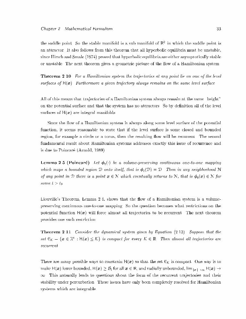
Chapter �� Mathematical Formalism ��
the saddle point� So the stable manifold is a sub�manifold of R� in which the saddle point is
an attractor� It also follows from this theorem that all hyperbolic equilibria must be unstable�
since Hirsch and Smale ������ proved that hyperbolic equilibria are either asymptotically stable
or unstable� The next theorem gives a geometric picture of the "ow of a Hamiltonian system�
Theorem ���� For a Hamiltonian system the trajectories at any point lie on one of the level
surfaces of H�x�� Furthermore a given trajectory always remains on the same level surface�
All of this means that trajectories of a Hamiltonian system always remain at the same �height
on the potential surface and that the system has no attractors� So by de�nition all of the level
surfaces of H�x� are integral manifolds�
Since the "ow of a Hamiltonian system is always along some level surface of the potential
function� it seems reasonable to state that if the level surface is some closed and bounded
region� for example a circle or a torus� then the resulting "ow will be recurrent� The second
fundamental result about Hamiltonian systems addresses exactly this issue of recurrence and
is due to Poincar�e �Arnold� ������
Lemma ��� �Poincar�e � Let �t��� be a volume�preserving continuous one�to�one mapping
which maps a bounded region D onto itself� that is �t�D� � D� Then in any neighborhood N
of any point in D there is a point x � N which eventually returns to N� that is �t�x� � N for
some t � t��
Liouvilles Theorem� Lemma ���� shows that the "ow of a Hamiltonian system is a volume�
preserving continuous one�to�one mapping� So the question becomes what restrictions on the
potential function H�x� will force almost all trajectories to be recurrent� The next theorem
provides one such restriction�
Theorem ����� Consider the dynamical system given by Equation ������� Suppose that the
set CK � fx � Rn � H�x� � Kg is compact for every K � R� Then almost all trajectories are
recurrent�
There are many possible ways to constrain H�x� so that the set CK is compact� One way is to
make H�x� lower bounded� H�x� � Bl for all x � R� and radially unbounded� limkxk��H�x���� This naturally leads to questions about the form of the recurrent trajectories and their
stability under perturbation� These issues have only been completely resolved for Hamiltonian
systems which are integrable�
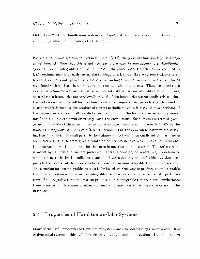
Chapter �� Mathematical Formalism ��
Denition ����� A Hamiltonian system is integrable if there exist k scalar functions Ii�x��
i � �� � � � �k which are �rst integrals of the system�
For the autonomous systems de�ned in Equation ������� the potential function H�x� is always
a �rst integral� Note that this is not necessarily the case for non�autonomous Hamiltonian
systems� For an integrable Hamiltonian system� the phase space trajectories are con�ned to
k�dimensional manifolds each having the topology of a k�torus� So the system trajectories all
have the form of windings around these tori� A winding around a torus will have k frequencies
associated with it� since there are k circles associated with any k�torus� These frequencies are
said to be rationally related if all pairwise quotients of the frequencies yield rational numbers�
otherwise the frequencies are irrationally related� If the frequencies are rationally related� then
the motion on the torus will form a closed orbit which repeats itself periodically� Because this
closed orbit is formed by the product of several periodic motions� it is called multi�periodic� If
the frequencies are irrationally related then the motion on the torus will never exactly repeat
itself and a single orbit will eventually cover the entire torus� Such orbits are termed quasi�
periodic� The fate of these tori under perturbation was illuminated in the early ����s by the
famous Kolmogorov Arnold Moser �KAM� Theorem� This theorem can be paraphrased as say�
ing that for su�ciently small perturbations almost all tori with irrationally related frequencies
are preserved� The theorem gives a condition on the frequencies which shows how irrational
the relationship must be in order for the torus in question to be preserved� This de�nes what
is meant by �almost all tori are preserved� There is however� no general way to determine
whether a perturbation is �su�ciently small� It turns out that the tori which are destroyed
provide the �seeds of the chaotic behavior observed in non�integrable Hamiltonian systems�
The situation for non�integrable systems is far less clear� One way to produce a non�integrable
Hamiltonian system is to perturb an integrable one� It is not known whether �small perturba�
tions of all integrable Hamiltonians can produce all non�integrable Hamiltonians� Furthermore
there is no test to determine whether a given Hamiltonian system is integrable or not in the
�rst place�
��� Properties of Hamiltonian�Like Systems
Many of the useful properties of Hamiltonian systems are also possessed by a more general class
of dynamical systems� which will be referred to as Hamiltonian�like systems� Hamiltonian�like
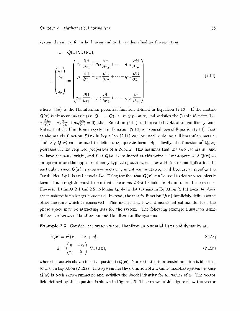
Chapter �� Mathematical Formalism ��
system dynamics� for n both even and odd� are described by the equation
�x � Q�x�rxH�x��
�
BBBBB�
�x�
�x����
�xn
�CCCCCA �
BBBBBBBBBBB�
q���H
�x�� q��
�H
�x�� � � � � q�n
�H
�xn
q���H
�x�� q��
�H
�x�� � � � � q�n
�H
�xn���
qn��H
�x�� qn�
�H
�x�� � � �� qnn
�H
�xn
�CCCCCCCCCCCA�
������
where H�x� is the Hamiltonian potential function de�ned in Equation ������� If the matrix
Q�x� is skew�symmetric �i�e� Qy � �Q� at every point x� and satis�es the Jacobi identity �i�e�
qli�qjk�xl
� qlj�qki�xl
� qlk�qij�xl
� ��� then Equation ������ will be called a Hamiltonian�like system�
Notice that the Hamiltonian system in Equation ������ is a special case of Equation ������� Just
as the matrix function P �x� in Equation ������ can be used to de�ne a Riemannian metric�
similarly Q�x� can be used to de�ne a symplectic form� Speci�cally� the function xy�Q� x�
possesses all the required properties of a ��form� This assumes that the two vectors x� and
x� have the same origin� and that Q�x� is evaluated at this point� The properties of Q�x� as
an operator are the opposite of many typical operators� such as addition or multiplication� In
particular� since Q�x� is skew�symmetric it is anti�commutative� and because it satis�es the
Jacobi identity it is anti�associative� Using the fact thatQ�x� can be used to de�ne a symplectic
form� it is straightforward to see that Theorems ��� ���� hold for Hamiltonian�like systems�
However� Lemmas ��� and ��� no longer apply to the systems in Equation ������ because phase
space volume is no longer conserved� Instead� the matrix function Q�x� implicitly de�nes some
other measure which is conserved� This means that lower dimensional submanifolds of the
phase space may be attracting sets for the system� The following example illustrates some
di�erences between Hamiltonian and Hamiltonian�like systems�
Example ���� Consider the system whose Hamiltonian potential H�x� and dynamics are
H�x� � x���x� � ��� � x��� �����a�
�x �
�� �x�x� �
�rxH�x�� �����b�
where the matrix shown in this equation isQ�x�� Notice that this potential function is identical
to that in Equation �����a�� This system �ts the de�nition of a Hamiltonian�like system because
Q�x� is both skew�symmetric and satis�es the Jacobi identity for all values of x� The vector
�eld de�ned by this equation is shown in Figure ���� The arrows in this �gure show the vector
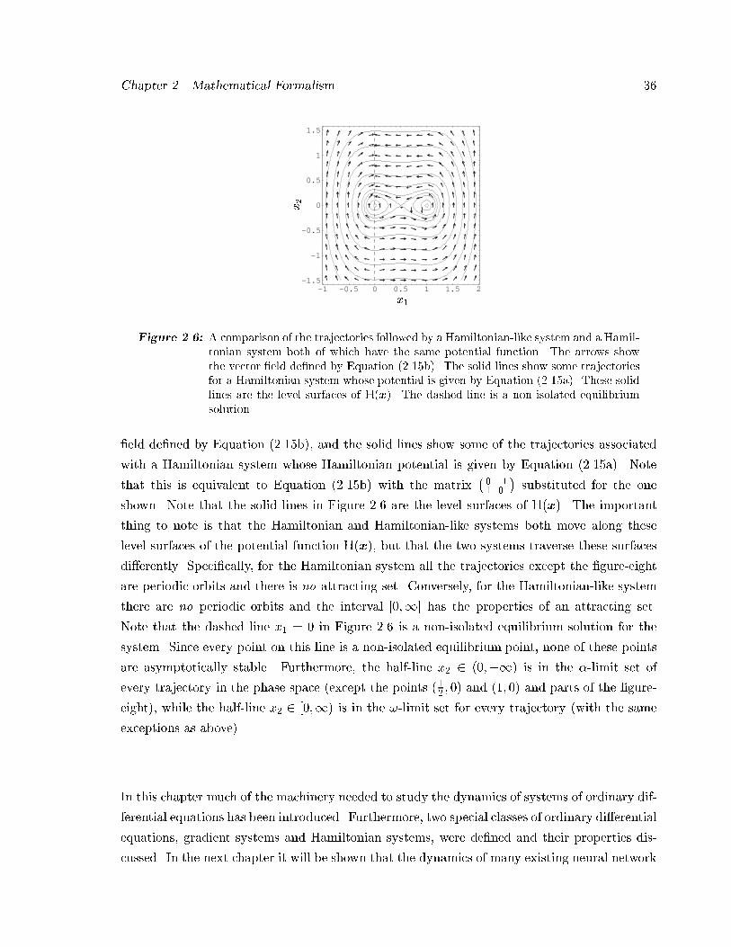
Chapter �� Mathematical Formalism ��
-1 -0.5 0 0.5 1 1.5 2-1.5
-1
-0.5
0
0.5
1
1.5
x�
x�
Figure ���� A comparison of the trajectories followed by a Hamiltonian�like system and a Hamil�tonian system both of which have the same potential function� The arrows showthe vector �eld de�ned by Equation ��� �b�� The solid lines show some trajectoriesfor a Hamiltonian system whose potential is given by Equation ��� �a�� These solidlines are the level surfaces of H�x�� The dashed line is a non�isolated equilibriumsolution�
�eld de�ned by Equation �����b�� and the solid lines show some of the trajectories associated
with a Hamiltonian system whose Hamiltonian potential is given by Equation �����a�� Note
that this is equivalent to Equation �����b� with the matrix�� ��� �
�substituted for the one
shown� Note that the solid lines in Figure ��� are the level surfaces of H�x�� The important
thing to note is that the Hamiltonian and Hamiltonian�like systems both move along these
level surfaces of the potential function H�x�� but that the two systems traverse these surfaces
di�erently� Speci�cally� for the Hamiltonian system all the trajectories except the �gure�eight
are periodic orbits and there is no attracting set� Conversely� for the Hamiltonian�like system
there are no periodic orbits and the interval ����� has the properties of an attracting set�
Note that the dashed line x� � � in Figure ��� is a non�isolated equilibrium solution for the
system� Since every point on this line is a non�isolated equilibrium point� none of these points
are asymptotically stable� Furthermore� the half�line x� � ������ is in the ��limit set of
every trajectory in the phase space �except the points ��� � �� and ��� �� and parts of the �gure�
eight�� while the half�line x� � ����� is in the ��limit set for every trajectory �with the same
exceptions as above��
In this chapter much of the machinery needed to study the dynamics of systems of ordinary dif�
ferential equations has been introduced� Furthermore� two special classes of ordinary di�erential
equations� gradient systems and Hamiltonian systems� were de�ned and their properties dis�
cussed� In the next chapter it will be shown that the dynamics of many existing neural network

Chapter �� Mathematical Formalism ��
architectures can be decomposed into the sum of a gradient�like term and a Hamiltonian�like
term� This result will then be used to analyze the dynamics of such systems�
Chapter �
Gradient�Hamiltonian Analysis
One way to make use of gradient and Hamiltonian systems is to decompose an existing system
into a gradient portion and a Hamiltonian portion� The central idea of this chapter is to
show that many neural network models from the literature can be decomposed into the sum
of a gradient�like system and a Hamiltonian�like system� In Section ���� the results of Cohen
and Grossberg ������ for fully connected networks� with a symmetric constant connection �i�e�
weight� matrix� are reviewed� Then in Section ���� it is shown that such networks can be written
as gradient�like systems� This result is extended in Section ��� to show that fully connected
networks with certain types of weight dynamics are also gradient�like systems� It is shown
that networks with Hebbian weight update� anti�Hebbian weight update� di�erential Hebbian
weight update� and higher�order Hebbian weight update are special cases of this result� It is also
demonstrated that networks which are not fully connected� such as certain forms of multilayer
networks� are gradient�like systems� Some example simulations of a neural network with simple
gradient�like dynamics are performed in Section ���� Up to that point all the systems under
consideration have only a gradient�like character� In Section ���� the results of Mendes and
Duarte ������ for fully connected networks with an arbitrary constant connection matrix are
reviewed� That paper shows that such networks can be formulated as the sum of a gradient�like
system and a Hamiltonian�like system� Then in Section ���� that result is extended to networks
with both Hebbian and gated weight update� It is also shown that feedforward networks can
be written in this form� In Section ��� several existing recurrent neural network architectures
are examined in the context of this gradient�Hamiltonian decomposition� Lastly� Section ���
is an assessment of the utility of the gradient�Hamiltonian decomposition for neural network
analysis�
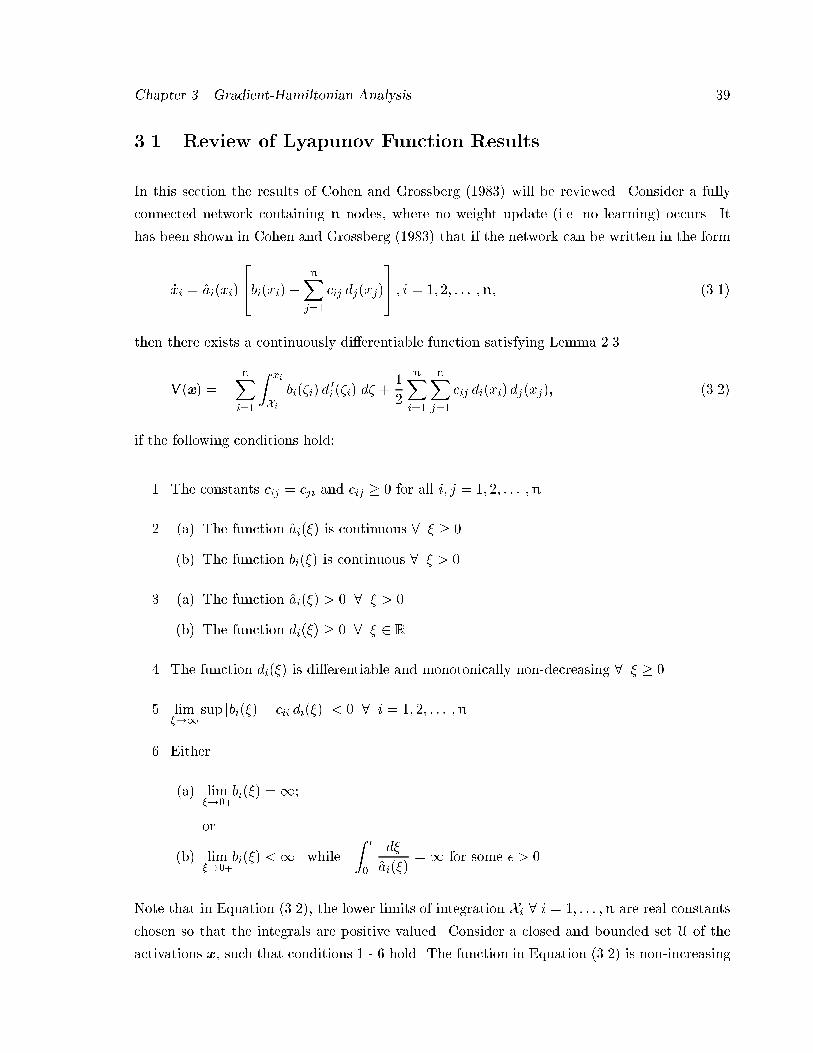
Chapter �� Gradient�Hamiltonian Analysis ��
��� Review of Lyapunov Function Results
In this section the results of Cohen and Grossberg ������ will be reviewed� Consider a fully
connected network containing n nodes� where no weight update �i�e� no learning� occurs� It
has been shown in Cohen and Grossberg ������ that if the network can be written in the form
�xi � ai�xi�
�bi�xi�� nX
j��
cij dj�xj�
�� � i � �� �� � � � �n� �����
then there exists a continuously di�erentiable function satisfying Lemma ���
V�x� � �nXi��
Z xi
Xibi��i� d
�i ��i� d� �
�
�
nXi��
nXj��
cij di�xi� dj�xj�� �����
if the following conditions hold�
�� The constants cij � cji and cij � � for all i� j � �� �� � � � �n�
�� �a� The function ai��� is continuous � � � ��
�b� The function bi��� is continuous � � � ��
�� �a� The function ai��� � � � � � ��
�b� The function di��� � � � � � R�
�� The function di��� is di�erentiable and monotonically non�decreasing � � � ��
�� lim���
sup �bi���� cii di���� � � � i � �� �� � � � �n�
�� Either
�a� lim����
bi��� ���
or
�b� lim����
bi��� �� while
Z �
�
d�
ai����� for some � ��
Note that in Equation ������ the lower limits of integration Xi � i � �� � � � �n are real constants
chosen so that the integrals are positive valued� Consider a closed and bounded set U of the
activations x� such that conditions � � � hold� The function in Equation ����� is non�increasing
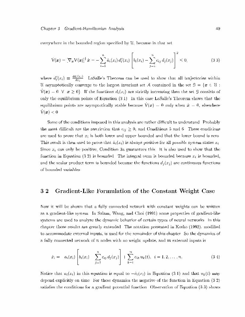
Chapter �� Gradient�Hamiltonian Analysis ��
everywhere in the bounded region speci�ed by U� because in that set
�V�x� � �rxV�x��y �x � �nXi��
ai�xi� d�i �xi�
�bi�xi�� nX
j��
cij dj�xj�
���
� �� �����
where d �i �xi� � ddi�xidxi
� LaSalles Theorem can be used to show that all trajectories within
U asymptotically converge to the largest invariant set A contained in the set G � fx � U �
�V�x� � � � x � �g� If the functions di�xi� are strictly increasing then the set G consists of
only the equilibrium points of Equation ������ In this case LaSalles Theorem shows that the
equilibrium points are asymptotically stable because �V�x� � � only when �x � �� elsewhere
�V�x� � ��
Some of the conditions imposed in this analysis are rather di�cult to understand� Probably
the most di�cult are the restriction that cij � �� and Conditions � and �� These conditions
are used to prove that xi is both lower and upper bounded and that the lower bound is zero�
This result is then used to prove that ai�xi� is always positive for all possible system states xi�
Since xi can only be positive� Condition �a guarantees this� It is also used to show that the
function in Equation ����� is bounded� The integral term is bounded because xi is bounded�
and the scalar product term is bounded because the functions dj�xj� are continuous functions
of bounded variables�
��� Gradient�Like Formulation of the Constant Weight Case
Now it will be shown that a fully connected network with constant weights can be written
as a gradient�like system� In Salam� Wang� and Choi ������ some properties of gradient�like
systems are used to analyze the dynamic behavior of certain types of neural networks� In this
chapter those results are greatly extended� The notation presented in Kosko ������� modi�ed
to accommodate external inputs� is used for the remainder of this chapter� So the dynamics of
a fully connected network of n nodes with no weight update� and m external inputs is
�xi � �ai�xi� �bi�xi�� nX
j��
cij dj�xj�
���
mXk��
eik uk�t�� i � �� �� � � � �n� �����
Notice that ai�xi� in this equation is equal to � ai�xi� in Equation ����� and that uk�t� may
depend explicitly on time� For these dynamics the negative of the function in Equation �����
satis�es the conditions for a gradient potential function� Observation of Equation ����� shows
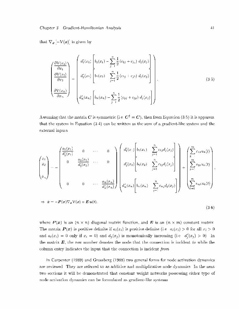
Chapter �� Gradient�Hamiltonian Analysis ��
that rx ��V�x�� is given by
�BBBBBBBBB�
�V�x��
�x�
�V�x��
�x����
�V�xn�
�xn
�CCCCCCCCCA
�BBBBBBBBBBBBBBB�
d ���x��
��b��x���
nXj��
��c�j � cj�� dj�xj�
��
d ���x��
��b��x���
nXj��
��c�j � cj�� dj�xj�
��
���
d �n�xn�
��bn�xn��
nXj��
��cpj � cjp� dj�xj�
��
�CCCCCCCCCCCCCCCA
� �����
Assuming that the matrixC is symmetric �i�e�Cy � C�� then from Equation ����� it is apparent
that the system in Equation ����� can be written as the sum of a gradient�like system and the
external inputs
�BBBB�
�x��x����
�xn
�CCCCA �
�BBBBBBBBBBBB�
a��x��
d ���x��� � � � �
�a��x��
d ���x��� � � �
������
� � ����
� � � � �an�xn�
d �n�xn�
�CCCCCCCCCCCCA
�BBBBBBBBBBBBBBB�
d ���x��
��b��x���
nXj��
c�jdj�xj�
��
d ���x��
��b��x���
nXj��
c�jdj�xj�
��
���
d �n�xn�
��bn�xn��
nXj��
cnjdj�xj�
��
�CCCCCCCCCCCCCCCA
�
�BBBBBBBBBBBB�
mXk��
e�kuk�t�
mXk��
e�kuk�t�
���mXk��
enkuk�t�
�CCCCCCCCCCCCA�
� �x �P �x�rxV�x� �E u�t��
�����
where P �x� is an �n n� diagonal matrix function� and E is an �n m� constant matrix�
The matrix P �x� is positive de�nite if ai�xi� is positive de�nite �i�e� ai�xi� � � for all xi � �
and ai�xi� � � only if xi � �� and dj�xj� is monotonically increasing �i�e� d �j�xj� � ��� In
the matrix E� the row number denotes the node that the connection is incident to while the
column entry indicates the input that the connection is incident from�
In Carpenter ������ and Grossberg ������ two general forms for node activation dynamics
are reviewed� They are referred to as additive and multiplicative node dynamics� In the next
two sections it will be demonstrated that constant weight networks possessing either type of
node activation dynamics can be formulated as gradient�like systems�
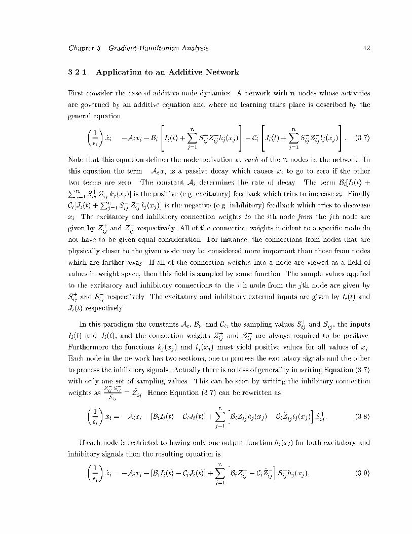
Chapter �� Gradient�Hamiltonian Analysis ��
����� Application to an Additive Network
First consider the case of additive node dynamics� A network with n nodes whose activities
are governed by an additive equation and where no learning takes place is described by the
general equation
��
i
��xi � �Aixi � Bi
�Ii�t� � nX
j��
S�ijZ
�ijkj�xj�
��� Ci
�Ji�t� � nX
j��
S�ijZ�ij lj�xj�
�� � �����
Note that this equation de�nes the node activation at each of the n nodes in the network� In
this equation the term �Ai xi is a passive decay which causes xi to go to zero if the other
two terms are zero� The constant Ai determines the rate of decay� The term Bi�Ii�t� �Pnj�� S
�ij Z
�ij kj�xj�� is the positive �e�g� excitatory� feedback which tries to increase xi� Finally
Ci�Ji�t� �Pn
j�� S�ij Z
�ij lj�xj�� is the negative �e�g� inhibitory� feedback which tries to decrease
xi� The excitatory and inhibitory connection weights to the ith node from the jth node are
given by Z�ij and Z�
ij respectively� All of the connection weights incident to a speci�c node do
not have to be given equal consideration� For instance� the connections from nodes that are
physically closer to the given node may be considered more important than those from nodes
which are farther away� If all of the connection weights into a node are viewed as a �eld of
values in weight space� then this �eld is sampled by some function� The sample values applied
to the excitatory and inhibitory connections to the ith node from the jth node are given by
S�ij and S�ij respectively� The excitatory and inhibitory external inputs are given by Ii�t� and
Ji�t� respectively�
In this paradigm the constants Ai� Bi� and Ci� the sampling values S�ij and S�ij � the inputs
Ii�t� and Ji�t�� and the connection weights Z�ij and Z�
ij are always required to be positive�
Furthermore the functions kj�xj� and lj�xj� must yield positive values for all values of xj �
Each node in the network has two sections� one to process the excitatory signals and the other
to process the inhibitory signals� Actually there is no loss of generality in writing Equation �����
with only one set of sampling values� This can be seen by writing the inhibitory connection
weights asZ�ij S
�ij
S�ij� %Z�
ij � Hence Equation ����� can be rewritten as
��
i
��xi � �Aixi � �BiIi�t�� CiJi�t�� �
nXj��
hBiZ�
ijkj�xj�� Ci %Z�ij lj�xj�
iS�ij � �����
If each node is restricted to having only one output function hi�xi� for both excitatory and
inhibitory signals then the resulting equation is��
i
��xi � �Aixi � �BiIi�t�� CiJi�t�� �
nXj��
hBiZ�
ij � Ci %Z�ij
iS�ijhj�xj�� �����
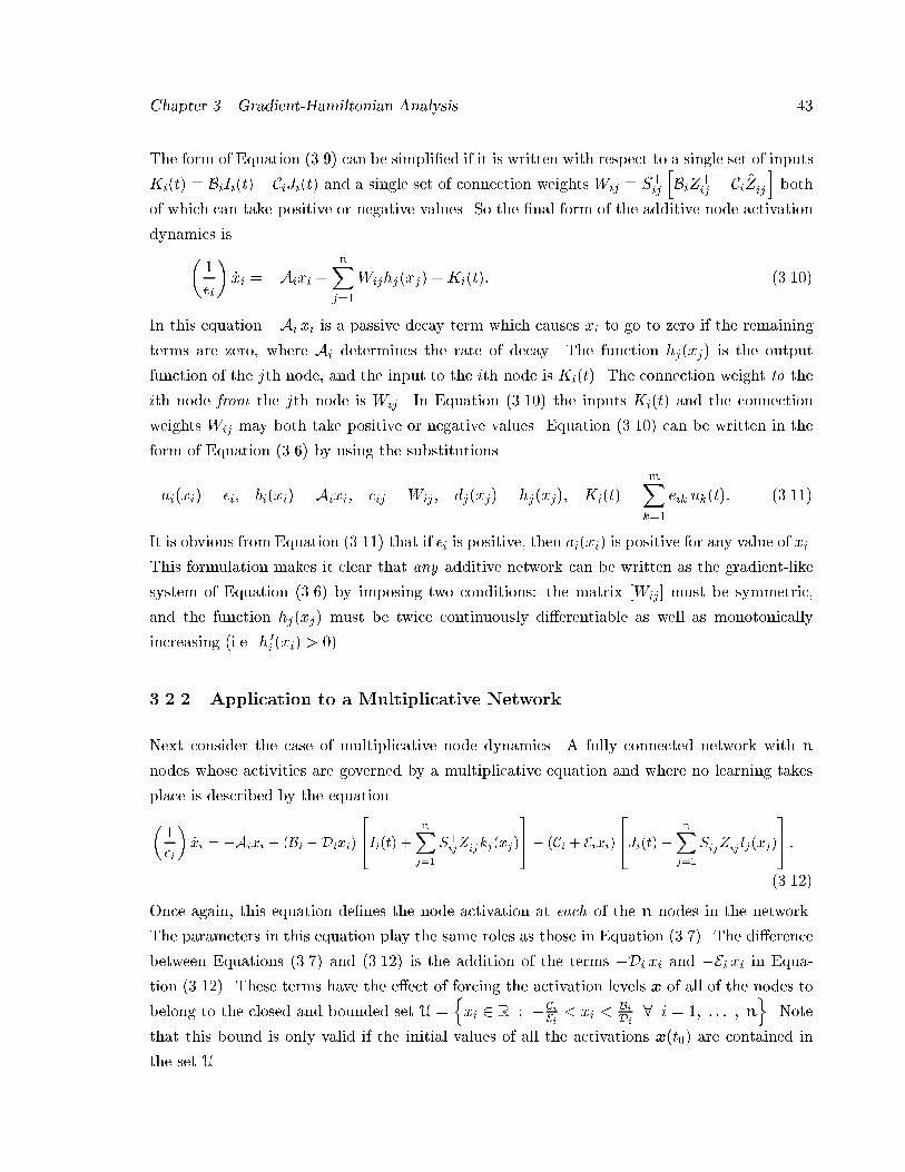
Chapter �� Gradient�Hamiltonian Analysis ��
The form of Equation ����� can be simpli�ed if it is written with respect to a single set of inputs
Ki�t� � BiIi�t�� CiJi�t� and a single set of connection weights Wij � S�ij
hBiZ�
ij � Ci %Z�ij
iboth
of which can take positive or negative values� So the �nal form of the additive node activation
dynamics is��
i
��xi � �Aixi �
nXj��
Wijhj�xj� �Ki�t�� ������
In this equation �Ai xi is a passive decay term which causes xi to go to zero if the remaining
terms are zero� where Ai determines the rate of decay� The function hj�xj� is the output
function of the jth node� and the input to the ith node is Ki�t�� The connection weight to the
ith node from the jth node is Wij� In Equation ������ the inputs Ki�t� and the connection
weights Wij may both take positive or negative values� Equation ������ can be written in the
form of Equation ����� by using the substitutions
ai�xi� � i� bi�xi� � Aixi� cij � Wij� dj�xj� � hj�xj�� Ki�t� �mXk��
eik uk�t�� ������
It is obvious from Equation ������ that if i is positive� then ai�xi� is positive for any value of xi�
This formulation makes it clear that any additive network can be written as the gradient�like
system of Equation ����� by imposing two conditions� the matrix �Wij� must be symmetric�
and the function hj�xj� must be twice continuously di�erentiable as well as monotonically
increasing �i�e� h �i �xi� � ���
����� Application to a Multiplicative Network
Next consider the case of multiplicative node dynamics� A fully connected network with n
nodes whose activities are governed by a multiplicative equation and where no learning takes
place is described by the equation
�
�i
�xi �Aixi � �Bi �Dixi�
��Ii�t� �
nXj��
S�ijZ
�ijkj�xj�
��� �Ci � Eixi�
��Ji�t� �
nXj��
S�ijZ�ij lj�xj�
�� �������
Once again� this equation de�nes the node activation at each of the n nodes in the network�
The parameters in this equation play the same roles as those in Equation ������ The di�erence
between Equations ����� and ������ is the addition of the terms �Di xi and �Ei xi in Equa�
tion ������� These terms have the e�ect of forcing the activation levels x of all of the nodes to
belong to the closed and bounded set U �nxi � R � �Ci
Ei � xi �BiDi
� i � �� � � � � no� Note
that this bound is only valid if the initial values of all the activations x�t�� are contained in
the set U�
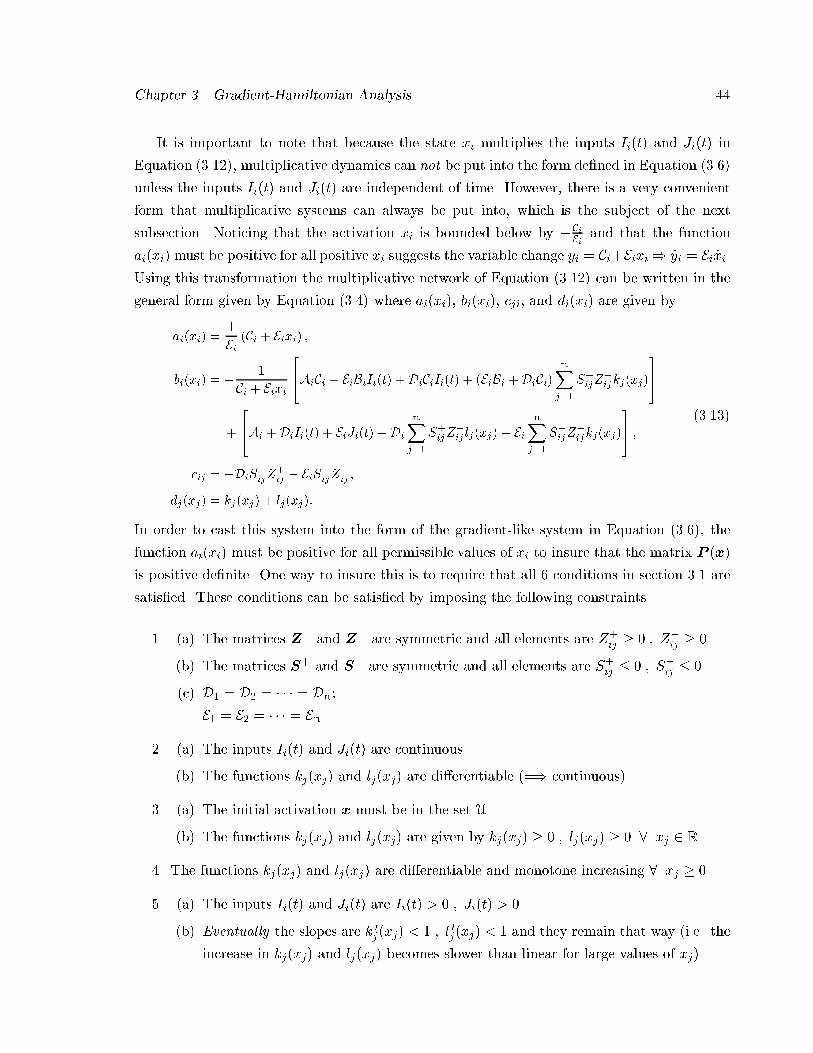
Chapter �� Gradient�Hamiltonian Analysis ��
It is important to note that because the state xi multiplies the inputs Ii�t� and Ji�t� in
Equation ������� multiplicative dynamics can not be put into the form de�ned in Equation �����
unless the inputs Ii�t� and Ji�t� are independent of time� However� there is a very convenient
form that multiplicative systems can always be put into� which is the subject of the next
subsection� Noticing that the activation xi is bounded below by �CiEi and that the function
ai�xi� must be positive for all positive xi suggests the variable change yi � Ci�Eixi � �yi � Ei �xi�Using this transformation the multiplicative network of Equation ������ can be written in the
general form given by Equation ����� where ai�xi�� bi�xi�� cji� and di�xi� are given by
ai�xi�
Ei�Ci � Eixi� �
bi�xi� �
Ci � Eixi
��AiCi � EiBiIi�t� �DiCiIi�t� � �EiBi �DiCi�
nXj��
S�ijZ
�ijkj�xj�
��
�
��Ai �DiIi�t� � EiJi�t��Di
nXj��
S�ijZ
�ij lj�xj�� Ei
nXj��
S�ijZ�ijkj�xj�
�� �
cij �DiS�ijZ
�ij � EiS
�ijZ
�ij �
dj�xj� kj�xj� � lj�xj��
������
In order to cast this system into the form of the gradient�like system in Equation ������ the
function ai�xi� must be positive for all permissible values of xi to insure that the matrix P �x�
is positive de�nite� One way to insure this is to require that all � conditions in section ��� are
satis�ed� These conditions can be satis�ed by imposing the following constraints�
�� �a� The matrices Z� and Z� are symmetric and all elements are Z�ij � � � Z�
ij � ��
�b� The matrices S� and S� are symmetric and all elements are S�ij � � � S�ij � ��
�c� D� � D� � � � � � Dn�E� � E� � � � � � En�
�� �a� The inputs Ii�t� and Ji�t� are continuous�
�b� The functions kj�xj� and lj�xj� are di�erentiable ��� continuous��
�� �a� The initial activation x must be in the set U�
�b� The functions kj�xj� and lj�xj� are given by kj�xj� � � � lj�xj� � � � xj � R�
�� The functions kj�xj� and lj�xj� are di�erentiable and monotone increasing � xj � ��
�� �a� The inputs Ii�t� and Ji�t� are Ii�t� � � � Ji�t� � ��
�b� Eventually the slopes are k �j�xj� � � � l �j�xj� � � and they remain that way �i�e� the
increase in kj�xj� and lj�xj� becomes slower than linear for large values of xj��
Chapter �� Gradient�Hamiltonian Analysis ��
�� �a� If the functions kj�xj� and lj�xj� do not go to zero as xj goes to zero or if they go
to zero slower than linearly� then �a� holds�
�b� If the functions kj�xj� and lj�xj� go to zero faster than linearly then �b� holds�
Notice that Condition � is true no matter how the functions kj�xj� and lj�xj� are selected� The
restrictions on Di and Ei in Condition � can be explained intuitively in the following way� The
activation xi of the ith node is upper and lower bounded by BiDi
and �CiEi respectively� The time
constants� which determine the speed at which xi approaches these upper and lower bounds�
are given by �Di
and �Ei respectively� Hence Condition � states that the rate� at which a node
approaches the upper or lower bound of its activation� is identical for all nodes in the network�
Notice that the rate at which the upper and lower bounds are approached may be di�erent�
Also each node may have a di�erent upper and lower activation bound� since Bi and Ci may
be set di�erently for every node� The restriction imposed on the slopes of kj�xj� and lj�xj� by
Condition � can not be removed if the system described by Equation ������ is to be a stable
system� However� given the computational advantages of choosing a sigmoidal output function
proven in Grossberg ������� this hardly seems a serious limitation�
����� A Control Theory Viewpoint
It is instructive to look at the additive and multiplicative systems de�ned in the two previous
subsections from the viewpoint of control theory� Since the additive dynamics in Equation �����
are merely a special case of the multiplicative dynamics in Equation ������� only the proper�
ties of the multiplicative system will be discussed� A diagram of Equation ������ appears in
Figure ���� This �gure makes it clear that a multiplicative system is a bilinear system with
a speci�c type of nonlinear state feedback� The input u�t� is a �n element vector consisting
of u�t� ��I�t���J�t
�� The matrix A is an �n n� diagonal matrix with the terms �Ai along
the diagonal� The matrix B is �n �n� matrix given by B � �B��� C�� where B and C are
�n n� diagonal matrices having the terms Bi and �Ci respectively along the diagonal� The
matrices Dk where k � �� �� � � � � �n are also �n n� and diagonal� Speci�cally� the matrix
Dk for k � �� �� � � � �n has the term �Dk at the kth position on the diagonal� and has � for
all other entries� When k � n � ��n � �� � � � � �n� Dk has the term �Ek�n at the kth po�
sition on the diagonal� and � everywhere else� The matrix Z is a ��n �n� matrix given
by Z ��S�Z�
��� O��� ��� ��� ���S�Z�
��� O
�� where the operation � denotes the Schur product which is de�ned in
Kailath ������ as �A � B�ij � aijbij� Lastly� the vector function f��� returns a �n element
vector of the form f�x� ��k�x������l�x
�� So this is a �n�input n�output system� where the inputs
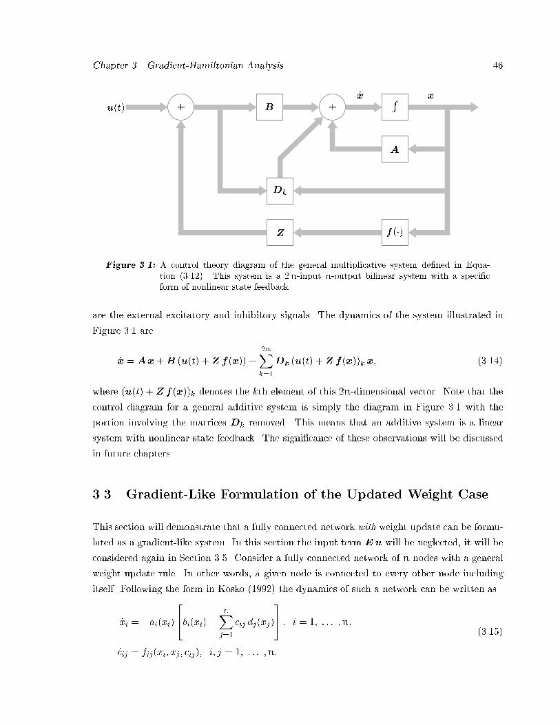
Chapter �� Gradient�Hamiltonian Analysis ��
A
RB
Dk
Z f���
u�t��x x
��
Figure ���� A control theory diagram of the general multiplicative system de�ned in Equa�tion ��� ��� This system is a �n�input n�output bilinear system with a speci�cform of nonlinear state feedback�
are the external excitatory and inhibitory signals� The dynamics of the system illustrated in
Figure ��� are
�x � Ax�B �u�t� �Z f�x�� �
�nXk��
Dk �u�t� �Z f�x��k x� ������
where �u�t� �Z f�x��k denotes the kth element of this �n�dimensional vector� Note that the
control diagram for a general additive system is simply the diagram in Figure ��� with the
portion involving the matrices Dk removed� This means that an additive system is a linear
system with nonlinear state feedback� The signi�cance of these observations will be discussed
in future chapters�
��� Gradient�Like Formulation of the Updated Weight Case
This section will demonstrate that a fully connected network with weight update can be formu�
lated as a gradient�like system� In this section the input term Eu will be neglected� it will be
considered again in Section ���� Consider a fully connected network of n nodes with a general
weight update rule� In other words� a given node is connected to every other node including
itself� Following the form in Kosko ������ the dynamics of such a network can be written as
�xi � �ai�xi� �bi�xi�� nX
j��
cij dj�xj�
�� � i � �� � � � �n�
�cij � fij�xi� xj � cij�� i� j � �� � � � �n�
������
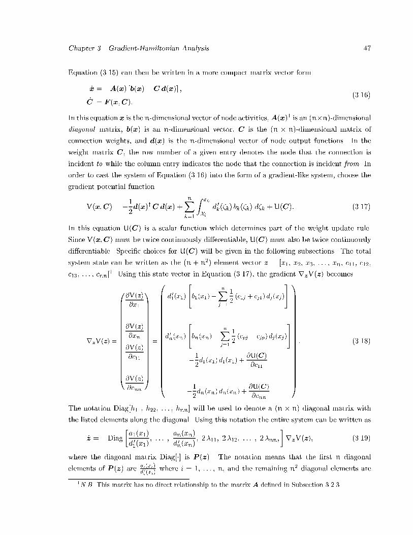
Chapter �� Gradient�Hamiltonian Analysis ��
Equation ������ can then be written in a more compact matrix�vector form
�x � �A�x� �b�x��C d�x�� ��C � F �x�C��
������
In this equation x is the n�dimensional vector of node activities�A�x�� is an �n n��dimensional
diagonal matrix� b�x� is an n�dimensional vector� C is the �n n��dimensional matrix of
connection weights� and d�x� is the n�dimensional vector of node output functions� In the
weight matrix C� the row number of a given entry denotes the node that the connection is
incident to while the column entry indicates the node that the connection is incident from� In
order to cast the system of Equation ������ into the form of a gradient�like system� choose the
gradient potential function
V�x�C� � ��
�d�x�yC d�x� �
nXk��
Z xk
Xid �k��k� bk��k� d�k �U�C�� ������
In this equation U�C� is a scalar function which determines part of the weight update rule�
Since V�x�C� must be twice continuously di�erentiable� U�C� must also be twice continuously
di�erentiable� Speci�c choices for U�C� will be given in the following subsections� The total
system state can be written as the �n � n�� element vector z � �x�� x�� x�� � � � � xn� c��� c���
c��� � � � � cnn�y� Using this state vector in Equation ������� the gradient rzV�z� becomes
rzV�z�
�BBBBBBBBBBBBBBBBBB�
�V�z�
�x����
�V�z�
�xn
�V�z�
�c�����
�V�z�
�cnn
�CCCCCCCCCCCCCCCCCCA
�BBBBBBBBBBBBBBBBBBBBBB�
d ���x��
��b��x���
nXj��
��c�j � cj�� dj�xj�
��
���
d �n�xn�
��bn�xn��
nXj��
��cpj � cjp� dj�xj�
��
�
�d��x�� d��x�� �
�U�C�
�c�����
�
�dn�xn� dn�xn� �
�U�C�
�cnn
�CCCCCCCCCCCCCCCCCCCCCCA
� ������
The notation Diag�h��� h��� � � � � hnn� will be used to denote a �n n� diagonal matrix with
the listed elements along the diagonal� Using this notation the entire system can be written as
�z � �Diag
�a��x��
d ���x��� � � � �
an�xn�
d �n�xn�� ����� ����� � � � � ��nn�
�rzV�z�� ������
where the diagonal matrix Diag��� is P �z�� The notation means that the �rst n diagonal
elements of P �z� are ai�xid �i �xi
where i � �� � � � � n� and the remaining n� diagonal elements are
�N�B� This matrix has no direct relationship to the matrix A de�ned in Subsection ������
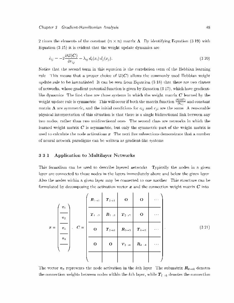
Chapter �� Gradient�Hamiltonian Analysis ��
� times the elements of the constant �n n� matrix �� By identifying Equation ������ with
Equation ������ it is evident that the weight update dynamics are
�cij � ���U�C�
�cij� �ij di�xi� dj�xj�� ������
Notice that the second term in this equation is the correlation term of the Hebbian learning
rule� This means that a proper choice of U�C� allows the commonly used Hebbian weight
update rule to be instantiated� It can be seen from Equation ������ that there are two classes
of networks� whose gradient potential function is given by Equation ������� which have gradient�
like dynamics� The �rst class are those systems in which the weight matrix C learned by the
weight update rule is symmetric� This will occur if both the matrix function �U�C�cij
and constant
matrix � are symmetric� and the initial conditions for cij and cji are the same� A reasonable
physical interpretation of this situation is that there is a single bidirectional link between any
two nodes� rather than two unidirectional ones� The second class are networks in which the
learned weight matrix C is asymmetric� but only the symmetric part of the weight matrix is
used to calculate the node activations x� The next �ve subsections demonstrate that a number
of neural network paradigms can be written as gradient�like systems�
����� Application to Multilayer Networks
This formalism can be used to describe layered networks� Typically the nodes in a given
layer are connected to those nodes in the layers immediately above and below the given layer�
Also the nodes within a given layer may be connected to one another� This structure can be
formulated by decomposing the activation vector x and the connection weight matrix C into
x
�BBBBBBBBBBBBBBB�
v�
v�
v�
v�
���
�CCCCCCCCCCCCCCCA
� C
�BBBBBBBBBBBBBBBBBBBBBBBB�
R��� T ��� O O � � �
T ��� R��� T ��� O � � �
O T ��� R��� T ��� � � �
O O T ��� R��� � � �
������
������
� � �
�CCCCCCCCCCCCCCCCCCCCCCCCA
� ������
The vector vk represents the node activation in the kth layer� The submatrix Rk�k denotes
the connection weights between nodes within the kth layer� while T l�k denotes the connection
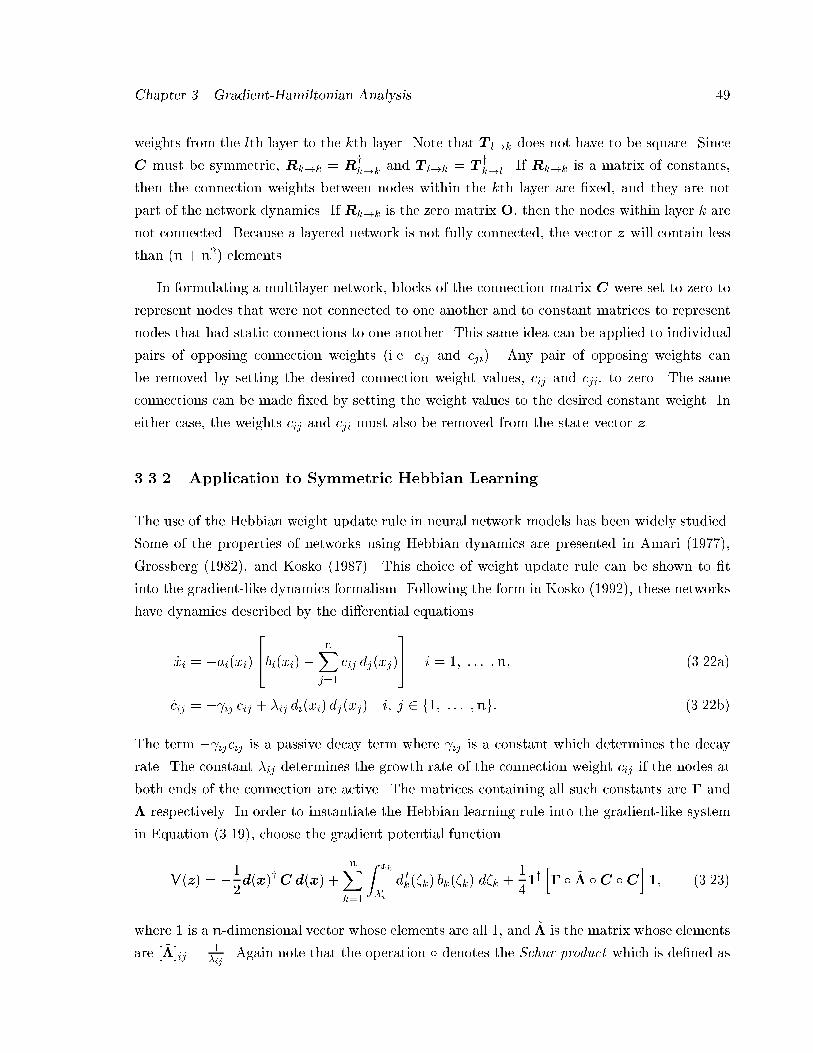
Chapter �� Gradient�Hamiltonian Analysis ��
weights from the lth layer to the kth layer� Note that T l�k does not have to be square� Since
C must be symmetric� Rk�k � Ryk�k and T l�k � T
yk�l� If Rk�k is a matrix of constants�
then the connection weights between nodes within the kth layer are �xed� and they are not
part of the network dynamics� If Rk�k is the zero matrix O� then the nodes within layer k are
not connected� Because a layered network is not fully connected� the vector z will contain less
than �n� n�� elements�
In formulating a multilayer network� blocks of the connection matrix C were set to zero to
represent nodes that were not connected to one another and to constant matrices to represent
nodes that had static connections to one another� This same idea can be applied to individual
pairs of opposing connection weights �i�e� cij and cji�� Any pair of opposing weights can
be removed by setting the desired connection weight values� cij and cji� to zero� The same
connections can be made �xed by setting the weight values to the desired constant weight� In
either case� the weights cij and cji must also be removed from the state vector z�
����� Application to Symmetric Hebbian Learning
The use of the Hebbian weight update rule in neural network models has been widely studied�
Some of the properties of networks using Hebbian dynamics are presented in Amari �������
Grossberg ������� and Kosko ������� This choice of weight update rule can be shown to �t
into the gradient�like dynamics formalism� Following the form in Kosko ������� these networks
have dynamics described by the di�erential equations
�xi � �ai�xi� �bi�xi�� nX
j��
cij dj�xj�
�� i � �� � � � �n� �����a�
�cij � ��ij cij � �ij di�xi� dj�xj� i� j � f�� � � � �ng� �����b�
The term ��ijcij is a passive decay term where �ij is a constant which determines the decay
rate� The constant �ij determines the growth rate of the connection weight cij if the nodes at
both ends of the connection are active� The matrices containing all such constants are � and
� respectively� In order to instantiate the Hebbian learning rule into the gradient�like system
in Equation ������� choose the gradient potential function
V�z� � ��
�d�x�yC d�x� �
nXk��
Z xk
Xid �k��k� bk��k� d�k �
�
��yh� � %� �C �C
i�� ������
where � is a n�dimensional vector whose elements are all �� and %� is the matrix whose elements
are � %��ij ��ij
� Again note that the operation � denotes the Schur product which is de�ned as
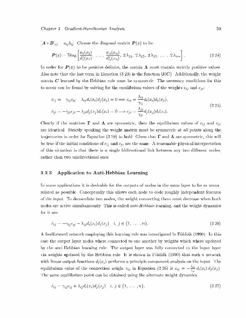
Chapter �� Gradient�Hamiltonian Analysis ��
�A �B�ij � aijbij� Choose the diagonal matrix P �z� to be
P �z� � Diag
�a��x��
d ���x��� � � � �
an�xn�
d �n�xn�� ����� ����� ����� � � � � ��nn
�� ������
In order for P �z� to be positive de�nite� the matrix � must contain strictly positive values�
Also note that the last term in Equation ������ is the function U�C�� Additionally� the weight
matrix C learned by the Hebbian rule must be symmetric� The necessary conditions for this
to occur can be found by solving for the equilibrium values of the weights cij and cji�
�cij � ��ijcij � �ijdi�xi�dj�xj� � � �� cij ��ij
�ijdi�xi�dj�xj��
�cji � ��jicji � �jidj�xj�di�xi� � � �� cji ��ji
�jidj�xj�di�xi��
������
Clearly if the matrices � and � are symmetric� then the equilibrium values of cij and cji
are identical� Strictly speaking the weight matrix must be symmetric at all points along the
trajectories in order for Equation ������ to hold� Given that � and � are symmetric� this will
be true if the initial conditions of cij and cji are the same� A reasonable physical interpretation
of this situation is that there is a single bidirectional link between any two di�erent nodes�
rather than two unidirectional ones�
����� Application to Anti Hebbian Learning
In some applications it is desirable for the outputs of nodes in the same layer to be as uncor�
related as possible� Conceptually this allows each node to code roughly independent features
of the input� To decorrelate two nodes� the weight connecting them must decrease when both
nodes are active simultaneously� This is called anti�Hebbian learning� and the weight dynamics
for it are
�cij � ��ijcij � �ijdi�xi�dj�xj� i� j � f�� � � � �ng� ������
A feedforward network employing this learning rule was investigated in F!oldi�ak ������� In this
case the output layer nodes where connected to one another by weights which where updated
by the anti�Hebbian learning rule� The output layer was fully connected to the input layer
via weights updated by the Hebbian rule� It is shown in F!oldi�ak ������ that such a network
with linear output functions di�xi� performs a principle component analysis on the input� The
equilibrium value of the connection weight cij in Equation ������ is cij � �ij�ij
di�xi� dj�xj��
The same equilibrium point can be obtained using the alternate weight dynamics
�cij � �ijcij � �ijdi�xi�dj�xj� i� j � f�� � � � �ng� ������
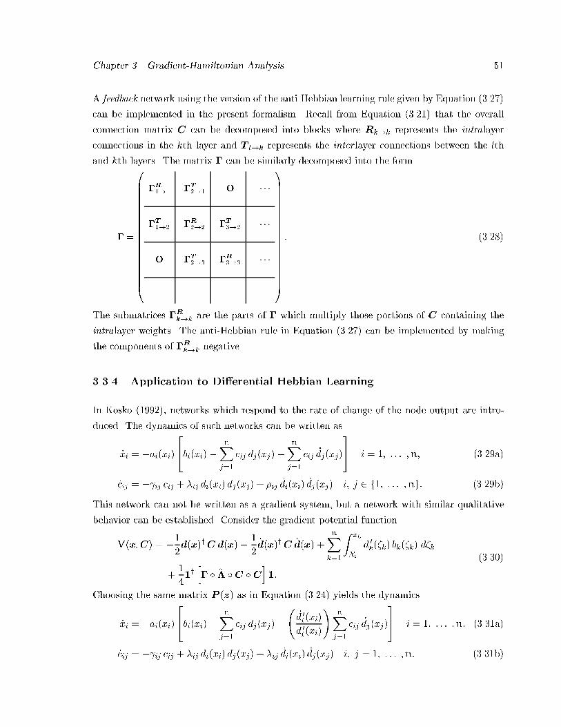
Chapter �� Gradient�Hamiltonian Analysis ��
A feedback network using the version of the anti�Hebbian learning rule given by Equation ������
can be implemented in the present formalism� Recall from Equation ������ that the overall
connection matrix C can be decomposed into blocks where Rk�k represents the intralayer
connections in the kth layer and T l�k represents the inter layer connections between the lth
and kth layers� The matrix � can be similarly decomposed into the form
�
�BBBBBBBBBBBBBBBBBB�
�R��� �T��� O � � �
�T��� �R��� �T��� � � �
O �T��� �R��� � � �
������
���� � �
�CCCCCCCCCCCCCCCCCCA
� ������
The submatrices �Rk�k are the parts of � which multiply those portions of C containing the
intralayer weights� The anti�Hebbian rule in Equation ������ can be implemented by making
the components of �Rk�k negative�
����� Application to Di�erential Hebbian Learning
In Kosko ������� networks which respond to the rate of change of the node output are intro�
duced� The dynamics of such networks can be written as
�xi � �ai�xi� �bi�xi�� nX
j��
cij dj�xj��nXj��
cij �dj�xj�
�� i � �� � � � �n� �����a�
�cij � ��ij cij � �ij di�xi� dj�xj� � �ij �di�xi� �dj�xj� i� j � f�� � � � �ng� �����b�
This network can not be written as a gradient system� but a network with similar qualitative
behavior can be established� Consider the gradient potential function
V�x�C� � ��
�d�x�yC d�x�� �
��d�x�yC �d�x� �
nXk��
Z xk
Xid �k��k� bk��k� d�k
��
��yh� � %� �C �C
i��
������
Choosing the same matrix P �z� as in Equation ������ yields the dynamics
�xi � �ai�xi� �bi�xi�� nX
j��
cij dj�xj���
�d �i �xi�d �i �xi�
�nXj��
cij �dj�xj�
�� i � �� � � � �n� �����a�
�cij � ��ij cij � �ij di�xi� dj�xj� � �ij �di�xi� �dj�xj� i� j � �� � � � �n� �����b�
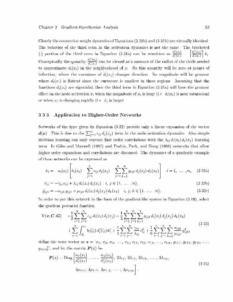
Chapter �� Gradient�Hamiltonian Analysis ��
Clearly the connection weight dynamics of Equations �����b� and �����b� are virtually identical�
The behavior of the third term in the activation dynamics is not the same� The bracketed
��� portion of the third term in Equation �����a� can be rewritten asd �i �xid �i �xi
�hd ��i �xid �i �xi
i�xi�
Conceptually the quantityd ��i �xid �i �xi
can be viewed as a measure of the radius of the circle needed
to approximate di�xi� in the neighborhood of xi� So this quantity will be zero at points of
in"ection� where the curvature of di�xi� changes direction� Its magnitude will be greatest
where di�xi� is "attest since the curvature is smallest in these regions� Assuming that the
functions di�xi� are sigmoidal� then the third term in Equation �����a� will have the greatest
e�ect on the node activation xi when the magnitude of xi is large �i�e� di�xi� is near saturation�
or when xi is changing rapidly �i�e� �xi is large��
����� Application to Higher Order Networks
Networks of the type given by Equation ������ provide only a linear expansion of the vector
d�x�� This is due to thePn
j�� cij dj�xj� term in the node activation dynamics� Also simple
Hebbian learning can only capture �rst order correlations with the �ij di�xi� dj�xj� learning
term� In Giles and Maxwell ������ and Psaltis� Park� and Hong ������ networks that allow
higher order expansions and correlations are discussed� The dynamics of a quadratic example
of these networks can be expressed as
�xi � �ai�xi� �bi�xi�� nX
j��
cij dj�xj��nXj��
nXk��
gijk dj�xj� dk�xk�
�� i � �� � � � �n� �����a�
�cij � ��ij cij � �ij di�xi� dj�xj� i� j � f�� � � � �ng� �����b�
�gijk � ��ijk gijk � ijk di�xi� dj�xj� dk�xk� i� j� k � f�� � � � �ng� �����c�
In order to put this network in the form of the gradient�like system in Equation ������� select
the gradient potential function
V�x�C�G� � ��
�
nXi��
nXj��
cij di�xi� dj�xj�� �
�
nXi��
nXj��
nXk��
gijk di�xi� dj�xj� dk�xk�
�nXi��
Z xi
Xibi��i� d
�i ��i�d� �
�
�
nXi��
nXj��
�ij
�ijc�ij �
�
�
nXi��
nXj��
nXk��
�ijk
ijkg�ijk�
������
de�ne the state vector as z � �x�� x�� x�� � � � � xn� c��� c��� c��� � � � � cnn� g���� g���� g���� � � � �
gnnn�y� and let the matrix P �z� be
P �z� � Diag
�a��x��
d ���x��� � � � �
an�xn�
d �n�xn�� ����� ����� ����� � � � � ��nn�
����� ����� ����� � � � � �nnn
��
������
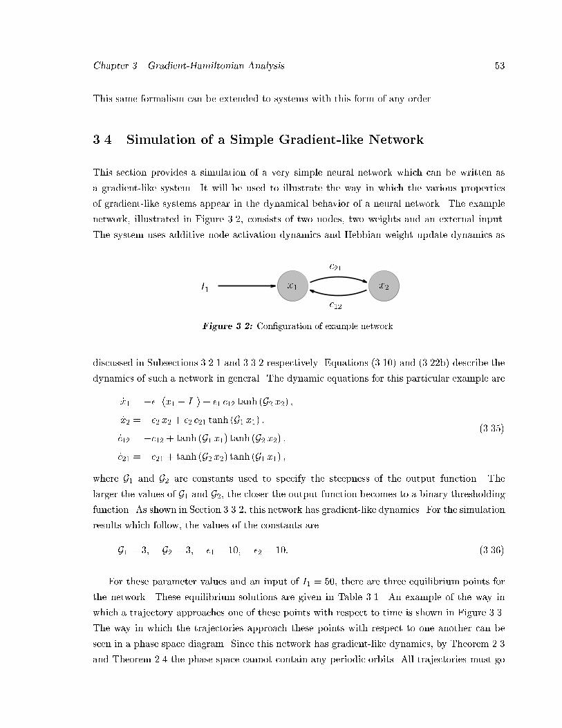
Chapter �� Gradient�Hamiltonian Analysis ��
This same formalism can be extended to systems with this form of any order�
��� Simulation of a Simple Gradient�like Network
This section provides a simulation of a very simple neural network which can be written as
a gradient�like system� It will be used to illustrate the way in which the various properties
of gradient�like systems appear in the dynamical behavior of a neural network� The example
network� illustrated in Figure ���� consists of two nodes� two weights and an external input�
The system uses additive node activation dynamics and Hebbian weight update dynamics as
I� x� x�
c��
c��
Figure ���� Con�guration of example network�
discussed in Subsections ����� and ����� respectively� Equations ������ and �����b� describe the
dynamics of such a network in general� The dynamic equations for this particular example are
�x� � �� �x� � I�� � � c�� tanh �G� x�� ��x� � �� x� � � c�� tanh �G� x�� ��c�� � �c�� � tanh �G� x�� tanh �G� x�� ��c�� � �c�� � tanh �G� x�� tanh �G� x�� �
������
where G� and G� are constants used to specify the steepness of the output function� The
larger the values of G� and G�� the closer the output function becomes to a binary thresholding
function� As shown in Section ������ this network has gradient�like dynamics� For the simulation
results which follow� the values of the constants are
G� � �� G� � �� � � ��� � � ��� ������
For these parameter values and an input of I� � ��� there are three equilibrium points for
the network� These equilibrium solutions are given in Table ���� An example of the way in
which a trajectory approaches one of these points with respect to time is shown in Figure ����
The way in which the trajectories approach these points with respect to one another can be
seen in a phase space diagram� Since this network has gradient�like dynamics� by Theorem ���
and Theorem ��� the phase space cannot contain any periodic orbits� All trajectories must go
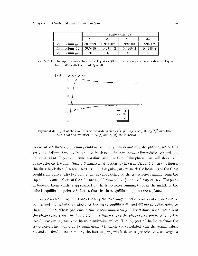
Chapter �� Gradient�Hamiltonian Analysis ��
state variablesx� x� c�� c��
Equilibrium &� ������� �������� �������� ��������
Equilibrium &� ������� ��������� ��������� ���������Equilibrium &� �� � � �
Table ���� The equilibrium solutions of Equation ������ using the parameter values in Equa�tion ������ with the input I� ���
1 2 3 4
-40
-20
20
40
60
t
fx��t�� x��t�� c���t� g
c��
x�
x�
Figure ���� A plot of the evolution of the state variables �x��t�� x��t�� c���t�� c���t��y
over time�Note that the evolution of c���t� and c���t� are identical�
to one of the three equilibrium points or to in�nity� Unfortunately� the phase space of this
system is ��dimensional� which can not be drawn� However because the weights� c�� and c���
are identical at all points in time� a ��dimensional section of the phase space will show most
of the relevant features� Such a ��dimensional section is shown in Figure ���� In this �gure�
the three black dots clustered together in a triangular pattern mark the locations of the three
equilibrium points� The two points that are approached by the trajectories running along the
top and bottom surfaces of the cube are equilibrium points &� and &� respectively� The point
in between them which is approached by the trajectories running through the middle of the
cube is equilibrium point &�� Notice that the three equilibrium points are coplanar�
It appears from Figure ��� that the trajectories change directions rather abruptly at some
points� and that all of the trajectories leading to equilibria &� and &� merge before going to
these equilibria� These phenomena can be seen more clearly in the ��dimensional sections of
the phase space shown in Figure ���� This �gure shows the phase space projected onto the
two dimensions representing the node activation values� The top part of the �gure shows the
trajectories which converge to equilibrium &�� which was calculated with the weight values
c�� and c�� �xed at ��� Similarly the bottom part� which shows trajectories that converge to
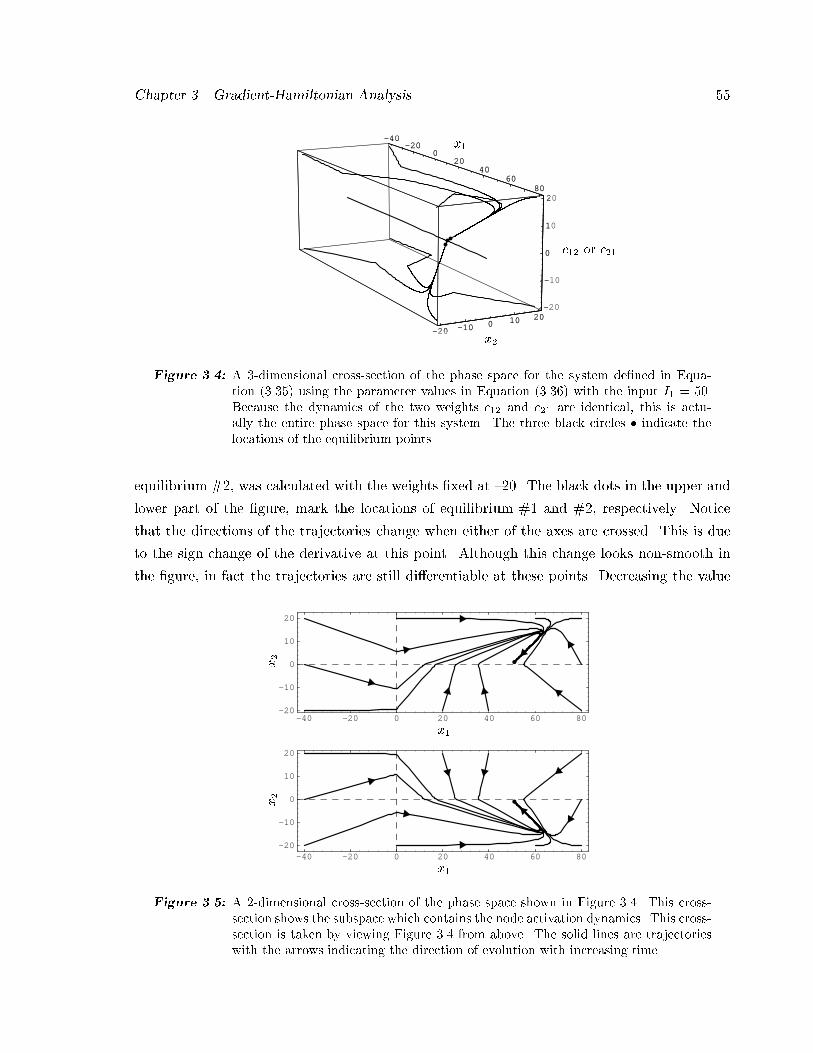
Chapter �� Gradient�Hamiltonian Analysis ��
-40-20
020
4060
80
-20 -10 0 10 20-20
-10
0
10
20
-40-20
020
4060
80
-20 -10 0 10 20-2
-
0
1
2
x�
x�
c�� or c��
x�
x�
c�� or c��
Figure ���� A ��dimensional cross�section of the phase space for the system de�ned in Equa�tion ������ using the parameter values in Equation ������ with the input I� ���Because the dynamics of the two weights c�� and c�� are identical� this is actu�ally the entire phase space for this system� The three black circles � indicate thelocations of the equilibrium points�
equilibrium &�� was calculated with the weights �xed at ��� The black dots in the upper and
lower part of the �gure� mark the locations of equilibrium &� and &�� respectively� Notice
that the directions of the trajectories change when either of the axes are crossed� This is due
to the sign change of the derivative at this point� Although this change looks non�smooth in
the �gure� in fact the trajectories are still di�erentiable at these points� Decreasing the value
-40 -20 0 20 40 60 80-20
-10
0
10
20
x�
x�
-40 -20 0 20 40 60 80-20
-10
0
10
20
x�
x�
Figure ���� A ��dimensional cross�section of the phase space shown in Figure ���� This cross�section shows the subspace which contains the node activation dynamics� This cross�section is taken by viewing Figure ��� from above� The solid lines are trajectorieswith the arrows indicating the direction of evolution with increasing time�

Chapter �� Gradient�Hamiltonian Analysis ��
of G� and G� makes these transitions more gradual�
If the input I� is negative �e�g� ��� then the phase space diagram is identical to Figure ����
except the signs of the numbers on the x� and x� axes are reversed� The equilibrium locations
for this system are given in Table ���� Note that the three equilibria for I� � ��� do not lie on
state variablesx� x� c�� c��
Equilibrium &� �������� ��������� �������� ��������
Equilibrium &� �������� �������� ��������� ���������Equilibrium &� ��� � � �
Table ���� The equilibrium solutions of Equation ������ using the parameter values in Equa�tion ������ with the input I� ����
the same plane as those for I� � ��� in fact the two planes are perpendicular� It was observed
that smaller values of G� and G� caused equilibria &� and &� to move closer to equilibrium
&�� In the limit as G�� G� � �� only equilibrium &� exists� Making the values larger has the
opposite e�ect� however the equilibrium values of x�� c��� and c�� at equilibria &� and &� are
limited to jx�j � jc��j � jc��j � � as G�� G� ���
As discussed in Subsection ������ the type of equilibrium point may be determined by �nding
the eigenvalues of the Jacobian of the system evaluated at each equilibrium point� Because
the system is gradient�like� Theorem ��� shows that the eigenvalues of the Jacobian at every
equilibrium point must be real valued� Furthermore� the Jacobian must be diagonalizable at
each equilibrium point� For this system the Jacobian is given by
JG
�BBB�
� � �� c�� sech� ��x�� � tanh ��x�� �
�� c�� sech� ��x�� � � � � tanh ��x��
� sech� ��x�� tanh ��x�� � sech� ��x�� tanh ��x�� � �
� sech� ��x�� tanh ��x�� � sech� ��x�� tanh ��x�� � �
�CCCA � ������
The eigenvalues of the Jacobian at each of the three equilibrium points are given in Table ����
Since all of the eigenvalues of the Jacobian are negative at equilibrium points &� and &�� both
eigenvalues�� �� �� ��
Equilibrium &� ��� ��������� �������� ��Equilibrium &� ��� ��������� �������� ��Equilibrium &� �� ��� ������� ��������
Table ���� The eigenvalues of the Jacobian matrix de�ned in Equation ������ at the equilibriumpoints shown in Table �� �
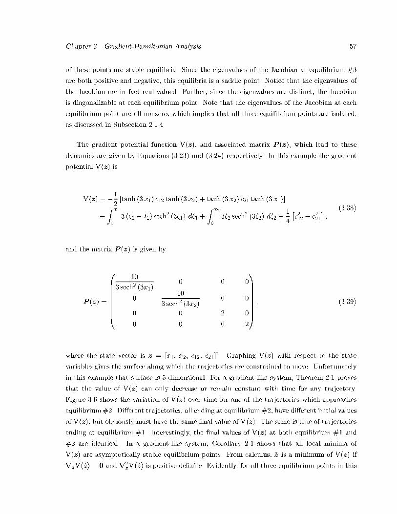
Chapter �� Gradient�Hamiltonian Analysis ��
of these points are stable equilibria� Since the eigenvalues of the Jacobian at equilibrium &�
are both positive and negative� this equilibria is a saddle point� Notice that the eigenvalues of
the Jacobian are in fact real valued� Further� since the eigenvalues are distinct� the Jacobian
is diagonalizable at each equilibrium point� Note that the eigenvalues of the Jacobian at each
equilibrium point are all nonzero� which implies that all three equilibrium points are isolated�
as discussed in Subsection ������
The gradient potential function V�z�� and associated matrix P �z�� which lead to these
dynamics are given by Equations ������ and ������ respectively� In this example the gradient
potential V�z� is
V�z� � ��
��tanh ��x�� c�� tanh ��x�� � tanh ��x�� c�� tanh ��x���
�
Z x�
�� ��� � I�� sech
� ����� d�� �
Z x�
���� sech
� ����� d�� ��
�
�c��� � c���
��
������
and the matrix P �z� is given by
P �z� �
BBBBBBB�
��
� sech� ��x��� � �
���
� sech� ��x��� �
� � � �
� � � �
�CCCCCCCA� ������
where the state vector is z � �x�� x�� c��� c���y� Graphing V�z� with respect to the state
variables gives the surface along which the trajectories are constrained to move� Unfortunately
in this example that surface is ��dimensional� For a gradient�like system� Theorem ��� proves
that the value of V�z� can only decrease or remain constant with time for any trajectory�
Figure ��� shows the variation of V�z� over time for one of the trajectories which approaches
equilibrium&�� Di�erent trajectories� all ending at equilibrium&�� have di�erent initial values
of V�z�� but obviously must have the same �nal value of V�z�� The same is true of trajectories
ending at equilibrium &�� Interestingly� the �nal values of V�z� at both equilibrium &� and
&� are identical� In a gradient�like system� Corollary ��� shows that all local minima of
V�z� are asymptotically stable equilibrium points� From calculus� %z is a minimum of V�z� if
rzV�%z� � and r�zV�%z� is positive de�nite� Evidently� for all three equilibrium points in this
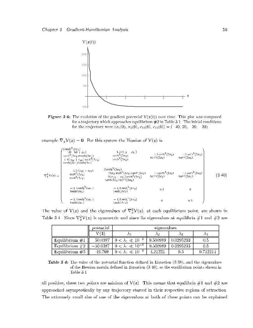
Chapter �� Gradient�Hamiltonian Analysis ��
1 2 3 4 5
-50
50
100
150
200
t
V�z�t��
Figure ���� The evolution of the gradient potential V�z�t�� over time� This plot was computedfor a trajectory which approaches equilibrium �� in Table �� � The initial conditionsfor the trajectory were �x����� x����� c������ c������ ����� ��� ���� �����
example rzV��z� � � For this system the Hessian of V�z� is
r�
zV�z �
�BBBBBBBBBBBBBBBBBBBBBBBBBB�
� sech���x�
� ����� � x�
sech���x� tanh��x�
� ��c�� � c�� sech���x�
tanh��x� tanh��x�
� ��� �c�� � c��
sech���x�
sech���x�
� ��� sech���x�tanh��x�
� ��� sech���x�tanh��x�
� ��� �c�� � c��
sech���x�
sech���x�
� sech���x�
� �x� sech���x� tanh��x�
� � �c�� � c�� sech���x�
tanh��x� tanh��x�
� ��� sech���x�tanh��x�
� ��� sech���x�tanh��x�
� ��� sech���x�
tanh��x�� ��� sech
���x�
tanh��x���� �
� ��� sech���x�tanh��x�
� ��� sech���x�tanh��x�
� ���
�CCCCCCCCCCCCCCCCCCCCCCCCCCA
� ������
The value of V�z� and the eigenvalues of r�zV�z�� at each equilibrium point� are shown in
Table ���� Since r�zV�z� is symmetric and since its eigenvalues at equilibria &� and &� are
potential eigenvaluesV��z� �� �� �� ��
Equilibrium &� �������� � � �� � ���� �������� ��������� ���
Equilibrium &� �������� � � �� � ���� �������� ��������� ���
Equilibrium &� ������� � � �� � ���� ������� ��� ���������
Table ���� The value of the potential function de�ned in Equation ������� and the eigenvaluesof the Hessian matrix de�ned in Equation ������� at the equilibrium points shown inTable �� �
all positive� these two points are minima of V�z�� This means that equilibria &� and &� are
approached asymptotically by any trajectory started in their respective regions of attraction�
The extremely small size of one of the eigenvalues at both of these points can be explained
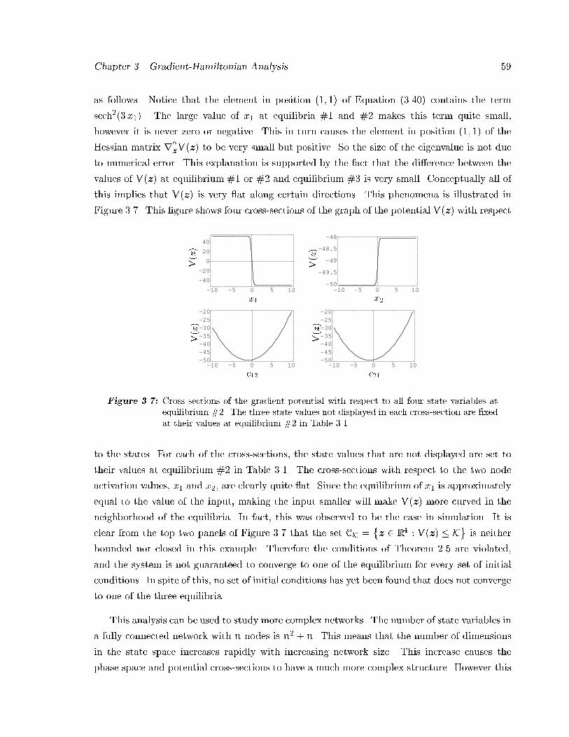
Chapter �� Gradient�Hamiltonian Analysis ��
as follows� Notice that the element in position ��� �� of Equation ������ contains the term
sech���x��� The large value of x� at equilibria &� and &� makes this term quite small�
however it is never zero or negative� This in turn causes the element in position ��� �� of the
Hessian matrix r�zV�z� to be very small but positive� So the size of the eigenvalue is not due
to numerical error� This explanation is supported by the fact that the di�erence between the
values of V�z� at equilibrium &� or &� and equilibrium &� is very small� Conceptually all of
this implies that V�z� is very "at along certain directions� This phenomena is illustrated in
Figure ���� This �gure shows four cross�sections of the graph of the potential V�z� with respect
-10 -5 0 5 10
-40
-20
0
20
40
-10 -5 0 5 10
-50
-49.5
-49
-48.5
-48
-10 -5 0 5 10-50-45-40-35-30-25-20
-10 -5 0 5 10-50-45-40-35-30-25-20
x�
V�z�
x�
V�z�
c��
V�z�
c��
V�z�
Figure ��� Cross sections of the gradient potential with respect to all four state variables atequilibrium ��� The three state values not displayed in each cross�section are �xedat their values at equilibrium �� in Table �� �
to the states� For each of the cross�sections� the state values that are not displayed are set to
their values at equilibrium &� in Table ���� The cross�sections with respect to the two node
activation values� x� and x�� are clearly quite "at� Since the equilibrium of x� is approximately
equal to the value of the input� making the input smaller will make V�z� more curved in the
neighborhood of the equilibria� In fact� this was observed to be the case in simulation� It is
clear from the top two panels of Figure ��� that the set CK ��z � R� � V�z� � K� is neither
bounded nor closed in this example� Therefore the conditions of Theorem ��� are violated�
and the system is not guaranteed to converge to one of the equilibrium for every set of initial
conditions� In spite of this� no set of initial conditions has yet been found that does not converge
to one of the three equilibria�
This analysis can be used to study more complex networks� The number of state variables in
a fully connected network with n nodes is n� � n� This means that the number of dimensions
in the state space increases rapidly with increasing network size� This increase causes the
phase space and potential cross�sections to have a much more complex structure� However this

Chapter �� Gradient�Hamiltonian Analysis ��
formalism is still an extremely useful one for analyzing high dimensional networks�
��� Review of Gradient�Hamiltonian Decomposition Results
In this section the results from Mendes and Duarte ������� Duarte and Mendes ������� and
Mendes and Duarte ������ will be reviewed� It was proven in Mendes and Duarte ������ that
any vector �eld f on a manifold M can be locally decomposed into the sum of one gradient
system and �n � �� Hamiltonian systems� where n is the local dimension of the manifold�
Further it was proved that if either the Riemannian metric or the symplectic form can be
speci�cally chosen to match the vector �eld f � then the system dynamics can be decomposed
into one gradient system and one Hamiltonian system� regardless of the dimension of M� The
main result of that paper is stated in the following lemma�
Lemma ��� �Mendes and Duarte � Given a smooth manifold M� By de�nition� for every
point x �M there exists a neighborhood N M which is homeomorphic to En� Assume that the
local value of n is always an even number� For every neighborhood N there exists a Riemannian
metric D � Rn Rn � R and �n��� symplectic forms Fi � Rn Rn � R such that every vector
�eld f de�ned on N can be decomposed into one gradient and �n��� Hamiltonian vector �elds�
For the de�nitions of Riemannian metric and symplectic form� see Appendix A� This result
can be applied to systems where n is odd by embedding the system in an �n� ���dimensional
manifold� This result means that any system of di�erential equations �z � f�z� can be written
in the form
�z � �rzV�z� �
nXi��
rzHi�z�� ������
in the local region z � N M� The proof given in Mendes and Duarte ������ is constructive�
so in principle the local gradient and Hamiltonian potential functions can be found for any
system� However� solving the necessary equations to �nd these potentials may be very di�cult�
For instance� the gradient potential is the solution to the Poisson equation� r�zV�z� � r�f�z��
Note that if r f�z� � then the system can be represented by the gradient component
alone� while if r � f�z� � � the system can be described using only Hamiltonian components�
Equation ������ can be interpreted as saying that any dynamical system consists of a conser�
vative �e�g� Hamiltonian� system perturbed by a dissipative �e�g� gradient� system� Of course�
there is no guarantee that the dissipative system is a small perturbation of the conservative
system� in fact it may dominate the system behavior� This being the case� it is more prof�
itable to view the dissipative portion as a deformation of the conservative system� rather than
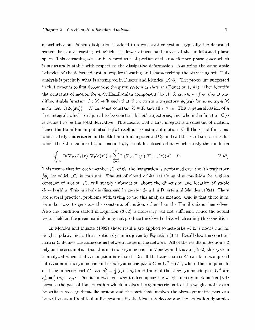
Chapter �� Gradient�Hamiltonian Analysis ��
a perturbation� When dissipation is added to a conservative system� typically the deformed
system has an attracting set which is a lower dimensional subset of the undeformed phase
space� This attracting set can be viewed as that portion of the undeformed phase space which
is structurally stable with respect to the dissipative deformation� Analyzing the asymptotic
behavior of the deformed system requires locating and characterizing the attracting set� This
analysis is precisely what is attempted in Duarte and Mendes ������� The procedure suggested
in that paper is to �rst decompose the given system as shown in Equation ������� Then identify
the constants of motion for each Hamiltonian component Hi�z�� A constant of motion is any
di�erentiable function C � M� R such that there exists a trajectory �t�x�� for some x� �Msuch that C��t�x��� � K for some constant K � R and all t � t�� This a generalization of a
�rst integral� which is required to be constant for all trajectories� and where the function C���is de�ned to be the total derivative� This means that a �rst integral is a constant of motion�
hence the Hamiltonian potential Hi�z� itself is a constant of motion� Call the set of functions
which satisfy this criteria for the ith Hamiltonian potential Ci� and call the set of trajectories for
which the kth member of Ci is constant k'i� Look for closed orbits which satisfy the conditionIlk�i
D�rz kC��z��rzV�z�� �
nXi��
Fi�rz kCi�z��rzHi�z�� dt � �� ������
This means that for each member kCi of Ci� the integration is performed over the lth trajectorylk�i for which kCi is constant� The set of closed orbits satisfying this condition for a given
constant of motion kCi will supply information about the dimension and location of stable
closed orbits� This analysis is discussed in greater detail in Duarte and Mendes ������� There
are several practical problems with trying to use this analysis method� One is that there is no
formulaic way to generate the constants of motion� other than the Hamiltonians themselves�
Also the condition stated in Equation ������ is necessary but not su�cient� hence the actual
vector �eld on the given manifold may not produce the closed orbits which satisfy this condition�
In Mendes and Duarte ������ these results are applied to networks with n nodes and no
weight update� and with activation dynamics given by Equation ������ Recall that the constant
matrix C de�nes the connections between nodes in the network� All of the results in Section ���
rely on the assumption that this matrix is symmetric� In Mendes and Duarte ������ this system
is analyzed when that assumption is relaxed� Recall that any matrix C can be decomposed
into a sum of its symmetric and skew�symmetric parts C � CS �CA� where the components
of the symmetric part CS are cSij ��� �cij � cji� and those of the skew�symmetric part CA are
cAij ��� �cij � cji�� This is an excellent way to decompose the weight matrix in Equation �����
because the part of the activation which involves the symmetric part of the weight matrix can
be written as a gradient�like system and the part that involves the skew�symmetric part can
be written as a Hamiltonian�like system� So the idea is to decompose the activation dynamics
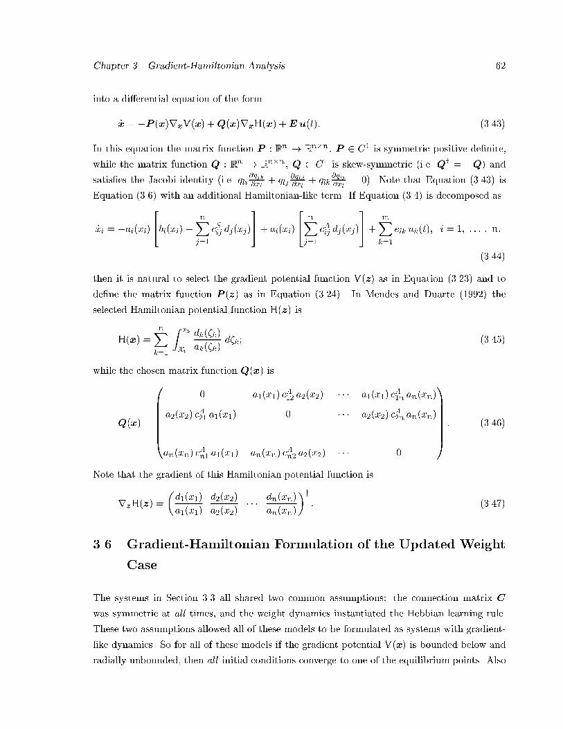
Chapter �� Gradient�Hamiltonian Analysis ��
into a di�erential equation of the form
�x � �P �x�rxV�x� �Q�x�rxH�x� �Eu�t�� ������
In this equation the matrix function P � Rn � Rn�n � P � C� is symmetric positive de�nite�
while the matrix function Q � Rn � Rn�n � Q � C� is skew�symmetric �i�e� Qy � �Q� and
satis�es the Jacobi identity �i�e� qli�qjk�xl
� qlj�qki�xl
� qlk�qij�xl
� ��� Note that Equation ������ is
Equation ����� with an additional Hamiltonian�like term� If Equation ����� is decomposed as
�xi � �ai�xi� �bi�xi�� nX
j��
cSij dj�xj�
��� ai�xi�
� nXj��
cAij dj�xj�
���
mXk��
eik uk�t�� i � �� � � � � n�
������
then it is natural to select the gradient potential function V�z� as in Equation ������ and to
de�ne the matrix function P �z� as in Equation ������� In Mendes and Duarte ������ the
selected Hamiltonian potential function H�z� is
H�x� �
nXk��
Z xk
Xi
dk��k�
ak��k�d�k� ������
while the chosen matrix function Q�x� is
Q�x� �
BBBBBB�
� a��x�� cA�� a��x�� � � � a��x�� c
A�n an�xn�
a��x�� cA�� a��x�� � � � � a��x�� c
A�n an�xn�
������
� � ����
an�xn� cAn� a��x�� an�xn� c
An� a��x�� � � � �
�CCCCCCA� ������
Note that the gradient of this Hamiltonian potential function is
rzH�z� �
�d��x��
a��x��
d��x��
a��x��� � � dn�xn�
an�xn�
�y� ������
�� Gradient�Hamiltonian Formulation of the Updated Weight
Case
The systems in Section ��� all shared two common assumptions� the connection matrix C
was symmetric at all times� and the weight dynamics instantiated the Hebbian learning rule�
These two assumptions allowed all of these models to be formulated as systems with gradient�
like dynamics� So for all of these models if the gradient potential V�x� is bounded below and
radially unbounded� then all initial conditions converge to one of the equilibrium points� Also
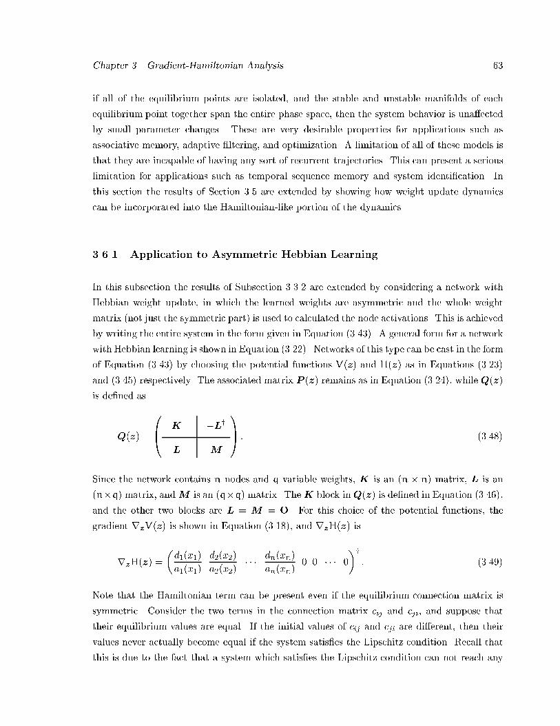
Chapter �� Gradient�Hamiltonian Analysis ��
if all of the equilibrium points are isolated� and the stable and unstable manifolds of each
equilibrium point together span the entire phase space� then the system behavior is una�ected
by small parameter changes� These are very desirable properties for applications such as
associative memory� adaptive �ltering� and optimization� A limitation of all of these models is
that they are incapable of having any sort of recurrent trajectories� This can present a serious
limitation for applications such as temporal sequence memory and system identi�cation� In
this section the results of Section ��� are extended by showing how weight update dynamics
can be incorporated into the Hamiltonian�like portion of the dynamics�
����� Application to Asymmetric Hebbian Learning
In this subsection the results of Subsection ����� are extended by considering a network with
Hebbian weight update� in which the learned weights are asymmetric and the whole weight
matrix �not just the symmetric part� is used to calculated the node activations� This is achieved
by writing the entire system in the form given in Equation ������� A general form for a network
with Hebbian learning is shown in Equation ������� Networks of this type can be cast in the form
of Equation ������ by choosing the potential functions V�z� and H�z� as in Equations ������
and ������ respectively� The associated matrix P �z� remains as in Equation ������� while Q�z�
is de�ned as
Q�z� �
B� K �Ly
L M
�CA � ������
Since the network contains n nodes and q variable weights� K is an �n n� matrix� L is an
�n q� matrix� andM is an �q q� matrix� TheK block inQ�z� is de�ned in Equation �������
and the other two blocks are L � M � O� For this choice of the potential functions� the
gradient rzV�z� is shown in Equation ������� and rzH�z� is
rzH�z� �
�d��x��
a��x��
d��x��
a��x��� � � dn�xn�
an�xn�� � � � � �
�y� ������
Note that the Hamiltonian term can be present even if the equilibrium connection matrix is
symmetric� Consider the two terms in the connection matrix cij and cji� and suppose that
their equilibrium values are equal� If the initial values of cij and cji are di�erent� then their
values never actually become equal if the system satis�es the Lipschitz condition� Recall that
this is due to the fact that a system which satis�es the Lipschitz condition can not reach any
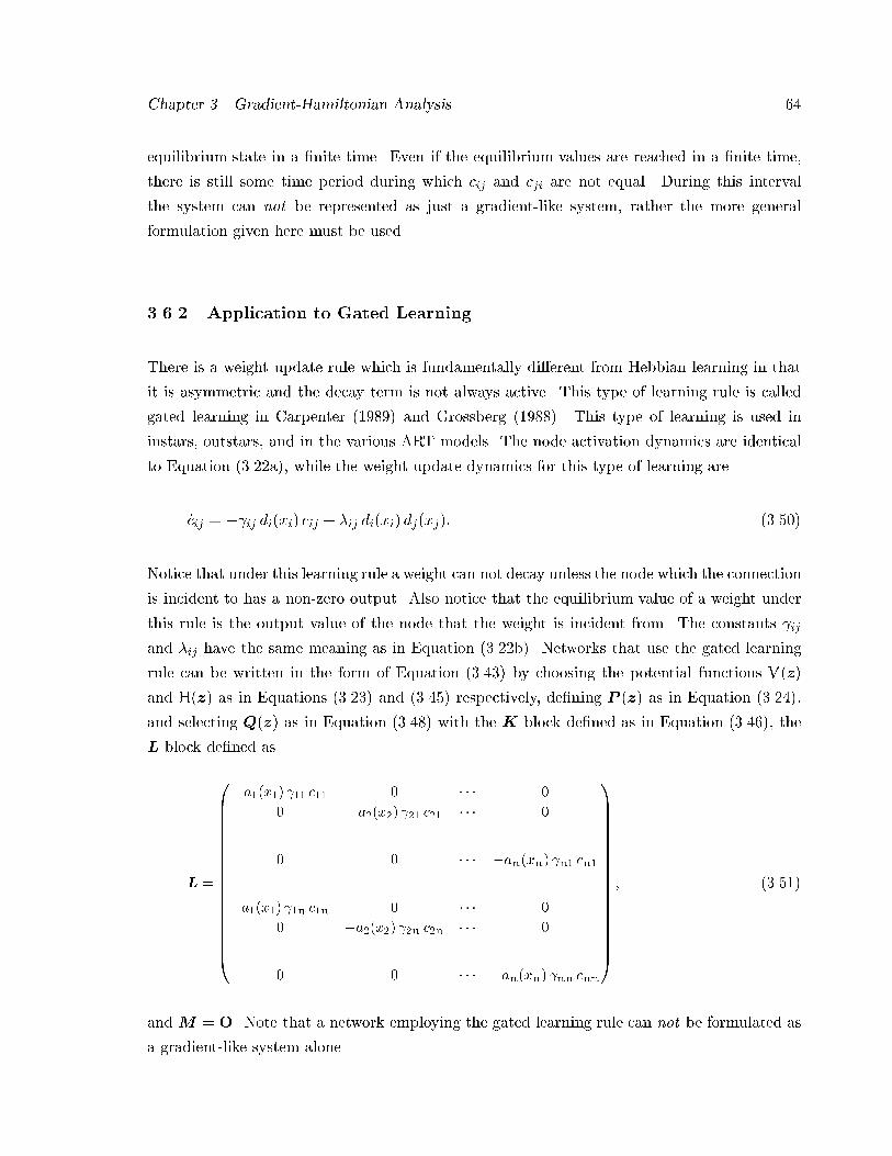
Chapter �� Gradient�Hamiltonian Analysis ��
equilibrium state in a �nite time� Even if the equilibrium values are reached in a �nite time�
there is still some time period during which cij and cji are not equal� During this interval
the system can not be represented as just a gradient�like system� rather the more general
formulation given here must be used�
����� Application to Gated Learning
There is a weight update rule which is fundamentally di�erent from Hebbian learning in that
it is asymmetric and the decay term is not always active� This type of learning rule is called
gated learning in Carpenter ������ and Grossberg ������� This type of learning is used in
instars� outstars� and in the various ART models� The node activation dynamics are identical
to Equation �����a�� while the weight update dynamics for this type of learning are
�cij � ��ij di�xi� cij � �ij di�xi� dj�xj�� ������
Notice that under this learning rule a weight can not decay unless the node which the connection
is incident to has a non�zero output� Also notice that the equilibrium value of a weight under
this rule is the output value of the node that the weight is incident from� The constants �ij
and �ij have the same meaning as in Equation �����b�� Networks that use the gated learning
rule can be written in the form of Equation ������ by choosing the potential functions V�z�
and H�z� as in Equations ������ and ������ respectively� de�ning P �z� as in Equation �������
and selecting Q�z� as in Equation ������ with the K block de�ned as in Equation ������� the
L block de�ned as
L
�BBBBBBBBBBBBBBBBB�
�a��x�� ��� c�� � � � � �
� �a��x�� ��� c�� � � � ����
���� � �
���
� � � � � �an�xn� �n� cn����
���� � �
���
�a��x�� ��n c�n � � � � �
� �a��x�� ��n c�n � � � ����
���� � �
���
� � � � � �an�xn� �nn cnn
�CCCCCCCCCCCCCCCCCA
� ������
and M � O� Note that a network employing the gated learning rule can not be formulated as
a gradient�like system alone�
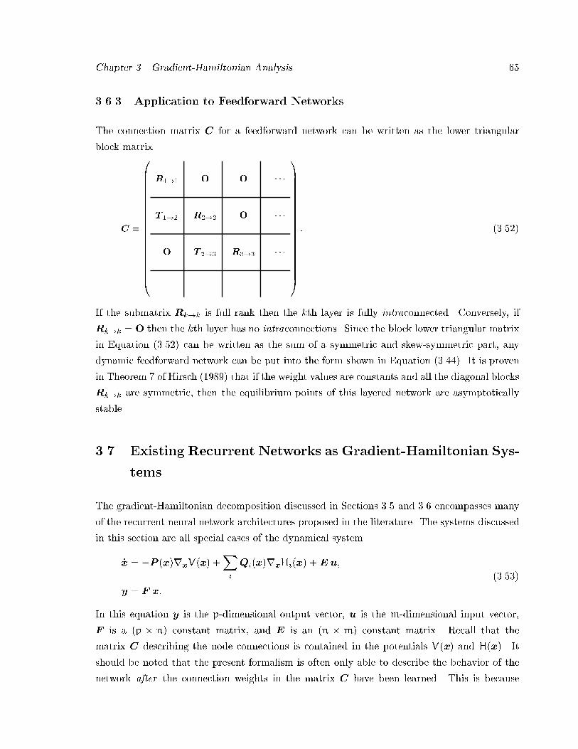
Chapter �� Gradient�Hamiltonian Analysis ��
����� Application to Feedforward Networks
The connection matrix C for a feedforward network can be written as the lower triangular
block matrix
C
�BBBBBBBBBBBBBBBBBB�
R��� O O � � �
T ��� R��� O � � �
O T ��� R��� � � �
������
���� � �
�CCCCCCCCCCCCCCCCCCA
� ������
If the submatrix Rk�k is full rank then the kth layer is fully intraconnected� Conversely� if
Rk�k � O then the kth layer has no intraconnections� Since the block lower triangular matrix
in Equation ������ can be written as the sum of a symmetric and skew�symmetric part� any
dynamic feedforward network can be put into the form shown in Equation ������� It is proven
in Theorem � of Hirsch ������ that if the weight values are constants and all the diagonal blocks
Rk�k are symmetric� then the equilibrium points of this layered network are asymptotically
stable�
�� Existing Recurrent Networks as Gradient�Hamiltonian Sys�
tems
The gradient�Hamiltonian decomposition discussed in Sections ��� and ��� encompasses many
of the recurrent neural network architectures proposed in the literature� The systems discussed
in this section are all special cases of the dynamical system
�x � �P �x�rxV�x� �Xi
Qi�x�rxHi�x� �Eu�
y � F x�
������
In this equation y is the p�dimensional output vector� u is the m�dimensional input vector�
F is a �p n� constant matrix� and E is an �n m� constant matrix� Recall that the
matrix C describing the node connections is contained in the potentials V�x� and H�x�� It
should be noted that the present formalism is often only able to describe the behavior of the
network after the connection weights in the matrix C have been learned� This is because
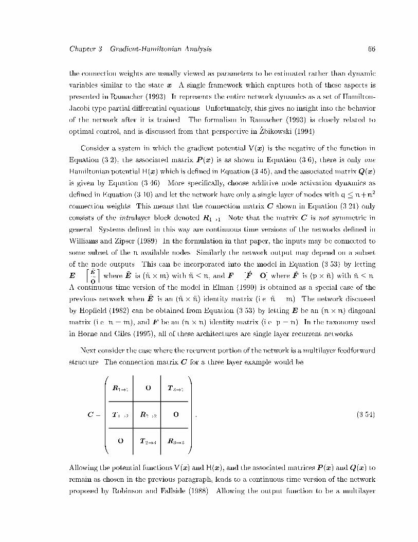
Chapter �� Gradient�Hamiltonian Analysis ��
the connection weights are usually viewed as parameters to be estimated rather than dynamic
variables similar to the state x� A single framework which captures both of these aspects is
presented in Ramacher ������� It represents the entire network dynamics as a set of Hamilton�
Jacobi type partial di�erential equations� Unfortunately� this gives no insight into the behavior
of the network after it is trained� The formalism in Ramacher ������ is closely related to
optimal control� and is discussed from that perspective in �Zbikowski �������
Consider a system in which the gradient potential V�x� is the negative of the function in
Equation ������ the associated matrix P �x� is as shown in Equation ������ there is only one
Hamiltonian potentialH�x� which is de�ned in Equation ������� and the associated matrixQ�x�
is given by Equation ������� More speci�cally� choose additive node activation dynamics as
de�ned in Equation ������ and let the network have only a single layer of nodes with q � n�n�
connection weights� This means that the connection matrix C shown in Equation ������ only
consists of the intralayer block denoted R���� Note that the matrix C is not symmetric in
general� Systems de�ned in this way are continuous time versions of the networks de�ned in
Williams and Zipser ������� In the formulation in that paper� the inputs may be connected to
some subset of the n available nodes� Similarly the network output may depend on a subset
of the node outputs� This can be incorporated into the model in Equation ������ by letting
E �h
E���O
iwhere %E is �%n m� with %n � n� and F � � (F
��� O� where (F is �p (n� with (n � n�
A continuous time version of the model in Elman ������ is obtained as a special case of the
previous network when %E is an �%n %n� identity matrix �i�e� %n � m�� The network discussed
by Hop�eld ������ can be obtained from Equation ������ by letting E be an �n n� diagonal
matrix �i�e� n � m�� and F be an �n n� identity matrix �i�e� p � n�� In the taxonomy used
in Horne and Giles ������� all of these architectures are single layer recurrent networks�
Next consider the case where the recurrent portion of the network is a multilayer feedforward
structure� The connection matrix C for a three layer example would be
C
�BBBBBBBBBBBBB�
R��� O T ���
T ��� R��� O
O T ��� R���
�CCCCCCCCCCCCCA� ������
Allowing the potential functions V�x� and H�x�� and the associated matrices P �x� andQ�x� to
remain as chosen in the previous paragraph� leads to a continuous time version of the network
proposed by Robinson and Fallside ������� Allowing the output function to be a multilayer
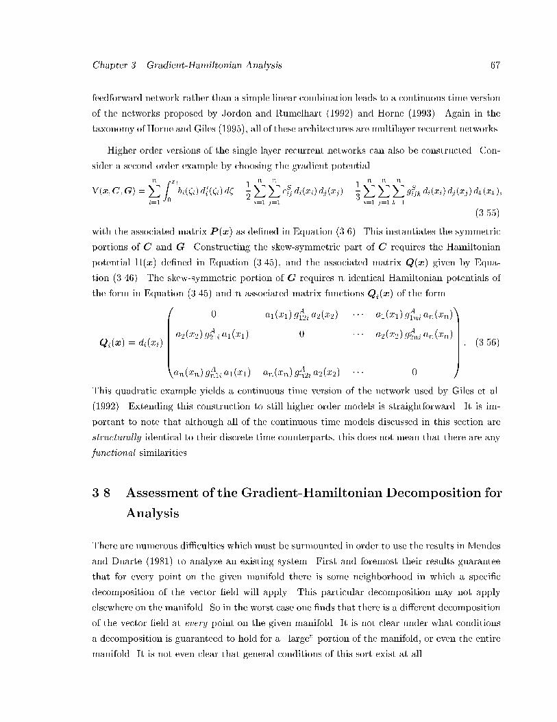
Chapter �� Gradient�Hamiltonian Analysis ��
feedforward network rather than a simple linear combination leads to a continuous time version
of the networks proposed by Jordon and Rumelhart ������ and Horne ������� Again in the
taxonomy of Horne and Giles ������� all of these architectures are multilayer recurrent networks�
Higher order versions of the single layer recurrent networks can also be constructed� Con�
sider a second order example by choosing the gradient potential
V�x�C�G�
nXi��
Z xi
�
bi��i� d�i ��i� d� �
�
nXi��
nXj��
cSij di�xi� dj�xj��
�
nXi��
nXj��
nXk��
gSijk di�xi� dj�xj� dk�xk��
������
with the associated matrix P �x� as de�ned in Equation ������ This instantiates the symmetric
portions of C and G� Constructing the skew�symmetric part of C requires the Hamiltonian
potential H�x� de�ned in Equation ������� and the associated matrix Q�x� given by Equa�
tion ������� The skew�symmetric portion of G requires n identical Hamiltonian potentials of
the form in Equation ������ and n associated matrix functions Qi�x� of the form
Qi�x� � di�xi�
BBBBBB�
� a��x�� gA��i a��x�� � � � a��x�� g
A�ni an�xn�
a��x�� gA��i a��x�� � � � � a��x�� g
A�ni an�xn�
������
� � ����
an�xn� gAn�i a��x�� an�xn� g
An�i a��x�� � � � �
�CCCCCCA� ������
This quadratic example yields a continuous time version of the network used by Giles et al�
������� Extending this construction to still higher order models is straightforward� It is im�
portant to note that although all of the continuous time models discussed in this section are
structurally identical to their discrete time counterparts� this does not mean that there are any
functional similarities�
��� Assessment of the Gradient�Hamiltonian Decomposition for
Analysis
There are numerous di�culties which must be surmounted in order to use the results in Mendes
and Duarte ������ to analyze an existing system� First and foremost their results guarantee
that for every point on the given manifold there is some neighborhood in which a speci�c
decomposition of the vector �eld will apply� This particular decomposition may not apply
elsewhere on the manifold� So in the worst case one �nds that there is a di�erent decomposition
of the vector �eld at every point on the given manifold� It is not clear under what conditions
a decomposition is guaranteed to hold for a �large portion of the manifold� or even the entire
manifold� It is not even clear that general conditions of this sort exist at all�
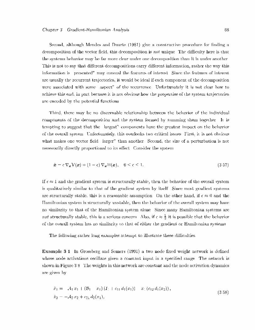
Chapter �� Gradient�Hamiltonian Analysis ��
Second� although Mendes and Duarte ������ give a constructive procedure for �nding a
decomposition of the vector �eld� this decomposition is not unique� The di�culty here is that
the systems behavior may be far more clear under one decomposition than it is under another�
This is not to say that di�erent decompositions carry di�erent information� rather the way this
information is �presented may conceal the features of interest� Since the features of interest
are usually the recurrent trajectories� it would be ideal if each component of the decomposition
were associated with some �aspect of the recurrence� Unfortunately it is not clear how to
achieve this end� in part because it is not obvious how the properties of the system trajectories
are encoded by the potential functions�
Third� there may be no discernable relationship between the behavior of the individual
components of the decomposition and the system formed by summing them together� It is
tempting to suggest that the �largest components have the greatest impact on the behavior
of the overall system� Unfortunately� this overlooks two critical issues� First� it is not obvious
what makes one vector �eld �larger than another� Second� the size of a perturbation is not
necessarily directly proportional to its e�ect� Consider the system
�x � rxV�x� � ��� �rxH�x�� � � � �� ������
If � � and the gradient system is structurally stable� then the behavior of the overall system
is qualitatively similar to that of the gradient system by itself� Since most gradient systems
are structurally stable� this is a reasonable assumption� On the other hand� if � � and the
Hamiltonian system is structurally unstable� then the behavior of the overall system may have
no similarity to that of the Hamiltonian system alone� Since many Hamiltonian systems are
not structurally stable� this is a serious concern� Also� if � �� it is possible that the behavior
of the overall system has no similarity to that of either the gradient or Hamiltonian systems�
The following rather long examples attempt to illustrate these di�culties�
Example ���� In Grossberg and Somers ������ a two node �xed weight network is de�ned
whose node activations oscillate given a constant input in a speci�ed range� The network is
shown in Figure ���� The weights in this network are constant and the node activation dynamics
are given by
�x� � �A� x� � �B� � x�� �I� � c�� d��x���� x� �c�� d��x��� �
�x� � �A� x� � c�� d��x���������
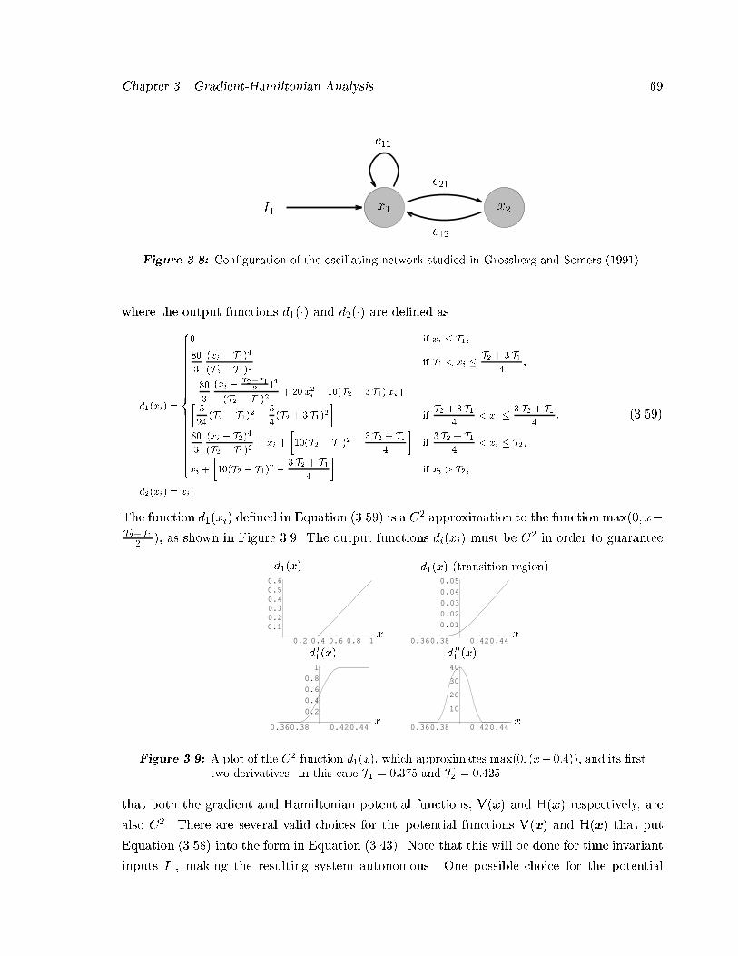
Chapter �� Gradient�Hamiltonian Analysis ��
c��
c��
c��
x�x�I�
Figure ��� Con�guration of the oscillating network studied in Grossberg and Somers � �� ��
where the output functions d���� and d���� are de�ned as
d��xi �
�����������������������������������������
� if xi � T���
�
�xi � T���T� � T��
if T� � xi � T� � � T��
���
�
�xi � T��T��
�
�T� � T��� �� x�i � ���T� � � T� xi��
�
���T� � T�� � �
��T� � � T��
�ifT� � � T�
�� xi � � T� � T�
�
��
�
�xi � T���T� � T��
� xi �
����T� � T�� � � T� � T�
�
�if
� T� � T��
� xi � T�
xi �
����T� � T�� � � T� � T�
�
�if xi � T�
d��xi � xi�
������
The function d��xi� de�ned in Equation ������ is a C� approximation to the function max��� x�T��T�
� �� as shown in Figure ���� The output functions di�xi� must be C� in order to guarantee
0.2 0.4 0.6 0.8 1
0.10.20.30.40.50.6
0.360.38 0.420.44
0.01
0.02
0.03
0.04
0.05
0.360.38 0.420.44
0.2
0.4
0.6
0.8
1
0.360.38 0.420.44
10
20
30
40
x
d��x�
x
d��x� �transition region�
x
d ���x�
x
d ��� �x�
Figure ���� A plot of the C� function d��x�� which approximates max��� �x� ������ and its �rsttwo derivatives� In this case T� ����� and T� ������
that both the gradient and Hamiltonian potential functions� V�x� and H�x� respectively� are
also C�� There are several valid choices for the potential functions V�x� and H�x� that put
Equation ������ into the form in Equation ������� Note that this will be done for time invariant
inputs I�� making the resulting system autonomous� One possible choice for the potential
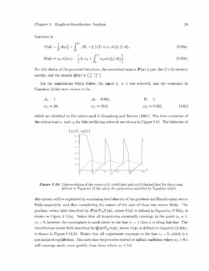
Chapter �� Gradient�Hamiltonian Analysis ��
functions is
V�x� ��
�A�x
�� �
Z x�
��B� � ��� �I� � c�� d������ d��� �����a�
H�x� � c�� d��x�� �
�A� x� �
Z x�
�c�� d����� d��
�� �����b�
For this choice of the potential functions� the associated matrix P �x� is just the �� �� identity
matrix� and the matrix Q�x� is�
� �x�x� �
��
For the simulations which follow� the input I� � � was selected� and the constants in
Equation ������ were chosen to be
A� � �� A� � ������ B� � ��
c�� � ��� c�� � ����� c�� � ������ ������
which are identical to the values used in Grossberg and Somers ������� The time evolution of
the activations x� and x� for this oscillating network are shown in Figure ����� The behavior of
20 40 60 80 100
0.4
0.5
0.6
0.7
0.8
0.9
t
fx��t�� x��t� g
Figure ����� Time evolution of the states x��t� �solid line� and x��t� �dashed line� for the systemde�ned in Equation ������ using the parameters speci�ed by Equation ���� ��
this system will be explained by examining the behavior of the gradient and Hamiltonian vector
�elds separately� and then considering the nature of the sum of these two vector �elds� The
gradient vector �eld described by P �x�rxV�x�� where V�x� is de�ned in Equation �����a�� is
shown in Figure �����a�� Notice that all trajectories eventually converge to the point x� � ��
x� � �� however the convergence is much faster to the line x� � � than it is along this line� The
Hamiltonian vector �eld described byQ�x�rxH�x�� where H�x� is de�ned in Equation �����b��
is shown in Figure �����b�� Notice that all trajectories converge to the line x� � �� which is a
non�isolated equilibrium� Also note that trajectories started at initial conditions where x� � ���
will converge much more quickly than those where x� � ����
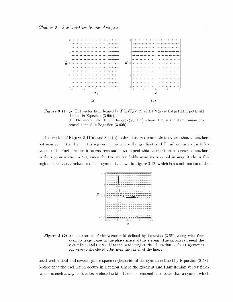
Chapter �� Gradient�Hamiltonian Analysis ��
-2 -1 0 1 2-2
-1
0
1
2
x�
x�
�a�
-2 -1 0 1 2-2
-1
0
1
2
x�
x�
�b�
Figure ����� �a� The vector �eld de�ned by P �x�rxV�x� where V�x� is the gradient potentialde�ned in Equation �����a���b� The vector �eld de�ned by Q�x�rxH�x� where H�x� is the Hamiltonian po�tential de�ned in Equation �����b��
Inspection of Figures �����a� and �����b� makes it seem reasonable to expect that somewhere
between x� � � and x� � � a region occurs where the gradient and Hamiltonian vector �elds
cancel out� Furthermore it seems reasonable to expect this cancelation to occur somewhere
in the region where x� � � since the two vector �elds seem more equal in magnitude in this
region� The actual behavior of this system is shown in Figure ����� which is a combination of the
-0.5 0 0.5 1 1.5-0.5
0
0.5
1
1.5
x�
x�
Figure ����� An illustration of the vector �eld de�ned by Equation ������� along with fourexample trajectories in the phase space of this system� The arrows represent thevector �eld� and the solid lines show the trajectories� Note that all four trajectoriesconverge to the closed orbit near the center of the �gure�
total vector �eld and several phase space trajectories of the system de�ned by Equation �������
Notice that the oscillation occurs in a region where the gradient and Hamiltonian vector �elds
cancel in such a way as to allow a closed orbit� It seems reasonable to state that a system which
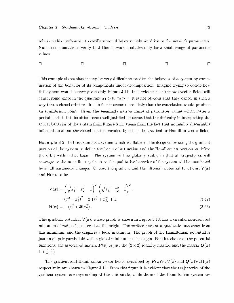
Chapter �� Gradient�Hamiltonian Analysis ��
relies on this mechanism to oscillate would be extremely sensitive to the network parameters�
Numerous simulations verify that this network oscillates only for a small range of parameter
values�
� � � � �
This example shows that it may be very di�cult to predict the behavior of a system by exam�
ination of the behavior of its components under decomposition� Imagine trying to decide how
this system would behave given only Figure ����� It is evident that the two vector �elds will
cancel somewhere in the quadrant x� � �� x� � �� It is not obvious that they cancel in such a
way that a closed orbit results� In fact it seems more likely that the cancelation would produce
an equilibrium point� Given the seemingly narrow range of parameter values which foster a
periodic orbit� this intuition seems well justi�ed� It seems that the di�culty in interpreting the
actual behavior of the system from Figure ����� stems from the fact that no readily discernable
information about the closed orbit is encoded by either the gradient or Hamilton vector �elds�
Example ���� In this example� a system which oscillates will be designed by using the gradient
portion of the system to de�ne the basin of attraction and the Hamiltonian portion to de�ne
the orbit within that basin� The system will be globally stable in that all trajectories will
converge to the same limit cycle� Also the qualitative behavior of the system will be una�ected
by small parameter changes� Choose the gradient and Hamiltonian potential functions� V�x�
and H�x�� to be
V�x� �
�qx�� � x�� � �
�� �qx�� � x�� � �
��
�
��x�� � x��
�� � ��x�� � x��
�� �� ������
H�x� � � �x�� � ��x���� ������
This gradient potential V�x�� whose graph is shown in Figure ����� has a circular non�isolated
minimum of radius �� centered at the origin� The surface rises at a quadratic rate away from
this minimum� and the origin is a local maximum� The graph of the Hamiltonian potential is
just an elliptic paraboloid with a global minimum at the origin� For this choice of the potential
functions� the associated matrix P �x� is just the �� �� identity matrix� and the matrix Q�x�
is�
� ��� �
��
The gradient and Hamiltonian vector �elds� described by P �x�rxV�x� and Q�x�rxH�x�
respectively� are shown in Figure ����� From this �gure it is evident that the trajectories of the
gradient system are rays ending at the unit circle� while those of the Hamiltonian system are
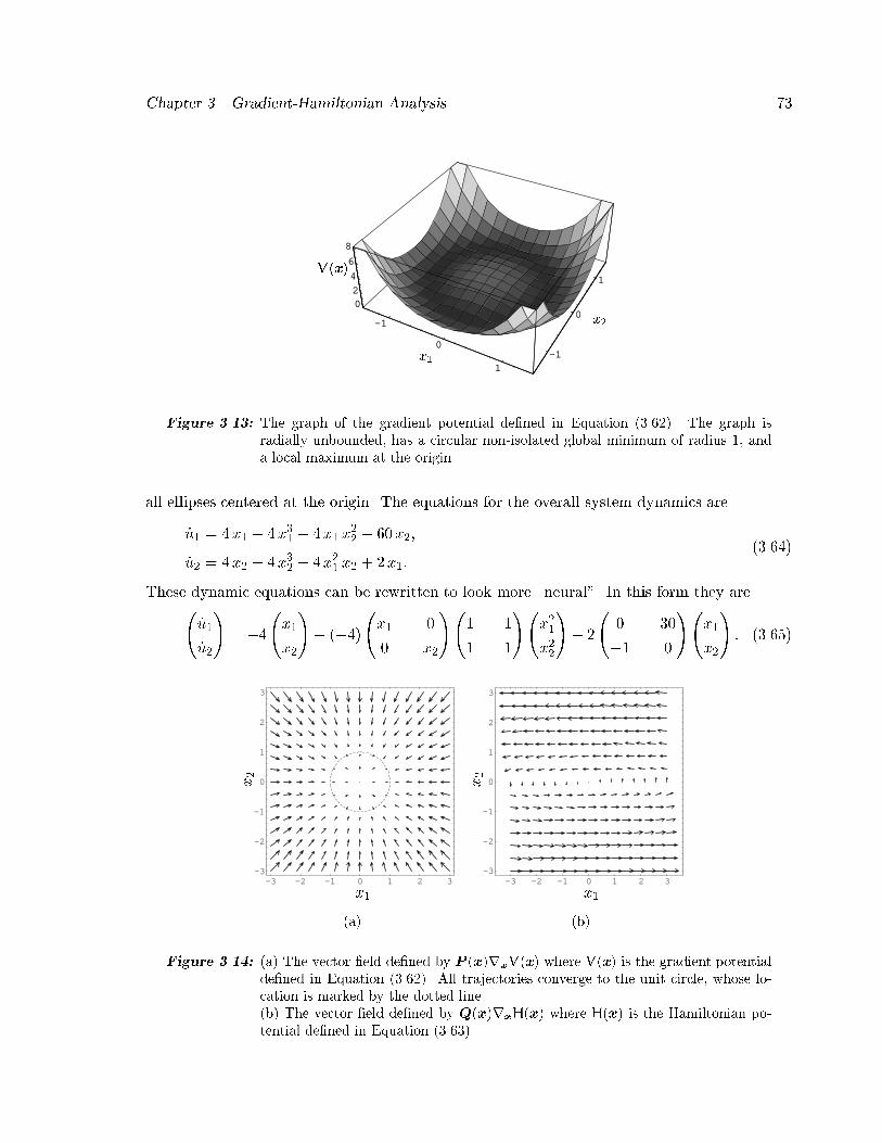
Chapter �� Gradient�Hamiltonian Analysis ��
-1
0
1-1
0
1
02
4
6
8
-1
0
1-1
0
1
02
4
6
8
x�
x�
V�x�
x�
x�
V�x�
Figure ����� The graph of the gradient potential de�ned in Equation ������� The graph isradially unbounded� has a circular non�isolated global minimum of radius � anda local maximum at the origin�
all ellipses centered at the origin� The equations for the overall system dynamics are
�u� � �x� � �x�� � �x� x�� � ��x��
�u� � �x� � �x�� � �x�� x� � �x��������
These dynamic equations can be rewritten to look more �neural� In this form they are��u�
�u�
�� ��
�x�
x�
�� ����
�x� �
� x�
��� �
� �
��x��
x��
�� �
�� ��
�� �
��x�
x�
�� ������
-3 -2 -1 0 1 2 3-3
-2
-1
0
1
2
3
x�
x�
�a�
-3 -2 -1 0 1 2 3-3
-2
-1
0
1
2
3
x�
x�
�b�
Figure ����� �a� The vector �eld de�ned by P �x�rxV�x� where V�x� is the gradient potentialde�ned in Equation ������� All trajectories converge to the unit circle� whose lo�cation is marked by the dotted line��b� The vector �eld de�ned by Q�x�rxH�x� where H�x� is the Hamiltonian po�tential de�ned in Equation �������
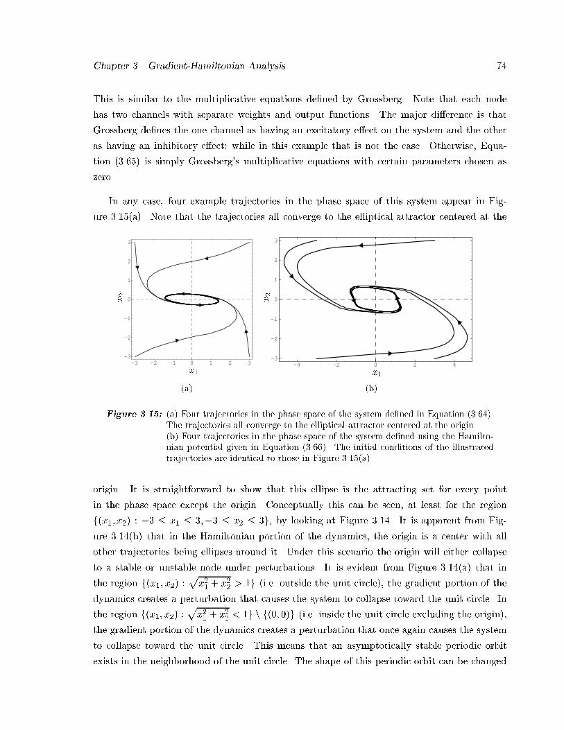
Chapter �� Gradient�Hamiltonian Analysis ��
This is similar to the multiplicative equations de�ned by Grossberg� Note that each node
has two channels with separate weights and output functions� The major di�erence is that
Grossberg de�nes the one channel as having an excitatory e�ect on the system and the other
as having an inhibitory e�ect� while in this example that is not the case� Otherwise� Equa�
tion ������ is simply Grossbergs multiplicative equations with certain parameters chosen as
zero�
In any case� four example trajectories in the phase space of this system appear in Fig�
ure �����a�� Note that the trajectories all converge to the elliptical attractor centered at the
-3 -2 -1 0 1 2 3-3
-2
-1
0
1
2
3
x�
x�
�a�
-4 -2 0 2 4-3
-2
-1
0
1
2
3
x�
x�
�b�
Figure ����� �a� Four trajectories in the phase space of the system de�ned in Equation �������The trajectories all converge to the elliptical attractor centered at the origin��b� Four trajectories in the phase space of the system de�ned using the Hamilto�nian potential given in Equation ������� The initial conditions of the illustratedtrajectories are identical to those in Figure �� ��a��
origin� It is straightforward to show that this ellipse is the attracting set for every point
in the phase space except the origin� Conceptually this can be seen� at least for the region
f�x�� x�� � �� � x� � ���� � x� � �g� by looking at Figure ����� It is apparent from Fig�
ure �����b� that in the Hamiltonian portion of the dynamics� the origin is a center with all
other trajectories being ellipses around it� Under this scenario the origin will either collapse
to a stable or unstable node under perturbations� It is evident from Figure �����a� that in
the region f�x�� x�� �px�� � x�� � �g �i�e� outside the unit circle�� the gradient portion of the
dynamics creates a perturbation that causes the system to collapse toward the unit circle� In
the region f�x�� x�� �px�� � x�� � �g n f��� ��g �i�e� inside the unit circle excluding the origin��
the gradient portion of the dynamics creates a perturbation that once again causes the system
to collapse toward the unit circle� This means that an asymptotically stable periodic orbit
exists in the neighborhood of the unit circle� The shape of this periodic orbit can be changed
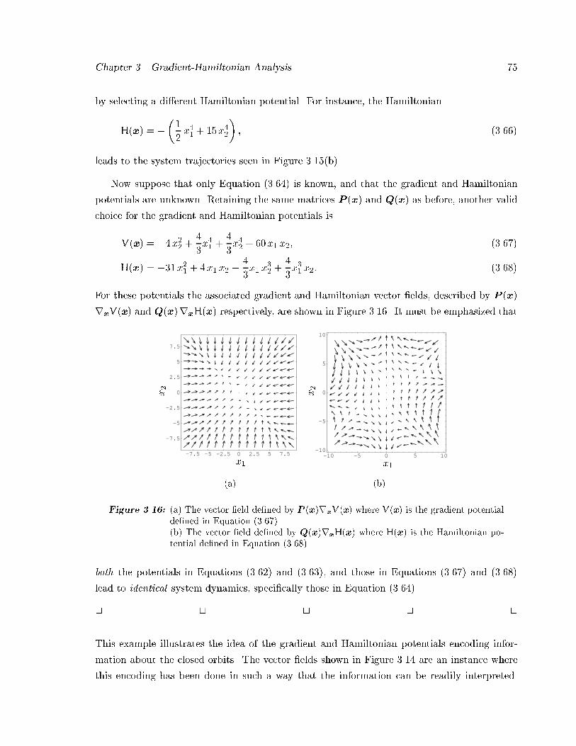
Chapter �� Gradient�Hamiltonian Analysis ��
by selecting a di�erent Hamiltonian potential� For instance� the Hamiltonian
H�x� � ���
�x�� � ��x��
�� ������
leads to the system trajectories seen in Figure �����b��
Now suppose that only Equation ������ is known� and that the gradient and Hamiltonian
potentials are unknown� Retaining the same matrices P �x� and Q�x� as before� another valid
choice for the gradient and Hamiltonian potentials is
V�x� � ��x�� ��
�x�� �
�
�x�� � ��x� x�� ������
H�x� � ���x�� � �x� x� � �
�x� x
�� �
�
�x�� x�� ������
For these potentials the associated gradient and Hamiltonian vector �elds� described by P �x�
rxV�x� and Q�x�rxH�x� respectively� are shown in Figure ����� It must be emphasized that
-7.5 -5 -2.5 0 2.5 5 7.5
-7.5
-5
-2.5
0
2.5
5
7.5
x�
x�
�a�
-10 -5 0 5 10-10
-5
0
5
10
x�
x�
�b�
Figure ����� �a� The vector �eld de�ned by P �x�rxV�x� where V�x� is the gradient potentialde�ned in Equation ��������b� The vector �eld de�ned by Q�x�rxH�x� where H�x� is the Hamiltonian po�tential de�ned in Equation �������
both the potentials in Equations ������ and ������� and those in Equations ������ and ������
lead to identical system dynamics� speci�cally those in Equation �������
� � � � �
This example illustrates the idea of the gradient and Hamiltonian potentials encoding infor�
mation about the closed orbits� The vector �elds shown in Figure ���� are an instance where
this encoding has been done in such a way that the information can be readily interpreted�

Chapter �� Gradient�Hamiltonian Analysis ��
Conversely� the vector �elds in Figure ���� are an instance where this information is not read�
ily available� In short� unless the three issues discussed at the beginning of the section can
be resolved� it is di�cult to see how to use this decomposition to e�ectively analyze a given
dynamical system� Example ��� suggests that the intuition about the behavior of gradient
and Hamiltonian systems may be a very useful tool for designing systems with certain desired
properties� This will be discussed in the next chapter�
In this chapter it has been shown that the dynamics of many existing neural network archi�
tectures can be decomposed into the sum of a gradient�like term and a Hamiltonian�like term�
An attempt was made to use this result to analyze the dynamics of existing neural networks�
While this was done successfully in some cases� it was pointed out that there are unresolved
di�culties which prevent a general analysis at this time� In the next chapter the the comple�
mentary characteristics of gradient and Hamiltonian systems will be used to synthesize a class
of nonlinear models for system identi�cation� A learning algorithm will be proposed� which
under certain model restrictions� will be proven to converge to a set of parameters for which
the error between the model output and that of the actual system vanishes�
Chapter �
Gradient�Hamiltonian Synthesis
Another way to make use of the gradient and Hamiltonian systems is to use the intuitive
understanding of their behavior to synthesize systems which have some desired qualitative
behavior� For instance� gradient systems can be used to represent the convergent properties
of a system� and Hamiltonian systems can be used to represent the periodic properties� The
central idea of this chapter is to use gradient�like and Hamiltonian�like systems to construct
a class of models for system identi�cation� In Section ��� the class of parametrized models
proposed by Cohen ������ are reviewed� These models are classes of parametrized ordinary
di�erential equations� These models possess the following three properties� First� the prescribed
set of equilibria are guaranteed to be the only equilibria of the model� no spurious equilibria
are possible� Second� these equilibria are globally stable in that all initial values will lead to
one of the prescribed equilibria� Third� the equilibria remain the same under perturbation of
certain parameter values� In Cohen ������ no method is proposed for learning the parameter
values from example data� In Section ��� these models are extended for system identi�cation
by introducing an appropriate input term� In the process it is shown that the models in Cohen
������ are a subset of the gradient�Hamiltonian systems discussed in Mendes and Duarte �������
Furthermore� given certain restrictions in the parametrization� a learning rule is introduced for
these identi�cation models which is proven to converge to a set of parameters which guarantee
that the error between the output of the actual system and that of the model vanishes� In
Section ��� a simple example of these models is simulated and the results discussed� Lastly� in
Section ��� these models are assessed in the framework proposed by Sj!oberg ������ for general
identi�cation models�

Chapter �� Gradient�Hamiltonian Synthesis ��
��� Review of Cohen�s Model
The major result of Cohen ������ is to propose two constructions for a class of parametrized
di�erential equations for modeling systems� The constructions assume that the equilibria of the
desired system are known� This being the case both constructions give a system of parametrized
di�erential equations which possess the desired equilibria for all choices of the parameter val�
ues� The purpose of the parameters is to determine the manner in which the equilibria are
approached� One important feature of these constructions is that they produce di�erential
equations whose only equilibria are the desired ones� Furthermore� the desired equilibria are
globally stable in that all initial values evolve to one of the desired equilibria�
The �rst construction deals with the case where all of the equilibria are points� speci�cally
either point attractors or saddle points� Conceptually this construction projects the entire sys�
tem dynamics onto one dimension of the system� without loss of generality� the �rst dimension
can always be chosen� This means that in the �rst dimension the system always converges to
the �rst coordinate value of one of the equilibrium points� Each additional coordinate value
�i�e� second� third� etc�� of an equilibrium point is interpolated from the �rst coordinate using
a Lagrange interpolation polynomial� The dynamics� in all coordinates except the �rst� ex�
ponentially decay to these interpolated values� This construction� discussed in Theorem � of
Cohen ������� is schematized for a ��dimensional example in Figure ���� First choose a set of
points A� whose coordinates de�ne the locations of the desired point attractors� these points
will be local minima of the potential function� In Figure ��� these are the two points labeled
�� and ��� Project each of these points onto the x� coordinate axis� Then choose a second set
of points R which will be the saddle points of the potential function� The x� coordinate value
of each point in R must lie in between the x� coordinate values of two adjacent points from A�
In Figure ��� this is the one point labeled ��� Now construct a polynomial function of x� which
vanishes at the x� coordinate values of all of the points in both A and R� This is the polynomial
labeled �L��x�� in Figure ���� For each of the other coordinates xi� i � �� � � � �n� construct
a Lagrange interpolation polynomial Li�x�� such that the value of this polynomial at the x�
coordinate of any point in A or R is the projection of that point onto the xi coordinate axis�
The dynamics of this system in the x� direction are merely given by the polynomial �L��x���In the other directions� the system exponentially decays to the value of Li�x�� corresponding
to the value of x�� The speci�cs of this construction are given by Theorem � in Cohen �������
which is paraphrased below� In the theorem� xi��j� denotes the ith coordinate of the jth point
�j� For example� if �� � ��� �� �� �� then x����� � �� because � is the second element of ���
Theorem ��� �Cohen Theorem � � Let f��� ��� � � � � �eg be a set of e given points in Rn
such that a� � x����� � a� � x����� � � � � � ae � x���e�� Choose an arbitrary set of e � �
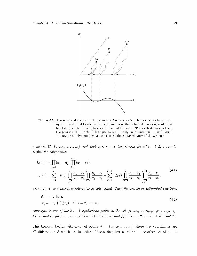
Chapter �� Gradient�Hamiltonian Synthesis ��
x�x�
x�
x�
��
�L��x��
�
�
Figure ���� The scheme described in Theorem � of Cohen � ����� The points labeled � and� are the desired locations for local minima of the potential function� while thatlabeled �� is the desired location for a saddle point� The dashed lines indicatethe projections of each of these points onto the x� coordinate axis� The function�L��x�� is a polynomial which vanishes at the x� coordinates of the � points�
points in Rn f��� ��� � � � � �e��g such that ai � ri � x���i� � ai�� for all i � �� �� � � � � e � ��
De�ne the polynomials
L��x�� �eY
j��
�x� � aj�e��Yk��
�x� � rk��
Li�x�� �eX
j��
xi��j�eY
s��s�j
x� � as
aj � as
e��Yt��
x� � rt
aj � rt�e��Xk��
xi��k�eY
u��
x� � au
rk � au
e��Yv��v �k
x� � rv
rk � rv�
�����
where Li�x�� is a Lagrange interpolation polynomial� Then the system of di�erential equations
�x� � �L��x����xi � �xi � Li�x�� � i � �� � � � �n�
�����
converges to one of the � e � � equilibrium points in the set f��� ��� � � � � �e� ��� ��� � � � � �e��g�Each point �i for i � �� �� � � � � e is a sink� and each point �i for i � �� �� � � � � e� � is a saddle�
This theorem begins with a set of points A � f��� ��� � � � � �eg whose �rst coordinates are
all di�erent� and which are in order of increasing �rst coordinate� Another set of points
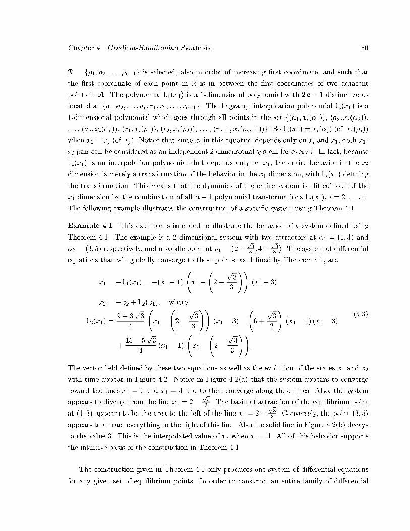
Chapter �� Gradient�Hamiltonian Synthesis ��
R � f��� ��� � � � � �e��g is selected� also in order of increasing �rst coordinate� and such that
the �rst coordinate of each point in R is in between the �rst coordinates of two adjacent
points in A� The polynomial L��x�� is a ��dimensional polynomial with � e � � distinct zeros
located at fa�� a�� � � � � ae� r�� r�� � � � � re��g� The Lagrange interpolation polynomial Li�x�� is a
��dimensional polynomial which goes through all points in the set f�a�� xi������ �a�� xi������
� � � � �ae� xi��e��� �r�� xi������ �r�� xi������ � � � � �re��� xi��m����g� So Li�x�� � xi��j� �cf� xi��j��
when x� � aj �cf� rj�� Notice that since �xi in this equation depends only on xi and x�� each �x��
�xi pair can be considered as an independent ��dimensional system for every i� In fact� because
Li�x�� is an interpolation polynomial that depends only on x�� the entire behavior in the xi
dimension is merely a transformation of the behavior in the x� dimension� with Li�x�� de�ning
the transformation� This means that the dynamics of the entire system is �lifted out of the
x� dimension by the combination of all n� � polynomial transformations Li�x��� i � �� � � � �n�
The following example illustrates the construction of a speci�c system using Theorem ����
Example ���� This example is intended to illustrate the behavior of a system de�ned using
Theorem ���� The example is a ��dimensional system with two attractors at �� � ��� �� and
�� � ��� �� respectively� and a saddle point at �� � ���p�� � ��
p�� �� The system of di�erential
equations that will globally converge to these points� as de�ned by Theorem ���� are
�x� � �L��x�� � ��x� � ��
�x� �
���
p�
�
���x� � ���
�x� � �x� � L��x��� where
L��x�� �� � �
p�
�
�x� �
���
p�
�
���x� � ���
�� �
p�
�
��x� � �� �x� � ��
���� �
p�
��x� � ��
�x� �
���
p�
�
���
�����
The vector �eld de�ned by these two equations as well as the evolution of the states x� and x�
with time appear in Figure ���� Notice in Figure ����a� that the system appears to converge
toward the lines x� � � and x� � � and to then converge along these lines� Also� the system
appears to diverge from the line x� � ��p�� � The basin of attraction of the equilibrium point
at ��� �� appears to be the area to the left of the line x� � ��p�� � Conversely� the point ��� ��
appears to attract everything to the right of this line� Also the solid line in Figure ����b� decays
to the value �� This is the interpolated value of x� when x� � �� All of this behavior supports
the intuitive basis of the construction in Theorem ����
The construction given in Theorem ��� only produces one system of di�erential equations
for any given set of equilibrium points� In order to construct an entire family of di�erential
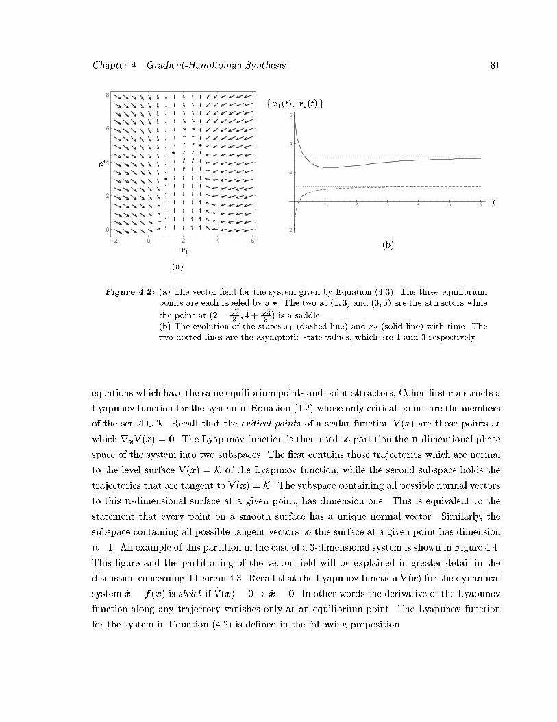
Chapter �� Gradient�Hamiltonian Synthesis ��
-2 0 2 4 6
0
2
4
6
8
x�
x�
�a�
1 2 3 4 5 6
-2
2
4
6
t
fx��t�� x��t� g
�b�
Figure ���� �a� The vector �eld for the system given by Equation ������ The three equilibriumpoints are each labeled by a �� The two at � � �� and ��� �� are the attractors while
the point at ���p�� � � �
p�� � is a saddle�
�b� The evolution of the states x� �dashed line� and x� �solid line� with time� Thetwo dotted lines are the asymptotic state values� which are and � respectively�
equations which have the same equilibrium points and point attractors� Cohen �rst constructs a
Lyapunov function for the system in Equation ����� whose only critical points are the members
of the set A � R� Recall that the critical points of a scalar function V�x� are those points at
which rxV�x� � � The Lyapunov function is then used to partition the n�dimensional phase
space of the system into two subspaces� The �rst contains those trajectories which are normal
to the level surface V�x� � K of the Lyapunov function� while the second subspace holds the
trajectories that are tangent to V�x� � K� The subspace containing all possible normal vectors
to this n�dimensional surface at a given point� has dimension one� This is equivalent to the
statement that every point on a smooth surface has a unique normal vector� Similarly� the
subspace containing all possible tangent vectors to this surface at a given point has dimension
n��� An example of this partition in the case of a ��dimensional system is shown in Figure ����
This �gure and the partitioning of the vector �eld will be explained in greater detail in the
discussion concerning Theorem ���� Recall that the Lyapunov function V�x� for the dynamical
system �x � f�x� is strict if �V�x� � �� �x � � In other words the derivative of the Lyapunov
function along any trajectory vanishes only at an equilibrium point� The Lyapunov function
for the system in Equation ����� is de�ned in the following proposition�
Chapter �� Gradient�Hamiltonian Synthesis ��
Theorem ��� �Cohen Proposition � � For all C � �� the function
V�x� � CZ x�
X�L���� d� �
nXi��
��
��xi � Li�x���
� ��
�
Z x�
XiL����
�L�i���
��d�
�� �����
is a strict Lyapunov function for the system of Equation ����� with time derivative
�V�x� �C �L��x���� �nXi��
��xi � Li�x����
�L��x�� L�i�x��
�
�
��L��x���� �L�i�x���
�
������
where C is a real positive constant� Xi � i � �� � � � �n are real constants chosen so that the
integrals are positive valued� and L�i�x�� � dLidx�
�
Example ���� This example illustrates the properties of a system whose dynamics are de�ned
as vectors normal to the Lyapunov function V�x� de�ned in Equation ������ The di�erential
equations of motion for such a system are �x � �rxV�x�� The starting point is the system
discussed in Example ���� so the polynomials L��x�� and L��x�� are those de�ned in Equa�
tion ������ The Lyapunov function for this example� choosing C � � is
V�x�� x�� � �
Z x�
�L���� d� �
�
��x� � L��x���
� ��
�
Z x�
�L����
�L�����
��d�� where
L���x�� � �� � �p�
��x� � �� �
���
p�
�
��x� �
���
p�
�
��� ���p�
��x� � ��
�����
With this Lyapunov function the dynamic equations are
�x� � � �V
�x�� �L��x��
�� �
�
��L���x���
�
�� L���x�� �x� � L��x��� �
�x� � � �V
�x�� �x� � L��x���
�����
Notice that only the dynamics in the x� dimension of the phase space have changed from those
in Equation ������ Due to the form of the Lyapunov function V�x� in Equation ������ this will
be true for any system de�ned by �x � �rxV�x� regardless of the number of dimensions� The
vector �eld de�ned by these two equations as well as the evolution of the states x� and x� with
time appear in Figure ���� Notice that this �gure is very similar to Figure ��� in that the system
still converges globally to one of the three points in the set f��� ��� ��� ��� ���p�� � ��
p�� �g� One
di�erence between the two �gures is that in Figure ����a� the equilibrium points are no longer
approached in the x� direction along the lines x� � �� x� � � �p�� � and x� � �� Instead� the
change in the x� dynamics has twisted these lines into S�shaped curves� The basin of attraction
for the point ��� �� now appears to be a square region to the left of the line x� � � and below
the line x� � �� The remainder of the space is attracted to ��� ��� Also� in Figure ����b� the
initial condition which converged to the point ��� �� in Figure ����b�� now converges to the
point ��� ���
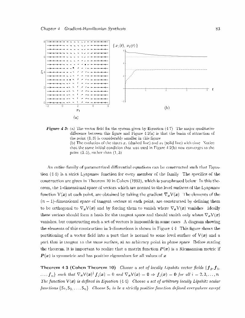
Chapter �� Gradient�Hamiltonian Synthesis ��
-2 0 2 4 60
2
4
6
8
x�
x�
�a�
1 2 3 4
-2
2
4
6
t
fx��t�� x��t� g
�b�
Figure ���� �a� The vector �eld for the system given by Equation ������ The major qualitativedi�erence between this �gure and Figure ����a� is that the basin of attraction ofthe point � � �� is considerably smaller in this �gure��b� The evolution of the states x� �dashed line� and x� �solid line� with time� Noticethat the same initial condition that was used in Figure ����b� now converges to thepoint ��� ��� rather than � � ���
An entire family of parametrized di�erential equations can be constructed such that Equa�
tion ����� is a strict Lyapunov function for every member of the family� The speci�cs of the
construction are given in Theorem �� in Cohen ������� which is paraphrased below� In this the�
orem� the ��dimensional space of vectors which are normal to the level surfaces of the Lyapunov
function V�x� at each point� are obtained by taking the gradient rxV�x�� The elements of the
�n � ���dimensional space of tangent vectors at each point� are constructed by de�ning them
to be orthogonal to rxV�x� and by forcing them to vanish where rxV�x� vanishes� Ideally
these vectors should form a basis for the tangent space and should vanish only where rxV�x�
vanishes� but constructing such a set of vectors is impossible in some cases� A diagram showing
the elements of this construction in ��dimensions is shown in Figure ���� This �gure shows the
partitioning of a vector �eld into a part that is normal to some level surface of V�x� and a
part that is tangent to the same surface� at an arbitrary point in phase space� Before stating
the theorem� it is important to realize that a matrix function P �x� is a Riemannian metric if
P �x� is symmetric and has positive eigenvalues for all values of x�
Theorem ��� �Cohen Theorem � � Choose a set of locally Lipshitz vector �elds ff ��f��
� � � �fng such that rxV�x�y f i�x� � � and rxV�x� � � f i�x� � for all i � �� �� � � � �n�
The function V�x� is de�ned in Equation ������ Choose a set of arbitrary locally Lipshitz scalar
functions fS��S�� � � � �Sng� Choose S� to be a strictly positive function de�ned everywhere except
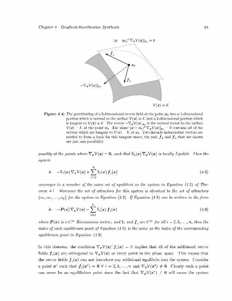
Chapter �� Gradient�Hamiltonian Synthesis ��
V�x� K
x�
f �
�x� x��yrxV�x�jx� �
f �
�rxV�x�jx�
Figure ���� The partitioning of a ��dimensional vector �eld at the point x� into a �dimensionalportion which is normal to the surface V�x� K and a ��dimensional portion whichis tangent to V�x� K� The vector �rxV�x�jx� is the normal vector to the surfaceV�x� K at the point x�� The plane �x� x��yrxV�x�jx� � contains all of thevectors which are tangent to V�x� K at x�� Two linearly independent vectors areneeded to form a basis for this tangent space� the pair f� and f� that are shownare just one possibility�
possibly at the points where rxV�x� � � such that S��x�rxV�x� is locally Lipshitz� Then the
system
�x � �S��x�rxV�x� �nXi��
Si�x�f i�x� �����
converges to a member of the same set of equilibria as the system in Equation ����� of The�
orem ���� Moreover the set of attractors for this system is identical to the set of attractors
f��� ��� � � � � �eg for the system in Equation ������ If Equation ����� can be written in the form
�x � �P �x�rxV�x� �
nXi��
Si�x�f i�x� �����
where P �x� is a C� Riemannian metric� and Si and f i are C� for all i � �� �� � � � �n� then the
index of each equilibrium point of Equation ����� is the same as the index of the corresponding
equilibrium point in Equation ������
In this theorem� the condition rxV�x�y f i�x� � � implies that all of the additional vector
�elds f i�x� are orthogonal to rxV�x� at every point in the phase space� This means that
the vector �elds f i�x� can not introduce any additional equilibria into the system� Consider
a point x� such that f i�x�� � � i � �� �� � � � �n and rxV�x�� �� � Clearly such a point
can never be an equilibrium point since the fact that rxV�x�� �� will cause the system
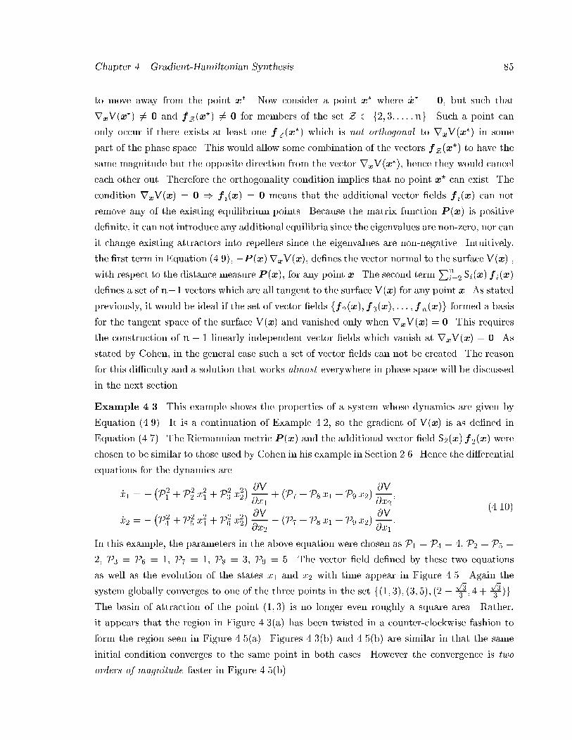
Chapter �� Gradient�Hamiltonian Synthesis ��
to move away from the point x�� Now consider a point x where �x � � but such that
rxV�x � �� and fZ�x � �� for members of the set Z f�� �� � � � �ng� Such a point can
only occur if there exists at least one fZ�x � which is not orthogonal to rxV�x � in some
part of the phase space� This would allow some combination of the vectors fZ�x � to have the
same magnitude but the opposite direction from the vector rxV�x �� hence they would cancel
each other out� Therefore the orthogonality condition implies that no point x can exist� The
condition rxV�x� � � f i�x� � means that the additional vector �elds f i�x� can not
remove any of the existing equilibrium points� Because the matrix function P �x� is positive
de�nite� it can not introduce any additional equilibria since the eigenvalues are non�zero� nor can
it change existing attractors into repellers since the eigenvalues are non�negative� Intuitively�
the �rst term in Equation ������ �P �x�rxV�x�� de�nes the vector normal to the surface V�x� �
with respect to the distance measure P �x�� for any point x� The second termPn
i�� Si�x�f i�x�
de�nes a set of n�� vectors which are all tangent to the surface V�x� for any point x� As stated
previously� it would be ideal if the set of vector �elds ff��x��f��x�� � � � �fn�x�g formed a basis
for the tangent space of the surface V�x� and vanished only when rxV�x� � � This requires
the construction of n � � linearly independent vector �elds which vanish at rxV�x� � � As
stated by Cohen� in the general case such a set of vector �elds can not be created� The reason
for this di�culty and a solution that works almost everywhere in phase space will be discussed
in the next section�
Example ���� This example shows the properties of a system whose dynamics are given by
Equation ������ It is a continuation of Example ���� so the gradient of V�x� is as de�ned in
Equation ������ The Riemannian metric P �x� and the additional vector �eld S��x�f��x� were
chosen to be similar to those used by Cohen in his example in Section ���� Hence the di�erential
equations for the dynamics are
�x� � � �P�� � P�
� x�� � P�
� x��
� �V
�x�� �P� � P� x� � P� x��
�V
�x��
�x� � � �P�� � P�
� x�� � P�
� x��
� �V
�x�� �P� � P� x� � P� x��
�V
�x��
������
In this example� the parameters in the above equation were chosen as P� � P� � �� P� � P� �
�� P� � P� � �� P� � �� P� � �� P� � �� The vector �eld de�ned by these two equations
as well as the evolution of the states x� and x� with time appear in Figure ���� Again the
system globally converges to one of the three points in the set f��� ��� ��� ��� �� �p�� � � �
p�� �g�
The basin of attraction of the point ��� �� is no longer even roughly a square area� Rather�
it appears that the region in Figure ����a� has been twisted in a counter�clockwise fashion to
form the region seen in Figure ����a�� Figures ����b� and ����b� are similar in that the same
initial condition converges to the same point in both cases� However the convergence is two
orders of magnitude faster in Figure ����b��
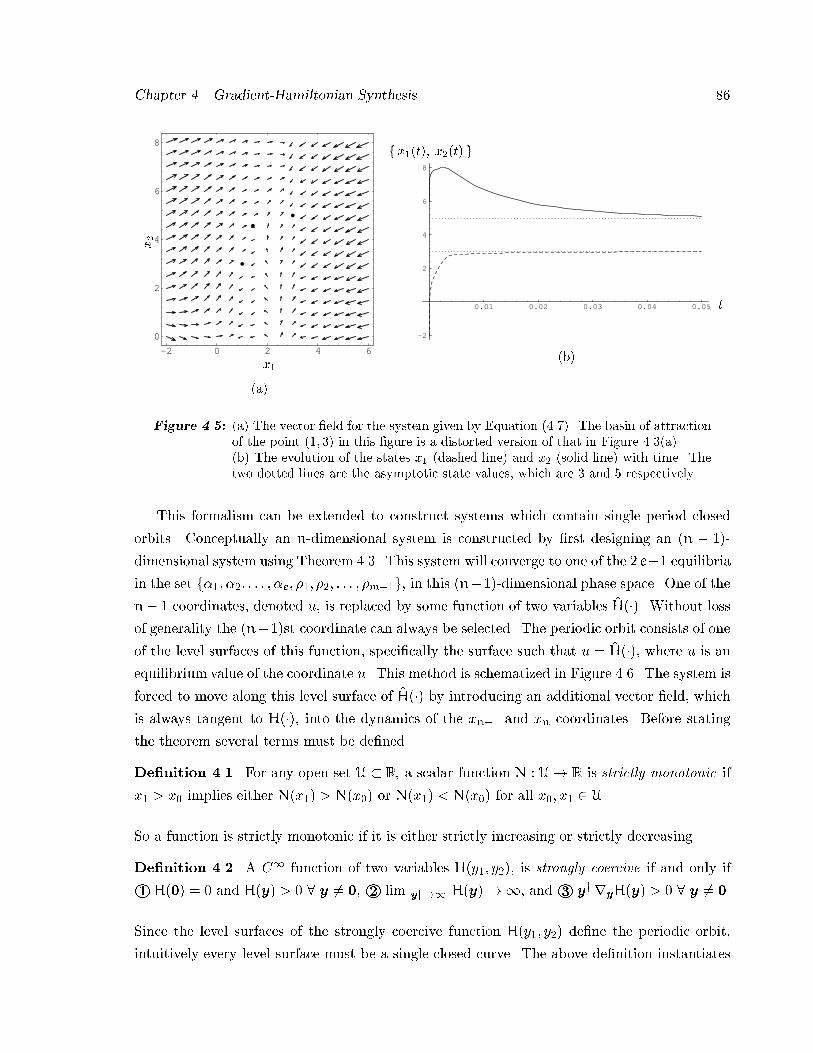
Chapter �� Gradient�Hamiltonian Synthesis ��
-2 0 2 4 6
0
2
4
6
8
x�
x�
�a�
0.01 0.02 0.03 0.04 0.05
-2
2
4
6
8
t
fx��t�� x��t� g
�b�
Figure ���� �a� The vector �eld for the system given by Equation ������ The basin of attractionof the point � � �� in this �gure is a distorted version of that in Figure ����a���b� The evolution of the states x� �dashed line� and x� �solid line� with time� Thetwo dotted lines are the asymptotic state values� which are � and � respectively�
This formalism can be extended to construct systems which contain single period closed
orbits� Conceptually an n�dimensional system is constructed by �rst designing an �n � ���
dimensional system using Theorem ���� This system will converge to one of the � e�� equilibria
in the set f��� ��� � � � � �e� ��� ��� � � � � �m��g� in this �n����dimensional phase space� One of the
n� � coordinates� denoted u� is replaced by some function of two variables H���� Without loss
of generality the �n���st coordinate can always be selected� The periodic orbit consists of one
of the level surfaces of this function� speci�cally the surface such that �u � H���� where �u is an
equilibrium value of the coordinate u� This method is schematized in Figure ���� The system is
forced to move along this level surface of H��� by introducing an additional vector �eld� which
is always tangent to H���� into the dynamics of the xn�� and xn coordinates� Before stating
the theorem several terms must be de�ned�
Denition ���� For any open set U R� a scalar function N � U� R is strictly monotonic if
x� � x� implies either N�x�� � N�x�� or N�x�� � N�x�� for all x�� x� � U�
So a function is strictly monotonic if it is either strictly increasing or strictly decreasing�
Denition ���� A C� function of two variables H�y�� y��� is strongly coercive if and only if
�� H�� � � and H�y� � � � y �� ��� limkyk�� H�y���� and�� yyryH�y� � � � y �� �
Since the level surfaces of the strongly coercive function H�y�� y�� de�ne the periodic orbit�
intuitively every level surface must be a single closed curve� The above de�nition instantiates
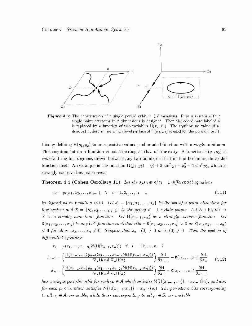
Chapter �� Gradient�Hamiltonian Synthesis ��
x�
�uu
x�
x�
x�
� �x��x�
�u �H�x�� x��
Figure ���� The construction of a single period orbit in � dimensions� First a system with asingle point attractor in � dimensions is designed� Then the coordinate labeled u
is replaced by a function of two variables �H�x�� x��� The equilibrium value of u�
denoted �u� determines which level surface of �H�x�� x�� is used for the periodic orbit�
this by de�ning H�y�� y�� to be a positive valued� unbounded function with a single minimum�
This requirement on a function is not as strong as that of convexity� A function H�y�� y�� is
convex if the line segment drawn between any two points on the function lies on or above the
function itself� An example is the function H�y�� y�� � y�� � � sin� y� � y�� � � sin� y�� which is
strongly coercive but not convex�
Theorem ��� �Cohen Corollary �� � Let the system of n� � di�erential equations
�xi � gi�x�� x�� � � � � xn��� � i � �� �� � � � �n� � ������
be de�ned as in Equation ������ Let A � f��� ��� � � � � �eg be the set of e point attractors for
this system and R � f��� ��� � � � � �e��g be the set of e � � saddle points� Let N � ����� �R be a strictly monotonic function� Let H�xn��� xn� be a strongly coercive function� Let
R�x�� x�� � � � � xn� be any C� function such that either R�x�� x�� � � � � xn� � � or R�x�� x�� � � � � xn�
� � for all x�� x�� � � � � xn �� �� Suppose that xn����� �� � or xn��� �� �� Then the system of
di�erential equations
�xi gi�x�� � � � � xn���N�H�xn��� xn��� � i � �� � � � �n� �
�xn��
�H�xn��� xn� gn���x�� � � � � xn���N�H�xn��� xn���
rxH�x�yrxH�x�
�H
�xn��� R�x�� � � � � xn�
�H
�xn
�xn
�H�xn��� xn� gn���x�� � � � � xn���N�H�xn��� xn���
rxH�x�yrxH�x�
�H
�xn� R�x�� � � � � xn�
�H
�xn��
������
has a unique periodic orbit for each �i � A which satis�es N�H�xn��� xn�� � xn����i�� and also
for each �i � R which satis�es N�H�xn��� xn�� � xn����i�� The periodic orbits corresponding
to all �i � A are stable� while those corresponding to all �i � R are unstable�
Chapter �� Gradient�Hamiltonian Synthesis ��
Conceptually� the periodic orbit de�ned by Equation ������ consists of one of the level sur�
faces of H�xn��� xn�� The level surface traversed by the system is determined by the con�
dition H�xn��� xn� � N���xn����j�� �cf� N���xn����j��� So the value of the �n � ��st co�
ordinate of each equilibrium point determines along which level surface of H�xn��� xn� the
corresponding periodic orbit moves� Every periodic orbit in this construction is constrained
to lie on a ��dimensional plane parallel to the xn�� and xn axes and passing through either
the point �x���j�� x���j�� � � � � xn����j�� �� �� or �x���j�� x���j�� � � � � xn����j�� �� ��� The terms
�R�x�� � � � � xn� �H�xn
and R�x�� � � � � xn��H
�xn��in Equation ������ de�ne a Hamiltonian vector �eld
which is always tangent to the level surfaces of H�xn��� xn�� These terms cause the system
to move along the level surfaces in a periodic manner� The function R�x�� x�� � � � � xn� acts as
a position dependent scaling factor� This function allows the velocity along the periodic orbit
to be controlled� For instance� two periodic orbits which have the same shape� H�xn��� xn� �
N���xn����j�� � N���xn����k�� for j �� k� will have di�erent velocities along the orbit if
R�x���j�� x���j�� � � � � xn����j�� xn��� xn� �� R�x���k�� x���k�� � � � � xn����k�� xn��� xn� for j ��k� This can always be made true by the proper choice of R���� since it must always be the case
that x���j� �� x���k� for all j �� k�
��� Learning the Parameters in Cohen�s Model
The models of Cohen can be recast in the form of gradient�Hamiltonian systems� This can be
achieved by regarding the Lyapunov function in Equation ����� as a potential function� Now
consider the �n � ���dimensional surface de�ned by the graph of V�x�� There are two curves
passing through every point on the graph which are of interest in this discussion� both of which
are illustrated in Figure ���� The dashed curve is referred to as a level surface� which is a
surface along which V�x� � K for some constant K� Note that in general this level surface is
an �n����dimensional manifold in Rn � The solid curve moves �downhill along V�x� following
the path of steepest descent through the point x�� The vector which is tangent to this curve
at x� is normal to the level surface at x�� The system dynamics will be designed to have a
motion relative to the level surfaces of V�x�� Any point where rxV�x� � is called a critical
point of V�x�� The three critical points of the potential function in Figure ��� are labeled ���
��� and ��� The points �� and �� are minima of the potential surface� and �� is a saddle point�
A system capable of traversing any downhill path along a given potential surface V�x�� can
be constructed by decomposing each element of the vector �eld into a vector normal to the level
surface of V�x� which passes through each point x� and a set of vectors tangent to the level
surface of V�x� at x� So the potential function V�x� is used to partition the n�dimensional
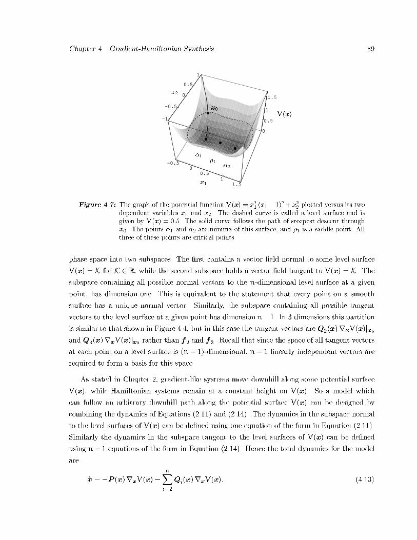
Chapter �� Gradient�Hamiltonian Synthesis ��
-0.50
0.51
1.5
-1
-0.5
0
0.5
1
0
0.5
1
1.5
-0.50
0.51
1 5
1
-0.5
0
0.5
1
0
0.5
1
1
V�x�x�
�
x�
x�
���
Figure ��� The graph of the potential function V�x� x�� �x� � �� � x�� plotted versus its twodependent variables x� and x�� The dashed curve is called a level surface and isgiven by V�x� ���� The solid curve follows the path of steepest descent throughx�� The points � and � are minima of this surface� and �� is a saddle point� Allthree of these points are critical points�
phase space into two subspaces� The �rst contains a vector �eld normal to some level surface
V�x� � K for K � R� while the second subspace holds a vector �eld tangent to V�x� � K� Thesubspace containing all possible normal vectors to the n�dimensional level surface at a given
point� has dimension one� This is equivalent to the statement that every point on a smooth
surface has a unique normal vector� Similarly� the subspace containing all possible tangent
vectors to the level surface at a given point has dimension n��� In � dimensions this partition
is similar to that shown in Figure ���� but in this case the tangent vectors are Q��x�rxV�x�jx�and Q��x�rxV�x�jx� rather than f� and f�� Recall that since the space of all tangent vectors
at each point on a level surface is �n � ���dimensional� n � � linearly independent vectors are
required to form a basis for this space�
As stated in Chapter �� gradient�like systems move downhill along some potential surface
V�x�� while Hamiltonian systems remain at a constant height on V�x�� So a model which
can follow an arbitrary downhill path along the potential surface V�x� can be designed by
combining the dynamics of Equations ������ and ������� The dynamics in the subspace normal
to the level surfaces of V�x� can be de�ned using one equation of the form in Equation �������
Similarly the dynamics in the subspace tangent to the level surfaces of V�x� can be de�ned
using n� � equations of the form in Equation ������� Hence the total dynamics for the model
are
�x � �P �x�rxV�x� �
nXi��
Qi�x�rxV�x�� ������
Chapter �� Gradient�Hamiltonian Synthesis ��
For this model the number and location of equilibria is determined by the function V�x�� while
the manner in which the equilibria are approached is determined by the matrices P �x� and
Qi�x�� The critical points of V�x� are the only equilibria of this system� If the graph of
the potential function V�x� is �� bounded below �i�e� V�x� � Bl � x � Rn � where Bl is
a constant�� �� radially unbounded �i�e� limkxk��V�x� � �� � and �� has only a �nite
number of isolated critical points �i�e� in some neighborhood of every point where rxV�x� �
there are no other points where the gradient vanishes�� then the system in Equation ������
satis�es the conditions of Theorem ���� Therefore the system will converge to one of the
critical points of V�x� for all initial conditions� Note that this system is capable of all downhill
trajectories along the potential surface only if the n� � vectors Qi�x�rxV�x� � i � �� � � � �n
are linearly independent at every point x� This means that the rank of the n �n� �� matrix
�Q�rV Q�rV � � � QnrV� is n � � for all x� If the number of states n is even� then it is
always possible to construct a system of n � � linearly independent vectors which vanish at
rxV�x� � � This is due to the following reason� If V�x� satis�es the � criteria given above�
then there is some closed and bounded region which contains all of the critical points� Outside
this region� the level surfaces of V�x� can be smoothly transformed into the sphere Sn�� �i�e�
for su�ciently large K� there is a homeomorphism from V�x� � K to Sn���� According to
Milnor ������� a result due to Brouwer states that Sn�� has a smooth �eld of non�zero tangent
vectors if and only if n� � is odd� which implies that n is even�
In the remainder of this section a learning rule for systems similar to those in Equation ������
is introduced� The only change made to the system is the addition of a term for the system
inputs� In Equation ������ the number and location of equilibria can be controlled using
the potential function V�x�� while the manner in which the equilibria are approached can be
controlled with the matrices P �x� andQi�x�� If it is assumed that the locations of the equilibria
are known� then a potential function which has these critical points can be constructed using
Equation ������ The problem of system identi�cation is thereby reduced to the problem of
parametrizing the matrices P �x� and Qi�x� and �nding the parameter values which cause this
model to best emulate the actual system� If the elements P �x� and Qi�x� are correctly chosen�
then a learning rule can be designed which makes the model dynamics converge to that of the
actual system�
Speci�cally� choose each element of these matrices to have the form
Prs �nXj��
l��Xk��
�rsjk �k�xj� and Qrs �nX
j��
l��Xk��
�rsjk �k�xj�� ������
where f���xj�� ���xj�� � � � � �l���xj�g and f���xj�� ���xj�� � � � � �l���xj�g are a set of l orthogonal
polynomials which depend on the state xj � There is a set of such polynomials for every state xj �
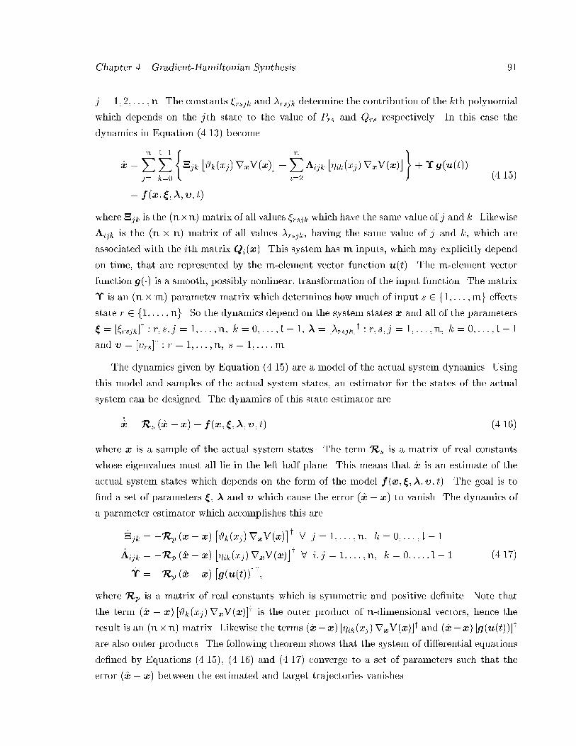
Chapter �� Gradient�Hamiltonian Synthesis ��
j � �� �� � � � �n� The constants �rsjk and �rsjk determine the contribution of the kth polynomial
which depends on the jth state to the value of Prs and Qrs respectively� In this case the
dynamics in Equation ������ become
�x �
nXj��
l��Xk��
��jk
��k�xj�rxV�x�
��
nXi��
�ijk
��ik�xj�rxV�x�
����g�u�t��
� f�x� ������ t�
������
where�jk is the �n n� matrix of all values �rsjk which have the same value of j and k� Likewise
�ijk is the �n n� matrix of all values �rsjk� having the same value of j and k� which are
associated with the ith matrix Qi�x�� This system has m inputs� which may explicitly depend
on time� that are represented by the m�element vector function u�t�� The m�element vector
function g��� is a smooth� possibly nonlinear� transformation of the input function� The matrix
� is an �n m� parameter matrix which determines how much of input s � f�� � � � �mg e�ects
state r � f�� � � � �ng� So the dynamics depend on the system states x and all of the parameters
� � ��rsjk�y � r� s� j � �� � � � �n� k � �� � � � � l� �� � � ��rsjk�
y � r� s� j � �� � � � �n� k � �� � � � � l� �
and � � ��rs�y � r � �� � � � �n� s � �� � � � �m�
The dynamics given by Equation ������ are a model of the actual system dynamics� Using
this model and samples of the actual system states� an estimator for the states of the actual
system can be designed� The dynamics of this state estimator are
� x �Rs � x� x� � f�x� ������ t� ������
where x is a sample of the actual system states� The term Rs is a matrix of real constants
whose eigenvalues must all lie in the left half plane� This means that x is an estimate of the
actual system states which depends on the form of the model f�x� ������ t�� The goal is to
�nd a set of parameters �� � and � which cause the error � x� x� to vanish� The dynamics of
a parameter estimator which accomplishes this are
��jk � �Rp � x� x���k�xj�rxV�x�
�y � j � �� � � � �n� k � �� � � � � l� �
��ijk � �Rp � x� x���ik�xj�rxV�x�
�y � i� j � �� � � � �n� k � �� � � � � l� �
�� � �Rp � x� x��g�u�t��
�y�
������
where Rp is a matrix of real constants which is symmetric and positive de�nite� Note that
the term � x � x� ��k�xj�rxV�x��y is the outer product of n�dimensional vectors� hence the
result is an �n n� matrix� Likewise the terms � x�x� ��ik�xj�rxV�x��y and � x�x� �g�u�t���yare also outer products� The following theorem shows that the system of di�erential equations
de�ned by Equations ������� ������ and ������ converge to a set of parameters such that the
error � x� x� between the estimated and target trajectories vanishes�
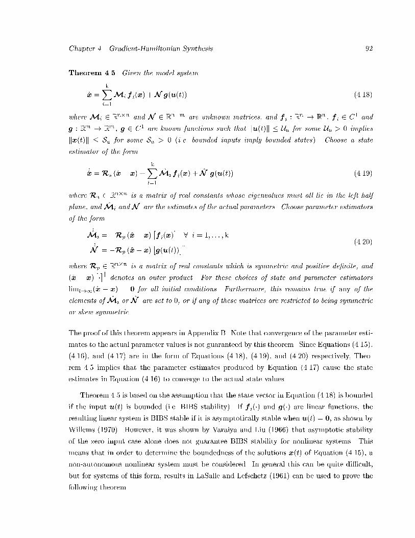
Chapter �� Gradient�Hamiltonian Synthesis ��
Theorem ���� Given the model system
�x �kXi��
Mi f i�x� �N g�u�t�� ������
where Mi � Rn�n and N � R
n�m are unknown matrices� and f i � Rn � R
n � f i � C� and
g � Rm � Rm � g � C� are known functions such that ku�t�k � Uu for some Uu � � implies
kx�t�k � Su for some Su � � �i�e� bounded inputs imply bounded states�� Choose a state
estimator of the form
� x �Rs � x� x� �kX
i��
Mi f i�x� � N g�u�t�� ������
where Rs � Rn�n is a matrix of real constants whose eigenvalues must all lie in the left half
plane� and Mi and N are the estimates of the actual parameters� Choose parameter estimators
of the form
� Mi � �Rp � x� x��f i�x�
�y � i � �� � � � �k
� N � �Rp � x� x��g�u�t��
�y ������
where Rp � Rn�n is a matrix of real constants which is symmetric and positive de�nite� and
� x � x����y denotes an outer product� For these choices of state and parameter estimators
limt��� x � x� � for all initial conditions� Furthermore� this remains true if any of the
elements of Mi or N are set to �� or if any of these matrices are restricted to being symmetric
or skew�symmetric�
The proof of this theorem appears in Appendix B� Note that convergence of the parameter esti�
mates to the actual parameter values is not guaranteed by this theorem� Since Equations �������
������� and ������ are in the form of Equations ������� ������� and ������ respectively� Theo�
rem ��� implies that the parameter estimates produced by Equation ������ cause the state
estimates in Equation ������ to converge to the actual state values�
Theorem ��� is based on the assumption that the state vector in Equation ������ is bounded
if the input u�t� is bounded �i�e� BIBS stability�� If f i��� and g��� are linear functions� the
resulting linear system is BIBS stable if it is asymptotically stable when u�t� � � as shown by
Willems ������� However� it was shown by Varaiya and Liu ������ that asymptotic stability
of the zero input case alone does not guarantee BIBS stability for nonlinear systems� This
means that in order to determine the boundedness of the solutions x�t� of Equation ������� a
non�autonomous nonlinear system must be considered� In general this can be quite di�cult�
but for systems of this form� results in LaSalle and Lefschetz ������ can be used to prove the
following theorem�
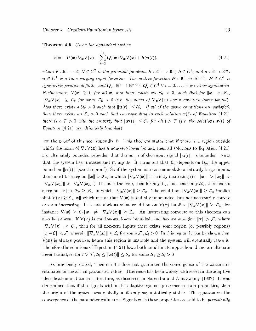
Chapter �� Gradient�Hamiltonian Synthesis ��
Theorem ���� Given the dynamical system
�x � �P �x�rxV�x� �
nXi��
Qi�x�rxV�x� � h�u�t��� ������
where V � Rn � R� V � C� is the potential function� h � Rm � Rn � h � C�� and u � R � R
m �
u � C� is a time varying input function� The matrix function P � Rn � Rn�n � P � C� is
symmetric positive de�nite� and Qi � Rn � R
n�n � Qi � C� � i � �� � � � �n are skew�symmetric�
Furthermore� V�x� � � for all x� and there exists an Fu � �� such that for kxk � Fu�
krxV�x�k � Lu for some Lu � � �i�e� the norm of rxV�x� has a non�zero lower bound��
Also there exists a Uu � � such that ku�t�k � Uu� If all of the above conditions are satis�ed�
then there exists an Su � � such that corresponding to each solution x�t� of Equation ������
there is a T � � with the property that kx�t�k � Su for all t � T �i�e� the solutions x�t� of
Equation ������ are ultimately bounded��
For the proof of this see Appendix B� This theorem states that if there is a region outside
which the norm of rxV�x� has a non�zero lower bound� then all solutions to Equation ������
are ultimately bounded provided that the norm of the input signal ku�t�k is bounded� Note
that the system has n states and m inputs� It turns out that Lu depends on Uu� the upper
bound on ku�t�k �see the proof�� So if the system is to accommodate arbitrarily large inputs�
there must be a region kxk � Fm in which krxV�x�k is strictly increasing �i�e� kx�k � kx�k �krxV�x��k � krxV�x��k�� If this is the case� then for any Lu� and hence any Uu� there exists
a region kxk � Fu � Fm in which krxV�x�k � Lu� The condition krxV�x�k � Lu implies
that V�x� � Lukxk which means that V�x� is radially unbounded� but not necessarily convex
or even increasing� It is not obvious what condition on V�x� implies krxV�x�k � Lu� for
instance V�x� � Lukxk �� krxV�x�k � Lu� An interesting converse to this theorem can
also be proven� If V�x� is continuous� lower bounded� and has some region kxk � Fu where
krxV�x�k � Lu� then for all non�zero inputs there exists some region �or possibly regions�
kx�Ck � Fl wherein krxV�x�k � Ll for some Fl�Ll � �� In this region it can be shown that
�V�x� is always positive� hence this region is unstable and the system will eventually leave it�
Therefore the solutions of Equation ������ have both an ultimate upper bound and an ultimate
lower bound� so for t � T � Sl � kx�t�k � Su for some Su � Sl � ��
As previously stated� Theorem ��� does not guarantee the convergence of the parameter
estimates to the actual parameter values� This issue has been widely addressed in the adaptive
identi�cation and control literature� as discussed in Narendra and Annaswamy ������� It was
determined that if the signals within the adaptive system possessed certain properties� then
the origin of the system was globally uniformly asymptotically stable� This guarantees the
convergence of the parameter estimates� Signals with these properties are said to be persistently
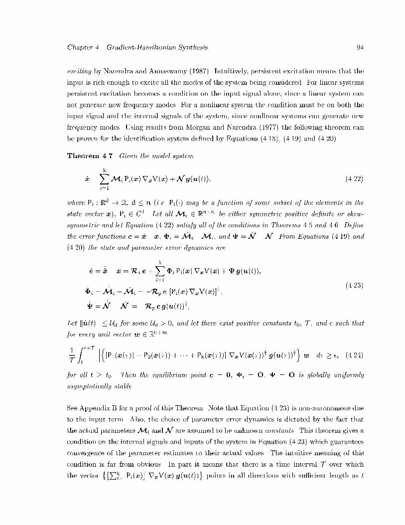
Chapter �� Gradient�Hamiltonian Synthesis ��
exciting by Narendra and Annaswamy ������� Intuitively� persistent excitation means that the
input is rich enough to excite all the modes of the system being considered� For linear systems
persistent excitation becomes a condition on the input signal alone� since a linear system can
not generate new frequency modes� For a nonlinear system the condition must be on both the
input signal and the internal signals of the system� since nonlinear systems can generate new
frequency modes� Using results from Morgan and Narendra ������ the following theorem can
be proven for the identi�cation system de�ned by Equations ������� ������ and �������
Theorem ���� Given the model system
�x �kXi��
Mi Pi�x�rxV�x� �N g�u�t��� ������
where Pi � Rd � R� d � n �i�e� Pi��� may be a function of some subset of the elements in the
state vector x�� Pi � C�� Let all Mi � Rn�n be either symmetric positive de�nite or skew�
symmetric and let Equation ������ satisfy all of the conditions in Theorems ��� and ���� De�ne
the error functions e � x�x� �i � Mi�Mi� and � � N �N � From Equations ������ and
������ the state and parameter error dynamics are
�e � � x� �x �Rs e�kXi��
�i Pi�x�rxV�x� �� g�u�t���
��i �� Mi � �Mi � �Rp e �Pi�x�rxV�x��y �
�� �� N � �N � �Rp e g�u�t��
y�
������
Let k �u�t�k � Ud for some Ud � �� and let there exist positive constants t�� T � and such that
for every unit vector w � Rn�m
�
TZ t�T
t
���n�P��x���� � P��x���� � � � � � Pk�x����� rxV�x����y g�u����yow��� d� � � ������
for all t � t�� Then the equilibrium point e � � �i � O� � � O is globally uniformly
asymptotically stable�
See Appendix B for a proof of this Theorem� Note that Equation ������ is non�autonomous due
to the input term� Also� the choice of parameter error dynamics is dictated by the fact that
the actual parametersMi and N are assumed to be unknown constants� This theorem gives a
condition on the internal signals and inputs of the system in Equation ������ which guarantees
convergence of the parameter estimates to their actual values� The intuitive meaning of this
condition is far from obvious� In part it means that there is a time interval T over which
the vector��P
ki��Pi�x�
� rxV�x� g�u�t���
points in all directions with su�cient length as t
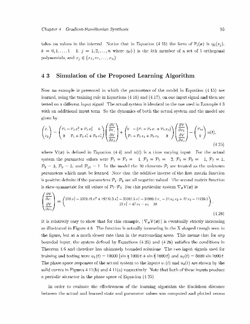
Chapter �� Gradient�Hamiltonian Synthesis ��
takes on values in the interval� Notice that in Equation ������ the form of Pi�x� is �k�xj��
k � �� �� � � � � l � �� j � �� �� � � � �n where �k��� is the kth member of a set of l orthogonal
polynomials� and xj � fx�� x�� � � � � xng�
��� Simulation of the Proposed Learning Algorithm
Now an example is presented in which the parameters of the model in Equation ������ are
learned� using the training rule in Equations ������ and ������� on one input signal and then are
tested on a di�erent input signal� The actual system is identical to the one used in Example ���
with an additional input term� So the dynamics of both the actual system and the model are
given by��x�
�x�
��
�P� � P� x
�� � P� x
�� �
� P� �P� x�� �P� x
��
�B��V
�x�
�V
�x�
�CA�
�� �fP � P x� � P� x�g
P �P x� � P� x� �
�B��V
�x�
�V
�x�
�CA�
�P��
�
�u�t��
������
where V�x� is de�ned in Equation ����� and u�t� is a time varying input� For the actual
system the parameter values were P� � P� � ��� P� � P� � ��� P� � P� � ��� P� � ��
P� � �� P� � �� and P�� � �� In the model the �� elements Pi are treated as the unknown
parameters which must be learned� Note that the additive inverse of the �rst matrix function
is positive de�nite if the parameters P� P� are all negative valued� The second matrix function
is skew�symmetric for all values of P� P�� For this particular system rxV�x� isB�
�V
�x�
�V
�x�
�CA �
���� x
�� � ������ x
�� � ����� x
�� � ������� x
�� � ������ x� � �x� x� � � x� � �����
��x�� � � x� � x� � ��
��
������
It is relatively easy to show that for this example� krxV�x�k is eventually strictly increasing
as illustrated in Figure ���� The function is actually increasing in the X�shaped trough seen in
the �gure� but at a much slower rate than in the surrounding areas� This means that for any
bounded input� the system de�ned by Equations ������ and ������ satis�es the conditions in
Theorem ��� and therefore has ultimately bounded solutions� The two input signals used for
training and testing were u��t� � ������sin �
� ���� t � sin �� ���� t
�and u��t� � ���� sin ���� t�
The phase space responses of the actual system to the inputs u��t� and u��t� are shown by the
solid curves in Figures �����b� and �����a� respectively� Note that both of these inputs produce
a periodic attractor in the phase space of Equation �������
In order to evaluate the e�ectiveness of the learning algorithm the Euclidean distance
between the actual and learned state and parameter values was computed and plotted versus
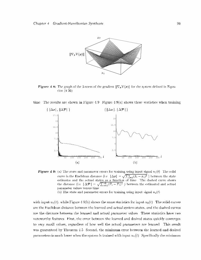
Chapter �� Gradient�Hamiltonian Synthesis ��
x�
x�
krxV�x�k
x�
x�
krxV�x�k
Figure ��� The graph of the ��norm of the gradient krxV�x�k for the system de�ned in Equa�tion �������
time� The results are shown in Figure ���� Figure ����a� shows these statistics when training
50 100 150 200 250 300
2.5
5
7.5
10
12.5
15
17.5
t
f k�xk� k�Pk g
�a�
50 100 150 200 250 300
2.5
5
7.5
10
12.5
15
t
f k�xk� k�Pk g
�b�
Figure ���� �a� The state and parameter errors for training using input signal u��t�� The solid
curve is the Euclidean distance �i�e� k�xk pP
�i����xi � xi�� � between the state
estimates and the actual states as a function of time� The dashed curve showsthe distance �i�e� k�Pk
pP��i��� �Pi �Pi�� � between the estimated and actual
parameter values versus time��b� The state and parameter errors for training using input signal u��t��
with input u��t�� while Figure ����b� shows the same statistics for input u��t�� The solid curves
are the Euclidean distance between the learned and actual system states� and the dashed curves
are the distance between the learned and actual parameter values� These statistics have two
noteworthy features� First� the error between the learned and desired states quickly converges
to very small values� regardless of how well the actual parameters are learned� This result
was guaranteed by Theorem ���� Second� the minimum error between the learned and desired
parameters is much lower when the system is trained with input u��t�� Speci�cally the minimum
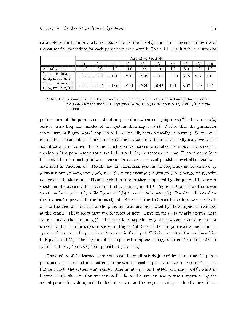
Chapter �� Gradient�Hamiltonian Synthesis ��
parameter error for input u��t� is ����� while for input u��t� it is ����� The speci�c results of
the estimation procedure for each parameter are shown in Table ���� Intuitively� the superior
Parameter VariableP� P� P� P� P� P P� P P� P��
Actual value ���� ���� � �� ���� ���� � �� �� ��� ��� ��Value estimatedusing input u��t�
����� ����� � ��� ����� ����� � �� ��� � �� � ���� � �
Value estimatedusing input u��t�
����� ����� � ��� ���� ����� ����� �� ���� ���� ���
Table ���� A comparison of the actual parameter values and the �nal values of the parameterestimates for the model in Equation ������ using both input u��t� and u��t� for theestimation�
performance of the parameter estimation procedure when using input u��t� is because u��t�
excites more frequency modes of the system than input u��t�� Notice that the parameter
error curve in Figure ����a� appears to be eventually monotonically decreasing� So it seems
reasonable to conclude that for input u��t� the parameter estimates eventually converge to the
actual parameter values� The same conclusion also seems to justi�ed for input u��t� since the
envelope of the parameter error curve in Figure ����b� decreases with time� These observations
illustrate the relationship between parameter convergence and persistent excitation that was
addressed in Theorem ���� Recall that in a nonlinear system the frequency modes excited by
a given input do not depend solely on the input because the system can generate frequencies
not present in the input� These conclusions are further supported by the plots of the power
spectrum of state x��t� for each input� shown in Figure ����� Figure �����a� shows the power
spectrum for input u��t�� while Figure �����b� shows it for input u��t�� The dashed lines show
the frequencies present in the input signal� Note that the DC peak in both power spectra is
due to the fact that neither of the periodic structures generated by these inputs is centered
at the origin� These plots have two features of note� First� input u��t� clearly excites more
system modes than input u��t�� This partially explains why the parameter convergence for
u��t� is better than for u��t�� as shown in Figure ���� Second� both inputs excite modes in the
system which are at frequencies not present in the input� This is a result of the nonlinearities
in Equation ������� The large number of spectral components suggests that for this particular
system both u��t� and u��t� are persistently exciting�
The quality of the learned parameters can be qualitatively judged by comparing the phase
plots using the learned and actual parameters for each input� as shown in Figure ����� In
Figure �����a� the system was trained using input u��t� and tested with input u��t�� while in
Figure �����b� the situation was reversed� The solid curves are the system response using the
actual parameter values� and the dashed curves are the response using the �nal values of the
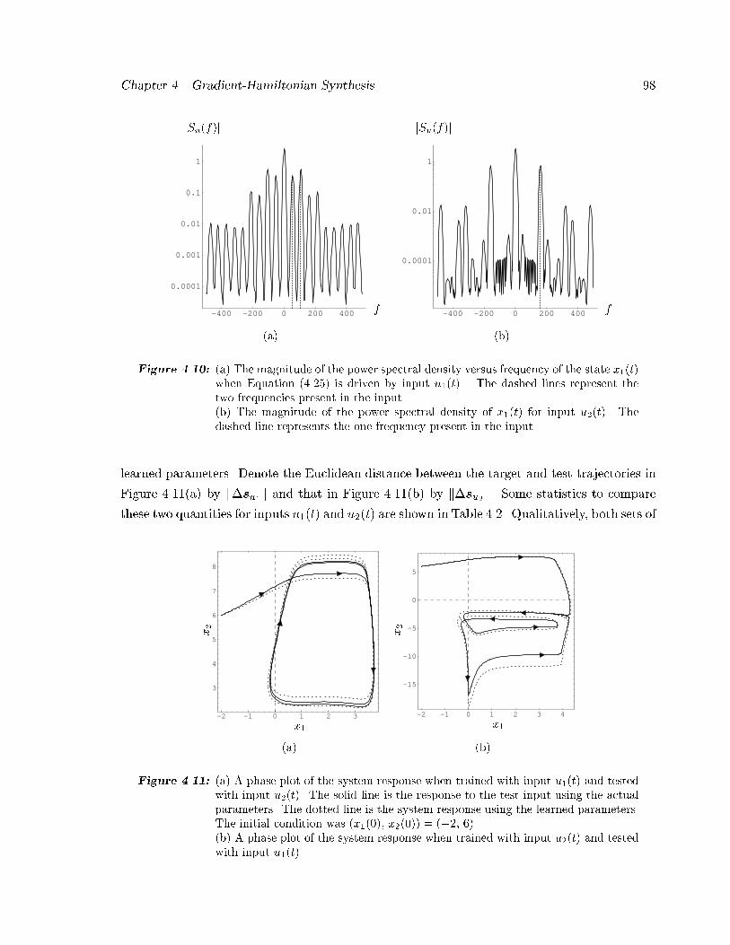
Chapter �� Gradient�Hamiltonian Synthesis ��
-400 -200 0 200 400
0.0001
0.001
0.01
0.1
1
f
jSu�f�j
�a�
-400 -200 0 200 400
0.0001
0.01
1
f
jSu�f�j
�b�
Figure ����� �a� The magnitude of the power spectral density versus frequency of the state x��t�when Equation ������ is driven by input u��t� � The dashed lines represent thetwo frequencies present in the input��b� The magnitude of the power spectral density of x��t� for input u��t�� Thedashed line represents the one frequency present in the input�
learned parameters� Denote the Euclidean distance between the target and test trajectories in
Figure �����a� by k$su�k and that in Figure �����b� by k$su�k� Some statistics to compare
these two quantities for inputs u��t� and u��t� are shown in Table ���� Qualitatively� both sets of
-2 -1 0 1 2 3
3
4
5
6
7
8
x�
x�
�a�
-2 -1 0 1 2 3 4
-15
-10
-5
0
5
x�
x�
�b�
Figure ����� �a� A phase plot of the system response when trained with input u��t� and testedwith input u��t�� The solid line is the response to the test input using the actualparameters� The dotted line is the system response using the learned parameters�The initial condition was �x����� x����� ���� ����b� A phase plot of the system response when trained with input u��t� and testedwith input u��t��
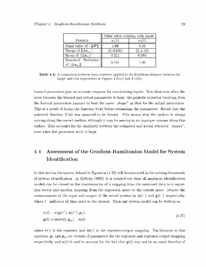
Chapter �� Gradient�Hamiltonian Synthesis ��
Value after training with inputStatistic u��t� u��t�
Final value of k$Pk ���� ����
Range of k$suik ��� ������ ��� �����
Mean of k$suik ����� �����
Standard Deviationof k$suik
����� ����
Table ���� A comparison between some statistics applied to the Euclidean distance between thetarget and test trajectories in Figures �� �a� and �� �b��
learned parameters give an accurate response for non�training inputs� Note that even when the
error between the learned and actual parameters is large� the periodic attractor resulting from
the learned parameters appears to have the same �shape as that for the actual parameters�
This is a result of �xing the function V�x� before estimating the parameters� Recall that the
potential function V�x� was assumed to be known� This means that the system is always
moving along the correct surface� although it may be moving in an improper manner along this
surface� This accounts for the similarity between the estimated and actual attractor �shapes�
even when the parameter error is large�
��� Assessment of the Gradient�Hamiltonian Model for System
Identi cation
In this section the system de�ned in Equation ������ will be examined in the existing framework
of system identi�cation� In Sj!oberg ������ it is pointed out that all nonlinear identi�cation
models can be viewed as the concatenation of a mapping from the measured data to a regres�
sion vector and another mapping from the regression space to the output space� Denote the
measurements of the input and output of the actual system by u�t�� and y�t�� respectively�
where t� indicates all time prior to the present� Then any system model can be written as
r�t� � r� y�t��� u�t���pr��
y�t� �m�r�t��pm� � n�t��������
where r��� is the regressor and m��� is the regressor�output mapping� Furthermore in this
equation� pr and pm are vectors of parameters for the regressor and regressor�output mapping
respectively� and n�t� is used to account for the fact that y�t� may not be an exact function of
Chapter �� Gradient�Hamiltonian Synthesis ���
the past data� The system models discussed in Section ��� are all of the form
�x �kXi��
Mi Pi�x�rxV�x� �N g�u�t��� �����a�
y � h�x�� �����b�
In the language of Sj!oberg ������ the model in Equation ������ is a nonlinear state space model
where Equation �����a� de�nes a regressor from previous actual inputs u�t� and previous virtual
outputs x�t� to the present virtual output� and Equation �����b� de�nes a mapping from the
virtual output space �i�e� regressor space� x�t� to the actual output space y�t�� Note that
this model is recurrent because the regressor depends on past outputs of the model� Also
note that both the regressor and the regressor�output mapping are estimated from data in
this identi�cation model� This stands in contrast to many identi�cation models� wherein the
regressor is �xed initially and only the regressor�output mapping is estimated from the data�
In Sj!oberg ������ two arguments are made for using state space models rather than trying to
model the input�output characteristics directly� First� by including parameters in the regressor
it may be possible to achieve a lower dimensional regression vector� Since the output vector
is estimated from the regression vector� lowering its dimension makes estimating the mapping
between the regressor space and the output space easier� Second� Sj!oberg ������ states that
input�output models are often numerically ill�conditioned� Hence it may be possible to achieve
models with better conditioning by using state space representations�
The system de�ned in Equation ������ has some desirable properties as a model for system
identi�cation� First� the stability of the model is easily established by using the conditions in
Theorem ���� Second� if the function V�x� is known� then Theorem ��� de�nes a parameter
estimator which is guaranteed to converge to a set of parameters for which the error between
the output of the model and that of the actual system is zero� Third� the conditions under
which the input is persistently exciting are speci�ed in Theorem ���� This theorem de�nes the
notion of an input which is su�ciently rich to allow the system to be identi�ed� Fourth� if
the functions V��� and g��� in Equation ������ are not parametrized� then linear optimization
techniques can be employed to �nd the parameters in the matrices Mi and N � This can be
seen by considering the Lyapunov function de�ned in the proof of Theorem ���
W� x� Mi� N � � � x� x�y Rp � x� x� �
Tr
�kXi��
� Mi �Mi
y � Mi �Mi
�� N �N
y � N �N
��
������
as the criterion function� Notice that the second term of this criterion function can be considered
as a regularization term which tries to keep the parameters close to their actual values� Since
Chapter �� Gradient�Hamiltonian Synthesis ���
the matrix Rp is symmetric and positive de�nite� W��� is clearly a quadratic form� This
means that W��� has a single global minimum� There are numerous computationally e�cient
optimization algorithms that can be used to �nd this minimum�
An unresolved issue concerning the models in Equation ������ is that of global identi�ability�
in the sense de�ned by Gustavsson� Ljung� and S!oderstr!om ������� A system is globally
identi�able if any two sets of parameters for which the systems behavior is the same are equal
or related by an equivalence relation� So for a globally identi�able system� each behavior has
a unique set of parameters which produce that behavior� This concept is discussed in the
context of neural networks in �Zbikowski ������� One undesirable property of the models in
Equation ������ is that they probably can not approximate an arbitrary nonlinear system� as
de�ned in Equation ������ This is because only a linear interaction between the state vector
x and the input vector u is permitted by Equation ������� This means that at best these
systems can approximate any nonlinear systems whose state dynamics are �x � f�x� � g�u��
although there is no proof of this conjecture� Another undesirable property is that in order
to model general systems� the function V�x� must be parametrized� If parametrized versions
of the constructions in Cohen ������ are used� then the parametrization of the entire system
becomes nonlinear and one is forced to return to nonlinear optimization methods to estimate
the parameters�
In this chapter the the complementary characteristics of gradient and Hamiltonian systems
have been used to synthesize a class of nonlinear models for system identi�cation� A learning
algorithm was proposed� which under certain model restrictions� was proven to converge to a
set of parameters for which the error between the model output and that of the actual system
vanishes� In the next chapter some concluding remarks will be made� and some ideas for future
research put forward�
Chapter �
Conclusion
The work in this dissertation revolves around the development of a formalism which decomposes
system dynamics into the sum of dissipative �e�g� convergent� and conservative �e�g� periodic�
components� Intuitively� this can be viewed as decomposing the dynamics into a component
normal to some surface and components tangent to other surfaces� All of these surfaces may be
the same� but obviously this is not the general case� The method involves approximating the
actual system by a sum of products in which the terms in the product are the gradient of some
potential function and a matrix function� in other wordsPk
i��M i�x�rxFi�x�� The desired
outcome is for the transient behavior of the system to be modeled by the matrix functions
M i�x�� while the long term behavior is modeled by the potential functions Fi�x�� In this
dissertation� this decomposition was used for two purposes� First� it was applied to existing
neural network architectures to analyze their dynamic behavior� Although it was found that
this formulation incorporates many neural network models� the analysis of the resulting systems
was only partially successful�
The second application of this decomposition is to create models which learn to emulate the
behavior of actual systems� The premise of this approach is that the process of machine learning
can be considered in two stages� The �rst stage is the design of a parametrized model which is
capable of representing the qualitative behavior of the system to be learned� The second stage is
the construction of an algorithm to estimate the model parameters based on samples taken from
the actual system� This is exactly the approach employed in traditional system identi�cation
�e�g� Ljung and S!oderstr!om �������� as studied in the control theory literature� The research
in this dissertation has addressed both stages of this process� It is assumed that the behavior
of the systems to be modeled can be described by a set of �rst order ordinary di�erential
equations� The formulated model consists of a set of parametrized di�erential equations which
posses a speci�ed set of attractors� and whose parameters can be adjusted to �t speci�c data�
This means that the manner in which the attractors are approached is altered by changing
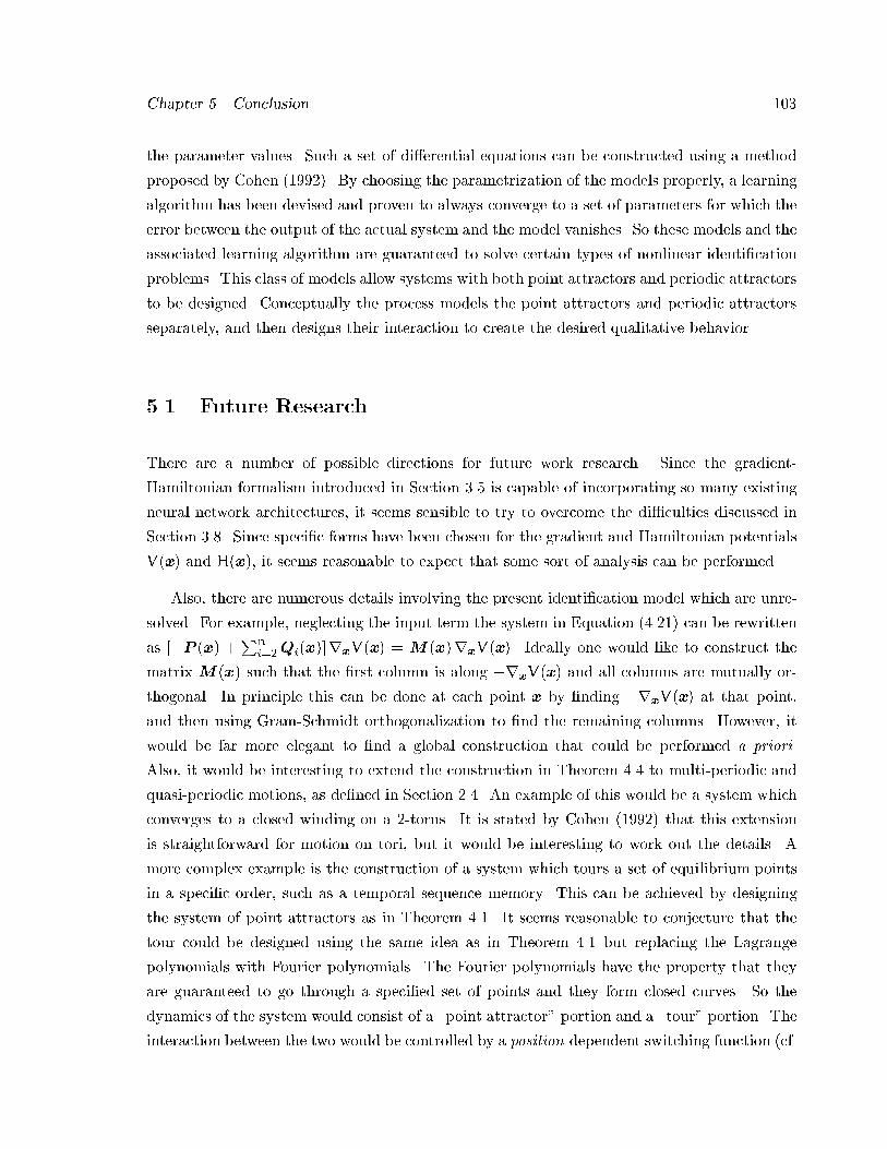
Chapter �� Conclusion ���
the parameter values� Such a set of di�erential equations can be constructed using a method
proposed by Cohen ������� By choosing the parametrization of the models properly� a learning
algorithm has been devised and proven to always converge to a set of parameters for which the
error between the output of the actual system and the model vanishes� So these models and the
associated learning algorithm are guaranteed to solve certain types of nonlinear identi�cation
problems� This class of models allow systems with both point attractors and periodic attractors
to be designed� Conceptually the process models the point attractors and periodic attractors
separately� and then designs their interaction to create the desired qualitative behavior�
��� Future Research
There are a number of possible directions for future work research� Since the gradient�
Hamiltonian formalism introduced in Section ��� is capable of incorporating so many existing
neural network architectures� it seems sensible to try to overcome the di�culties discussed in
Section ���� Since speci�c forms have been chosen for the gradient and Hamiltonian potentials
V�x� and H�x�� it seems reasonable to expect that some sort of analysis can be performed�
Also� there are numerous details involving the present identi�cation model which are unre�
solved� For example� neglecting the input term the system in Equation ������ can be rewritten
as ��P �x� �Pn
i��Qi�x��rxV�x� � M�x�rxV�x�� Ideally one would like to construct the
matrix M�x� such that the �rst column is along �rxV�x� and all columns are mutually or�
thogonal� In principle this can be done at each point x by �nding �rxV�x� at that point�
and then using Gram�Schmidt orthogonalization to �nd the remaining columns� However� it
would be far more elegant to �nd a global construction that could be performed a priori�
Also� it would be interesting to extend the construction in Theorem ��� to multi�periodic and
quasi�periodic motions� as de�ned in Section ���� An example of this would be a system which
converges to a closed winding on a ��torus� It is stated by Cohen ������ that this extension
is straightforward for motion on tori� but it would be interesting to work out the details� A
more complex example is the construction of a system which tours a set of equilibrium points
in a speci�c order� such as a temporal sequence memory� This can be achieved by designing
the system of point attractors as in Theorem ���� It seems reasonable to conjecture that the
tour could be designed using the same idea as in Theorem ��� but replacing the Lagrange
polynomials with Fourier polynomials� The Fourier polynomials have the property that they
are guaranteed to go through a speci�ed set of points and they form closed curves� So the
dynamics of the system would consist of a �point attractor portion and a �tour portion� The
interaction between the two would be controlled by a position dependent switching function �cf�
Chapter �� Conclusion ���
the function R��� in Theorem ���� which would switch between the �point attractor portion
and a �tour portion at certain locations in phase space�
Regarding the systems in Equation ������� there are three unresolved system identi�cation
issues� One is to speci�cally characterize the class of input functions which are persistently
exciting for the model de�ned in Equation ������� Recall that an input which is persistently
exciting leads to convergence of the parameters� as shown in Theorem ���� Speci�cally� this
involves �nding conditions on the input u�t� which guarantee that the condition de�ned in
Equation ������ is satis�ed� The second item is to determine whether the model in Equa�
tion ������ is globally identi�able� Roughly speaking this means that each system behavior has
a unique set of parameters which produce that behavior� This is� of course� never true with
respect to certain transformations� such as reordering the states� The third project would be to
determine conditions on Equation ������ which guarantee its controllability and observability�
A system is controllable if any initial state can be transferred to any �nal state in a �nite time
using the appropriate input� A system is observable if its present state values �i�e� the values
of the elements in x� can be computed from measurements of its outputs �i�e� the values of
the elements in y�� The generalization of these ideas from linear to nonlinear systems is dis�
cussed in Isidori ������� The fourth issue is one of implementation� Although� Theorem ����
gives a set of di�erential equations for �nding the parameters which cause the error between
the desired and model trajectories to vanish� solving these di�erential equations on a digital
computer is not necessarily a fast way to arrive at this solution� It would probably be faster
to use the function in Equation ������ as a criterion function and employ linear optimization
techniques to �nd its minimum�
A signi�cant unanswered question about the models in Equation ������ is their universal�
ity� A system which is universal can approximate any dynamical system� At the moment
this is certainly not the case because only the transient behavior represented by the matrix
functions P �x� and Qi�x� is being modeled� Clearly� in order to model the behavior of a
general system� the long term behavior represented by the potential function V�x� must also
be learned from data� As stated previously� �nding asymptotically stable structures in data is
usually straightforward� In that sense learning V�x� from data appears fairly trivial� However�
unstable structures can have a signi�cant impact on the system dynamics� and these are in
general very di�cult to locate� The investigation of constructive algorithms to synthesize the
potential function V�x� would be a fascinating project� Combined with the existing learning
algorithm for the transient behavior� this construction would constitute a design technique for
dynamical systems with arbitrary behavior which would have applications in control systems�
optimization� and analog circuit design� Also this type of construction might give insight on
how to decompose nonlinear dynamical systems on a behavioral basis� Decomposition on a
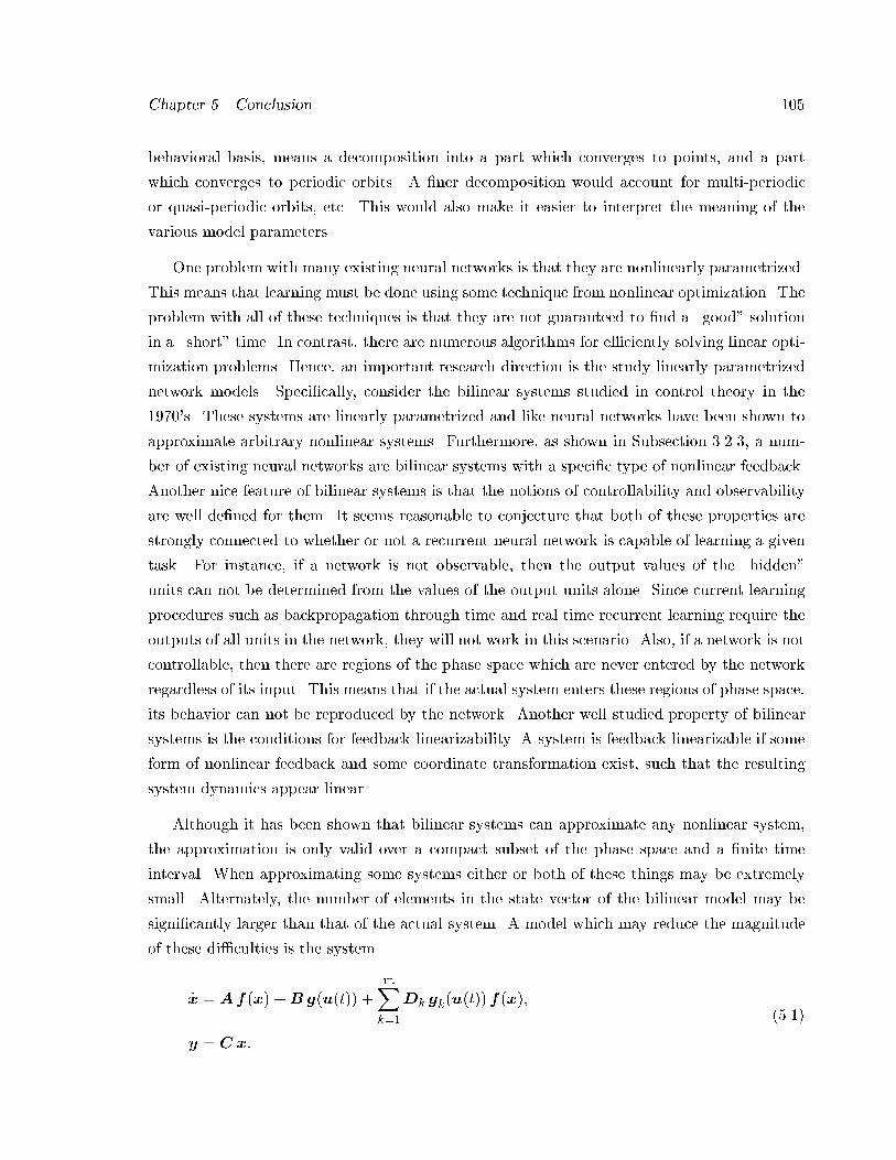
Chapter �� Conclusion ���
behavioral basis� means a decomposition into a part which converges to points� and a part
which converges to periodic orbits� A �ner decomposition would account for multi�periodic
or quasi�periodic orbits� etc� This would also make it easier to interpret the meaning of the
various model parameters�
One problem with many existing neural networks is that they are nonlinearly parametrized�
This means that learning must be done using some technique from nonlinear optimization� The
problem with all of these techniques is that they are not guaranteed to �nd a �good solution
in a �short time� In contrast� there are numerous algorithms for e�ciently solving linear opti�
mization problems� Hence� an important research direction is the study linearly parametrized
network models� Speci�cally� consider the bilinear systems studied in control theory in the
����s� These systems are linearly parametrized and like neural networks have been shown to
approximate arbitrary nonlinear systems� Furthermore� as shown in Subsection ������ a num�
ber of existing neural networks are bilinear systems with a speci�c type of nonlinear feedback�
Another nice feature of bilinear systems is that the notions of controllability and observability
are well de�ned for them� It seems reasonable to conjecture that both of these properties are
strongly connected to whether or not a recurrent neural network is capable of learning a given
task� For instance� if a network is not observable� then the output values of the �hidden
units can not be determined from the values of the output units alone� Since current learning
procedures such as backpropagation through time and real time recurrent learning require the
outputs of all units in the network� they will not work in this scenario� Also� if a network is not
controllable� then there are regions of the phase space which are never entered by the network
regardless of its input� This means that if the actual system enters these regions of phase space�
its behavior can not be reproduced by the network� Another well studied property of bilinear
systems is the conditions for feedback linearizability� A system is feedback linearizable if some
form of nonlinear feedback and some coordinate transformation exist� such that the resulting
system dynamics appear linear�
Although it has been shown that bilinear systems can approximate any nonlinear system�
the approximation is only valid over a compact subset of the phase space and a �nite time
interval� When approximating some systems either or both of these things may be extremely
small� Alternately� the number of elements in the state vector of the bilinear model may be
signi�cantly larger than that of the actual system� A model which may reduce the magnitude
of these di�culties is the system
�x � Af�x� �Bg�u�t�� �
mXk��
Dk gk�u�t��f�x��
y � C x�
�����
Chapter �� Conclusion ���
Since a bilinear system is universal� it seems likely that this system is also universal� probably
with some restrictions on the class of functions that can be used for f��� and g���� Since this isa rather general nonlinear system� properties such as stability probably can not be established
without making assumptions about the form of f��� and g���� One starting point would be
to assume that f��� and g��� are the gradient of two di�erent potential functions� and see if
something similar to Theorem ��� can be proved for these systems� These systems would also
be amenable to a two stage learning procedure in which stage one is a linear optimization of
the parameters� A� B� C� and Dk� and stage two is the construction of the functions f��� andg����
Appendix A
Basic Topology
First� the notion of a function is de�ned� Given two sets X and Y� a subset f � X�Y is a function if for
every x � X there exists an element y � Y such that �x�y� � f � and �x�y� � f and �x� �y� � f implies
that y �y� So a function is a mapping f from the set X to the set Y� denoted f � X Y� such that for
every x � X there exists a unique y � Y� The set X is called the domain and Y is called the range� The
notions of the image and the graph of a function are de�ned below�
De�nition A��� The image of the function f � X Y is the subset of Y consisting of all points such
that y f �x� for some point x � X�
De�nition A��� The graph of the function f � X Y is the subset of all ordered pairs �x�y�� where
x � X and y � Y� which contains all ordered pairs of the form �x�f �x���
So the image of the function f is that part of the set Y into which all members of X are mapped� The
graph is the set of points in the set X � Y de�ned by the function� This corresponds with the usual
intuition of a graph� For example� the image of the function f � R R � f�x� x� is the set �����
and the graph is the set of all ordered pairs �x� x���
Two of the fundamental concepts in topology are the ideas of the norm of a vector� and the inner
product of two vectors� Intuitively� the norm of vector is related to the length of that vector� while the
inner product of two vectors is related to the angle between the vectors� The following formal de�nitions
of these two ideas are taken from Hirsch and Smale � �����
De�nition A��� A norm is any function k � k � Rn R having the three properties of� �� positive
de�niteness� kxk � �� and kxk � if and only if x ���� satisfying Minkowski s inequality kx� yk �
kxk� kyk��� kKxk jKj kxk where j � j denotes the absolute value and K � R�
De�nition A��� An inner product is any function h� � �i � Rn �Rn R having the three properties of�
�� symmetry hx�yi hy�xi� �� bilinearity hx� y� zi hx� zi � hy� zi and hKx�yi K hx�yi� where
K � R� �� positive de�niteness hx�xi � �� and hx�xi � if and only if x ��
The relationship between these two concepts is de�ned by the Cauchy�Schwarz inequality� which is
hx�yi � kxk kyk� Note that the equality must hold when x y� Another function which has many of
Appendix A� Basic Topology ���
the properties of a norm� but which depends on two variables� is a metric�
De�nition A�� A metric is any function D � Rn �Rn R having the three properties of� �� positive
de�niteness� D�x�y� � �� and D�x�y� � if and only if x y� �� symmetry D�x�y� D�y�x�� ��
satisfying Minkowski s inequality D�x� z� � D�x�y� �D�y� z��
Conceptually a metric de�nes a way to measure the distance between two vectors� A metric is often
called a Riemannian metric when referring to the distance measure used in the phase space of a set of
di�erential equations� In this dissertation� the metric given two vectors x�y � Rn is de�ned to be the
norm of the di�erence between the vectors DE�x�y� kx� yk� which is called the Euclidean metric�
Another important function� which is similar to the inner product� is the ��form�
De�nition A�� A ��form is any function F � Rn � Rn R having the two properties of� �� skew�
symmetry F�x�y� �F�y�x�� �� bilinearity F�x � y� z� F�x� z� � F�y� z� and F�Kx�y� K F�x�y��
where K � R�
Conceptually a ��form de�nes a way to measure the area of the parallelogram between two vectors� A
��form is often called a symplectic form when referring to the area measure used in the phase space of
a set of di�erential equations�
A very important class of topological spaces are those in which the concept of distance between two
elements is de�ned� This combination of a set and metric de�ned on that set is called a metric space�
The formal de�nition� as given in Christenson and Voxman � ����� follows�
De�nition A��� A metric space is a pair �S�D� where S is a set and D � S� S ���� is a metric�
The set Rn with the metric DE is called a Euclidean metric space and is denoted by En� Given a
function f � a metric D de�ned on the domain of f � and a possibly di�erent metric �D on the range� the
notion of continuity of f can be de�ned� Intuitively� a function f is continuous if the value of f�x�� is
close to that of f �x� when x� is close to x�
De�nition A��� The function f � X Y is continuous at the point x� � X if and only if for each � �
there exists a � � such that x � X and D�x��x� � � implies �D�f�x���f �x�� � �� The function f is
continuous if it is continuous at every point x � X�
For example� the function x� sin��x
is continuous at x �� but the function �
xsin��x�
is not� A
function f is said to be a member of the set Cr if f is continuous and can be di�erentiated r times with
each derivative also being a continuous function�
There are a number of notions which are important in studying metric spaces� One is the notion
of seperability� which intuitively means that every open set in the metric space can be constructed by
taking the union of elements from a countable basis set� A set is countable if it can be put into one�to�one
correspondence with some subset of the natural numbers N �i�e� � �� �� � � � �� For instance the set of all
rational numbers Q is countable�
Appendix A� Basic Topology ���
De�nition A� � A subset D of a space X is dense in X if and only if every non�empty open set in X
intersects D� A space X is separable if and only if X contains a countable dense subset�
For example� En is a separable metric space because the set of rational numbers Q is a countable dense
subset of R�
In topology� two spaces are considered equivalent if they can be deformed into one another by
stretching or bending without any tearing or glueing� A transformation which accomplishes this is
called a homeomorphism� More speci�cally� two spaces are homeomorphic if one can jump from one to
the other with no intermediate steps� This idea is formally de�ned in Christenson and Voxman � ����
as follows�
De�nition A���� A homeomorphism is a continuous function h � X Y whose inverse exists and is
also continuous�
For example� a sphere and a bowl are homeomorphic� likewise a torus and a cup are homeomorphic�
However� a sphere and a torus are not homeomorphic� Also� the interval �� � � and the line E� are
homeomorphic via the transformation h�x� x��jxj � Note that a homeomorphism is not required to
preserve lengths� angles� or any other geometrical notions�
Appendix B
Proofs for Chapter �
Proof of Theorem ��
The following lemma� which is proved in Narendra and Annaswamy � ����� is used in the proof of this
theorem�
Lemma B�� �Barbalat�� If �f�t� is bounded and�
limt��
R tt�jf� �j�d
� �
�
exists and is �nite� then
limt��
f �t� ��
Proof� De�ne the error quantities e� �i� and � as in Theorem ���� Subtract Equations ��� �� and ��� ��
to obtain the equation for �e� Since Mi and N are assumed to be constant� the equations for ��i� and�� are identical to those shown in Equation ��� ��� To show that the equilibrium point e �� �i O�
� O is globally stable� choose the Lyapunov function
W�e��i��� eyRp e� Tr
�kXi��
�yi �i ��y�
��
where Tr��� is the trace of the matrix in the argument� Since Rp is positive de�nite� W��� is positive
de�nite because the trace of a sum of matrix inner products is a quadratic form� Since both terms of
W��� are quadratic forms� W��� is radially unbounded� The time derivative of W��� is
�W �eyRp e� eyRp �e� Tr
�kXi��
��yi �i �
kXi��
�yi
��i � ��y� ��y ��
��
Using the fact that Tr�M � N � Tr�M � � Tr�N�� Tr�M yN� Tr�N yM �� and for M symmetric
wyM v vyMw� the time derivative can be rewritten as
�W ey�RpRs �R
ysRp
�e� �
kXi��
eyRp�i f i�x� � �eyRp� g�u�t�� � Tr
��
kXi��
��y
i �i � � ��y�
�� �B� �
Substituting in the adaptive laws gives
�W ey�RpRs �Ry
sRp
�e� �
kXi��
eyRp�i f i�x� � �eyRp� g�u�t��
� Tr
���
kXi��
f i�x� eyRp�i � � g�u�t�� eyRp�
��

Appendix B� Proofs for Chapter � ���
Using the fact that Tr�wvy� vyw� the time derivative can be reduced to
�W ey�RpRs �Ry
sRp
�e�
SinceRs has strictly negative eigenvalues� the solution to the equationRpRs �RysRp �Q� for any
symmetric positive de�nite matrix Q� is a symmetric positive de�nite matrix Rp�
� �W �eyQ� e � �
Therefore the equilibrium state of the error functions is globally uniformly stable� This implies that
e�t�� �i�t�� and ��t� are bounded for all t � t�� Since f i�x� and g�u�t�� are bounded for bounded
inputs� �e as de�ned in Equation ������� is bounded� Since Q� is positive de�nite and �W � ��
� �
Z �
t�
e� �yQ� e� � d ��
Therefore by Barbalat s Lemma limt��
e�t� ��
The following proof segments outline the technique used to prove that this result continues to be
true if the matrix � is restricted to being symmetric or skew�symmetric� It is apparent that these
arguments follow if any of the parameter matrices are restricted in this manner�
Case �� � is symmetric �i�e� �y ��
This can be insured by writing the adaptive law as
�� �
�
�Rp e g�u�t��y �
�Rp e g�u�t��y
y��
In this case Equation �B� � for �W becomes
�W � � �� �eyRp� g�u�t�� � Tr
��
��
�
nRp e g�u�t��y �
�Rp eg�u�t��y
yo�y�
�� � � � �
� � �� �eyRp� g�u�t�� � eyRp�y g�u�t�� � eyRp� g�u�t�� � � � �
�y�� ��
Case �� � is skew�symmetric �i�e� �y ���
This can be insured by writing the adaptive law as
�� �
�
�Rp e g�u�t��y �
�Rp e g�u�t��y
y��
In this case Equation �B� � for �W becomes
�W � � �� �eyRp� g�u�t�� � Tr
��
��
�
nRp e g�u�t��y �
�Rp eg�u�t��y
yo�y�
�� � � � �
� � �� �eyRp� g�u�t�� � eyRp�y g�u�t�� � eyRp� g�u�t�� � � � �
�y��� ��
The following proof segment outlines the technique used to prove that this result continues to be true
if any elements of the matrix � are set to �� Again� these arguments follow if any of the parameter
matrices are restricted in this manner�
Appendix B� Proofs for Chapter � ���
Case �� Any elements of � are set to �
This can be achieved by writing � as
�
gXi��
Ri�f Ci�
where g � n� and �f is the matrix containing all n� possible parameters� The leading matrix Ri
has a single in the diagonal position corresponding to the row of the desired element of �f � All
other elements of Ri are �� The trailing matrix Ci has a in the diagonal position corresponding
to the column of the desired element of �f � with all other elements being �� The appropriate
adaptive law in this case is
�� �
gXi��
Ri
�Rp e g�u�t��y
Ci�
In this case Equation �B� � for �W becomes
W � � � �� � eRp
�gXi��
Ri�f Ci
�g�u�t � Tr
��
�gXi��
Ri
�Rp eg�u�t
y Ci
�y � gXi��
Ri�f Ci
��A� � � � �
From the distributive property of matrix multiplication vyPg
i��M iw Pg
i�� vyM iw and�Pg
i��M i
y �Pgi��N i
Pg
i��
Pgj��M
yi N j � So the expression for �W becomes
W � � � �� �
gXi��
eRp
�Ri�f Ci
�g�u�t � Tr
��
gXi��
gXj��
hRi
�Rp e g�u�t
y Ci
iy �Rj �f Cj
��A� � � � �
�B���
If these two terms can be shown to cancel for a single value of i� then they will cancel for any
sum over di�erent i values� For a single i value the matrix Ri�f Ci contains only one non�zero
value� located in the uth row and the wth column� The result of the product Rp �Ri�f Ci� is
to select the uth column of Rp� The result of the product Rp �Ri�f Ci� g�u�t�� is to select the
wth row of g�u�t��� Hence the �rst term is
� eRp �Ri�f Ci� g�u�t�� �
nXk��
ek rku �uw gw� �B���
Similarly� for a single i value� the matrix Ri
�Rp eg�u�t��y
Ci contains only one non�zero value
located in the uth row and the wth column� Consideration of the form of Rp eg�u�t��y leads to
the conclusion that the single entry has the form
Ri
�Rp e g�u�t��y
Ci
nXk��
ek ruk gw�
The transpose of this matrix contains the above entry in the wth row and uth column� Likewise
the matrix Ri�f Ci contains a single non�zero value for each value of j� When j i this value
occurs in the uth row and the wth column and the result of the product�Ri
�Rp e g�u�t��y
Ci
�y�Ri�f Ci� is a matrix with a single non�zero entry in the uth position along the diagonal�
Appendix B� Proofs for Chapter � ���
When j i the single entry in Ri�f Ci occurs somewhere else and the result of the product�Ri
�Rp e g�u�t��y
Ci
�y�Ri�f Ci� is the zero matrix� So the second term is
Tr
��
gXi��
gXj��
hRi
�Rp eg�u�t
y Ci
iy �Rj �f Cj
��A � ��nX
k��
ek ruk �uw gwR
yp�Rp
� ��nX
k��
ek rku �uw gw�
�B���
Taking the sum of Equations �B��� and �B��� leads to the conclusion that the two terms in
Equation �B��� cancel for a single i value� Therefore they will also cancel for a sum over any set
of i values��
Proof of Theorem ��
The following lemma� which is proved in the reference� is used in the proof of this theorem�
Lemma B�� �LaSalle and Lefschetz �� ���� Let V�x� be a scalar function which for all x has
continuous �rst partial derivatives with the property that limkxk�� V�x� � If �V�x� � �� � � for
all x outside some closed and bounded set D� then the solutions of �x f �x� t� are ultimately bounded�
Proof� Since h��� is continuous� ku�t�k � Uu � kh�u�t��k � �Uu� It is given that krxV�x�k � Lu�
Choose Lu to be
krVk � Lu �Uu �
q�U�u � ��min �
��min
�
where � is a positive constant and �min is the smallest eigenvalue of P �x� in the region where kxk Fu�
Since P is symmetric positive de�nite� the smallest eigenvalue �min is real and positive�
� �min krVk�� krVk �Uu� � � �
It is given that khk � �Uu � �khk � � �Uu
� �min krVk�� krVk khk � � � �min krVk
�� krVk �Uu� � � �
By the Cauchy�Schwarz inequality krVk khk � jrVyhj
� �min krVk�� jrVyhj � � � �min krVk
�� krVk khk � ��
where j � j is the absolute value� For the absolute value jrVyhj � rVyh
� �min krVk��rVyh� � � �min krVk
�� jrVyhj � �
Since �min is the smallest eigenvalue of the matrix P �x�
� rVyP rV�rVyh� � � �minrVyrV�rVyh� � � �
� �rVyP rV�rVyh � ��
The quantity on the left side of the inequality is precisely �V�x� for Equation ���� �� Therefore krxV�x�k
� Lu � �V�x� � �� for all x such that kxk Fu�
Appendix B� Proofs for Chapter � ���
It is well known from real analysis thatRkrVk dx� k
RrV dxk�
�
ZkrVk dx�
����ZrV dx
���� ����ZLu dx
����� kV� ck kLu xk
By Minkowski s inequality kVk� kck � kV� ck�
� kVk� kck � kV� ck Lu kxk
Since V � � and since V and c are scalars
� V Lu kxk � jcj
Hence krxV�x�k � Lu � V�x� Lu kxk � limkxk�� V�x� � Note that the converse of this
implication is not true� Using these two results� it follows immediately from Lemma B�� that the
solutions x�t� of Equation ���� � are ultimately bounded� �
Proof of Theorem ���
Proof� Since Equation ������ satis�es all of the conditions of Theorem ���� its solutions kx�t�k are
bounded� Let f i�x� Pi�x�rxV�x� and note that k �f i�x�t��k k�fi�x
�xk � k�fi�xk k �xk� Since f i and g
are continuous� and kx�t�k and ku�t�k are bounded� kf i�x�t��k and kg�u�t��k are bounded� Therefore
k �xk kPk
i��Mi f i�x� �N g�u�t��k �Pk
i�� kMik kf i�x�k� kNk kg�u�t��k is bounded� Since f i is
continuously di�erentiable� �f i�x
is continuous� Since kx�t�k is bounded� k�fi�xk is bounded� Therefore
k �f i�x�t��k is bounded� since it is less than or equal to the product of bounded functions� Similarly
k �g�u�t��k k �g�u
�uk � k �g�uk k �uk� Since g is continuously di�erentiable� �g
�uis continuous� Since ku�t�k
is bounded� k �g�uk is bounded� Since it is given that k �u�t�k is bounded� k �g�u�t��k is bounded�
It is given that there exist positive constants t�� T � and � such that for every unit vector w � Rn�m
T
Z t�T
t
����P��x� �� � P��x� �� � � � �� Pk�x� ��� rxV�x� ��y g�u� ��y�w�� d � � � t � t��
�
T
Z t�T
t
���f��x� ��y f��x� ��y � � �fk�x� ��y g�u� ��y�wk�� d � � � t � t��
where wk � Rkn�m � With this inequality and the fact that k �f i�x�k and k �g�u�k are bounded� it follows
immediately from Theorem � in Morgan and Narendra � ���� that Equation ������ is globally uniformly
asymptotically stable� �
Bibliography
Ackley� D�� Hinton� G�� ! Sejnowski� T� � ����� A learning algorithm for Boltzmann machines� Cognitive
Science� � � �� ��" ���
Amari� S��I� � ����� Neural theory of association and concept"formation� Biological Cybernetics� �� ����
��" ���
Arnold� V� � ����� Mathematical methods of classical mechanics ��nd edition��� Vol� �� of Graduate
Texts in Mathematics� Springer�Verlag� Inc�� New York� NY�
Arnold� V� � ����� Ordinary di�erential equations ��rd edition�� Springer�Verlag� Inc�� Berlin� Germany�
Athans� M�� ! Falb� P� � ����� Optimal control An introduction to the theory and its applications�
Vol� � of Lincoln Laboratory Publications� McGraw�Hill� Inc�� New York� NY�
Bellman� R� � ����� Dynamic Programming� Princeton University Press� Princeton� NJ�
Carpenter� G� � ����� Neural network models for pattern recognition and associative memory� Neural
Networks� � ���� ���"����
Christenson� C�� ! Voxman� W� � ����� Aspects of topology� Vol� �� of Pure and Applied Mathematics�
Marcel Dekker� Inc�� New York� NY�
Cohen� M� � ����� The construction of arbitrary stable dynamics in nonlinear neural networks� Neural
Networks� � �� ��" ���
Cohen� M�� ! Grossberg� S� � ����� Absolute stability of global pattern formation and parallel memory
storage by competitive neural networks� IEEE Transactions on Systems� Man and Cybernetics�
�� ���� � �"����
Duarte� J�� ! Mendes� R� � ����� Deformation of Hamiltonian dynamics and constants of motion in
dissipative systems� Journal of Mathematical Physics� � ���� ���" ����
Elman� J� � ����� Finding structure in time� Cognitive Science� � ���� ��"� �
F#oldiak� P� � ����� Forming sparse representaions by local anti"Hebbian learning� Biological Cybernetics�
� ���� ��" ���
Franks� J� � ����� Homology and dynamical systems� Vol� �� of Regional Conference Series in Mathe�
matics� American Mathematical Society� Providence� RI�
Bibliography ���
Funahashi� K��I�� ! Nakamura� Y� � ����� Approximation of dynamical systems by continuous time
recurrent neural networks� Neural Networks� � ���� �� "����
Giles� C�� ! Maxwell� T� � ����� Learning� invariance� and generalization in high�order neural networks�
Applied Optics� �� ����� ����"�����
Giles� C�� Miller� C�� Chen� D�� Chen� H�� Sun� G�� ! Lee� Y� � ����� Learning and extracting �nite
state automata with second�order recurrent networks� Neural Computation� ���� ���"����
Grossberg� S� � ����� Contour enhancement� short term memory� and constancies in reverberating neural
networks� Studies in Applied Mathematics� � ���� � �"����
Grossberg� S� � ����� Pattern learning by functional"di�erential neural networks with arbitrary path
weights� In Grossberg� S� �Ed��� Studies of Mind and Brain Neural Principles of Learning� Per�
ception� Development� Cognition� and Motor Control� Vol� �� of Boston Studies in the Philosophy
of Science� pp� ��" ��� D� Reidel Publishing Co�� Dordrecht� Holland�
Grossberg� S� � ����� Nonlinear neural networks� Principles� mechanisms� and architectures� Neural
Networks� � � �� �"� �
Grossberg� S�� ! Somers� D� � �� �� Synchronized oscillations during cooperative feature linking in a
cortical model of visual perception� Neural Networks� ���� ���"����
Guckenheimer� J�� ! Holmes� P� � ����� Nonlinear oscillations� dynamical systems and bifurcations of
vector �elds� Vol� �� of Applied Mathematical Sciences� Springer�Verlag� Inc�� New York� NY�
Gustavsson� I�� Ljung� L�� ! S#oderstr#om� T� � ����� Identi�cation of processes in closed loop " Identi��
ability and accuracy aspects� Automatica� �� � �� ��"���
Hirsch� M� � ����� Convergent activation dynamics in continuous time networks� Neural Networks� � ����
�� "����
Hirsch� M�� ! Smale� S� � ����� Di�erential equations� dynamical systems� and linear algebra� Vol� ��
of Pure and Applied Mathematics� Academic Press� Inc�� San Diego� CA�
Hop�eld� J� � ����� Neural networks and physical systems with emergent collective computational
abilities� Proceedings of the National Academy of Sciences of the United States� �� ���� ����"�����
Horne� B�� ! Giles� C� � ����� An experimental comparison of recurrent neural networks� In Tesauro�
G�� Touretzky� D�� ! Leen� T� �Eds��� Advances in Neural Information Processing Systems Pro�
ceedings of the ��� Conference� pp� ���"���� The MIT Press�
Horne� B� � ����� Recurrent neural networks A functional approach� Ph�D� thesis� University of New
Mexico� Department of Electrical Engineering�
Isidori� A� � ����� Nonlinear control systems An introduction ��nd edition��� Vol� �� of Communications
and Control Engineering� Springer�Verlag� Inc�� Berlin� Germany�
Jordon� M�� ! Rumelhart� D� � ����� Forward models� Supervised learning with a distal teacher�
Cognitive Science� �� ���� ���"����
Bibliography ���
Kailath� T� � ����� Linear systems� Vol� � of Information and System Sciences� Prentice�Hall� Inc��
Englewood Cli�s� NJ�
Kan� A� R�� ! Timmer� G� � ����� Global optimization� In Nemhauser� G�� Kan� A� R�� ! Todd� M�
�Eds��� Optimization� Vol� of Handbooks in Operations Research and Management Science� pp�
�� "���� Elsevier Science Publishing Co�� New York� NY�
Khalil� H� � ����� Nonlinear systems� Macmillan Publishing Co�� New York� NY�
Kosko� B� � ����� Adaptive bidirectional associative memories� Applied Optics� �� ����� ����"�����
Kosko� B� � ����� Neural networks and fuzzy systems A dynamical systems approach to machine
intelligence� Prentice Hall� Inc�� Englewood Cli�s� NJ�
LaSalle� J� � ����� Asymptotic stability criteria� In Birkho�� G�� Bellman� R�� ! Lin� C� �Eds���
Hydrodynamic Instability� Vol� XIII of Proceedings of Symposia in Applied Mathematics� pp� ���"
���� American Mathematical Society�
LaSalle� J�� ! Lefschetz� S� � �� �� Stability by Lyapunov�s direct method� with applications � st edition���
Vol� � of Mathematics in Science and Engineering� Academic Press� Inc�� New York� NY�
Ljung� L�� ! S#oderstr#om� T� � ����� Theory and practice of recursive identi�cation� Vol� � of Signal
Processing� Optimization� and Control� The MIT Press� Cambridge� MA�
Luenberger� D� � ����� Linear and nonlinear programming ��nd edition�� Addison�Wesley Publishing
Co�� Inc�� Reading� MA�
Mendes� R�� ! Duarte� J� � �� �� Decomposition of vector �elds and mixed dynamics� Journal of
Mathematical Physics� �� ���� ���" ����
Mendes� R�� ! Duarte� J� � ����� Vector �elds and neural networks� Complex Systems� � � �� � "���
Milnor� J� � ����� Topology from a di�erentiable viewpoint� University Press of Virginia� Charlottesville�
VA�
Morgan� A�� ! Narendra� K� � ����� On the stability of non�autonomous di�erential equations �x
�A � B�t��x with skew�symmetric matrix B�t�� SIAM Journal of Control and Optimization�
� � �� ��" ���
Narendra� K�� ! Annaswamy� A� � ����� Persistent excitation in adaptive systems� International Journal
of Control� � �� ��" ���
Narendra� K�� ! Annaswamy� A� � ����� Stable adaptive systems� Prentice�Hall� Inc�� Englewood Cli�s�
NJ�
Narendra� K�� ! Parthasarathy� K� � ����� Identi�cation and control of dynamical systems using neural
networks� IEEE Transactions on Neural Networks� � � �� �"���
Newhouse� S� � ����� Nondensity of axiom A�a� on S�� In Chern� S��S�� ! Smale� S� �Eds��� Global
Analysis� Vol� XIV of Proceedings of Symposia in Pure Mathematics� pp� � "���� American
Mathematical Society�
Bibliography ���
Palis� J�� ! de Melo� W� � ����� Geometric theory of dynamical systems An introduction� Springer�
Verlag� Inc�� New York� NY�
Palis� J�� ! Smale� S� � ����� Structural stability theorems� In Chern� S��S�� ! Smale� S� �Eds��� Global
Analysis� Vol� XIV of Proceedings of Symposia in Pure Mathematics� pp� ���"�� � American
Mathematical Society�
Pearlmutter� B� � ����� Learning state space trajectories in recurrent neural networks� Neural Compu�
tation� � ���� ���"����
Pearlmutter� B� � ����� Dynamic Recurrent Neural Networks� Tech� rep� CMU"CS"��" ��� School of
Computer Science� Carnegie Mellon University� Pittsburg� PA�
Peixoto� M� � ����� Structural stablility on ��dimensional manifolds� Topology� � ���� � " ���
Psaltis� D�� Park� C�� ! Hong� J� � ����� Higher order associative memories and their optical implemen�
tations� Neural Networks� � ���� ��" ���
Ramacher� U� � ����� Hamiltonian dynamics of neural networks� Neural Networks� � ���� ���"����
Robinson� A�� ! Fallside� F� � ����� Static and dynamic error propagation networks with application to
speech coding� In Anderson� D� �Ed��� Advances in Neural Information Processing Systems� pp�
���"�� � American Institute of Physics�
Rumelhart� D�� Hinton� G�� ! Williams� R� � ����� Learning internal representations by error propaga�
tion� In Rumelhart� D�� McClelland� J�� ! The PDP Research Group �Eds��� Parallel distributed
processing Explorations in the microstructure of cognition� Volume � Foundations� pp� � �"����
The MIT Press� Cambridge� MA�
Saad� D� � ����� Training recurrent neural networks via trajectory modi�cation� Complex Systems�
� ���� � �"����
Salam� F�� Wang� Y�� ! Choi� M� � �� �� On the analysis of dynamic feedback neural nets� IEEE
Transactions on Circuits and Systems� �� ���� ��"�� �
Sato� M��A� � ����� A real time learning algorithm for recurrent analog neural networks� Biological
Cybernetics� �� ���� ���"�� �
Sj#oberg� J� � ����� Non�linear system identi�cation with neural networks� Ph�D� thesis� Link#oping
University� Department of Electrical Engineering�
Smale� S� � �� �� On gradient dynamical systems� Annals of Mathematics� � � �� ��"����
Smale� S� � ����� Structurally stable systems are not dense� American Journal of Mathematics� �� ����
�� "����
Sontag� E� � ����� Neural nets as system models and controllers� In Proceedings of the �th Yale Workshop
on Adaptive and Learning Systems� pp� ��"��� Yale University Press�
Spivak� M� � ����� A comprehensive introduction to di�erential geometry� Vol� � Publish or Perish�
Inc�� Berkeley� CA�
Bibliography ���
Varaiya� P�� ! Liu� R� � ����� Bounded�input bounded�output stability of nonlinear time�varying dif�
ferential systems� Journal of SIAM� Series A Control� ���� ���"����
Verhulst� F� � ����� Nonlinear di�erential equations and dynamical systems� Springer�Verlag� Inc��
Berlin� Germany�
Vidyasagar� M� � ����� Nonlinear systems analysis � st edition�� Prentice�Hall� Inc�� Englewood Cli�s�
NJ�
Willems� J� � ����� Stability theory of dynamical systems� John Wiley ! Sons� Inc�� New York� NY�
Williams� R�� ! Zipser� D� � ����� A learning algorithm for continually running fully recurrent neural
networks� Neural Computation� � ���� ���"����
Zak� M� � ����� Terminal attractors in neural networks� Neural Networks� � ���� ���"����
�Zbikowski� R� � ����� Recurrent neural networks Some control aspects� Ph�D� thesis� University of
Glasgow� Department of Mechanical Engineering�