The collection of magnetic gradiometer data using a con-figuration of two, three, or four magnetometers has becomecommonplace. One use of these data is to improve the accu-racy and resolution of the gridded total magnetic fieldbeyond what can be interpolated from a single magne-tometer. This is especially important for anomalies oversmall magnetic sources that lie between survey lines andover linear sources that strike obliquely to the survey lines.As an alternative to improved accuracy and resolution, onecan consider increasing the survey line spacing to obtain theequivalent total magnetic field, thereby reducing the sur-vey cost.

Gridding methods. The improved resolution and accuracyof the measured horizontal gradients, over the correspond-ing derivatives computed from total magnetic field, areclearly demonstrated in McMullan and McLellan (1997).Therefore, it is sensible to incorporate the measured gradi-ents when interpolating the total magnetic field. The lateralgradient (i.e., the horizontal gradient perpendicular to thesurvey line direction) is the most critical because it providesthe most information regarding the behavior of the mag-netic field in the gaps between the survey lines.

The gradient tensor method to compute the gradient-enhanced total magnetic field, incorporating the measuredtotal magnetic field and the two measured horizontal gra-dients (lateral or across-line, and longitudinal or along-line),is briefly described by Hogg (2004), and compared to othermethods with favorable results. The technical details of thetechnique are not given, so it is not possible to implementthe method for inclusion in this comparison.

This paper evaluates two conventional gridding tech-niques applied to aeromagnetic data, and two gradient-enhanced techniques. All are available as part of a widelyused commercial software package (OASIS montaj fromGeosoft). The conventional techniques are:

• Bidirectional gridding, which applies a spline (linear,Akima or cubic) along the survey lines and then acrossthe survey lines

• Minimum curvature gridding, which fits the data to aconstrained minimum curvature surface (Smith andWessel, 1990)

The first gradient enhancement technique is describedin Nelson (1994). The gridded total magnetic field is derivedin the Fourier domain from the leveled and gridded lateraland longitudinal gradients, using the generalized 3D Hilberttransform relations. It was implemented by Nelson as amethod of producing a leveled total magnetic field withoutthe need of conventional tie-line leveling. This assumes thatthe total field level errors are due to diurnal variation. Themeasured gradients are minimally affected by diurnal. Theproblem with this approach is that the longest wavelengthsin the total magnetic field generally produce small gradi-ents, with amplitudes below the noise levels of a typical sur-vey. Our approach is to level the gradients and use them tocompute a “pseudo” total magnetic field. We also grid theleveled total magnetic field and use it to apply a long wave-

length correction to the “pseudo” total magnetic field.The second gradient enhancement technique is described

in Hardwick (1999). It uses the measured lateral gradientfrom two wingtip-mounted sensors to extrapolate values ofthe total magnetic field onto “pseudolines” at a specifieddistance on either side of the survey line. These values arethen included in the interpolation of the total magnetic field.

To test the gridding techniques, standard data process-ing was applied. Extensive effort to prepare the best possi-ble product was not undertaken, as it would not simulatea production situation, and might hide some of the issuesassociated with each method.

Study area. A 105 848-line-km aeromagnetic survey wasflown over the Kapuskasing Structural Zone in northeast-ern Ontario using three different contractors (GSC, 2001).The geology of the survey area was described as follows:

The eastern extent of the survey area covers a portionof the Kapuskasing Structural Zone (KSZ) and covers alarge area west of this structure. The KSZ represents anoblique cross section exposing about 20 km of upper andmiddle Archean crust uplifted along an east-verging thrustfault in the central part of the Superior Province. In thesouth, it grades from greenschist facies supracrustal rocks

Gradient enhancement of the total magnetic fieldSTEPHEN REFORD, Paterson, Grant & Watson Limited, Toronto, Canada

JANUARY 2006 THE LEADING EDGE 59

Editor’s note: All grids utilized in the preparation of this paper may beobtained by contacting the author.

Figure 1. Total magnetic field image of the study area, prepared usingbidirectional gridding (subset area used in later figures outlined in black).

and granitic rocks of the Wawa Subprovince in the west togranulite facies gneisses representing the deepest part ofthe section, truncated against greenstone and granitic rocksof the Abitibi Subprovince in the east.

Further to the north, metasedimentary rocks of theQuetico Subprovince are uplifted and truncated againstgranitic rocks of the Opatica Subprovince. As the zone wasthe locus of major uplift of Archean crust and upper man-tle, it has excellent potential for mineral deposits withinrocks units that have tapped these deep seated sources suchas diamonds in kimberlites and lamprophyres, and phos-phates and rare earth metals in carbonates. In addition,there may be good potential for PGEs, base metals andindustrial minerals in mafic intrusions, anorthosite bodiessuch as the Shawmere complex and within greenstoneenclaves.

The surficial cover over most of the survey area is thin.Thicker accumulations of up to tens of meters of till andglaciolacustrine deposits occur in the northern portion ofthe survey area.

The survey lines were flown 200 m apart at 320° azimuth,and at a nominal terrain clearance of 100 m. The control lineswere flown 1600 m apart at 50° azimuth. The 10-Hz sam-pling results in magnetic values measured every 8 m or soalong the lines. One of the contractors, Goldak AirborneSurveys, employed a three-magnetometer configuration(two wingtip sensors mounted 14.8 m apart, and a tailstinger situated 9.8 m to the rear). The survey was con-tracted for a single sensor, so the magnetic data from thewingtip magnetometers were compensated and lag-cor-rected, but no further compilation was undertaken. Thedata from the tail magnetometer were subjected to standardleveling procedures.

Results of conventional gridding. All grids were preparedat a 25-m grid cell interval (i.e., one-eighth the line spacing).Some may consider this a small interval, but it provides abetter depiction of the spatial resolution with and withoutgradient enhancement, and also shows high-frequency noiseand aliasing associated with the gridding techniques.

Aliasing occurs due to the difference in sampling in the linedirection (8 m) compared to the sampling perpendicular tothe line direction (200 m). It may appear as “beading” alonglinear anomalies, stretching of anomalies in the wrong direc-tion or distorted anomaly shapes, particularly where theanomaly strike is at a low angle relative to the line direc-tion. Wherever smoothing has been applied, it consisted oftwo passes of a 3�3 space-domain Hanning filter. All shad-ing is from the northwest, in the flightline direction.

60 THE LEADING EDGE JANUARY 2006

Figure 2. Enhanced residual image computed from the total magneticfield for a portion of the study area, prepared using bidirectional gridding.

Figure 3. Enhanced residual image computed from the total magneticfield for a portion of the study area, prepared using bidirectional griddingand smoothed.

Figure 4. Enhanced residual image computed from the total magneticfield for a portion of the study area, prepared using minimum curvaturegridding.

The enhanced residual is used as a high-frequencyenhancement to examine the detail in the various grids. Itis computed by applying two passes of a Hanning 3�3smoothing filter to the total magnetic field grid, and thensubtracting the smoothed grid from the original. Qual-itatively, it is quite similar to a second vertical derivativeand is useful for examining short-wavelength anomaliesand high-frequency noise.

Figure 1 shows the total magnetic field interpolatedusing bidirectional gridding. Since the survey lines are notoriented along a Cartesian grid axis, the gridding wasapplied in two stages:

1) The data are interpolated at a 25-m interval using anAkima spline, first along the flightline, and then per-pendicular to the line direction, resulting in a grid rotatedin the line direction.

2) The grid is regridded to reorient the grid to the Cartesiancoordinate system.

Figures 2 and 3 show the unsmoothed and smoothedversions of the enhanced residual, respectively. As antici-pated, this gridding method works well for anomalies strik-ing nearly perpendicular to the line direction but showssignificant aliasing for those striking at more oblique angles.Also, a tearing effect of the regridding process is evidentbut greatly diminished by smoothing.

Figure 4 shows the enhanced residual of the total mag-netic field interpolated using minimum curvature gridding.It shows the typical “spottiness” for all strike directions butrenders the oblique angle linear anomalies somewhat morefaithfully.

Gradient processing. The largest contiguous block of gra-diometer data is located in the northern part of the surveyarea. We processed 20 658 line-km of traverse line data, com-puting and leveling the lateral and longitudinal gradients.We used two methods to compute the longitudinal gradi-ent. One method was to difference the mean of the twowingtip total magnetic field measurements with that of thetail measurement, and divide by the distance. The secondwas to compute the time derivative between successive mea-surements of the tail stinger and divide by the instantaneousvelocity. The first approach is free of diurnal activity but willincorporate level differences between the three sensors, andwill magnify independent sources of noise. The second doesnot suffer from leveling issues but is susceptible to noise fromgeomagnetic micropulsations. For this survey, the longitu-dinal gradient using the time-derivative of the tail stingerproved more reliable, due to the low noise and lack of levelerrors. The longitudinal gradient grid prepared using bidi-rectional gridding is shown in Figure 5.

The lateral gradient was computed by differencing thetwo wingtip total magnetic field measurements and divid-ing by the sensor separation. It contained block level shifts,which were removed using a second-order polynomial. Itthen required microleveling. Some residual line noise remainsat a few locations, which can be removed using more care-ful treatment. A fairly significant level bust extending fromthe southeast edge of the survey could not be fully removedby microleveling. The lateral gradient grid prepared usingbidirectional gridding is shown in Figure 6.

Results of gradient-enhanced gridding. The enhancedresidual of the gradient-enhanced total magnetic field com-puted using the Hardwick method is shown in Figure 7. TheHardwick method was computed using bidirectional grid-

JANUARY 2006 THE LEADING EDGE 61

Figure 5. Longitudinal gradient image of the study area computed bytime differencing, prepared using bidirectional gridding.

Figure 6. Lateral gradient image of the study area computed by spatialdifferencing, prepared using bidirectional gridding.

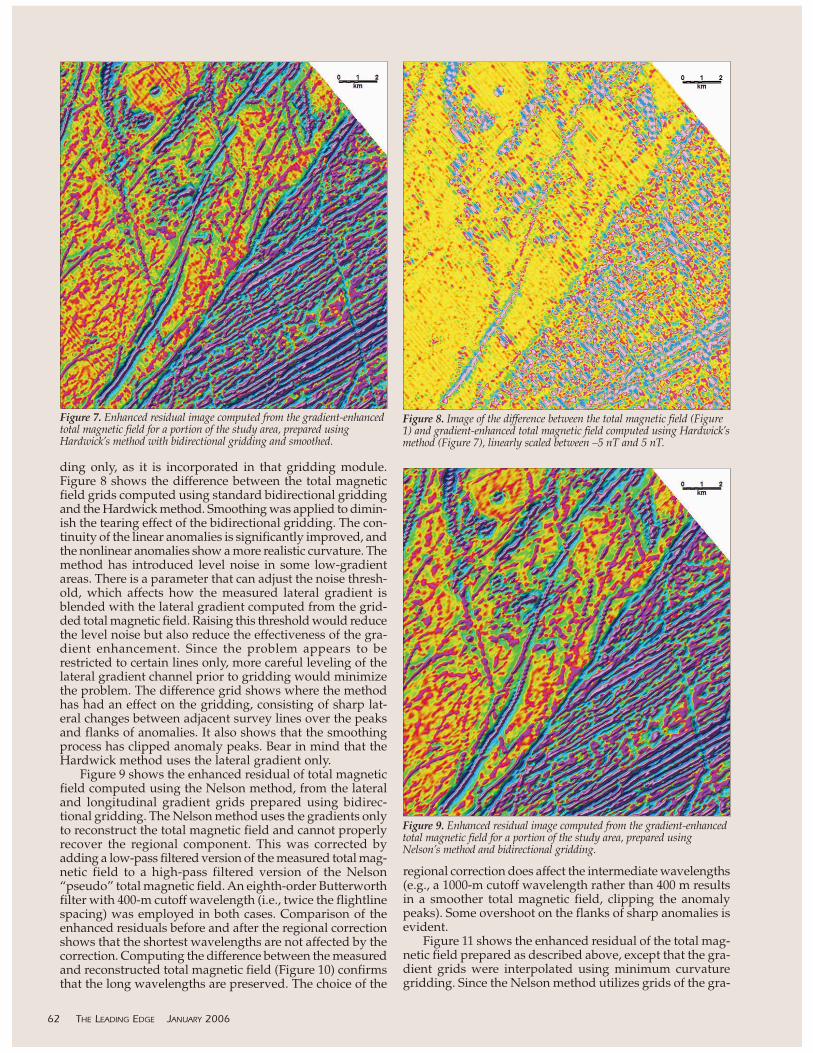
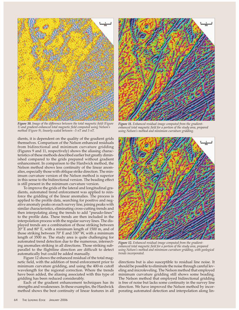
ding only, as it is incorporated in that gridding module.Figure 8 shows the difference between the total magneticfield grids computed using standard bidirectional griddingand the Hardwick method. Smoothing was applied to dimin-ish the tearing effect of the bidirectional gridding. The con-tinuity of the linear anomalies is significantly improved, andthe nonlinear anomalies show a more realistic curvature. Themethod has introduced level noise in some low-gradientareas. There is a parameter that can adjust the noise thresh-old, which affects how the measured lateral gradient isblended with the lateral gradient computed from the grid-ded total magnetic field. Raising this threshold would reducethe level noise but also reduce the effectiveness of the gra-dient enhancement. Since the problem appears to berestricted to certain lines only, more careful leveling of thelateral gradient channel prior to gridding would minimizethe problem. The difference grid shows where the methodhas had an effect on the gridding, consisting of sharp lat-eral changes between adjacent survey lines over the peaksand flanks of anomalies. It also shows that the smoothingprocess has clipped anomaly peaks. Bear in mind that theHardwick method uses the lateral gradient only.

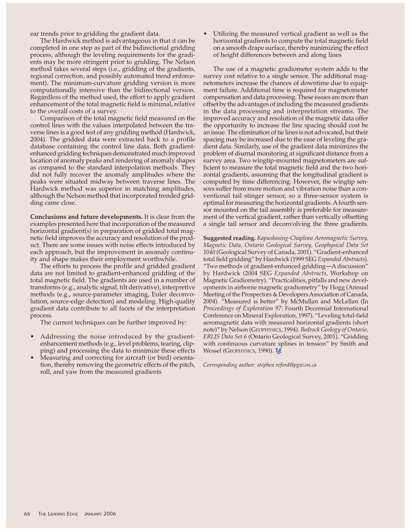
Figure 9 shows the enhanced residual of total magneticfield computed using the Nelson method, from the lateraland longitudinal gradient grids prepared using bidirec-tional gridding. The Nelson method uses the gradients onlyto reconstruct the total magnetic field and cannot properlyrecover the regional component. This was corrected byadding a low-pass filtered version of the measured total mag-netic field to a high-pass filtered version of the Nelson“pseudo” total magnetic field. An eighth-order Butterworthfilter with 400-m cutoff wavelength (i.e., twice the flightlinespacing) was employed in both cases. Comparison of theenhanced residuals before and after the regional correctionshows that the shortest wavelengths are not affected by thecorrection. Computing the difference between the measuredand reconstructed total magnetic field (Figure 10) confirmsthat the long wavelengths are preserved. The choice of the

regional correction does affect the intermediate wavelengths(e.g., a 1000-m cutoff wavelength rather than 400 m resultsin a smoother total magnetic field, clipping the anomalypeaks). Some overshoot on the flanks of sharp anomalies isevident.

Figure 11 shows the enhanced residual of the total mag-netic field prepared as described above, except that the gra-dient grids were interpolated using minimum curvaturegridding. Since the Nelson method utilizes grids of the gra-

62 THE LEADING EDGE JANUARY 2006

Figure 7. Enhanced residual image computed from the gradient-enhancedtotal magnetic field for a portion of the study area, prepared usingHardwick’s method with bidirectional gridding and smoothed.

Figure 8. Image of the difference between the total magnetic field (Figure1) and gradient-enhanced total magnetic field computed using Hardwick’smethod (Figure 7), linearly scaled between –5 nT and 5 nT.

Figure 9. Enhanced residual image computed from the gradient-enhancedtotal magnetic field for a portion of the study area, prepared usingNelson’s method and bidirectional gridding.

dients, it is dependent on the quality of the gradient gridsthemselves. Comparison of the Nelson enhanced residualsfrom bidirectional and minimum curvature gridding(Figures 9 and 11, respectively) shows the aliasing charac-teristics of these methods described earlier but greatly dimin-ished compared to the grids prepared without gradientenhancement. In comparison to the Hardwick method, theNelson method shows less continuity of the linear anom-alies, especially those with oblique strike direction. The min-imum curvature version of the Nelson method is superiorin this sense to the bidirectional version. The beading effectis still present in the minimum curvature version.

To improve the grids of the lateral and longitudinal gra-dients, automated trend enforcement was applied to rein-force the gridding of the linear anomalies. The process isapplied to the profile data, searching for positive and neg-ative anomaly peaks on each survey line, joining peaks withsimilar characteristics, eliminating cross-cutting trends andthen interpolating along the trends to add “pseudo-lines”to the profile data. These trends are then included in theinterpolation process with the regular survey lines. The dis-played trends are a combination of those striking between20� E and 80� E, with a minimum length of 1500 m, and ofthose striking between 70� E and 330� W, with a minimumlength of 3500 m. The study area is quite challenging forautomated trend detection due to the numerous, intersect-ing anomalies striking in all directions. Those striking sub-parallel to the flightline direction are difficult to detectautomatically but could be added manually.

Figure 12 shows the enhanced residual of the total mag-netic field, with the addition of trend enforcement prior tominimum curvature gridding, and using the 400-m cutoffwavelength for the regional correction. Where the trendshave been added, the aliasing associated with this type ofgridding has been reduced considerably.

Each of the gradient enhancement techniques has itsstrengths and weaknesses. In these examples, the Hardwickmethod shows the best continuity of linear features in all

directions but is also susceptible to residual line noise. Itshould be possible to eliminate the noise through careful lev-eling and microleveling. The Nelson method that employedminimum curvature gridding still shows some beading.The Nelson method that employed bidirectional griddingis free of noise but lacks some continuity in the survey linedirection. We have improved the Nelson method by incor-porating automated detection and interpolation along lin-

64 THE LEADING EDGE JANUARY 2006

Figure 10. Image of the difference between the total magnetic field (Figure1) and gradient-enhanced total magnetic field computed using Nelson’smethod (Figure 9), linearly scaled between –5 nT and 5 nT.

Figure 11. Enhanced residual image computed from the gradient-enhanced total magnetic field for a portion of the study area, preparedusing Nelson’s method and minimum curvature gridding.

Figure 12. Enhanced residual image computed from the gradient-enhanced total magnetic field for a portion of the study area, preparedusing Nelson’s method and minimum curvature gridding, with geologicaltrends incorporated.

ear trends prior to gridding the gradient data.The Hardwick method is advantageous in that it can be

completed in one step as part of the bidirectional griddingprocess, although the leveling requirements for the gradi-ents may be more stringent prior to gridding. The Nelsonmethod takes several steps (i.e., gridding of the gradients,regional correction, and possibly automated trend enforce-ment). The minimum-curvature gridding version is morecomputationally intensive than the bidirectional version.Regardless of the method used, the effort to apply gradientenhancement of the total magnetic field is minimal, relativeto the overall costs of a survey.

Comparison of the total magnetic field measured on thecontrol lines with the values interpolated between the tra-verse lines is a good test of any gridding method (Hardwick,2004). The gridded data were extracted back to a profiledatabase containing the control line data. Both gradient-enhanced gridding techniques demonstrated much improvedlocation of anomaly peaks and rendering of anomaly shapesas compared to the standard interpolation methods. Theydid not fully recover the anomaly amplitudes where thepeaks were situated midway between traverse lines. TheHardwick method was superior in matching amplitudes,although the Nelson method that incorporated trended grid-ding came close.

Conclusions and future developments. It is clear from theexamples presented here that incorporation of the measuredhorizontal gradient(s) in preparation of gridded total mag-netic field improves the accuracy and resolution of the prod-uct. There are some issues with noise effects introduced byeach approach, but the improvement in anomaly continu-ity and shape makes their employment worthwhile.

The efforts to process the profile and gridded gradientdata are not limited to gradient-enhanced gridding of thetotal magnetic field. The gradients are used in a number oftransforms (e.g., analytic signal, tilt derivative), interpretivemethods (e.g., source-parameter imaging, Euler deconvo-lution, source-edge detection) and modeling. High-qualitygradient data contribute to all facets of the interpretationprocess.

The current techniques can be further improved by:

• Addressing the noise introduced by the gradient-enhancement methods (e.g., level problems, tearing, clip-ping) and processing the data to minimize these effects

• Measuring and correcting for aircraft (or bird) orienta-tion, thereby removing the geometric effects of the pitch,roll, and yaw from the measured gradients

• Utilizing the measured vertical gradient as well as thehorizontal gradients to compute the total magnetic fieldon a smooth drape surface, thereby minimizing the effectof height differences between and along lines

The use of a magnetic gradiometer system adds to thesurvey cost relative to a single sensor. The additional mag-netometers increase the chances of downtime due to equip-ment failure. Additional time is required for magnetometercompensation and data processing. These issues are more thanoffset by the advantages of including the measured gradientsin the data processing and interpretation streams. Theimproved accuracy and resolution of the magnetic data offerthe opportunity to increase the line spacing should cost bean issue. The elimination of tie lines is not advocated, but theirspacing may be increased due to the ease of leveling the gra-dient data. Similarly, use of the gradient data minimizes theproblem of diurnal monitoring at significant distance from asurvey area. Two wingtip-mounted magnetometers are suf-ficient to measure the total magnetic field and the two hori-zontal gradients, assuming that the longitudinal gradient iscomputed by time differencing. However, the wingtip sen-sors suffer from more motion and vibration noise than a con-ventional tail stinger sensor, so a three-sensor system isoptimal for measuring the horizontal gradients. Afourth sen-sor mounted on the tail assembly is preferable for measure-ment of the vertical gradient, rather than vertically offsettinga single tail sensor and deconvolving the three gradients.

Suggested reading. Kapuskasing-Chapleau Aeromagnetic Survey,Magnetic Data, Ontario Geological Survey, Geophysical Data Set1040 (Geological Survey of Canada, 2001). “Gradient-enhancedtotal field gridding” by Hardwick (1999 SEG Expanded Abstracts).“Two methods of gradient-enhanced gridding—A discussion”by Hardwick (2004 SEG Expanded Abstracts, Workshop onMagnetic Gradiometry). “Practicalities, pitfalls and new devel-opments in airborne magnetic gradiometry” by Hogg (AnnualMeeting of the Prospectors & Developers Association of Canada,2004). “Measured is better” by McMullan and McLellan (InProceedings of Exploration 97: Fourth Decennial InternationalConference on Mineral Exploration, 1997). “Leveling total-fieldaeromagnetic data with measured horizontal gradients (shortnote)” by Nelson (GEOPHYSICS, 1994). Bedrock Geology of Ontario,ERLIS Data Set 6 (Ontario Geological Survey, 2001). “Griddingwith continuous curvature splines in tension” by Smith andWessel (GEOPHYSICS, 1990). TLE

Corresponding author: stephen.reford@pgw.on.ca

66 THE LEADING EDGE JANUARY 2006