FACULTAD DE CIENCIAS ECONÓMICAS

Y EMPRESARIALES

GRADO EN ECONOMÍA

Is the Forward Rate a True Unbiased Predictor of the Future Spot Exchange Rate?

Autor: Elena Renedo Sánchez

Tutor: Juan Ángel Jiménez Martín

Curso Académico 2012/2013

27 de mayo de 2013

1

Is the Forward Rate a True Unbiased Predictor of the Future Spot Exchange

Rate?

ABSTRACT

In the past decades, there have been many empirical studies both in support

of or opposing the Forward Rate Unbiasedness Hypothesis. This hypothesis

argues that the forward rate fully reflects the information regarding exchange

rate expectations and so, forward premiums predicts the direction change in

future spot rates. In this paper we examine monthly data on spot and one-

month forward prices for the yen, the euro and the sterling pound, all relative to

the USD. Our purpose is to study the relationship between forward rates and

future spot rates before and after the beginning of the Global Financial Crisis of

September 2008, by testing if the forward rate is an unbiased estimator of the

future spot rate. To test this hypothesis the conventional method is followed, by

using an OLS regression with the change in spot exchange rate as the

dependent variable, while the forward premium as the independent variable. To

support this hypothesis, the constant term would not differ from zero, the

coefficient of the forward premium would not significantly differ from one and the

error term would not exhibit any serial correlation. At the end, we conclude that

forward exchange rates have little effect as forecasts of future spot exchange

rates since the Forward Rate Unbiasedness Hypothesis is rejected.

2

Contents

1. INTRODUCTION ..................................................................................................... 3

2. SOME FACTS ABOUT THE FOREIGN EXCHANGE MARKET........................ 5

3. THEORETICAL REVIEW ....................................................................................... 6

4. METHODOLOGY .................................................................................................. 10

5. RESULTS................................................................................................................ 13

5.1. DESCRIPTIVE STATISTICS ....................................................................... 13

5.2. UNIT ROOT TESTS...................................................................................... 16

5.3. AUTOCORRELATION AND HETEROCEDASTICITY ANALYSIS ....... 19

5.4. REGRESSION TEST ...................................................................................... 20

6. CONCLUSION ....................................................................................................... 25

6. REFERENCES ........................................................................................................ 26

3

1. INTRODUCTION

This paper reviews the Forward Rate Unbiasedness Hypothesis which states

that forward rate is equal to the conditional expectation of the future spot

exchange rate under the assumptions of rational expectations and risk

neutrality. The main purpose of this study is to conclude if the former can be

considered as an unbiased predictor for the latter or on the contrary, the

Forward Rate Unbiasedness Hypothesis must be rejected.

The study of the relationship between the forward and the corresponding future

spot rate and how exchange rates are determined are of great concern for

individual investors and policy makers. In fact, exchange rate is one of the most

determinant factors in a country because it links the domestic economy to the

rest-of-world economy. Hence, the exchange rate strongly influences the

competitiveness of commodities’ markets and final allocation of resources.

An appreciation of a currency raises the price of domestic goods relative to the

price of foreign goods. As a result, domestic exports became less competitive in

world markets, and import substitution goods became less competitive in the

national country. Alternatively, home currency depreciation results in a more

competitive traded goods sector, stimulating domestic employment and

inducing a shift in resources from the non traded-to the traded-goods sector.

The bad part is that currency weakness also results in higher prices for

imported goods and services, worsening living standards and domestic inflation.

In that sense, it is important to analyze the movements experienced by the

exchanges rates of the main currencies and their effects on the current Global

Financial Crisis. One of the main characteristics showed by the World Economy

with the beginning of the crisis and the fall of Lehman Brothers in September

2008, was the existence of large external deficits in some countries, like the

U.S., and surpluses in others, as in China. This global disequilibrium is the

result of several factors and one of the fundamental ones are the exchange

rates.

There has always been external disequilibrium, but never in history with the

magnitude of recent years. So, the evolution of exchange rates and the

currency prices will determine the adjustment of these global economic

imbalances and to a large extent, the recovery of production and the most

important consequence, the creation employment.

To test the Forward Rate Unbiasedness Hypothesis and analyze the

fluctuations produced in the exchange rates, the conventional method was

followed, which implies the use of an OLS regression, with the variation in spot

4

exchange rate (St+1 –St) as the explained variable, while the forward premium

(Ft-St) as explanatory one. We conclude that the Unbiasedness hypothesis

cannot be demonstrated and so, forward rates have little effect as forecasts of

future spot exchange rates.

The present paper is organized as follows. Section 2 provides information about

the main stylized facts of the Foreign Exchange Market. Then, section 3

addresses a theoretical background about exchange rates determination and it

reviews previous studies regarding the possible validity of the forward rate as

an unbiased predictor. Section 4 deals with the methodology of the regression

model used for this research. Next, section 5 reports the results from the

regression analysis, after the model was corrected for serial correlation and

heteroscedasticity. Finally, section 6 summarizes all the conclusions derived

from our study.

5

2. SOME FACTS ABOUT THE FOREIGN EXCHANGE MARKET

The Foreign Exchange Market, also called the “Forex” is the most liquid

financial market in the world. Nowadays, since currencies are the main

regulation mechanism for individuals’ interactions in an economy, it is important

to understand how their values are determined.

Currencies have increasingly become one of the more actively traded assets

and so, the volume and speed of their flows are just amazing. Approximately,

average daily turnover in global foreign exchange markets is estimated at $3.98

trillion. The $3.98 trillion break-down is as follows. Approximately, $1.490 trillion

in spot transactions, $475 billion in outright forwards and $1.765 trillion in

foreign exchange swaps. The rest, around $250 billion are divided into currency

swaps, options and other products. Besides, the major currencies which are

traded in the Forex are U.S dollar, the Euro, the Japanese Yen and also, the

Sterling Pound.

There is not just a unified or centrally established market for the majority of

trades. Due to the over-the-counter (OTC) nature of currency markets, there are

rather a many interconnected marketplaces, where different currencies

instruments are negotiated. For that reason, there is not a single exchange rate

but rather a number of different rates or prices depending on which bank or

investor is trading and the location of this one.

In that sense, the main trading centers are New York and London,

although Tokyo, Hong Kong and Singapore are important as well. Currency

trading happens continuously throughout the day, so when the Asian trading

session ends, the European session begins, followed by the North American

session and then coming back again to the Asian session.

6

3. THEORETICAL REVIEW

This section provides a theoretical literature review in order to understand how

the forecasting of future spot exchange rates works and also, the conditions

under which the Forward Rate Unbiasedness Hypothesis is satisfied.

Our purpose is to derive the Unbiasedness Hypothesis by following both the

theoretical reasoning of the Covered and Uncovered Rate Parity Conditions.

The Covered Interest Parity is considered as the no-arbitrage condition in

foreign exchange markets. Concretely, it implies a situation in where the

relationship between interest rates and the spot and forward currency values of

two countries are in equilibrium. As a result, there are no interest rate arbitrage

opportunities between those two currencies.

In this sense, the Covered Interest Parity (CIP) represents a condition under

which investors are not exposed to a foreign exchange risk by means of the use

of a forward contract, so the exchange rate risk is effectively covered. Under this

condition, a domestic investor would earn equal returns from investing in

domestic assets or converting currency at the spot exchange rate, investing in

foreign currency assets, and exchanging the foreign currency for domestic

currency at the negotiated forward rate. Investors will be indifferent to the

interest rates on deposits in these countries due to the equilibrium resulting

from the forward exchange rate. The condition allows for no arbitrage

opportunities because the return on domestic deposits d is equal to the

return on foreign deposits

f .

The following equation reflects the concept of this CIP:

d

f (1)

Rearranging the previous equation and solving for , what we obtain is:

(2)

Equation (2) which results from the relationship between forward and spot

exchange rates within the context of CIP is responsible for avoiding arbitrage

strategies and so, potential opportunities to obtain profits. However, in order for

this equilibrium to hold under differences in interest rates between two

countries, the forward exchange rate must generally differ from the spot

7

exchange rate, such that a no-arbitrage condition is sustained. Therefore, the

forward rate is said to contain a premium or discount, reflecting the interest rate

differential between two countries.

The forward exchange rate differs by a premium or discount of the spot

exchange rate:

(3)

Where P is the premium or discount.

Equation (3) can be rearranged as follows in order to solve for the forward

premium/discount:

(4)

On the contrary, when the no-arbitrage condition is satisfied without the use of a

forward contract to hedge against exposure to exchange rate risk, interest rate

parity is said to be uncovered and so, we arrive to the Uncovered Interest Parity

(UIP). In this situation, risk-neutral investors will be indifferent among the

available interest rates in two countries because the exchange rate between

those countries is expected to adjust such that the domestic return on domestic

deposits is equal to the domestic return on foreign deposits, thereby eliminating

the potential for uncovered interest arbitrage profits.

The following equation represents the Uncovered Interest Parity condition:

d t t+k t f) (5)

Now, we are going to demonstrate that if we combine both conditions, so that

both Covered and Uncovered Interest Parity hold, we can derive an important

relationship between the forward and expected future spot exchange rates:

CIP: d

f) (6)

UIP: d t t+k t f) (7)

Dividing UIP between CIP yields the following equation:

8

t t+k t (8)

Equation (8) can be rewritten and solved for Ft, so that:

t t t+k) (9)

t is the forward exchange rate at t

t t+k is the expected future spot rate at t+k, where k is the number of

periods into the future from time t

This last expression represents the Unbiasedness Forward Rate Hypothesis,

suggesting that the forward rate it can be assumed as an unbiased predictor of

the future spot rate.

Up to our days, economists have found empirical evidence that CIP generally

holds, although not in a completely accurate way. In that sense, the Forward

Rate Unbiasedness Hypothesis can serve as a test to determine whether UIP

holds, so in order for the forward rate to reflect the true spot rate value, both

CIP and UIP conditions must hold.

The Unbiasedness Hypothesis states that under conditions of rational

expectations and risk neutrality, the forward exchange rate is an unbiased

estimator of the future spot exchange rate. This Unbiasedness Hypothesis is a

key puzzle among economists and financial researchers. In general, the

majority of recent studies regarding the Unbiasedness Forward Rate

Hypothesis have empirically demonstrated the inability of the forward rate to be

an unbiased and good predictor for the future spot rate.

Nowadays, there exists an enormous literature available on whether the forward

exchange rate is an unbiased predictor of the future spot exchange rate. Due to

the vast nature of the literature present in the field, we only refer to some

important works in this paper.

Eugene Fama (1984) considered that forward rate could be interpreted as the

sum of a premium and the expected future spot rate. More precisely, “The

forward exchange rate ft observed for an exchange at time t+1 is the market

determined certainty equivalent of the future exchange rate st+1

“1

1 Fama, Eugene. (1984). Forward and Spot Exchanges Rates.

9

Fama conducted a study testing a model for measurement of both variation in

the premium and the expected future spot rate components of forward rates.

Assuming that the forward market is efficient or rational, the study found

evidence that both components of forward rates vary through time. In fact, the

study has two important conclusions. The first is that the premium and the

expected future spot rate components of forward rates are negatively

correlated. The second one it was that most of the variation in forward rates is

due to the variation in the premiums.

Besides, Thomas Chiang (1988) conducted a study developing a stochastic

coefficient model to examine the unbiased forward rate hypothesis proposing

that “with effective use of information underlying the stochastic pattern of the

estimated parameters in forecasting, it is possible to improve the accuracy of

the exchange rate predictions”2.

However, his study also considers that through the use of Brown-Durbin-Evans

test and the Chow test, the constant coefficient hypothesis cannot be

supported. He found that the constant term and the coefficient for the one-

period lagged forward rate are subject to newly available information and vary

through the sub-sample periods that he tested. Specifically, he realized that

when he tested sub-samples, in many cases, the constant term was

significantly different from zero and the coefficient of one-period lagged forward

rate was significantly different from one. Another interesting aspect of Chiang’s

study is that he added the two-period lagged forward rate as independent

variable in predicting the spot rate and this variable was not found to be

significant at the 5% level, suggesting that it contains no significant contribution

to the explanation for the spot rate.

2 Chiang, Thomas C. (1988). The Forward Rate as a Predictor of the Future Spot Rate. A

Stochastic Coefficient Approach.

10

4. METHODOLOGY

In this section, we provide the methodology that leads us to conclude that regression (10) is the better one we can use to analyze the validity or invalidity of the Forward Rate Unbiasedness Hypothesis.

t+k – t i i t - t i,t+k (10)

where the change in spot exchange rate is the dependent variable and the

forward premium is independent variable.

Under conditions of risk neutrality and rational expectations on the part of

market agents, the forward rate is an unbiased predictor of the corresponding

future spot rate. Assuming the absence of risk premium in the foreign exchange

market it must holds true that

t t+k t (11)

Where t is the log forward rate at time t for delivery k periods later, St+k is the

corresponding log spot rate at time t +k, and t t+k is the mathematical

expectations operator conditioned on the information set available at time t.

Assuming the formation of rational expectations, as Muth (1960) stated,

“expectations are essentially the same as the predictions of the relevant

economic theory."3

t+k= t( t+k t+k (12)

Where t+k, the rational expectations realized forecast error, must have a

conditional expected value of zero and be uncorrelated with any information

available at time t.

However, as time went on Fama (1984) deepened in this analysis regarding the

price determination on future markets. He stated that correct analysis will be the

one in which t observed at time t for an exchange at time t +k, reflects the

future variation of the future spot exchange rate t+k. Besides, Fama considered

that the forward rate could be divided into an expected future spot rate t( t+k)

and premium (Pt) so that,

t t+k t (13)

3 Muth, John F.(1961). Rational Expectations and the Theory of Price Movements.

11

Note that t = t, t+k = t+k and that, the expected future spot rate t+k is

the rational forecast, derive from all the information of period t. In that sense,

the idea behind using logs is basically in order to make easier our analysis. This

implies that our analysis is independent on whether we use one or another

currency.

Following the methodology established by Fama, from (13) if we subtract t on

both sides of the equation, we observe that the difference between the forward

rate and the current spot rate is defined as:

t t t t+k t (14)

Which reflects that forward premium ( t t) will be determined by the risk

premium of the market ( t) and the expected variation in spot exchanges rates

t+k t).

Then, focusing on the main target, the study of the Forward Rate Unbiasedness

Hypothesis, that is, trying to figure out if the forward premium really predict the

future spot rate, Fama proposed two different regression models. What changes

in each one of them is the dependent variable, which are Ft – S t+k and S t+k – St

(both observed at t+k), while the independent variable is the same for the both

of them, Ft – St (observed at t). What we obtain are the following equations, (15)

and (16):

t t+k 1 1 t t 1,t+k (15)

St+k– St 2 2 t t + 2,t+k (16)

In this way, estimates of (16) tell us whether the current forward-spot differential

or forward premium, t t+k , has power to predict the future change in spot

rate, St+k – St. Evidence that 2 is reliably non-zero means that the forward rate

observed at t has information about the spot rate to be observed at t+k.

Likewise, since t t+k is the premium t plus t+k t) (see equation 14), the

random error of the rational forecast t+k evidence that 1 in (15) is reliably

non-zero means that the premium component of t t has variation that shows

up reliably in t t+k.

Since t t+k and St+k– St sum to t t, the sum of the intercepts in (15) and (16)

must be zero, the sum of the slopes must be 1 and the disturbances period by

period must sum 0. In other words, what Fama said is that both regressions (15)

12

and (16) contain identical information about the variation of the t and

t+k t) components of t t.

In this sense, Fama suggested that considering a joint analysis of the two

regressions is what will reflect clearly the information that either contains.

However, for our analysis we are going to choose the second, equation (16). In

fact, as Fama concludes regression (16) become more common in financial

literature and so, it has seemed to be more efficient in telling us whether the

current forward-spot differential or forward premium, t t has a power to

predict the future change in the spot rate, S t+k – St .

Finally, just to be as much precise as possible, it is important to know that

earliest studies in the 1970s dealt with a simple regression of the future spot

exchange rate (St+k) on the current forward exchange rate (Ft) with an error

term with a conditional mean of zero [Et(ut+k)].

t+k i i t i,t+k (17)

However, this regression model was found to be incorrect as both the forward

and the spot rates were shown to be non-stationary series, they were integrated

of order one. Subsequently, to resolve this problem, the model was modified

and the Forward Rate Unbiasedness Hypothesis was tested by running the

regression of the change in the future spot exchange rate ( t+k – t) on the

forward premium ( t - t).

In such a way, as we announced previously, the standard test to determine

whether the forward rate is an unbiased efficient predictor of future spot rates,

has become to run a regression as (18):

t+k – t i t - t i,t+k (18)

If t was an unbiased, efficient predictor of t+k then :

i i

13

5. RESULTS

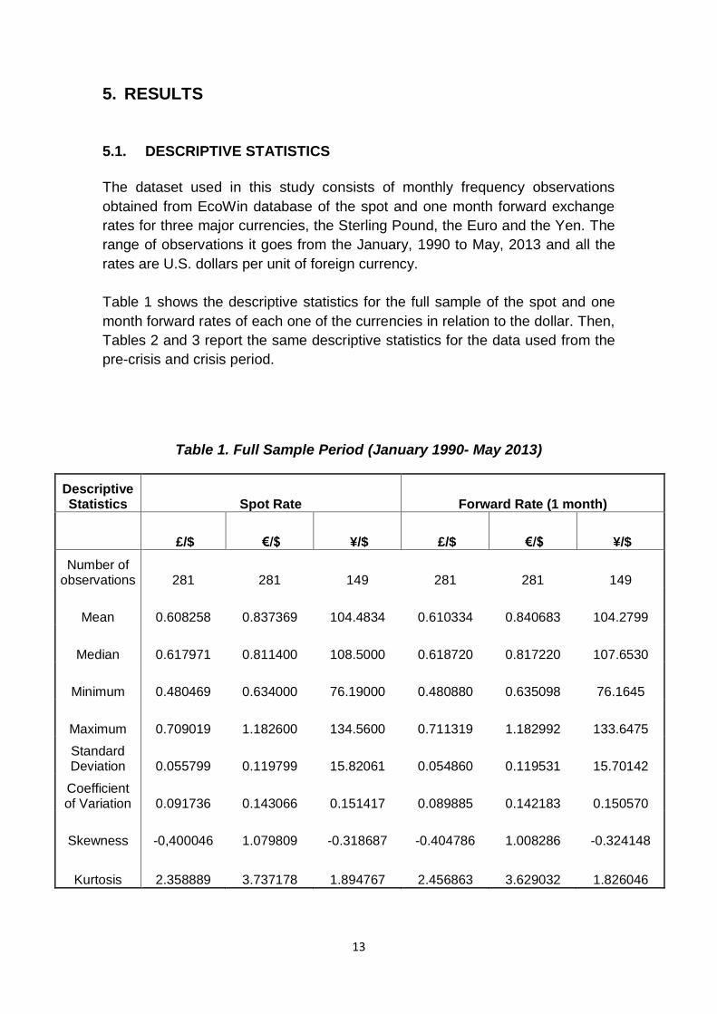
5.1. DESCRIPTIVE STATISTICS

The dataset used in this study consists of monthly frequency observations

obtained from EcoWin database of the spot and one month forward exchange

rates for three major currencies, the Sterling Pound, the Euro and the Yen. The

range of observations it goes from the January, 1990 to May, 2013 and all the

rates are U.S. dollars per unit of foreign currency.

Table 1 shows the descriptive statistics for the full sample of the spot and one

month forward rates of each one of the currencies in relation to the dollar. Then,

Tables 2 and 3 report the same descriptive statistics for the data used from the

pre-crisis and crisis period.

Table 1. Full Sample Period (January 1990- May 2013)

Descriptive Statistics Spot Rate Forward Rate (1 month)

£/$ €/$ ¥/$ £/$ €/$ ¥/$

Number of observations 281 281 149 281 281 149

Mean 0.608258 0.837369 104.4834 0.610334 0.840683 104.2799

Median 0.617971 0.811400 108.5000 0.618720 0.817220 107.6530

Minimum 0.480469 0.634000 76.19000 0.480880 0.635098 76.1645

Maximum 0.709019 1.182600 134.5600 0.711319 1.182992 133.6475

Standard Deviation 0.055799 0.119799 15.82061 0.054860 0.119531 15.70142

Coefficient of Variation 0.091736 0.143066 0.151417 0.089885 0.142183 0.150570

Skewness -0,400046 1.079809 -0.318687 -0.404786 1.008286 -0.324148

Kurtosis 2.358889 3.737178 1.894767 2.456863 3.629032 1.826046

14

Table 2. Pre-crisis Period (January 1990- August 2008)

Descriptive Statistics Spot Rate Forward Rate (1 month)

£/$ €/$ ¥/$ £/$ €/$ ¥/$

Number of observations 224 224 92 224 224 92

Mean 0.601416 0.860975 115.4004 0.603999 0.865129 115.4517

Median 0.609663 0.829000 116.6350 0.611076 0.835596 116.4517

Minimum 0.480469 0.634000 99.81000 0.480880 0.635098 99.54430

Maximum 0.709019 1.182600 134.5600 0.711319 1.182992 133.6475

Standard Deviation 0.059184 0.121991 7.441914 0.058339 0.120839 7.371949

Coefficient of Variation 0.098408 0.141689 0.064788 0.096588 0.139677 0.064038

Skewness -0.173537 0.867127 0.205585 -0.190320 0.800594 0.155371

Kurtosis 2.055174 3.286178 2.810310 2.139034 3.259795 2.739126

15

Table 3. Crisis Period (September 2008- May2013)

Descriptive Statistics Spot Rate Forward Rate (1 month)

£/$ €/$ ¥/$ £/$ €/$ ¥/$

Number of observations 57 57 57 57 57 57

Mean 0.635147 0.744602 86.86281 0.635280 0.744615 86.78592

Median 0.630358 0.749500 86.34000 0.630354 0.749372 86.32470

Minimum 0.560150 0.666400 76.19000 0.559616 0.666427 76.16450

Maximum 0.698861 0.817400 106.0300 0.699012 0.817220 105.4406

Standard Deviation 0.026383 0.038551 7.724072 0.026471 0.038801 7.664199

Coefficient of Variation 0.041538 0.051774 0.088923 0.041668 0.052109 0.883115

Skewness 0.423658 0.090530 0.386450 0.405172 -0.085193 0.365928

Kurtosis 3.669874 2.0993539 2.073365 3.731931 2.088576 2.026869

It can be appreciated that the three currencies have experienced a depreciation trend from the beginning of the crisis in September 2008 with the fall of Lehman Brothers. The mean reflected in table 3 for both spot and forward rates are lower than those in table 2, except for the case of the British Pound. Both the euro/dollar and yen/dollar exchange rate parity have declined during the crisis, whereas the British Pound showed a higher value of the mean for the Crisis period than for the Pre-Crisis one. This fact could reflect that both the Euro and the Yen are increasingly losing their value and so, they are weaker now than before. Besides, there is another interesting point here. The volatility of exchanges rates which are measured by the standard deviation and the coefficient of variation are lower in table 3 than in table 2. Initially, we could expect just the opposite. However, one reason which could explain the higher volatility in table 2 is that for this Pre-Crisis period we have included year 2007 and 2008 up to September. In fact, although for this paper we consider the beginning of the Crisis with the fall of Lehman Brothers in September 2008, all the studies and economic research suggest that crisis effects appeared in the summer of 2007.

16

In such a way, the contrast between the higher values of the exchange rates in the 90’s with those of 2007 and 2008 which are lower for all the currencies, could explain this greater volatility in table 2 than in table 3. Regarding table 1, which included the full sample period (1990-2013), we can observe that all values are intermediate with respect to those showed in tables 2 and 3 for the Pre-Crisis and Crisis periods, which seems to be very reasonable because it includes both subsamples.

5.2. UNIT ROOT TESTS

One important assumption of the Unbiased Forward Hypothesis is that the

forward and spot rates are stationary. More sophisticated techniques in

econometrics have shown that macroeconomic time series in their levels are

non-stationary and hence their variances tend to increase with time.

In fact, non-stationarity of time series is regarded as a problem in econometric

analysis. A series is said to be (weakly or covariance) stationary if the mean

and the autocovariances of the series do not depend on time.

A common example of non-stationary series is the random walk:

t t-1 t (19)

Where is a stationary random disturbance term. The series has a constant

forecast value, conditional on t, and the variance is increasing over the time.

The random walk is a difference stationary series since the first difference of

is stationary.

t- t-1 t t (20)

A difference stationary series is said to be integrated and is denoted as I(d)

where d is the order of integration. The order of integration is the number of unit

roots contained in the series, or the number of differencing operations it takes to

makes the series stationary. For the random walk above, there is one unit root

test, so it is an I(1) series. Similarly, a stationary series is I(0).

Standard inference procedures do not apply to regressions which contain an

integrated dependent variable or integrated regressors. Therefore, it is

important to check whether a series is stationary or not before using it in a

regression. The formal method to test the stationarity of a series is the unit root

test.

17

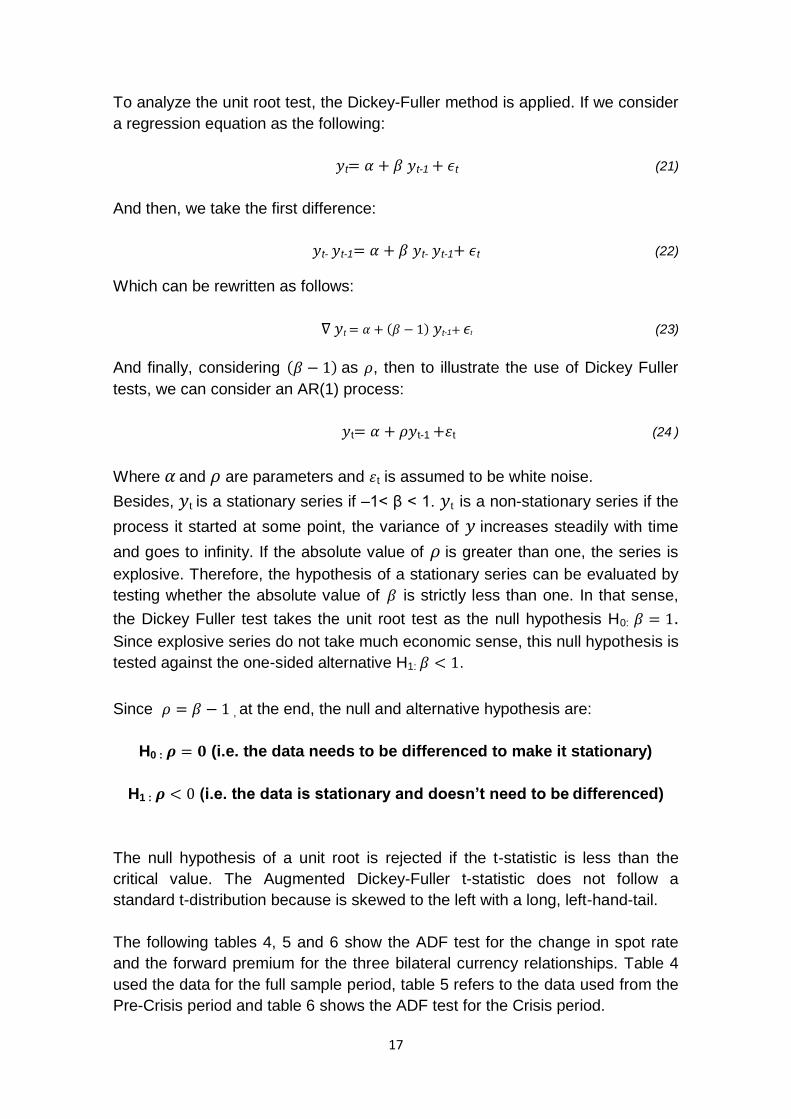
To analyze the unit root test, the Dickey-Fuller method is applied. If we consider

a regression equation as the following:

t t-1 t (21)

And then, we take the first difference:

t- t-1 t- t-1 t (22)

Which can be rewritten as follows:

t t-1 t (23)

And finally, considering as , then to illustrate the use of Dickey Fuller

tests, we can consider an AR(1) process:

t t-1 t (24 )

Where and are parameters and t is assumed to be white noise.

Besides, t is a stationary series if –1< β < 1. t is a non-stationary series if the

process it started at some point, the variance of increases steadily with time

and goes to infinity. If the absolute value of is greater than one, the series is

explosive. Therefore, the hypothesis of a stationary series can be evaluated by

testing whether the absolute value of is strictly less than one. In that sense,

the Dickey Fuller test takes the unit root test as the null hypothesis H0: .

Since explosive series do not take much economic sense, this null hypothesis is

tested against the one-sided alternative H1: .

Since , at the end, the null and alternative hypothesis are:

H0 : (i.e. the data needs to be differenced to make it stationary)

H1 : (i.e. the data is stationary and doesn’t need to be differenced)

The null hypothesis of a unit root is rejected if the t-statistic is less than the

critical value. The Augmented Dickey-Fuller t-statistic does not follow a

standard t-distribution because is skewed to the left with a long, left-hand-tail.

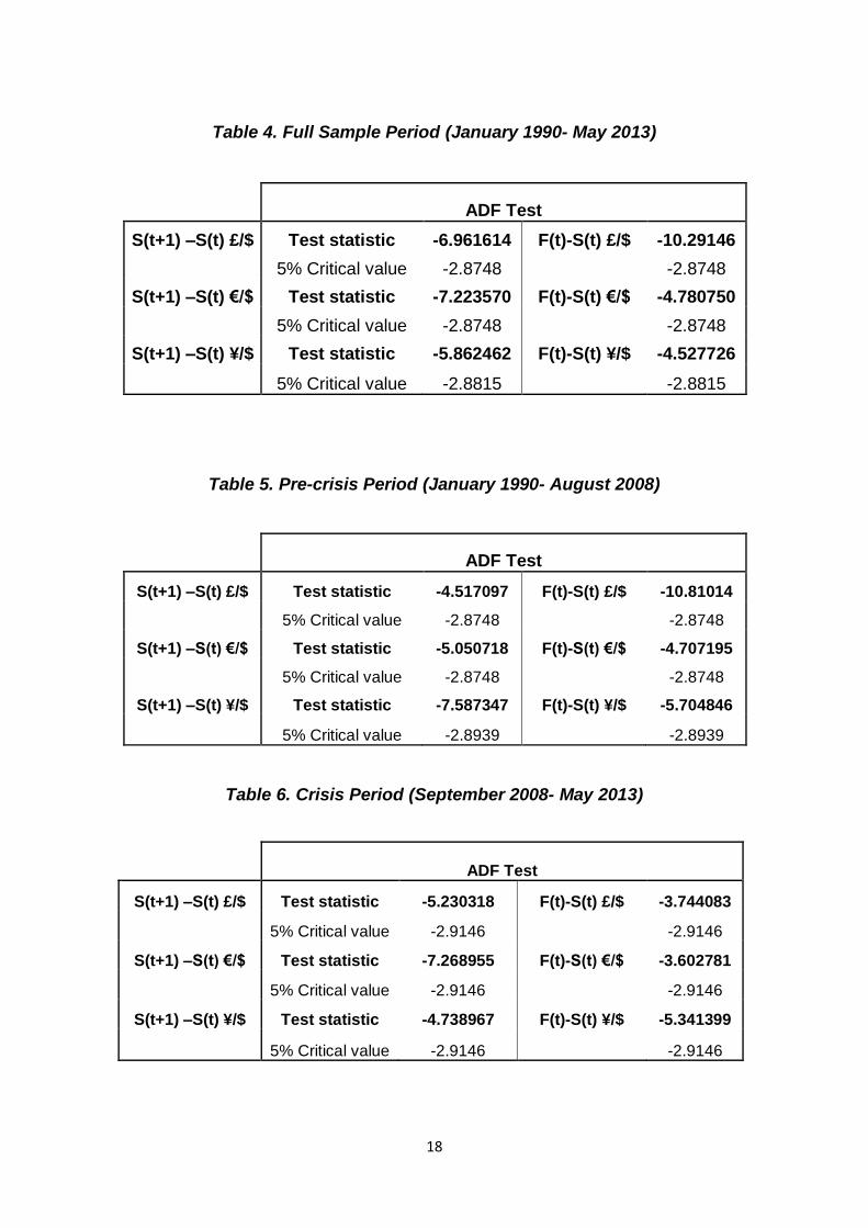
The following tables 4, 5 and 6 show the ADF test for the change in spot rate

and the forward premium for the three bilateral currency relationships. Table 4

used the data for the full sample period, table 5 refers to the data used from the

Pre-Crisis period and table 6 shows the ADF test for the Crisis period.

18

Table 4. Full Sample Period (January 1990- May 2013)

ADF Test

S(t+1) –S(t) £/$ Test statistic -6.961614 F(t)-S(t) £/$ -10.29146

5% Critical value -2.8748 -2.8748

S(t+1) –S(t) €/$ Test statistic -7.223570 F(t)-S(t) €/$ -4.780750

5% Critical value -2.8748 -2.8748

S(t+1) –S(t) ¥/$ Test statistic -5.862462 F(t)-S(t) ¥/$ -4.527726

5% Critical value -2.8815 -2.8815

Table 5. Pre-crisis Period (January 1990- August 2008)

ADF Test

S(t+1) –S(t) £/$ Test statistic -4.517097 F(t)-S(t) £/$ -10.81014

5% Critical value -2.8748 -2.8748

S(t+1) –S(t) €/$ Test statistic -5.050718 F(t)-S(t) €/$ -4.707195

5% Critical value -2.8748 -2.8748

S(t+1) –S(t) ¥/$ Test statistic -7.587347 F(t)-S(t) ¥/$ -5.704846

5% Critical value -2.8939 -2.8939

Table 6. Crisis Period (September 2008- May 2013)

ADF Test

S(t+1) –S(t) £/$ Test statistic -5.230318 F(t)-S(t) £/$ -3.744083

5% Critical value -2.9146

-2.9146

S(t+1) –S(t) €/$ Test statistic -7.268955 F(t)-S(t) €/$ -3.602781

5% Critical value -2.9146

-2.9146

S(t+1) –S(t) ¥/$ Test statistic -4.738967 F(t)-S(t) ¥/$ -5.341399

5% Critical value -2.9146 -2.9146

19

5.3. AUTOCORRELATION AND HETEROCEDASTICITY ANALYSIS

Before analyzing the results obtained for the OLS regression test, it is important

to check that our variables do not present serial correlation. In regression

analysis for time series data, autocorrelation of the errors is a problem.

Autocorrelation of the errors, which themselves are unobserved, can generally

be detected since it produces autocorrelation in the observed residuals. In fact,

autocorrelation violates the OLS assumption that the error terms are

uncorrelated. While it does not bias the OLS coefficient estimates, the standard

errors tend to be underestimated when the autocorrelations of the errors at low

lags are positive.

The traditional test for the presence of first-order autocorrelation is the Durbin–

Watson statistic, which if lower than 2, it implies a positive autocorrelation

between variables.

In this case, when we initially compute the regression for each one of the

currencies with respect to the dollar, for the Full Sample, the Pre-Crisis and the

Crisis periods, all the Durbin Watson obtained were lower than 2. In order to fix

the serial correlation, an autoregressive term AR(1) is going to be included for

all the regression equations. In fact, the AR(1) term is going to be significant

and the Durbin Watson statistic closed to 2.

Otherwise, we could have used another method to detect the existence of

autocorrelation just by looking at the residual graph. In this sense, if positive

errors are followed by positive and negative errors of the same size, then we

are in the presence of positive autocorrelation.

Regarding the variability of the variables it is important to detect if they exhibit a

constant variance (homoscedasticity) or not (heteroscedasticity).

This fact is also a major concern for the latter application of regression analysis

because the presence of heterocedasticity can invalidate statistical test of

significance which assumes that the modeling errors are uncorrelated, normally

distributed and their variance does not vary with the effects being modeled.

For all of the cases, it can be observed the existence of heterocedasticity. In

that sense, we apply HAC Consistent Covariances (Newey-West) that is

consistent in the presence of heterocedasticity and autocorrelation.

Finally, in order to determinate if the unbiased forward rate hypothesis is fulfilled

or not, we will proceed to the regression analysis of the equations considered in

this study. We will try to answer to the crucial question focusing on whether or

not the forward premiums it contains so valuable information that can be used

to predict the future fluctuation of the spot exchange rates. Besides, we will

20

analyze the results from the following regressions in order to determinate how

exchanges rates have behaved before and after the beginning of the Great

Financial Crisis.

5.4. REGRESSION TEST

As we already mention, this study examines the effectiveness of the forward

premium (Ft-St) in determining the future spot exchange rate (St+1-St) in order to

conclude whether the Forward Rate Unbiasedness hypothesis is fulfilled or not.

The regression used is:

t+1 – t t - t 1,t+1 (25)

Ordinary Least Squares Method (OLS) is used, which ensures that the

coefficients will be best linear unbiased estimators (BLUE).

Tables 7, 8 and 9 summarize all the regressions considered for this study,

which are computed for the three different exchange rates relationships (£/$,

€/$ and ¥/$) for the Full Sample, the Pre-Crisis and Crisis periods.

Table 7.Full Sample Period (January 1990- May 2013)

Equation Source Exchange

Rate Horizon Frequency Time

Period No. Of observations

1 EcoWin £/$ 1 month Monthly 1990-2013 281

2 EcoWin €/$ 1 month Monthly 1990-2013 281

3 EcoWin ¥/$ 1 month Monthly 2001-2013 149

21

Table 8.Pre-Crisis Period (January 1990- August 2008)

Equation Source Exchange

Rate Horizon Frequency Time

Period No. Of observations

1 EcoWin £/$ 1 month Monthly 1990-2008 224

2 EcoWin €/$ 1 month Monthly 1990-2008 224

3 EcoWin ¥/$ 1 month Monthly 2001-2008 92

Table 9. Crisis Period (September 2008- May 2013)

Equation Source Exchange

Rate Horizon Frequency Time

Period No. Of observations

1 EcoWin £/$ 1 month Monthly 2008-2013 57

2 EcoWin €/$ 1 month Monthly 2008-2013 57

3 EcoWin ¥/$ 1 month Monthly 2008-2013 57

The results of these OLS regressions are contained in tables 10, 11 and 12.

Since we are analyzing the unbiasedness of the one-month forward exchange

rate, the value of k in the regression model is equal to 1. The following tables

22

show the results obtained for the coefficients; the constant terms ( ); the

adjusted determination coefficient (R2) and the Durbin Watson Statistic (DW).

Table 10. Full Sample Period (January 1990- May 2013)

Exchange Rate Parity R2 DW

£/$

-0.001633 (0.231808)

-0.677551*

(0.287256) 0.071049 1.719260

€/$ -0.000732 (0.221849)

-0.770551**

(0.302178) 0.054020 1.864846

¥/$ 0.000684

(0.296368) -1.017553*

(0.312556) 0.039576 1.801432

** Significant at 1%

* Significant at 5%

Standard errors are indicates in parentheses

Table 11. Pre-Crisis Period (January 1990- August 2013)

Exchange Rate Parity R2 DW

£/$ -0.003601*

(0.221510) -0.747418*

(0.237407) 0.050952 1.928035

€/$ -0.001609*

(0.212125) -0.767829** (0.287349) 0.036034 1.957674

¥/$ -0.002296*

(0.283023) 1.262796**

(0.294326) 0.075913 1.943915

** Significant at 1%

* Significant at 5%

Standard errors are indicates in parentheses

23

Table 12. Crisis (2008-2013)

Exchange Rate Parity R2 DW

£/$ -0.003261* (0.243631)

-0.671510**

(0.334778) 0.063716 2.089181

€/$ 0.002541*

(0.254044) -0.758909**

(0.348952) 0.043726 2.013084

¥/$ -0.004787*

(0.314895)

-1.040013**

(0.324263) 0.071568 1.958555

** Significant at 1%

* Significant at 5%

Standard errors are indicates in parentheses

As we can appreciate the majority of constant terms and coefficients present

negative values. Besides, all of the constant terms are significant at 5%

whereas the majority of beta coefficients are significant at 1%.

Moreover, since the regressor t – t has a low variation relative to t+1 – t , the

coefficients of determination (R2) for the regressions are small.

In terms of observed variability, the analysis here shows that exchange rate

fluctuations have increased during the crisis period and so, we can see how the

standard errors of the coefficients are higher in table 12 than in table 11. In such

a way, table 10 for the full sample period presents intermediate values in terms

of volatility between those numbers showed in the pre-crisis and crisis tables.

One of the main causes of this greater exchange rate volatility could have been

the differences between interest rates which influenced even more the

exchange rate fluctuations arising from the crisis.

Moreover, it can be observed that the Unbiasedness Rate Hypothesis is not

satisfied. As we stated before, in order for the hypothesis to be accepted,

constant terms must be 0 and beta coefficient have to be 1, and this is not met

in any of the cases. For that reason, we can conclude that forward premium is

not an unbiased predictor of the future spot exchange rate.

If we come back again to the theoretical model developed by Fama(1984), it will

be possible to provide an explanation for the preponderance of negative

estimates in tables 10, 11 and 12.

24

To explain why the vast majority of coefficients are negative we have to look

back again to the methodology introduced by Fama, we explained in the fourth

section of this paper. In such a way, as we previously stated, assuming rational

expectations, the forward premium can be given as:

t t t t+k t (26)

So, based on this equation the OLS estimate of coefficient can be explained

as follows:

(27)

Hence for to be negative, it has to be satisfied that

(28)

Since in 27 must be non-negative, a negative estimate of

implies that is negative and larger in magnitude than

. Besides a negative covariation between t and

attenuates the variability of and the interpretation of the regression

slope coefficient of expression 27. Nevertheless, the regression coefficients

provide interesting information that both the premium t and the expected

change in the spot rate, in vary through time and

is large relative to the .

For example in the PPP model for the exchange rate, the dollar is expected to

appreciate relative to a foreign currency, that is, is negative when

the expected inflation rate in the U.S is lower than in the foreign country. A

negative then implies a higher purchasing power risk

premium in the expected real returns on dollar denominated bonds relative to

foreign currency bonds when the anticipated US inflation rate is low relative to

the anticipated foreign inflation rate.

In view of the results above we could say that the forward premium will have no

power to predict the direction of future spot exchange rates and the

Unbiasedness Forward Rate Hypothesis must be rejected.

25

6. CONCLUSION

This study examines the Unbiasedness Forward Rate Hypothesis both

theoretically and empirically. First, we show the forward rate determination and

the rationale of the Forward Rate Unbiasedness Hypothesis derived from the

Covered and Uncovered Interest Parity Conditions. Following the empirical

methodology of the regression model developed by Fama (1984), we analyzed

if variations in the spot exchange rate can be explained by the forward

premium.

This regression model is applied for monthly data on spot and one-month

forward exchanges rates for the yen, the euro and the sterling pound, all relative

to the USD. If the results obtained from the OLS regressions show constant

terms equal zero and beta coefficients of one, then the hypothesis must not be

rejected. However, once we treat our regression model for serial correlation and

heteroscedasticity, none of the constant terms were zero and the majority of

beta estimates were significant at one percent level, negative and different from

one.

In this sense, the results obtained from that model provide us two main different

conclusions. The first and more fundamental one is that indeed, forward

premium does not fully reflect the expected variation in the future spot rate and

so, the Forward Rate Unbiasedness Hypothesis is strongly rejected.

Secondly, in terms of variability, the regression analysis shows that exchange

rate fluctuations have increased during the Global Financial Crisis of 2008. In

fact, one of the main causes of this higher exchange rate volatility could have

been the differences between interest rates which influenced even more the

exchange rate movements derived from the crisis.

26

6. REFERENCES

Chiang, Thomas C. (1988). The Forward Rate as a Predictor of the Future Spot Rate. A Stochastic Coefficient Approach. Journal of Money,Credit and Banking . 20 (2), 212-232. Dickey, D.A. and W.A. Fuller (1979). Distribution of the Estimators for Autoregressive Time Series with a Unit Root. Journal of the American Statistical Association, 74, p. 427–431. De Castro, Francisco y Novales, Alfonso. (1997). The Joint Dynamics of Spot and Forward Exchange Rates. Banco de España - Servicio de Estudios. Documento de Trabajo nº 9715. Fama, Eugene. (1984). Forward and Spot Exchanges Rates. Journal of Monetary Economics . 14, 319-338. Muth, John F.(1961). Rational Expectations and the Theory of Price Movements. Econometrica. Journal of Econometric Society. 29, 315-335.