LAUSANNE, JUNIO 2016

Autor: Antonio Javier González Ferrer

Supervisores: Lucas Maystre y Victor Kristof

Director: Matthias Grossglauser

Graduado en Matemáticas e Informática

Universidad Politécnica de Madrid

Escuela Técnica Superior de Ingenieros Informáticos

TRABAJO FIN DE GRADO

Who will be the European football champion in 2016?

Resumen

Los resultados futbolısticos pueden ser vistos como la comparación por pares del juego entredos equipos. Un primer enfoque de modelado es simplemente observar los resultados del encuentrocomo una decisión ternaria (victoria, empate o derrota) y predecir futuros partidos. Sin embargo,hoy en dıa existe una gran cantidad de información disponible que hace posible la construcción de unmodelo mas rico introduciendo parametros mas complejos. Este proyecto presenta una nueva direcciónen la predicción de los partidos internacionales basada en el rendimiento de los jugadores en susrespectivos clubes. El Actors Model es un caso particular del modelo de Bradley-Terry, que se resuelvemediante inferencia Bayesiana (Procesos Gaussianos) con el fin de hacer frente a la incertidumbre enlas predicciones. Finalmente, el modelo se compara contra las probabilidades de las casas de apuestasy se utilizara para predecir quien sera el campeón de la UEFA Eurocopa 2016.

Abstract

Football results can be seen as outcomes of pairwise comparison between two teams. A firstmodeling approach is to simply observe game outcomes as a ternary decision (win, draw or loss) andpredict future games. However, nowadays there is a lot of data available that make it possible to builda potential richer model introducing more complex parameters. This project presents a new directionin predicting international games based on the players’ performance in their respective clubs. TheActors Model is a particular instance of the Bradley-Terry model, which is solved using a Bayesianinference approach (Gaussian Processes) in order to deal with uncertainty in the predictions. Finally,the model will be compared against different betting odds and will be used to guess who will be theUEFA Euro 2016 champion.

Contents1 Introduction 51.1 Terminology . . . . . . . . . . . . . . . . . . . . . . . . . . . . . . . . . . . . . . . . . . . . . . . . 51.2 Motivation . . . . . . . . . . . . . . . . . . . . . . . . . . . . . . . . . . . . . . . . . . . . . . . . 5

2 Description of the Model 62.1 Bradley-Terry Model . . . . . . . . . . . . . . . . . . . . . . . . . . . . . . . . . . . . . . . . . . . 62.2 Football Elo Rating system . . . . . . . . . . . . . . . . . . . . . . . . . . . . . . . . . . . . . . . 72.3 Model 0: Team Model . . . . . . . . . . . . . . . . . . . . . . . . . . . . . . . . . . . . . . . . . . 82.4 Model 1: Actors Model . . . . . . . . . . . . . . . . . . . . . . . . . . . . . . . . . . . . . . . . . 92.5 Home advantage . . . . . . . . . . . . . . . . . . . . . . . . . . . . . . . . . . . . . . . . . . . . . 92.6 Taking advantage of ties . . . . . . . . . . . . . . . . . . . . . . . . . . . . . . . . . . . . . . . . . 102.7 Odds Model . . . . . . . . . . . . . . . . . . . . . . . . . . . . . . . . . . . . . . . . . . . . . . . . 10

2.7.1 Terminology . . . . . . . . . . . . . . . . . . . . . . . . . . . . . . . . . . . . . . . . . . . 112.7.2 Model . . . . . . . . . . . . . . . . . . . . . . . . . . . . . . . . . . . . . . . . . . . . . . . 11

3 Model inference 113.1 Bradley-Terry is equivalent to Logistic Regression . . . . . . . . . . . . . . . . . . . . . . . . . . . 113.2 Bayesian Inference . . . . . . . . . . . . . . . . . . . . . . . . . . . . . . . . . . . . . . . . . . . . 12

4 Data collection 124.1 Database structure . . . . . . . . . . . . . . . . . . . . . . . . . . . . . . . . . . . . . . . . . . . . 124.2 Data exploratory analysis . . . . . . . . . . . . . . . . . . . . . . . . . . . . . . . . . . . . . . . . 14

5 Results 185.1 Metrics . . . . . . . . . . . . . . . . . . . . . . . . . . . . . . . . . . . . . . . . . . . . . . . . . . 185.2 Home advantage model . . . . . . . . . . . . . . . . . . . . . . . . . . . . . . . . . . . . . . . . . 185.3 Model evaluation . . . . . . . . . . . . . . . . . . . . . . . . . . . . . . . . . . . . . . . . . . . . . 195.4 Players contribution . . . . . . . . . . . . . . . . . . . . . . . . . . . . . . . . . . . . . . . . . . . 235.5 Kernel matrix . . . . . . . . . . . . . . . . . . . . . . . . . . . . . . . . . . . . . . . . . . . . . . . 24

6 Euro 2016 prediction 256.1 Format . . . . . . . . . . . . . . . . . . . . . . . . . . . . . . . . . . . . . . . . . . . . . . . . . . . 256.2 Simulation . . . . . . . . . . . . . . . . . . . . . . . . . . . . . . . . . . . . . . . . . . . . . . . . . 26

7 Further work 27

8 Conclusions 27

3

List of Figures1 Evolution of player club distribution from each World Cup national team. . . . . . . . . . . . . . 62 Eurocup 2016 Elo ratings as of Sunday June 5 2016 . . . . . . . . . . . . . . . . . . . . . . . . . 83 Example of football match from Soccerway. Euro 2012 final. . . . . . . . . . . . . . . . . . . . . . 134 Actors weight and height, fitting a Gaussian curve in the distribution . . . . . . . . . . . . . . . 145 Players foot care distribution compared against human distribution. . . . . . . . . . . . . . . . . 156 Euro 2016 average players age per national team. . . . . . . . . . . . . . . . . . . . . . . . . . . . 167 Actual goals distribution (blue) and Poisson estimation (red). . . . . . . . . . . . . . . . . . . . . 178 Goals distribution conditioned to play at home/away and win/lose. . . . . . . . . . . . . . . . . . 179 0-1 loss study. . . . . . . . . . . . . . . . . . . . . . . . . . . . . . . . . . . . . . . . . . . . . . . . 1910 Moving log-loss average k = 70 . . . . . . . . . . . . . . . . . . . . . . . . . . . . . . . . . . . . . 2011 Normalized log-loss average k = 20 . . . . . . . . . . . . . . . . . . . . . . . . . . . . . . . . . . . 2112 Normalized log-loss average k = 30 . . . . . . . . . . . . . . . . . . . . . . . . . . . . . . . . . . . 2213 Kickscore top 10 players. . . . . . . . . . . . . . . . . . . . . . . . . . . . . . . . . . . . . . . . . . 2314 Kernel covariance matrix from the 2012 season. . . . . . . . . . . . . . . . . . . . . . . . . . . . . 2415 Euro 2016 bracket. . . . . . . . . . . . . . . . . . . . . . . . . . . . . . . . . . . . . . . . . . . . . 2516 Plots of the probabilities to reach each stage of the competition for different Euro teams. . . . . 26

List of Tables1 International competitions where European teams appear . . . . . . . . . . . . . . . . . . . . . . 132 Major European leagues and competitions. . . . . . . . . . . . . . . . . . . . . . . . . . . . . . . 133 Database tables and fields . . . . . . . . . . . . . . . . . . . . . . . . . . . . . . . . . . . . . . . . 144 Model 0 with and without home advantage comparison. . . . . . . . . . . . . . . . . . . . . . . . 185 Model 1 with and without home advantage comparison. . . . . . . . . . . . . . . . . . . . . . . . 186 Model 0 finest parameters . . . . . . . . . . . . . . . . . . . . . . . . . . . . . . . . . . . . . . . . 197 Model 1 finest parameters . . . . . . . . . . . . . . . . . . . . . . . . . . . . . . . . . . . . . . . . 198 Group stage distribution Euro 2016. . . . . . . . . . . . . . . . . . . . . . . . . . . . . . . . . . . 259 European champion probabilities (Euro 2016). . . . . . . . . . . . . . . . . . . . . . . . . . . . . 27

4

1 IntroductionMachine Learning is a subfield of Artificial Intelligence that provides computers with the ability to learnwithout being explicitly programmed [7]. The computer programs make and improve predictions, patterns orclassifications based on the data. But, what kind of data? There exist multiple applications such as patternrecognition, computer vision, spam filtering or speech understanding. On the other hand, sports modelingand prediction has been trending topic in the last decade, specially for betting companies. Football is the mostpopular sport in the world and betting on it will always remain the main pillar for any sportsbook1. While mostlyassociated with the business or research world, Machine Learning can also made some leading inroads in football.Using data analysis tools provide a chance to study deeper characteristics of a game, gaining understanding thatgoes far beyond what normal statistics show.

In this project, we are interested in predicting outcomes of international football games, where two nationsface each other. In particular, we are focusing on predicting outcomes of games in international championshipssuch as the forthcoming Euro 2016. It is a difficult task, because: (a) nations play few games against each other,and (b) each nation’s roster evolves very rapidly: players come and go all the time. Long-term trends exist andcan be estimated using historical data, but accurately estimating the strength of each nation at the beginningof an international championship is more challenging.

In the following, we propose to tackle the staleness and sparsity problems by coupling international resultswith league results. At a high level, we propose to infer players’ strength from their club’s performance (forwhich data is more readily available) and use that information to model the strength of nations more accurately.The Euro 2016 predictions and further material can be followed in http://kickoff.ai2.

1.1 TerminologyWe begin by formally defining important football terminology that we shall be using throughout this reportto clarify some concepts:

• Nation: Organization supporting a national team, i.e., a team representing a country.• International game: A game opposing two nations.• Club: Organization supporting a team that plays in one or more leagues.• League game: A game opposing two clubs.• Player: A person that plays for a club and/or for a nation.• Coach: A person who teaches and trains players for a club and/or for a nation.• Actor: A player or a coach.• Roster: The set of players belonging to a given team.• Lineup: The set of players that are actively playing for a given team at a given game.Note that we define an international game in a restricted way, as a game opposing nations. We shall refer

to games within competitions, such as the UEFA Champions League, as league games, even though they involveclubs from different countries, and are therefore international in the broad sense of the word.

1.2 MotivationPredicting football game outcomes is not state of the art. An increasing number of statistical models have beendeveloped by many companies to perform predictions of the most famous international football tournaments. Forexample, for the last 2014 World Cup, Goldman Sachs used a stochastic model based on mandatory internationalfootball matches since 1960 [2]; Yahoo! Labs predicted game outcomes based on Tumblr posts [5], and researchesfrom the University of Munster emulated game outcomes based on Poissonian processes [3].

1Sportsbook is a place where a gambler can wager on various sporting events.2kickoff.ai is a webpage developed at EPFL’s Computer Communications & Applications Laboratory to show football

predictions based on machine learning models.

5

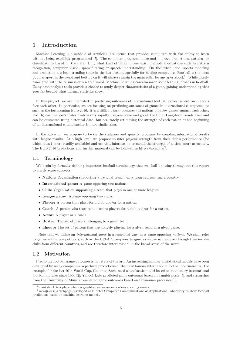
On the other hand, football has become even more interconnected these last years. Figure 1 shows the evolutionsince 1994 of the player club distribution from each World Cup national team3. At the bottom bar, we have thecountries where players come from (clubs) and, at the top, the national teams. Over the years, more playershave gone to play abroad and more football scouts have been interested in foreign leagues.

Figure 1: Evolution of player club distribution from each World Cup national team.

International competitions, such as the Euro, are difficult to predict since national teams play few officialgames and the roasts are volatile from year to year. Nevertheless, we indirectly have a lot of information aboutthe team through their players’ performance in club. Such a joint club/national team model is new and couldpotentially lead to interesting results.

We think there is a new direction in predicting international games where each national team’s fitness isinferred not only for its historical and short-term results but also from the players’ performance in their clubs.To do this, a probabilistic model of pairwise comparison is implemented based on the Bradley-Terry model.

2 Description of the Model

2.1 Bradley-Terry ModelIn this section, we define a theoretical description of our model. From now on, let us consider that a footballgame implicate two teams and results in one of the two teams winning. This assumption is a simplicity of the

3Source: http://www.estadao.com.br/

6

reality, where ties can also appear. We define the probability of the event “team u wins against team v in gamei” as:

p(u � v|i) = 1

1 + exp(−(si,u − si,v)),

where si,u ∈ R is modeled as a linear function and measures the strength of team u at game i.

Notice the similarity with the logistic regression model by just considering si = si,u − si,v as a single variable.This probabilistic model of pairwise comparisons is known as the Bradley-Terry model (BTL) [8]. The BTLscale diference si,u − si,v is a logistic random variable, and so p(u � v|i) can be calculated from the logisticcumulative distribution, as you will see in Section 3. Intuitively, the larger the difference si,u − si,v is, the higherthe probability of team u winning is.

The parameterization of the strength of a team is the crucial part of the model and can be done in a varietyof ways. This variable can depend on the specific game i through well-defined factors such as the lineup of theteam, the location of the game (home advantage) or the historical results between the teams; or other moreindirect antecedents such as the game importance (World Cup final or a friendly), the weather or the playersmotivation. We model the linear function si,u as:

si,u = βTxi,u,

where:

• β ∈ RD is a vector of parameters, and contains the contribution of the total strength of each feature’scoefficient in xi,u.

• xi,u ∈ RD contains the features of team u at game i.

The goal of the inference process is, given xi,u by the data, derive the parameters β. In the followingsubsections we will first introduce the Elo Rating Model, a well-known football ranking system inspired on theBTL model, and later define our own new models.

2.2 Football Elo Rating systemThe World Football Elo Rating system is a football ranking for national teams adapted by Bob Runyan in 1997and publicly maintained in the website elorating.net. This system is originally based on the Elo Rating systemon chess, method for calculating the relative skill levels between players. It is also used in many multiplayercompetitions such as basketball, baseball or videogames [9].

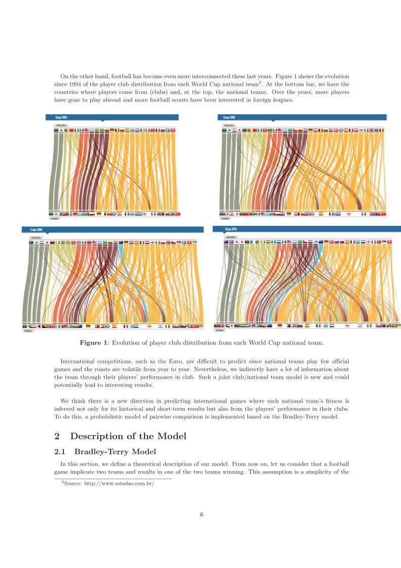
The Elo rating system, like the FIFA system4, is point-based and gives to each match some punctuationdepending on its importance and result. As an example, Figure 2 shows the Elo rating ranking for the nextEuro 2016. However, the main difference between the FIFA ranking is that points are swapped from one teamto another based on: the relative rankings, the goal difference and the ‘win expectancy‘, a predictive measure ofeach team’s likelihood of victory. For each team, a new rating Rn is modified from an old rating Ro based onthe following formula:

Rn = Ro +KG · (W −We)

where:

• K is a constant that measures the importance of the tournament played:

– 60 for World Cup finals.

– 50 for continental championship finals and major intercontinental tournaments.

– 40 for World Cup and continental qualifiers and major tournaments.

4The Fifa World Ranking is an official football ranking for FIFA-recognised national teams based on their game resultswith the most successful teams being ranked highest. http://www.fifa.com/fifa-world-ranking/

7

– 30 for all other tournaments.

– 20 for friendly matches.

• G is the goal difference in the game:

– 1 if the game is a draw or is win by one goal.

– 3/2 if the game is won by two goals.

– 11+N8if the game is won by three or more goals, where N is the goal difference.

• W is the result of the game:

– 1 for a win.

– 0.5 for a draw.

– 0 for a loss.

• We is the expected result (‘win expectancy‘):

–1

1 + 10(−dr/400), where dr equals the difference in ratings plus 100 points for home advantage.

From this last variable, we see that the Elo equation uses a logistic regression model in a similar way thatthe Bradley-Terry model does.

Figure 2: Eurocup 2016 Elo ratings as of Sunday June 5 2016

2.3 Model 0: Team ModelFirst of all, let us define a simple model based on the game outcomes of the national teams. Let NG be thenumber of games and NT the total number of teams. In this model, the goal is to infer the vector of parametersα from the feature matrix S = (si,u) ∈ R

NG×NT , where each row is a game i and each column is a team u.Concretely, we use one parameter for each team, and stack all the parameters into the vector α ∈ RNT . Thefeature vector is given by the indicator vector tu ∈ {0, 1}NT , which is 0 everywhere except at index u where itis 1. Analytically, the strength of team u at game i is defined as:

si,u = αT tu = αu

Hence, we define the vector strength si of the game i (a row of the matrix S) as:

si =

{si,u − si,v if u winssi,v − si,u if v wins

8

In this naive model, the strength of a team is (a) the same for all games, and (b) a priori independent of theother teams’ strength. Notice that as long as clubs do not play against nations, there is nothing that relates clubleagues results with international results. Thus, in international tournaments, the only useful information is theprovided by games where the national teams appear. In summary, incorporating league results in this modelcannot improve our estimation of nations’ strength. This model is essentially the same as the previously definedWorld Football Elo Ratings.

Describing this simple model has two main advantages; on the one hand, it is easy to implement and providesa nice way to get started with inference algorithms, and, on the other hand, it will be a solid baseline againstwhich to compare more complex models.

2.4 Model 1: Actors ModelThe main purpose of this project is the current definition of the Model 1. The team strength si,u of team u

at game i is now modeled as the sum of the player’s performance in their clubs. Informally, we assume that thestrength of a team is defined by the performance of its players on the field.

Let NG be the number of games and NP be the total number of distinct players. As in Model 0, the goal is toinfer the vector of parameters γ from the feature matrix S = (si,p) ∈ R

NG×NP , where each row is a game i buteach column is a player p. Precisely, we use one parameter for each player and we stack them in the parametervector γ ∈ RNP . The feature vector is given by the indicator vector ri,p ∈ [0, 1]NP . In this case, the indicatorvector rather than a binary vector is a vector composed of real numbers between 0 and 1. Each ri,p representsthe ratio of time played by p at the game i (e.g. 1 if p played all the game or 0.5 if half of the game). Analytically,the strength of team u at game i is defined as:

si,u =∑p∈Z

γpri,p

Hence, we define the vector strength si of the game i (a row of the matrix S) as:

si =

{si,u − si,v if u winssi,v − si,u if v wins

The key point of this model is that features are shared across league and international results. Since theinternational games are a small training dataset, we can take advantage of the player’s strengths transfered fromthe national competitions to nations, which are more. To have an idea, our current database stores competitionsfrom a period of 10 years, and there are around 5,000 international games and 30,000 club games.

However, the Actors model might suffer from some drawbacks:

• NP is potentially very large and besides NP >> NG.

• Large fraction of players appear in just few lineups.We can actually solve these two problems if we take a Bayesian inference approach: using the kernel trick,it is not necessary to learn the parameters directly and we can play between the weight space view andthe function space view depending on what we are interested in (infer γ or predict game outcomes).

• The whole might be more that the sum of its parts. A team could be stronger or weaker than simply thesum of its players. There can exists another factors such as the passion to play with the national team orthe feeling between the players that can improve (or worsen) the performance.

2.5 Home advantageOne important parameter that can be additionally included in our model is the home advantage phenomenon.The term home advantage describes the benefit that the home team is said to gain over the visiting team. Thisbenefit has been possibly attributed to supporting crowd effects, travel and changing time zones or climates, oreven referee bias [4]. Maybe the precise causes and the way in which they affect performance are still not clear,

9

but in our constructed database the 57% of victories are from the home teams, and it is a feature that must beconsidered.

Let NG be the number of games and N the length of the vector of parameters β = β0 + β1 + ...+ βN , wherethe first position β0 of the vector is the home advantage feature and the rest of the N − 1 positions are defineddepending on the selected model (for instance, in Model 0 would be the team strengths). The goal is to infer βfrom the feature matrix S = (si,n) ∈ R

NG×N , where each row is a game i and each column n is a feature of β.In the following, it is explained how this first position of β is determined. Analytically, the strength of team u

at game i is defined is:

si,u = βT0 hu + βT

1 xu,1 + ...+ βTNxu,N

where hu is 1 if u wins game i and the game is not neutral5, 0 otherwise. Hence, we define the vector strengthsi of the game i (a row of the matrix S) as:

si =

{si,u − si,v if u winssi,v − si,u if v wins

Then, the first component of the Home advantage model would be:

• 1 if the home team wins and the game is not neutral.• -1 if the away team wins and the game is not neutral.• 0 if the game is on neutral ground.

2.6 Taking advantage of tiesThe first approach was to discard games outcomes that resulted in a tie. Glickman proposed counting ties asone-half of a win, and one-half of a loss [1]. Intuitively, this means that a tie favors small differences in teamstrengths. The “likelihood” of one-half of a win is:

√1

1 + exp(−(βTxi))

Nonetheless, the expectation propagation algorithm cannot deal efficiently with this expression, then it can beapproximated with:

1

1 + exp(−(βTxi)/2)=

1

1 + exp(−(βT xi))

where xi = xi/2. In summary, for every tied game i, we divide it into two data points, xi/2 and −xi/2, and noextra changes are needed in the above-defined models.

2.7 Odds ModelFootball prediction research (and other sports in general) has been carried out by betting companies in thelast 20 years. A well-known example is bwin, one of the world’s largest online gaming businesses, where in 2014their users bet almost 4.000 million of euros and the earnings of the company was 260 million of euros. The keyin the business is to predict the initial odd correctly, and then fluctuate it depending on the volume of the bets.We would ideally like to compare our models against the betting companies predictions and see how close weare, or even if we can get to improve the odds, since they have spent years of investigation in this topic.

5A neutral game is a match where none of the teams played at home.

10

2.7.1 Terminology

In the gambling and statistics context, the odds of some event reflect the likelihood that the event will takeplace. Odds for different outcomes in single bet are presented either in European format (decimal odds), UKformat (fractional odds), or American format (moneyline odds). We have gathered the odds in the Europeanformat from betexplorer.com6 since they represent the inverse of the outcome probability. For instance, if a teamhas an European odd of 2.0, that means it has 1/2 chance of winning. However, an odd of 10 represents a lowprobability (1/10 of winning), and hence more profit if the event occurs.

There exist several types of odds depending on the competition and sport. In relation to the project, we areinterested in two popular football odd types:

• 1x2 betting: also known as three-way betting, and simply refers to betting on a home win, a draw or anaway win.

• Draw No Bet: the draw is eliminated from this bet: it can be only chosen home win or away win. If thegame in question ends without a winner, the money will be returned.

2.7.2 Model

Recall from the definition of the Bradley-Terry model, we still assume binary outcomes, and ties are notconsidered. Similarly, the Odds model defined below is based on Draw No Bet odds, previously removed theoverround7. Moreover, the odds are based on the average of several betting companies, such as bet365, bwin,William Hill or 888sport.

We define the probability of team u wins against team v in game i as:

p(u � v|i) = 1

dnbi,u

where dnbi,u is the Draw No Bet average odd of team u at game i.

3 Model inference

3.1 Bradley-Terry is equivalent to Logistic RegressionIn the Bradley Terry Model, football outcomes are observed as pairwise comparisons. The set of features ofwinning and losing teams of the NG games are collected in a set D = {(xi,w,xi,l)| i = 1, ..., NG}, where w and ldenote the winning and losing team of the game i, respectively. For a given parameter vector β, the model leadsto the likelihood:

p(D|β) =NG∏i=1

1

1 + exp(−(βTxi,w − βTxi,l))

=

NG∏i=1

1

1 + exp(−βTxi)

where we define xi = xi,w − xi,l. Hence, the two models are equivalent since the likelihood is the same asthat of a logistic regression model trained on the binary classification data D′ = {(xi, 1)|i = 1, ..., NG}.6Soccer webpage which offers soccer results, tables, odds stats service for 100+ soccer leagues.7The overround is the percentage of profit that a sportsbook operator has remove from the actual odd value. The lower

the overround percentage, the fairer the market is.

11

3.2 Bayesian InferenceThe first idea to learn the parameters β is to adapt an optimization approach: maximize the likelihood of themodel and perform parameter estimation. There exists multitude machine learning methods to achieve this task.Nevertheless, there are two main backwards:

• Since D is large compared to NG, the estimation would overfit the data and will lead to a poor generaliza-tion. We can solve this problem involving delicately a model fitting function and some sort of regularizationand cross-validation for generalization.

• We cannot deal with uncertainty: we would like to know how confident we are about the predictions.Ideally, we would focus on probabilistic classification, where test predictions take the form of class proba-bilities, in contrasts with binary classification methods which prive only a guess at the class label.

In order to handle these two problems, we will treat β as a random variable. Concretely, we will give a Gaussianprior distribution which with a Bayesian logistic regression would be a particular instance of Gaussian processclassification.

Definition (Weight space view) Given a prior distribution over the parameters, e.g. β ∼ N (0,∑

), findthe posterior distribution (Bayes rule):

p(β|D) ∝ p(D|β × p(β))

With this proposal, we can make assumptions about the characteristics of the underlying functions beforeseeing any data. First, we can restrict the class of functions that we consider, for instance just considering linearfunctions. Second, given a prior probability, we can give higher probabilities to function that we consider morelikely to be. These properties are induced by the covariance function of the Gaussian process.

Since the Gaussian process is not a parametric model, we do not have to worry about whether it is possible forthe non-parametric model to fit the data. Gaussian process for classification links a sophisticated and consistentview with computational tractability. Now, the problem of learning β is transferred to the problem of findingsuitable properties for the covariance function. Furthermore, we actually don’t need to perform inference overβ, but instead only compute the posterior predictive distribution of fi = βTxi.

Definition (Function space view)

p(f |D) ∝ p(D|f × p(f))

That means, the predicted probabilities can be calculated without explicitly infer the vector of parametersβ, dealing with the problem of large D. Moreover, since the posterior update does not have any closed formsolution, we will apply the expectation propagation algorithm, which efficient approximate the inference, usinga public Gaussian processes framework from the University of Sheffield: GPy8.

4 Data collection

4.1 Database structureTo feed and train these models, we need to collect data about the results and participants of national teamsand clubs in the last years. Specifically, we have gathered information from the last 10 years of the followingcompetitions:

• International competitions8GPy is a Gaussian Process (GP) framework written in Python, from the Sheffield machine learning group.

https://sheffieldml.github.io/GPy/

12

Competition Number of gamesUEFA Euro 98

UEFA Euro Qualification 822Confederations Cup 48Friendlies 3903

World Cup Qualification Europe 5365407

Table 1: International competitions where European teams appear

• National leagues

Competition Number of gamesUEFA Champions League 2338UEFA Europa League 4751Premier League 4180Bundesliga 3365

Primera Divison 4175Ligue 1 4178Serie A 4179

27,166

Table 2: Major European leagues and competitions.

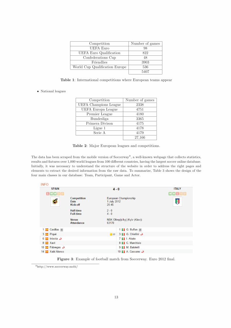
The data has been scraped from the mobile version of Soccerway9, a well-known webpage that collects statistics,results and fixtures over 1,000 world leagues from 100 different countries, having the largest soccer online database.Initially, it was necessary to understand the structure of the website in order to address the right pages andelements to extract the desired information from the raw data. To summarize, Table 3 shows the design of thefour main classes in our database: Team, Participant, Game and Actor.

Figure 3: Example of football match from Soccerway. Euro 2012 final.

9http://www.soccerway.mobi/

13

TeamId

Soccerway IdNameCountry

Alternative names

ParticipantId Is coachGame Is starterTeam Ratio

Actor

GameId Score home

Soccerway Id Score awayTeam home Score home half timeTeam away Score away half timeCompetition Score home full timePhase Score away full timeVenue Score home extra time

Attendance Score away extra timeKickoff time Is neutral

ActorId Nationality

Soccerway Id BirthdayDisplay name PositionFirst name HeightLast name Weight

Alternative names Foot

Table 3: Database tables and fields

After collecting information from 10 different seasons (from 2006 until 2016), there are 924 teams, 39,471 actors,32,229 games and 1,059,387 participants.

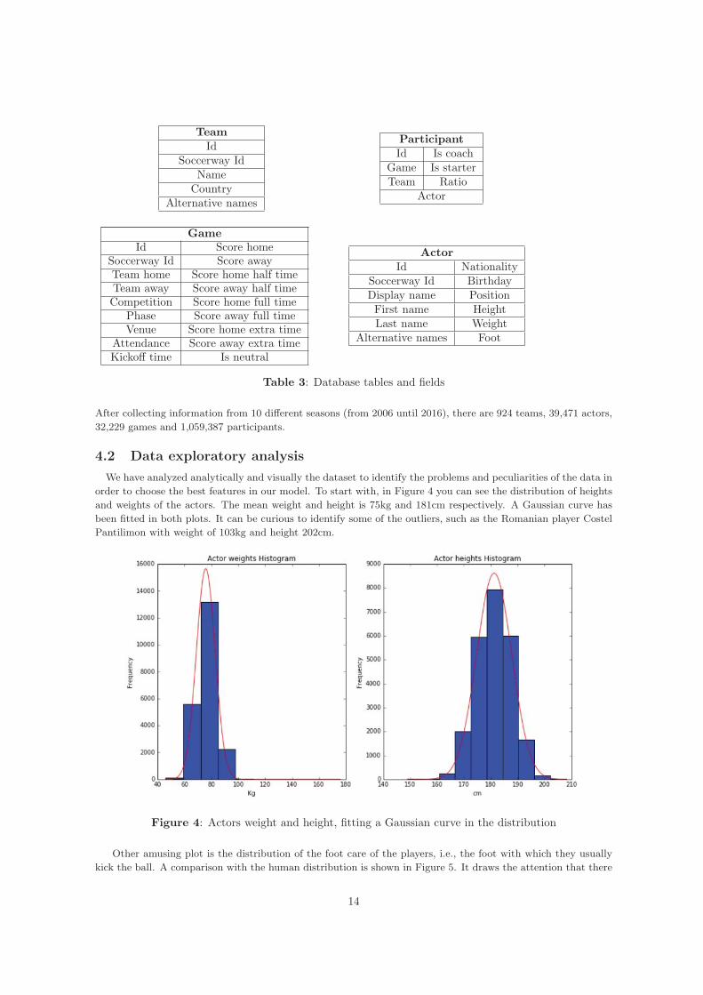
4.2 Data exploratory analysisWe have analyzed analytically and visually the dataset to identify the problems and peculiarities of the data inorder to choose the best features in our model. To start with, in Figure 4 you can see the distribution of heightsand weights of the actors. The mean weight and height is 75kg and 181cm respectively. A Gaussian curve hasbeen fitted in both plots. It can be curious to identify some of the outliers, such as the Romanian player CostelPantilimon with weight of 103kg and height 202cm.

Figure 4: Actors weight and height, fitting a Gaussian curve in the distribution

Other amusing plot is the distribution of the foot care of the players, i.e., the foot with which they usuallykick the ball. A comparison with the human distribution is shown in Figure 5. It draws the attention that there

14

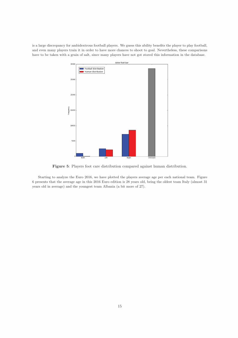
is a large discrepancy for ambidextrous football players. We guess this ability benefits the player to play football,and even many players train it in order to have more chances to shoot to goal. Nevertheless, these comparisonshave to be taken with a grain of salt, since many players have not got stored this information in the database.

Figure 5: Players foot care distribution compared against human distribution.

Starting to analyze the Euro 2016, we have plotted the players average age per each national team. Figure6 presents that the average age in this 2016 Euro edition is 28 years old, being the oldest team Italy (almost 31years old in average) and the youngest team Albania (a bit more of 27).

15

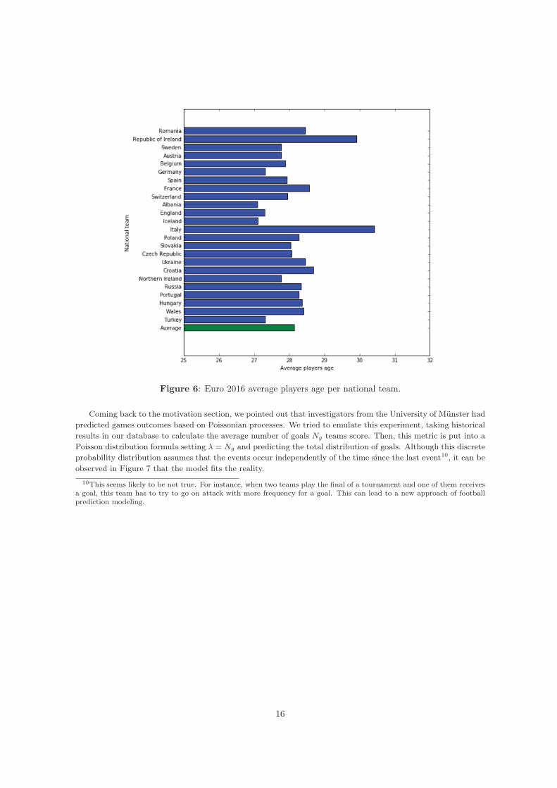
Figure 6: Euro 2016 average players age per national team.

Coming back to the motivation section, we pointed out that investigators from the University of Munster hadpredicted games outcomes based on Poissonian processes. We tried to emulate this experiment, taking historicalresults in our database to calculate the average number of goals Ng teams score. Then, this metric is put into aPoisson distribution formula setting λ = Ng and predicting the total distribution of goals. Although this discreteprobability distribution assumes that the events occur independently of the time since the last event10, it can beobserved in Figure 7 that the model fits the reality.

10This seems likely to be not true. For instance, when two teams play the final of a tournament and one of them receivesa goal, this team has to try to go on attack with more frequency for a goal. This can lead to a new approach of footballprediction modeling.

16

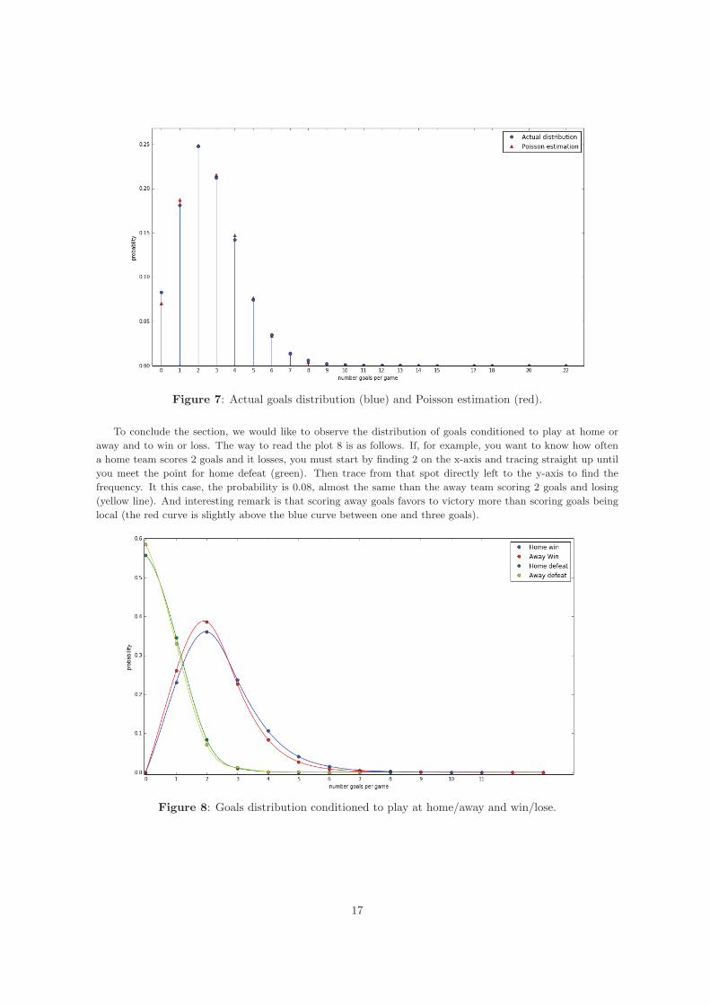
Figure 7: Actual goals distribution (blue) and Poisson estimation (red).

To conclude the section, we would like to observe the distribution of goals conditioned to play at home oraway and to win or loss. The way to read the plot 8 is as follows. If, for example, you want to know how oftena home team scores 2 goals and it losses, you must start by finding 2 on the x-axis and tracing straight up untilyou meet the point for home defeat (green). Then trace from that spot directly left to the y-axis to find thefrequency. It this case, the probability is 0.08, almost the same than the away team scoring 2 goals and losing(yellow line). And interesting remark is that scoring away goals favors to victory more than scoring goals beinglocal (the red curve is slightly above the blue curve between one and three goals).

Figure 8: Goals distribution conditioned to play at home/away and win/lose.

17

5 ResultsIn order to estimate how well the models have been trained and how well they will predict unseen data, thelast Euro editions (2008 and 2012) as well as the Eurocup qualification games (EC Q.) and the World Cupqualification games (WC Q.) from Europe have been used as test sets.

In the following section, the models will be evaluated and compared against the Odds Model using two differentmetrics: 0-1 loss and the log loss. We will explain what results we obtain and the reasons of their behaviors.We will point out what are the weak points of the Actors model and which steps can be taken to improveits performance. Finally, we will conclude the report answering the title of the project: who will be the nextEuropean champion?

5.1 MetricsIn Machine Learning and statistics, different ways of measuring the model performances in terms of metricsare commonly used. In a binary classification scenario, where the target variable has only two possible outcomes,the most well-known metric is the 0-1 loss. Since our classifier uses probabilistic prediction, we have to adaptthe metric to measure the proper accuracy. In this case, just predict the class that has the highest probabilityand compare against the true class.

Definition (0-1 loss) Given the probability pi of the game i:

L0−1 =∑i

yi1{pi≤0.5} + (1− yi)1{pi>0.5}

However, in football prediction we are more interested in measure the uncertainty of the predictions: howconfident we are about them. The log loss measures the uncertainty of the probabilities of a model by comparingthem to the true labels.

Definition (Log-loss) Given the probability pi of the game i:

Llog =∑i

−yi log(pi)− (1− yi) log(1− pi).

The log-loss metric provides extreme punishments for any deviation of the estimate from the data, that is, forbeing both confident and wrong. We will specially interested in this metric to compare the models.

5.2 Home advantage modelWe stated in Section 2 that the home advantage approach would benefit the model performance. Let us checkit empirically. We have used a kernel which is composed of the sum of two different kernels: one for the homeadvantage feature β0 and other for the rest of the vector of parameters. The key here is that when the parametersare optimized, the variance of both parts will be learned independently.

Model 0 log loss 08 Euro 10 WC Q. 12 Euro Q. 12 Euro 14 WC Q. 16 Euro Q.Without home advantage 17.091 100.071 88.487 15.533 90.671 103.699With home advantage 16.949 97.123 85.593 15.506 90.239 103.472

Table 4: Model 0 with and without home advantage comparison.

Model 1 log loss 08 Euro 10 WC Q. 12 Euro Q. 12 Euro 14 WC Q. 16 Euro Q.Without home advantage 17.705 101.716 94.665 14.875 101.400 113.9With home advantage 17.607 100.948 94.095 14.584 100.408 110.601

Table 5: Model 1 with and without home advantage comparison.

Evidently, the performance of both model have improved when the home advantage phenomenon is considered.

18

5.3 Model evaluationAfter the optimization of the parameter variances and compare the performance of different values, we usedin the final evaluation of the models the following hyperparameters:

Model 0Team variance 0.45

Home adv. variance 0.15

Table 6: Model 0 finest parameters

Model 1Player variance 0.035Home adv. variance 0.12

Table 7: Model 1 finest parameters

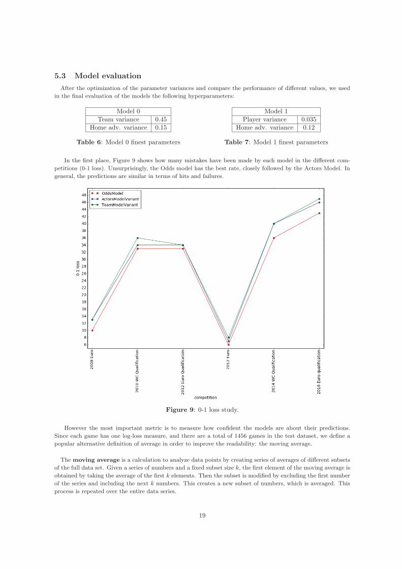
In the first place, Figure 9 shows how many mistakes have been made by each model in the different com-petitions (0-1 loss). Unsurprisingly, the Odds model has the best rate, closely followed by the Actors Model. Ingeneral, the predictions are similar in terms of hits and failures.

Figure 9: 0-1 loss study.

However the most important metric is to measure how confident the models are about their predictions.Since each game has one log-loss measure, and there are a total of 1456 games in the test dataset, we define apopular alternative definition of average in order to improve the readability: the moving average.

The moving average is a calculation to analyze data points by creating series of averages of different subsetsof the full data set. Given a series of numbers and a fixed subset size k, the first element of the moving average isobtained by taking the average of the first k elements. Then the subset is modified by excluding the first numberof the series and including the next k numbers. This creates a new subset of numbers, which is averaged. Thisprocess is repeated over the entire data series.

19

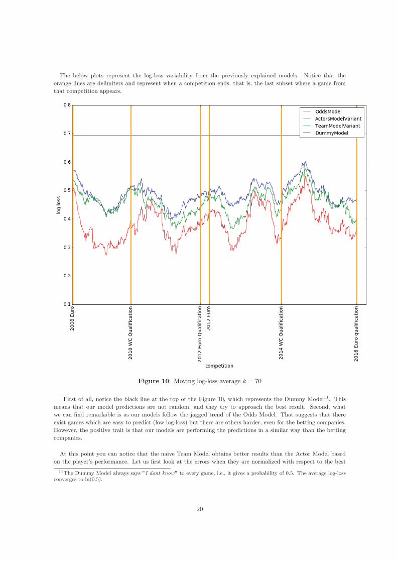
The below plots represent the log-loss variability from the previously explained models. Notice that theorange lines are delimiters and represent when a competition ends, that is, the last subset where a game fromthat competition appears.

Figure 10: Moving log-loss average k = 70

First of all, notice the black line at the top of the Figure 10, which represents the Dummy Model11. Thismeans that our model predictions are not random, and they try to approach the best result. Second, whatwe can find remarkable is as our models follow the jagged trend of the Odds Model. That suggests that thereexist games which are easy to predict (low log-loss) but there are others harder, even for the betting companies.However, the positive trait is that our models are performing the predictions in a similar way than the bettingcompanies.

At this point you can notice that the naive Team Model obtains better results than the Actor Model basedon the player’s performance. Let us first look at the errors when they are normalized with respect to the best

11The Dummy Model always says ”I dont know” to every game, i.e., it gives a probability of 0.5. The average log-lossconverges to ln(0.5).

20

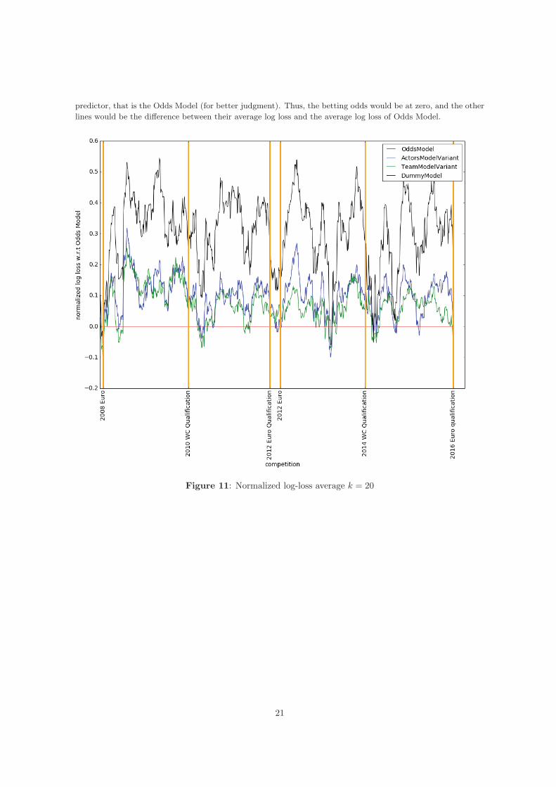
predictor, that is the Odds Model (for better judgment). Thus, the betting odds would be at zero, and the otherlines would be the difference between their average log loss and the average log loss of Odds Model.

Figure 11: Normalized log-loss average k = 20

21

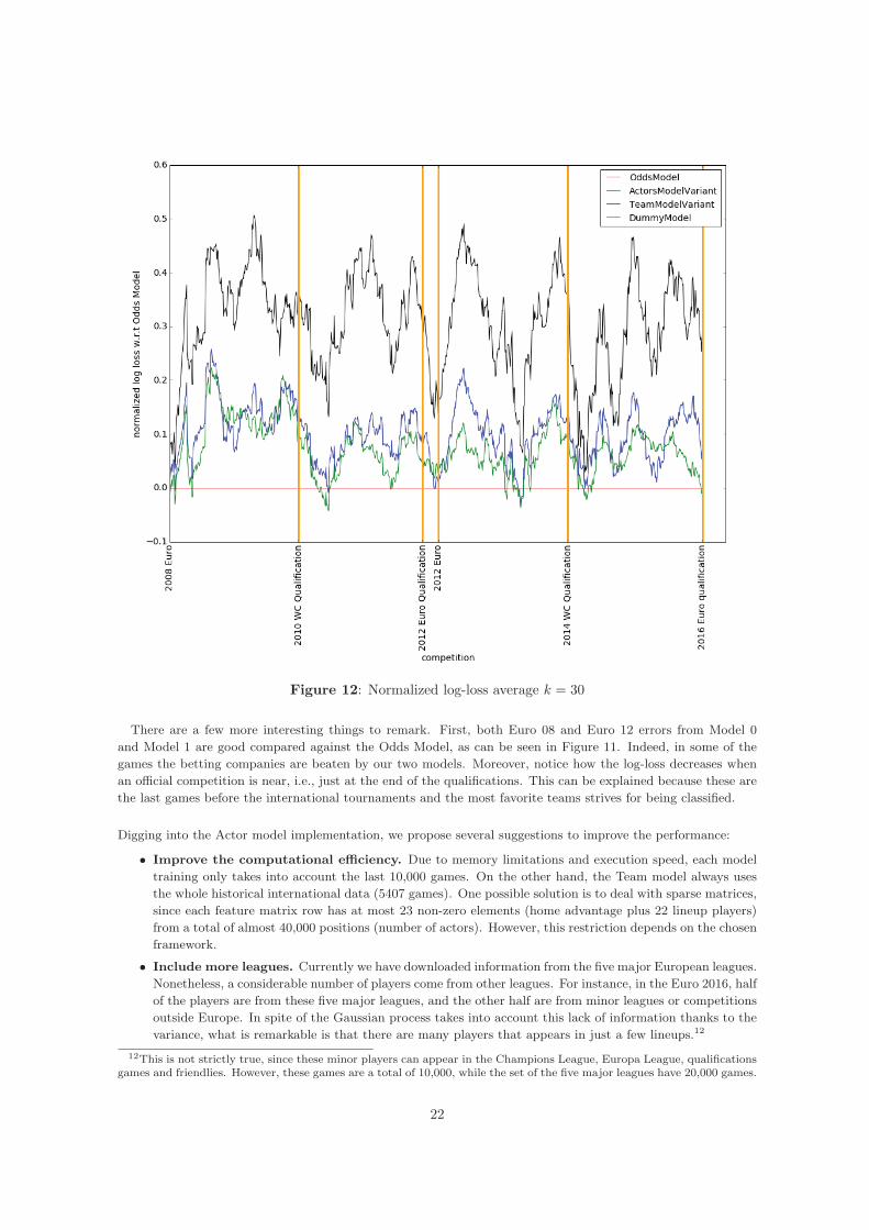
Figure 12: Normalized log-loss average k = 30

There are a few more interesting things to remark. First, both Euro 08 and Euro 12 errors from Model 0and Model 1 are good compared against the Odds Model, as can be seen in Figure 11. Indeed, in some of thegames the betting companies are beaten by our two models. Moreover, notice how the log-loss decreases whenan official competition is near, i.e., just at the end of the qualifications. This can be explained because these arethe last games before the international tournaments and the most favorite teams strives for being classified.

Digging into the Actor model implementation, we propose several suggestions to improve the performance:

• Improve the computational efficiency. Due to memory limitations and execution speed, each modeltraining only takes into account the last 10,000 games. On the other hand, the Team model always usesthe whole historical international data (5407 games). One possible solution is to deal with sparse matrices,since each feature matrix row has at most 23 non-zero elements (home advantage plus 22 lineup players)from a total of almost 40,000 positions (number of actors). However, this restriction depends on the chosenframework.

• Include more leagues. Currently we have downloaded information from the five major European leagues.Nonetheless, a considerable number of players come from other leagues. For instance, in the Euro 2016, halfof the players are from these five major leagues, and the other half are from minor leagues or competitionsoutside Europe. In spite of the Gaussian process takes into account this lack of information thanks to thevariance, what is remarkable is that there are many players that appears in just a few lineups.12

12This is not strictly true, since these minor players can appear in the Champions League, Europa League, qualificationsgames and friendlies. However, these games are a total of 10,000, while the set of the five major leagues have 20,000 games.

22

• Aging factor. Right now, each game is contributing the same weight to the final team strength. Thisdoes not seem entirely reasonable since recent matches are more relevant that games from 10 years agoin order to infer the current performance. We think that implement a continuous decay, where the valueof a game fades exponentially with time, or a step decay, where the value depends on the season, couldimprove the performance of the Actor model.

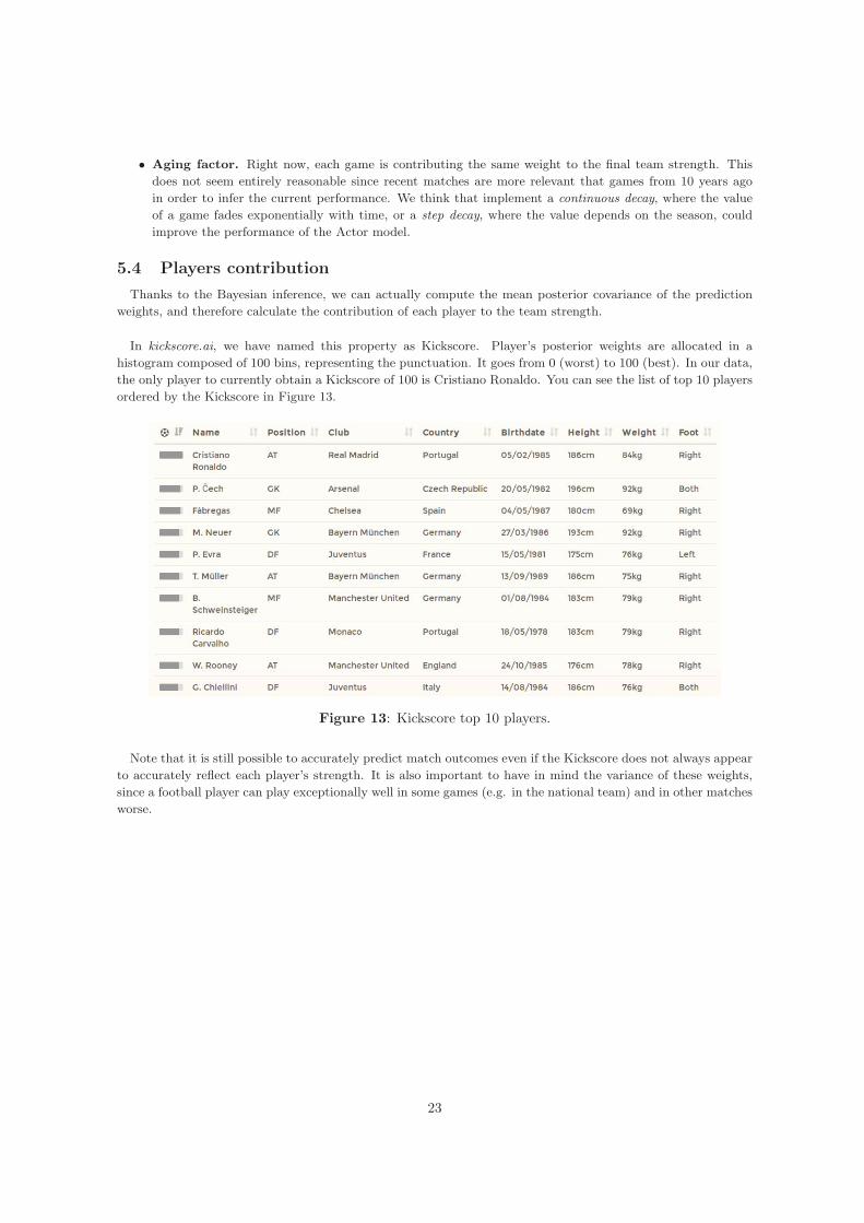
5.4 Players contributionThanks to the Bayesian inference, we can actually compute the mean posterior covariance of the predictionweights, and therefore calculate the contribution of each player to the team strength.

In kickscore.ai, we have named this property as Kickscore. Player’s posterior weights are allocated in ahistogram composed of 100 bins, representing the punctuation. It goes from 0 (worst) to 100 (best). In our data,the only player to currently obtain a Kickscore of 100 is Cristiano Ronaldo. You can see the list of top 10 playersordered by the Kickscore in Figure 13.

Figure 13: Kickscore top 10 players.

Note that it is still possible to accurately predict match outcomes even if the Kickscore does not always appearto accurately reflect each player’s strength. It is also important to have in mind the variance of these weights,since a football player can play exceptionally well in some games (e.g. in the national team) and in other matchesworse.

23

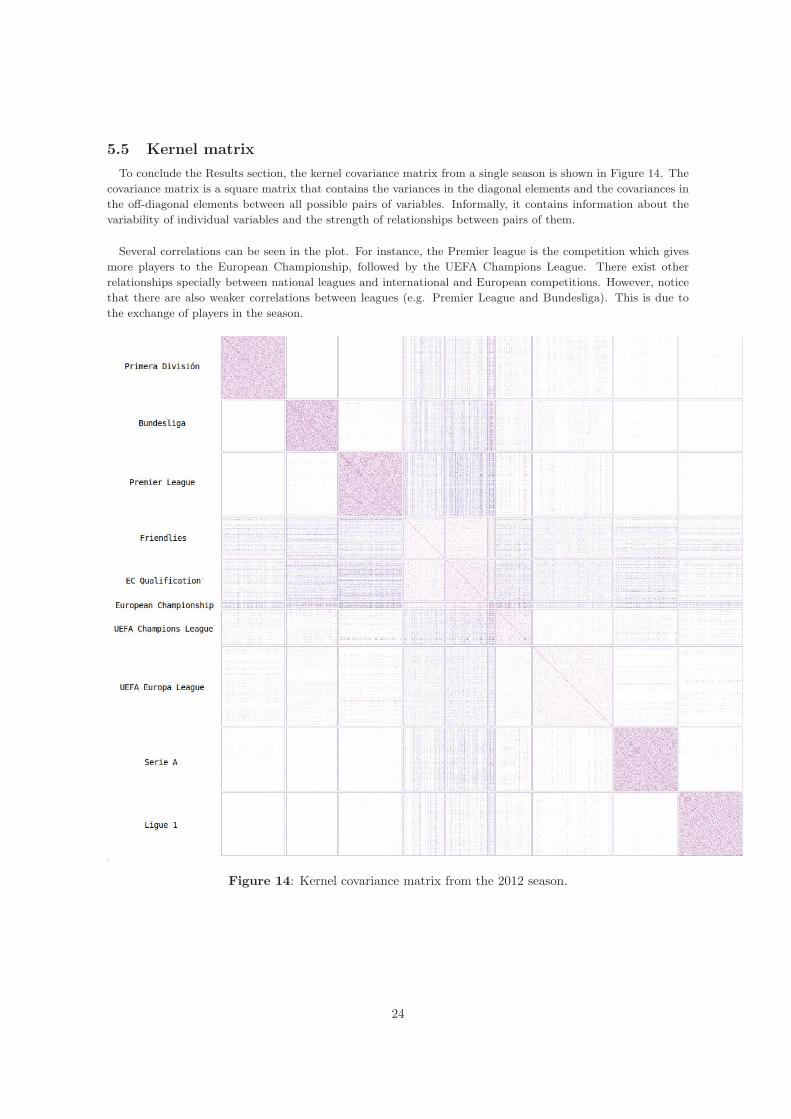
5.5 Kernel matrixTo conclude the Results section, the kernel covariance matrix from a single season is shown in Figure 14. Thecovariance matrix is a square matrix that contains the variances in the diagonal elements and the covariances inthe off-diagonal elements between all possible pairs of variables. Informally, it contains information about thevariability of individual variables and the strength of relationships between pairs of them.

Several correlations can be seen in the plot. For instance, the Premier league is the competition which givesmore players to the European Championship, followed by the UEFA Champions League. There exist otherrelationships specially between national leagues and international and European competitions. However, noticethat there are also weaker correlations between leagues (e.g. Premier League and Bundesliga). This is due tothe exchange of players in the season.

Figure 14: Kernel covariance matrix from the 2012 season.

24

6 Euro 2016 prediction

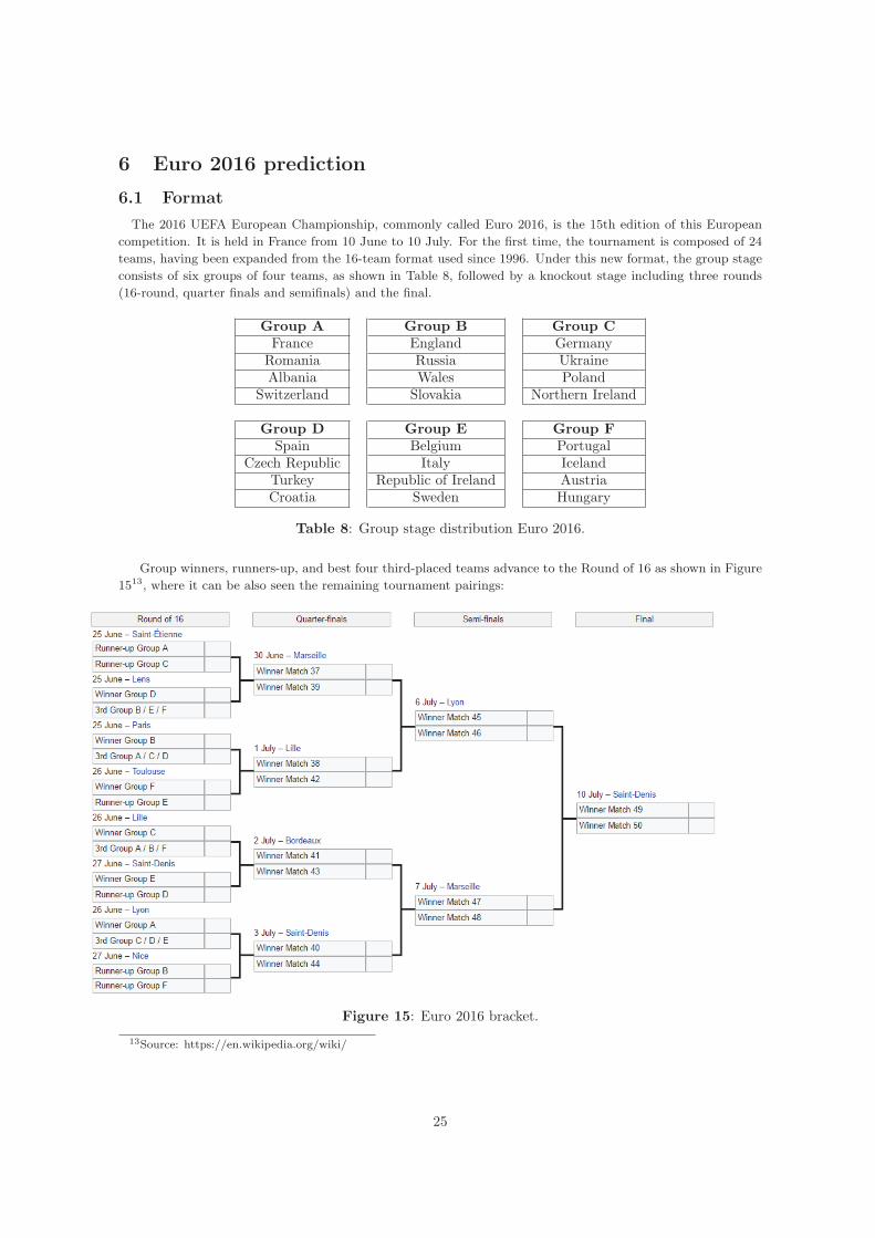
6.1 FormatThe 2016 UEFA European Championship, commonly called Euro 2016, is the 15th edition of this Europeancompetition. It is held in France from 10 June to 10 July. For the first time, the tournament is composed of 24teams, having been expanded from the 16-team format used since 1996. Under this new format, the group stageconsists of six groups of four teams, as shown in Table 8, followed by a knockout stage including three rounds(16-round, quarter finals and semifinals) and the final.

Group A Group B Group CFrance England GermanyRomania Russia UkraineAlbania Wales PolandSwitzerland Slovakia Northern Ireland

Group D Group E Group FSpain Belgium Portugal

Czech Republic Italy IcelandTurkey Republic of Ireland AustriaCroatia Sweden Hungary

Table 8: Group stage distribution Euro 2016.

Group winners, runners-up, and best four third-placed teams advance to the Round of 16 as shown in Figure1513, where it can be also seen the remaining tournament pairings:

Figure 15: Euro 2016 bracket.

13Source: https://en.wikipedia.org/wiki/

25

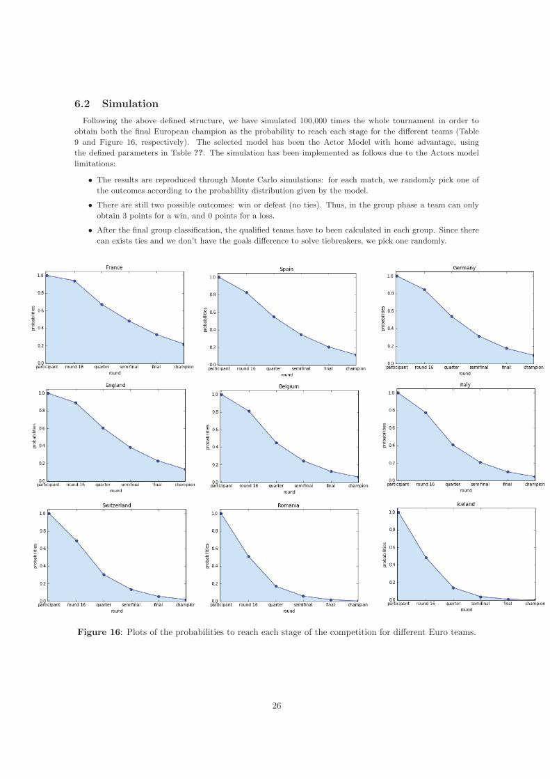
6.2 SimulationFollowing the above defined structure, we have simulated 100,000 times the whole tournament in order toobtain both the final European champion as the probability to reach each stage for the different teams (Table9 and Figure 16, respectively). The selected model has been the Actor Model with home advantage, usingthe defined parameters in Table ??. The simulation has been implemented as follows due to the Actors modellimitations:

• The results are reproduced through Monte Carlo simulations: for each match, we randomly pick one ofthe outcomes according to the probability distribution given by the model.

• There are still two possible outcomes: win or defeat (no ties). Thus, in the group phase a team can onlyobtain 3 points for a win, and 0 points for a loss.

• After the final group classification, the qualified teams have to been calculated in each group. Since therecan exists ties and we don’t have the goals difference to solve tiebreakers, we pick one randomly.

Figure 16: Plots of the probabilities to reach each stage of the competition for different Euro teams.

26

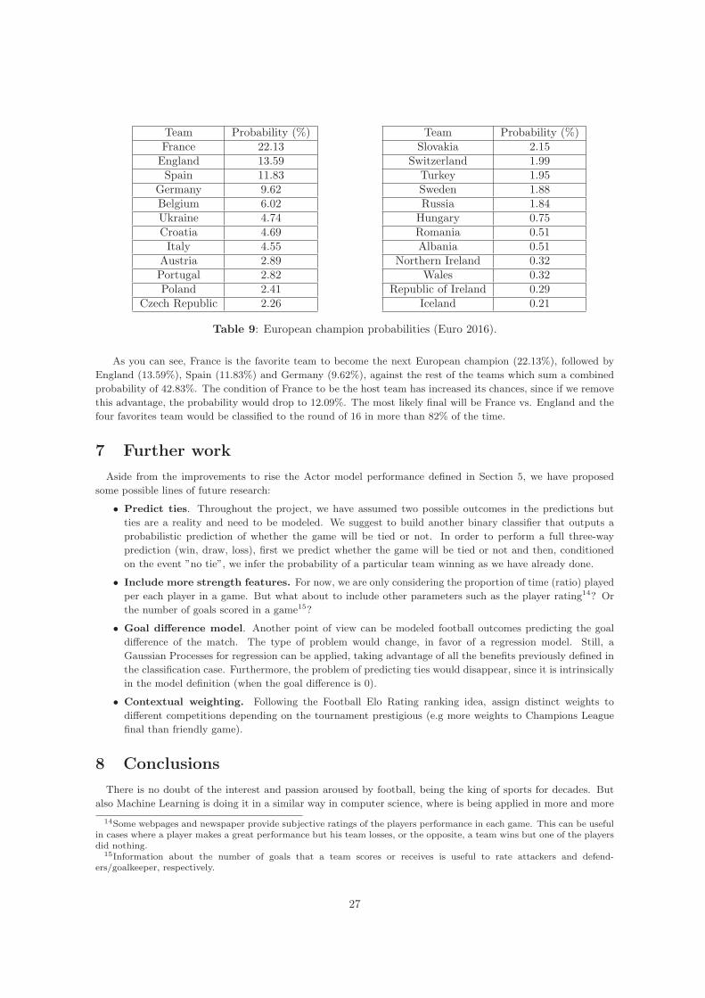
Team Probability (%)France 22.13England 13.59Spain 11.83Germany 9.62Belgium 6.02Ukraine 4.74Croatia 4.69Italy 4.55Austria 2.89Portugal 2.82Poland 2.41

Czech Republic 2.26

Team Probability (%)Slovakia 2.15Switzerland 1.99Turkey 1.95Sweden 1.88Russia 1.84Hungary 0.75Romania 0.51Albania 0.51

Northern Ireland 0.32Wales 0.32

Republic of Ireland 0.29Iceland 0.21

Table 9: European champion probabilities (Euro 2016).

As you can see, France is the favorite team to become the next European champion (22.13%), followed byEngland (13.59%), Spain (11.83%) and Germany (9.62%), against the rest of the teams which sum a combinedprobability of 42.83%. The condition of France to be the host team has increased its chances, since if we removethis advantage, the probability would drop to 12.09%. The most likely final will be France vs. England and thefour favorites team would be classified to the round of 16 in more than 82% of the time.

7 Further workAside from the improvements to rise the Actor model performance defined in Section 5, we have proposedsome possible lines of future research:

• Predict ties. Throughout the project, we have assumed two possible outcomes in the predictions butties are a reality and need to be modeled. We suggest to build another binary classifier that outputs aprobabilistic prediction of whether the game will be tied or not. In order to perform a full three-wayprediction (win, draw, loss), first we predict whether the game will be tied or not and then, conditionedon the event ”no tie”, we infer the probability of a particular team winning as we have already done.

• Include more strength features. For now, we are only considering the proportion of time (ratio) playedper each player in a game. But what about to include other parameters such as the player rating14? Orthe number of goals scored in a game15?

• Goal difference model. Another point of view can be modeled football outcomes predicting the goaldifference of the match. The type of problem would change, in favor of a regression model. Still, aGaussian Processes for regression can be applied, taking advantage of all the benefits previously defined inthe classification case. Furthermore, the problem of predicting ties would disappear, since it is intrinsicallyin the model definition (when the goal difference is 0).

• Contextual weighting. Following the Football Elo Rating ranking idea, assign distinct weights todifferent competitions depending on the tournament prestigious (e.g more weights to Champions Leaguefinal than friendly game).

8 ConclusionsThere is no doubt of the interest and passion aroused by football, being the king of sports for decades. Butalso Machine Learning is doing it in a similar way in computer science, where is being applied in more and more

14Some webpages and newspaper provide subjective ratings of the players performance in each game. This can be usefulin cases where a player makes a great performance but his team losses, or the opposite, a team wins but one of the playersdid nothing.15Information about the number of goals that a team scores or receives is useful to rate attackers and defend-ers/goalkeeper, respectively.

27

areas and many people are interested in learning and research. We have showed that linking these two topicsand taking advantage of the wealth of information available online, surprising results can be reached.

Modeling the team’s strength as the sum of the strength of the players allows to use many parameters that arenot available in just international competitions, enriching the predictions. Promising results have been showncompared to the betting companies, in spite of the simplicity of the model. We think that including more complexparameters, such as the aging factor or the ties prediction would lead to rising results. Moreover, combiningGaussian processes, which concede a huge flexibility and easy intuition in modeling, and pairwise comparisons(e.g. football outcomes) have shown satisfactory experimental outcomes. Thanks to the Bayesian inference, weare able to understand how confident we are about the predictions in order to correctly interpret them.

To conclude, France has the highest probability of being the next Euro champion, but this does not mean itwill happen. Focusing on a particular prediction misses the big picture, which is the overall accuracy when allmatches are taken into account. Football matches are not completely predictable and there exist a countless ofvariables that are impossible to model. Perhaps, this is what makes this sport so fascinating.

AcknowledgmentsI would like to thank Lucas and Victor, with whom I have enjoyed a lot working on the project and they helpedme whenever I needed. Also thanks to the LCA group and Prof. Matthias Grossglauser who have showed methan machine learning can be even more interesting than what I had ever thought.

References[1] Mark E. Glickman; Parameter estimation in large dynamic paired, comparison experiments , Boston Uni-versity, USA, 1999

[2] Jan Hatzius, Sven Jari Stehn and Donnie Millar; A statistical model of the 2014 World Cup, Goldman SachsGlobal Investment Research, 2014.

[3] A. Heuer, C. Muller, O. Rubner; Soccer: Is scoring goals a predictable Poissonian process?, University ofMunster, 2014.

[4] Richard Pollard; Home Advantage in Football: A Current Review of an Unsolved Puzzle, California Poly-technic State University, 2008.

[5] Vladan Radosavljevic, Mihajlo Grbovic, Nemanja Djuric and Narayan Bhamidipati; Large-scale World Cup2014 outcome prediction based on Tumblr posts, Yahoo! Labs, Sunnyvale, USA, 2014.

[6] C. E. Rasmussen and C. K. I. Williams, Gaussian Processes for Machine Learning, MIT Press, 2006

[7] Phil Simon; Too Big to Ignore: The Business Case for Big Data, 2013

[8] Kristi Tsukida and Maya R. Gupta; How to Analyze Paired Comparison Data, University of Washington,2011.

[9] Been Wood; Enemydown uses Elo in its Counterstrike, TWNA Group.

28