Hanson, Kevin. 2010. Development and Assessment of a GIS Based Model to Identify Sand and Gravel Resource Potential to Assist in the Acceleration of Aggregate Resource Mapping by the Minnesota Department of Natural Resources. Volume 12, Papers in Resource Analysis. 25pp. Saint Mary’s University of Minnesota Central Services Press. Winona, MN. Retrieved 12.05.2010 from http://www.gis.smumn.edu

Development and Assessment of a GIS Based Model to Identify Sand and Gravel Resource Potential to Assist in the Acceleration of Aggregate Resource Mapping by the Minnesota Department of Natural Resources Kevin J. Hanson

Department of Resource Analysis, Saint Mary’s University of Minnesota, Winona, MN 55987 Keywords: GIS, Aggregate Resource Potential, Sand and Gravel, MN DNR, Aggregate Resource Mapping, Models, Gravel Pits, Surficial Geology, SSURGO, Raster Analysis Abstract The Minnesota Department of Natural Resources (MNDNR) Aggregate Resource Mapping Program (ARMP) was created in 1984 by the MN Legislature Statute 84.94 to protect construction aggregate resources by identifying and classifying potential sand and gravel deposits or crushed stone resources in Minnesota counties. Since 1984, the mapping of 23 counties’ aggregate resource potential has been completed, four projects are near completion or in-progress, and there are 8 counties requesting mapping. As Minnesota’s population continues to grow there is a significant need to accelerate the mapping of construction aggregate resources to assist in their protection. To address the need, a pilot project was set up to develop a geographic information systems (GIS)-based model that identifies the locations of significant and nonsignificant sand and gravel resources based upon ARMP aggregate mapping classifications. The model developed was tested in Carlton County, Minnesota and the Fond du Lac Reservation. The model applied four 10-meter cell grids derived from the following sources, in order of importance: Minnesota Geological Survey (MGS) Surficial Geology (scale 1:100,000), Soil Survey Geographic (SSURGO) database (1:20,000); MGS maintained County Well Index (CWI) stratigraphy database; and identified sand and gravel pits and prospects. The second objective of the project was to determine the validity of the model’s results by completing a raster comparison analysis with the sand and gravel resource potential from the MNDNR’s ARMP map publication, “Aggregate Resources of Carlton County and Fond du Lac Reservation.” A comparative 10-meter raster analysis was chosen and displayed the final modeled cells equaling 93 percent of the published ARMP map source cells. More specifically, the final model equaled 94 percent of the nonsignificant potential ARMP cells, and 66 percent of the significant potential cells. It is important to note that ARMP’s significant potential map units only equaled 4.5 percent of the total study area while nonsignificant potential equaled 95.5 percent. The GIS model proved to be an effective tool at modeling sand and gravel resource potential. It is best utilized by ARMP geologists as an interpretive tool to map counties more efficiently. Introduction Construction aggregate resources

include sand and gravel and crushed stone. Sand and gravel deposits are rock fragments that have been naturally

2

shaped by the weathering of the bedrock and subsequent transportation and deposition by glaciers (Langer, 1988). In contrast, crushed stone is created by machines that break bedrock into small angular fragments (Langer, Drew and Sachs, 2004). Based on value and volume, aggregate resources are the largest non-fuel industry in the world, exceeding copper and gold by $11.5 billion in 2003 (Langer et al., 2004). Aggregate is produced in all 50 states, and in each of the 87 counties of Minnesota. Each of us in the United States consumes ten tons of aggregate per year (Langer et al., 2004). Sand and gravel resources are high-bulk, low-value commodities. This means one ton of sand and gravel may cost only $5 - $15 dollars at the mine, but when delivery is figured in, the transportation will account for a considerable portion of the delivered price. In fact, the cost of a project approximately doubles for every 20-30 miles the aggregate is transported (Ad Hoc Aggregate Committee, 1998). A city of 100,000 people can expect to pay an additional $1.3 million each year for each ten miles the aggregate it uses has to be hauled (Langer et al., 2004). Figure 1 displays haul trucks being loaded at a sand and gravel pit near Grand Rapids, Minnesota.

Figure 1. Trucks hauling sand and gravel out of a gravel pit site near Grand Rapids, MN.

In Minnesota the population is expected to grow 24 percent between 2005 and 2035 (State of Minnesota Demographics Center, 2007). With the rapid growth of Minnesota, the Twin Cities and other regional centers across the state, cities are expanding into previous rural areas. In these increasingly metropolitan areas, urban growth has led to the covering of some deposits (sterilization) and depletion of other existing aggregate reserves. Often, communities oppose the permitting of new mines (Southwick, Jouseau, Meyer, Mossler and Wahl, 2000). Eng and Costello (1979) highlight this sentiment, “aggregate resource encumbrance, as demonstrated in many urban areas, is the prevailing land use sequence of urban sprawl. No improvement can be expected unless this trend stops or our mineral lands are otherwise protected.”

Tepordei (1999) at the USGS suggests that the total amount of mined construction aggregates in the next 25 years will be equal to the past 100 years of aggregate mined in the United States. Tepordei goes on to write that, “these projections suggest that the vast quantities of crushed stone and sand and gravel will be needed in the future and that much of it will have to come from resources yet to be delineated or defined. Therefore interdisciplinary scientific studies specifically relevant to the aggregates industry will be needed even more in the future.” This fact, in combination with increasing land use conflicts and increasing delivery distance, highlight the importance of inventorying aggregate resources before they are irretrievably lost.

Legislation at the State of Minnesota put forth Minnesota Statute, Section 84.94, 1984, to plan for and protect existing aggregate resources, to

3

spread the impact of development, and to promote orderly and environmentally sound development of the resource. As a direct result, the Aggregate Resource Mapping Program (ARMP) was created. The statute assigns the MNDNR Division of Lands and Minerals in cooperation with the MGS and Minnesota Department of Transportation (MNDOT) to identify and classify potential valuable aggregate-bearing lands at the county level. The counties closest to major urban sectors were given higher priority.

The information and digital data produced by ARMP has evolved since 1984 as GIS technology has advanced and become more accessible. Today, each county completed is given the following information: printed and digital maps of county-wide aggregate resource potential; GIS data of aggregate resource potential, gravel pit and quarry inventory, and field observations; a PowerPoint presentation specific to each county’s aggregate resources; and a public interactive web mapping server of all the GIS data on the MNDNR webpage.

The information, maps, and digital GIS data given to each county is intended to assist county planners and staff in making land management and zoning decisions in regards to aggregate resources.

As seen in Figure 2, 23 counties have been completed, four projects are near completion or in-progress, and eight counties have requested aggregate mapping. Due to the large number of counties requesting mapping and the limited resources available to complete each project, it is beneficial to maximize efficiency in mapping each county. Historically, the length of time it takes to map a county has ranged from one to

five years depending on the size of the county, existing digital data sources, and staff size at ARMP. Current Aggregate Mapping Methods The aggregate mapping methods used by ARMP combine traditional geologic data gathering and mapping (i.e., fieldwork and drilling) with GIS. Sand and gravel resource mapping is accomplished by first gathering and summarizing existing data. The next task is to collect new data points in the field through observation, hand sampling and drilling. The last step is to interpret all data sources and classify the aggregate resource potential in ArcGIS Desktop with lines and points.

Figure 2. Graphic of Minnesota depicting ARMP status as of August 2010.

Before any mapping begins, the geologist must conduct a literature review and digital data search. Digital data compiled includes, but is not limited to; existing surficial geology datasets, SSURGO soils database, current and historical aerial photographs, USGS topographic quadrangle maps,

4

digital elevation models, CWI locations and stratigraphy database, gravel pit and gravel pit prospects data, historic geology maps, wetlands, lakes, streams, vegetation, land use data, and assorted base map data. All data is loaded onto tablet computers with ArcGIS Desktop and used in the field by the project geologist.

Depending on the size of the project area, eight weeks to eight months are spent in the field driving all accessible roads, digitizing points, and entering the attribute data for geologic observations. The geologic observations collected range from a stream exposing sand and gravel to the determination of overburden and thickness of sand and gravel in a gravel pit to drilling a 20-foot deep test hole and analyzing the materials with a sieve in a lab. All of these observations assist in confirming or negating the existence of sand and gravel deposits.

Through the combination of geologic field observation, drilling, and the compiled spatial datasets, the project geologist interprets the geographic distribution of aggregate resources by digitizing lines and points in ArcGIS Desktop. The root of this mapping technique is known as the landsystems approach.

The landsystems approach principle is that glacial landforms, like eskers and end moraines for example, deposited a predictable range of sediments. Sediments include sand and gravel, silts, clays, and other unsorted materials. Several other general characteristics assist in interpreting the surface materials of a landform, like tonal contrasts, texture, context, shape, size, trend, association, and patterns. One example is that vegetation, which grows on well-drained soils like sand

and gravel, will have a unique texture, tone and pattern in aerial photographs. Sand and gravel bearing landforms, like outwash channels, eskers, and terraces can be seen using the above mentioned technique.

Figure 3. Graphic of Carlton County and Fond du Lac Reservation that displays the four classes of sand and gravel resource potential mapped by MN DNR’s ARMP (Friedrich, 2009).

The digitized lines and points are applied topology rules in ArcGIS and then converted to polygons. The points contain the attributes to each polygon, such as sediment type, landform, classifications for sand and gravel potential, probability, deposit size, texture, material quality, thickness, overburden, and glacial lithology. The points are then joined to the polygons using the Spatial Join tool in ArcToolbox. The finished polygons can be used to make maps as seen in Figure 3, Map of Sand and Gravel Resources of Carlton County and Fond du Lac Reservation completed by the MNDNR’s ARMP project geologist Hannah Friedrich (Friedrich, 2009). The map shown in Figure 3 is symbolized using the four sand and gravel potential

5

classes: high potential, moderate potential, low potential, and limited potential. ARMP defines significant aggregate resources as those with high and moderate potential and nonsignificant aggregate resources as those with low and limited potential. Model Development A literature review for this project was unable to find GIS applications developed to determine sand and gravel potential at a reconnaissance level scale of 1:100,000 or 1:50,000. As a result, a pilot project was initiated with support from the MNDNR’s ARMP, to develop a GIS model that maps significant and nonsignificant sand and gravel resource potential by using only existing spatial datasets in the model. Using this model, there would be no field work, drilling, aerial photo interpretation, or digitizing of lines and points.

The project area for the model seen in Figures 4 and 5 included all of Carlton County, Minnesota and the Fond du Lac Reservation, whose northern boundary intersects southern St. Louis County. The model results were assessed for validity by comparing them in a 10-meter cell-to-cell raster analysis to the significant and non-significant sand and gravel resource potential of Carlton County, MN and the Fond du Lac Reservation mapped by MNDNR’s ARMP published in June 2009 (Friedrich, 2009). Overview of Existing Vector Spatial Datasets Used in the Model A total of five grids were developed and applied into the model. These were: MGS Surficial Geology, SSURGO Soils, CWI Verified Well Stratigraphy,

historic and current gravel pits and prospects, and a layer that merged MGS bedrock outcrops and lakes greater than five acres.

To create each grid, existing vector spatial datasets were compiled and reclassified using ArcGIS Desktop with the aid of an ARMP project geologist. This section is a discussion of the vector spatial datasets applied in the model.

Figure 4. Graphic showing the location of the project area relative to the State of Minnesota.

Figure 5. Graphic showing the location of the project area relative to Minnesota County Boundaries. Surficial Geology Vector Data

6

The landsystems approach discussed in this paper assists in identifying the distribution of sand and gravel bearing landforms. These landforms are best displayed on surficial (quaternary, glacial) geology maps. Surficial geology maps delineate glacial landforms such as eskers, end moraines, and outwash channels. No other spatial dataset applied in this model carries more weight in identifying sand and gravel resources than surficial geology. The scale that a surficial geology dataset is mapped plays a vital role in the model’s success. Using too small a scale, such as 1:500,000, would not be appropriate for a reconnaissance level map of 1:100,000 to 1:50,000. The MGS’s County Geologic Atlas Program creates GIS data and maps of surficial geology at the 1:100,000 scale. For this model the MGS’s GIS data of surficial geology of Carlton County, MN and Fond du Lac Reservation (Knaeble and Hobbes, 2009) was applied. Soils Vector Data Soil spatial databases are an existing GIS layer that can identify near surface sediments (within six feet of surface) as well as the parent material of the soils. The parent material in general is the surficial geology.

The two most common soil databases used are the State Soil Geographic (STATSGO) and Soil Survey Geographic (SSURGO). The STATSGO database is intended to be used primarily for regional, state, and multicounty resource planning. According to the United States Department of Agriculture (1995), “STATSGO data are not detailed enough to make interpretations at a county

level.” SSURGO data however are much more detailed than STATSGO data. The USDA (1995) further states that, "SSURGO database provides the most detailed level of information and was designed primarily for farm and ranch, landowner/user, township, county.” In addition the USDA (1995) indicates that, “using the soil attributes, this database serves as an excellent source for identifying sand and gravel aquifer areas.” A map displaying the status of SSURGO mapping in Minnesota is seen in Figure 6.

Figure 6. Graphic of Minnesota depicting SSURGO soils status as of January 2010. Because of its higher level of detail over STATSGO data, the SSURGO geographic soil database of Carlton County and Southern Saint Louis County were chosen for inclusion in this project’s model. This specific database has a scale of 1:20,000 (USDA, 2006). County Well Index Vector and Tabular Data

7

The Minnesota County Well Index (CWI) database is a statewide spatial dataset of approximately 196,000 verified well locations and 208,000 unverified well locations as of June 2010. This database is maintained and updated by the MGS in collaboration with the MN Department of Health (MNDOH). These wells vary in scale due to the methods used to digitize the well location. Some wells were located with a GPS at the well site while others were drawn on a 1:24,000 USGS topographic map and later digitized. Due to the uncertainty of the spatial locations of the unverified wells they were not considered for this project.

Most of the verified well records in CWI contain a primary key field (REALTEID) that can be related as a one-to-many relationship to a separate table of stratigraphic records. The stratigraphy table lists the lithology of the well’s subsurface materials which is primarily determined by the driller of the well. The lithology is a very useful tool for modeling sand and gravel resource potential since it provides a greater view of the subsurface materials. However, significant reclassifications needed to be implemented in the database in order to model the well’s stratigraphic data given the extensive variability in the driller’s description. For example, as seen in Figure 7, there are 3,316 verified wells in the project area. From those wells there are 16,049 stratigraphic records based on the one-to-many relationship. From those 16,049 records there are 1,696 unique material descriptions under the driller description field (DRILL_DESC). Those 1,696 descriptions were reclassified down to 72 unique material descriptions and ranked relative to sand and gravel potential. This reclassification will be

explained in greater detail in the next section.

Figure 7. Graphic of the project area that displays the 3,316 verified CWI wells and number of stratigraphic records included in the model. Identified Sand and Gravel Resources Vector Data The final vector layer of the model consists of points of current and historic gravel pits, sand pits, and potential future sand and gravel prospects. This point dataset is derived from a variety of different sources from the following agencies: MNDOT, USGS, MNDNR, and USDA.

MNDOT’s Aggregate Source Information System (ASIS) is a statewide database that contains the locations of 7,794 gravel pits, sand pits, crushed stone quarries, and prospects. This is the most accurate database of current construction aggregate sources for the state of Minnesota. Within the project area there are 67 sand and gravel pit sources and 191 prospects of varying quality.

The USGS topographic 7.5 minute quadrangle maps display the locations of gravel pits, sand pits,

8

quarries, and taconite mines. The majority of these locations were digitized by the MNDNR in 2004, though the dataset was never officially published. Data gathering stopped before digitizing was completed for the entire state. Moreover, the dataset has never been quality checked. For this project only the USGS data where gravel pits and sand pits were greater than a quarter mile away from an ASIS source was included. There were a total of 104 points merged into the final dataset.

The USDA SSURGO dataset includes a point layer called Spot Feature Points which include various observed features (USDA, 2006). Those relevant to this project include gravel pit, sand pit, sandy spot, or gravelly spot. There are a total of 80 SSURGO sourced gravel pits merged into the final dataset. These 80 points are all located greater than a quarter mile from any other MNDOT or USGS sourced gravel pit to limit redundancy in data sources. Additionally, there were 609 other features (sandy spot, gravelly spot, knoll of better drained soil, etc.) merged into the final dataset.

A total of 1,051 point features make up the final dataset seen in Figure 8. Each of these points was given a sand and gravel potential rank index to be weighted in a kernel density model. The density model and ranks will be discussed in the next section. MGS Bedrock Outcrops and Lakes Vector Data In general, there is no potential for sand and gravel resources where the bedrock is at the surface. Therefore, all bedrock outcrops were used to erase areas of potential in the final grids. It should be noted that certain types of bedrock can

be used for crushed stone aggregate resources, though this project’s scope includes modeling sand and gravel resources only. The bedrock outcrops used for this model are polygons and were derived from MGS’s Geologic Atlas of Carlton County, MN, which does include the Fond du Lac Reservation (Knaeble et al., 2009).

Figure 8. Graphic of the project area that displays gravel pits, sand pits, sand and gravel prospects, and additional aggregate features.

MGS surficial geology maps sometimes map the surficial geology below the lake bed, though most (especially the 30 x 60 minute quadrangle maps) delineate only the water bodies or lakes themselves. The MGS GIS dataset for surficial geology of Carlton County does map below the lake bed, however none of the other datasets used in this model do. The SSURGO soils database is included in those that map only the bodies of water without the underlying surficial geology. ARMP did delineate the landforms under the lake bed for their Carlton County and Fond du Lac Reservation map. However, while the GIS data of MGS and ARMP will at times show the surficial geology mapping units below

9

the lakes, the cartographic printed maps will cover up or erase the surficial geology mapping units with lakes in order to give spatial reference to the map reader. Given this background, it was decided not to attempt to model below the lake bed. Using the ArcGIS Update tool in the Analysis Toolset the MGS surficial geology, SSURGO soils, and ARMP’s sand and gravel resource potential were all updated with a GIS dataset of lakes that are greater than five acres sourced from the MNDNR.

The lakes and bedrock outcrops (Figure 9) were merged together and given a value of 0 within a unique field. The merged layer was then dissolved on the unique field using the ArcGIS Desktop Dissolve tool.

Figure 9. Graphic of the project area that displays MGS bedrock outcrops and lakes that are greater than 5 acres. Limitations in Map Scale The map scales of the vector datasets range from 1:100,000 surficial geology map down to GPS level of detail (+/- 30 meters) on some CWI wells. The scale of each dataset reflects its level of detail or resolution (Tomlinson, 2003). When modeling data sets of different scales

together there is an inherent loss of accuracy. Because of this imprecision, the model should always be interpreted with knowledge of all the map scales from the inputted datasets. Furthermore, the final grid was given a scale of the smallest scale dataset (lowest resolution) used in the model. For this model it would be the MGS surficial geology at 1:100,000. Ranking the Vector Data and Converting to Grid Surficial Geology The MGS surficial geology map units and original map with detailed map unit descriptions were given to ARMP project geologist, Hannah Friedrich, to reclassify with a rank from 0-10. The ranking system was based on the

interpretation of the mapping unit as it relates to potential for sand and gravel resources seen as followed: limited potential 0-2; low potential 3-4; moderate potential 5-7; and high potential 8-10 (Table 1).

The vector data was then converted to a raster grid at 10-meter resolution. Figure 11 in Appendix A displays the surficial geology mapping units as a grid subdivided into four classes. SSURGO Soils The SSURGO geographic map units used in the model were from the parent group material field (pmgroupnam). Another field displayed in combination with the parent group material was the geomorphic description field (geomdesc). These mapping units and a detailed map were again given to ARMP project geologist, Hannah Friedrich, to

10

reclassify with a rank from 0-10 as with the surficial geology (Table 2).

The vector data was then converted to a raster grid at 10-meter resolution. Figure 12 in Appendix A displays the SSURGO mapping units as a grid subdivided into four classes. Table 1. MGS Surficial Geology Map Unit Rank.

Modeling the CWI Stratigraphy Within this pilot model the CWI stratigraphy table dataset required the most intensive analysis and reclassifications. It involved modeling each subsurface record’s material, thickness, and depth from surface and calculating it into a single numeric which would be summed with the other

records within that well log. After this analysis, each well had a single numeric that represented the subsurface material’s thickness and overburden as it related to sand and gravel resources. The number was applied in an inverse distance weighted (IDW) interpolation using the Spatial Analyst extension in ArcGIS Desktop. The resulting grid was clipped in areas where there was no well within one mile of another well. This is known as the data gap. Finally, the resulting grid was reclassified into values between 1 and 10 for inclusion into the final model. Table 2. SSURGO Soils Map Unit Rank.

The first objective was to rank

the subsurface material of each stratigraphic record (Table 3). The records seen in Table 3 were reclassified from 1,696 unique driller descriptions (DRILLR_DESC). Fortunately, for the

11

great majority of these records the MGS had reclassified the driller description field into one, two, or sometimes three additional fields that represented the primary, secondary, and minor lithology. For example, if the driller description was ‘Sand & Gravel’ the primary lithology (LITH_PRIM) field would be sand (‘SAND’) and the secondary lithology (LITH_SEC) would be gravel (‘GRVL’). Note, for this study the primary lithology field contains 38 unique records and the secondary lithology field contains 35 unique records. From those there could be many possible variations. Some examples would include: sand and gravel, sand and clay, gravel and clay, gravel and sand and so on.

To simplify these overlapping designations, a new field was added to reclassify the three fields into one field. The new field’s (STRAT_MAT) attributes are shown in Table 3. The resulting unique material descriptions were given to ARMP project geologist, Hannah Friedrich, to rank according to aggregate potential. Further reclassification was needed on certain ranks in order to minimize calculations on the nonsignificant sand and gravel materials that may have deep wells. For example, materials with primary clays, silts, and sands, or those same materials with some gravel, were initially given a rank between 0 and 5. The majority of these were reclassified to values between 0 and 2 to limit their presence in the final grid. The final rank of the stratigraphic material is seen in Table 3 under ‘Model Rank Index’.

The thickness of each material was determined by subtracting the depth to top field (DEPTH_TOP) from the depth to bottom (DEPTH_BOT) field in the stratigraphy table.

Table 3. CWI Index Stratigraphy Material Rank (SMR).

Thickness of Stratigraphic Material (TSM)

= (DEPTH_BOT – DEPTH_TOP)

The overburden of the material,

otherwise explained as “depth below surface” determines the viability of extracting a material. In general, the more overburden the less likely the sand and gravel resource will be extracted. The overburden value can be found in

12

the CWI stratigraphy table under the depth to top field (DEPTH_TOP).

Overburden of Stratigraphic Material (OSM)

= DEPTH_TOP

The overburden fields were

reclassified into five numeric classes based on a range of overburden of values in feet as seen below:

0–15 feet = 1.0 16-30 feet = 0.75 31-50 feet = 0.50 51-100 feet = 0.25 100+ feet = 0.05

An additional field (NONSIGV)

was created to eliminate summations on nonsignificant materials with overburden greater than 50 feet. Nonsignificant materials for the purpose of this project were those with a rank below 5 (Table 3). This field (NONSIGV) populated a 0 value for all nonsignificant values with an overburden of 50 feet. All other records were given a value of 1.

A final field was populated for each record to determine its sand and gravel resource potential. The calculation is as follows: stratigraphic material rank (SMR) multiplied by the thickness of the stratigraphic material (TSM) multiplied by the nonsignificant materials with overburden greater than 50 feet multiplied by the overburden of stratigraphic material value (OSMR).

CWI Stratigraphy Final Value (CWI_SFV)

= SMR * TSM * NONSIGV * OSMR

A detailed reference to this calculation

and an extract of the well stratigraphy table is shown in Table 11 of Appendix B. This table is a very small extract of the well’s stratigraphy records and summed final sand and gravel index number.

The 16,049 stratigraphic values were summarized into a new table by summarizing the values by the primary key field (RELATEID) which represents a single well. This new table was joined to the project’s CWI spatial dataset of 3,316 well points by RELATEID.

The final step in modeling the County Well Index was to interpolate the CWI dataset by the well’s sand and gravel index number. Inverse Distance Weighted method was used along with the defaults set by ArcGIS 9.3.1 spatial analyst. The resulting grid was clipped in areas of data gaps (Figure 10). Data gaps in this instance were areas where there was no well within one mile of another well.

Figure 10. Graphic of the project area displaying the data gap where there is no CWI data within a mile of another. CWI wells are also displayed for reference.

The grid’s values were reclassified using the ArcGIS Spatial Analyst Reclassify tool to a 0-10 scale

13

based on a select range of values determined by doing an intersect analysis of the CWI sand and gravel index number versus ARMP’s sand and gravel potential of Carlton County and Fond du Lac Reservation. The analysis returned a mean sand and gravel index number for each potential classification seen below:

Limited Potential = 33

Low Potential = 85 Moderate Potential = 216

High Potential = 292

Figure 13 in Appendix A displays the final CWI stratigraphy grid and reclassified values.

There are known limitations to modeling the CWI surface and subsurface. The CWI stratigraphy database has areas of significant data gaps as shown in Figure 9. These data gaps were significant enough to limit the CWI model’s extent due to the higher probability of error in these areas. The data gap areas were given a 0 ranking thus limiting the model’s extent in those areas.

The CWI stratigraphic well logs were not all the same depth, as shown in the Figure 15 cross section found in Appendix B. This project did not have the finances to use a 3D interpolation tool so other methods (Appendix C) were applied to model the subsurface. One method in particular was developed that nullified calculations on deep wells where nonsignificant materials were found below 50 feet in depth (see Appendix C, field heading NONSIGV). One challenge was modeling the well data near a shallow well (20 feet in depth) which was surrounded by deeper wells (>50 feet). This is best explained in the cross section (Figure 15,

Appendix B) with well number ‘697473’. This figure (Figure 15, Appendix B) also displays a shallow well, ‘697473’, with sand and gravel surrounded by two much deeper wells also containing significant sand and gravel. In looking at the cross section well number ‘697473’ can be inferred to have sand and gravel much deeper given the wells surrounding it. The interpolated model was unable to pick that up. Modeling the Kernel Density of Identified Sand and Gravel Resources Identified sand and gravel source points of current and historic gravel pits, sand pits, potential future prospects, and aggregate related SSURGO spot features were modeled into a grid using the Kernel Density tool in ArcGIS Desktop 9.3.1. Kernel density calculates the density of point or line features in a circular neighborhood around those inputted features (ESRI, 2010). For this study the identified aggregate source and material or pit type were weighted using the population field in the kernel density on a scale of 1-10 (Table 4).

The highest weights were given to gravel pits and MNDOT prospects with good quality sand and gravel resources. All MNDOT prospects were used in the kernel density analysis even if there was no observed gravel resource. Prospects of observed clay, no gravel, or sand were weighted the lowest. These prospects were included because they can reduce the extent of the kernel density model within an area that is surrounded by quality prospects or pits. Without this data included the weighted density model may over extrapolate an area.

14

Table 4. Identified sand and gravel sources with material type observed or type of pit applied in kernel density.

The kernel density analysis resulted in cell values ranging from 0-152. The higher surface values indicate an area of highly dense and weighted sand and gravel resources points (ESRI, 2010). In theory, the surface value diminishes as the distance increases from the highly valued points or around lower weighted input sources. The grid’s values were reclassified to a 0-10 scale using the Reclassify tool in ArcGIS 9.3.1 Spatial Analyst extension. The reclassification was as follows:

0-3 = 0 4-17 = 3 18-24 = 5 25-44 = 6 45-57 = 8

58-152 = 10 The values were reclassified based on observations of the surface grid versus

the inputted points. Figure 14 in Appendix A displays the reclassified grid. MGS Bedrock Outcrops and Lakes The dissolved bedrock outcrops and lakes greater than five acres were classified with a value of ‘0’ while the rest of the project area which did not have lakes or bedrock outcrops were classified with a value of ‘1’. The vector data was converted to a grid and can be seen in Figure 20 of Appendix C. This grid was used to erase areas of potential where there were lakes or bedrock outcrops. Weighting the Grids and Summing the Grids in Raster Calculator Each of the grids, with the exception of Lakes and Outcrops, was given a weight to be multiplied to its cell values. The applied weight signified the relative importance of the grid within the model. For example, the MGS Surficial Geology ranked map units are seen as the most important in this model and were given the highest weight of 8. Using raster calculator in ArcGIS Spatial Analyst the Surficial Geology grid values were multiplied by 8 and exported to a new grid. Following the same methodology the three other grids were weighted and recalculated. SSURGO Soils grid was given a weight of 5. CWI Stratigraphy grid was given a weight of 3. Identified Sand and Gravel Resources grid was given a weight of 4. The resulting grids are displayed with their weighted values in Figures 16-19 found in Appendix C. Also in Appendix C is Figure 20 which displays the fifth grid of lakes and bedrock outcrops.

15

After the four grids were recalculated, they were summed together using raster calculator in ArcGIS 9.3.1 Spatial Analyst extension to create a final grid on a scale of 0-200. The final grid can be seen in Figure 21, Appendix D, symbolized by stretching the values. The calculation of the grids was as follows:

(MGS Surficial Geology + SSURGO Soils + CWI Well Stratigraphy + Identified Resources)(Lakes and

Outcrops)

The final grid is also symbolized by range of values within four classifications (1-4) in Figure 22 of Appendix D. These reclassifications were selected based on applying an ArcGIS Desktop Spatial Analyst tool known as Zonal Statistics to the final model’s 10-meter grid and the 10-meter grid for the Aggregate Resource Mapping Program’s data for the same area. The ARMP map and the final grid using a range of values are displayed in contrast to one another in Figures 23 and 24 in Appendix E. The ARMP map is classified by its four sand and gravel resource potential classes; limited (1), low (2), moderate (3), and high (4).

Assessing the Model Results by Comparing it to ARMP’s Sand and Gravel Potential at 10 -Meter Cell Resolution As mentioned Figure 24 in Appendix E displays ARMP’s published sand and gravel potential of Carlton County and the Fond du Lac Reservation as four potential classes that were reclassified to values 1 through 4 and converted to a 10-meter cell grid. This was completed in order to compare it to the final

model’s 10-meter grid shown in Figure 23 in Appendix E. The reclassification of the sand and gravel potential description to values and percent area of each class is shown in Table 5. Table 5 shows that over 95 percent of sand and gravel potential from the ARMP map product is within the nonsignificant potential class. Table 5. MN DNR’s ARMP sand and gravel potential by percent of total study area.

For comparison the final sand

and gravel model’s percent area values are shown in Table 6 based on a select range of values. There is a general similarity in the final model’s percent of total area and the Aggregate Resource Mapping Programs. Table 6. Final sand and gravel model reclassified values by percent of total study area.

The ArcGIS Spatial Analyst tool Zonal Statistics was applied to determine the mean, median, and standard deviation of the final model’s values (0-200) that fell in each of the four potential

16

value zones (1-4). The tool summarized the values of the final model’s raster within the zones of ARMP’s sand and gravel potential into an output table. An extract of this table is summarized in Table 7 with the summarized mean and standard deviation. Note the general trend of the mean increasing by approximately 30 as it moved up the four potential ranks. This trend is significant because it displays that the model’s mean values appear to be ascending by a relative number as the ARMP potential increases in significance. Table 7. Final sand and gravel model reclassified values by percent of total study area.

Using Zonal Statistics as Table tool again the reclassified values for both the sand and gravel model (Table 6) and ARMP’s potential values were applied to determine the mean and standard deviation of the final model’s reclassified values of 1 through 4 (Table 8). There was a significant trend once again of the final model’s mean increasing as it moved into higher potential ranks. This trend helps justify the chosen range of values used to reclassify the final model, as seen in Table 6 on the previous page. In order to further determine the model’s validity, a cell-to-cell comparison of the final model values versus ARMP’s values was applied using the Raster Calculator tool in ArcGIS Spatial Analyst. The tool

was able to show where and how many of the final modeled grid cell values equaled the ARMP’s grid cell value (Table 9). Table 8. Final sand and gravel model reclassified values by percent of total study area.

Table 9. Final sand and gravel model cell values equal to ARMP potential values in four classes.

86 percent of ARMP’s limited potential was found by the model, which is significant since the limited potential class represented two-thirds of the total area. The remaining values, 2 through 4, showed the model having more difficulty in identifying those exact values in the ARMP map. In total the final model values equaled 75 percent of the same ARMP values at each grid cell. This analysis was determined by another Spatial Analyst tool called Equal To which simply compared each cell value of the two grids together and returned an equal to (1) or not equal to (0) value at that cell. While it was useful to display the model in four classifications the goal of this project was to just be able to

17

determine significant and nonsignificant sand and gravel resources. In order to accomplish that, the four values of each grid were reclassified to two classes using the Reclassify tool in Spatial Analyst. Both grid values of 1 or 2 were converted to a cell value of 1 which represented nonsignificant potential and cell values 3 or 4 were converted to a value of 2, which represented significant potential. The grids were analyzed again using raster calculator to determine the percentage of the final model cell values that equaled the same ARMP value. The results for the two values are shown in Table 10. Table 10. Final sand and gravel model cell values equal to ARMP potential values in two classes.

In this case the analysis showed

that the final model was able to determine 94 percent of ARMP’s nonsignificant potential and 66 percent of ARMP’s significant potential. In total the final model equaled 93 percent of the same ARMP values at each grid cell when showing only significant and nonsignificant potential. Conclusion The Aggregate Resource Mapping Program’s mapping of sand and gravel resource potential has been completed using a combination of traditional geologic field methods and GIS. While GIS has played a vital role in its production, the program has never tested the power that GIS modeling can offer in

more efficiently mapping sand and gravel resources. This pilot project set out to develop a GIS model that maps significant and nonsignificant sand and gravel resource potential using only existing GIS datasets and an ARMP project geologist to rank attributes relative to their sand and gravel potential.

The final model was assessed for quality by completing a cell-by-cell raster comparison analysis to an ARMP published dataset covering the same project area in 10-meter cells. The two grids were compared cell-by-cell to each other given a four-value classification (Limited, Low, Moderate, and High) as well as a two-value classification (significant and nonsignificant).

The comparison analysis showed that the model identified 75 percent of the ARMP cells given four classifications and 93 percent given two classifications. Most noteworthy is the latter analysis since the goal of the project was to identify only two classes, significant and nonsignificant sand and gravel resource potential. Within that 93 percent, the model identified 94 percent of ARMP’s nonsignificant potential which equaled 95.5 percent of total mapped area and 66 percent of ARMP’s significant potential which only equaled 4.5 percent of total mapped area.

While the model results appear successful at mapping nonsignificant and also significant sand and gravel potential they cannot replace the ARMP mapping products. As discussed, ARMP mapping GIS dataset’s attributes are detailed and comprehensive. They are the result of intensive geologic interpretation based on existing datasets, field work, and drilling.

The modeled value can assist in making aggregate mapping more

18

efficient. In a sense the modeled value is doing a lot of the interpretive geologic leg work prior to the beginning of a project. The project geologist can then apply the model to focus their field work and drilling efforts in sand and gravel rich locations rather than areas shown in the model to be nonsignificant. Furthermore, the project geologist has a modeled grid to assist with or confirm their interpretations when delineating sand and gravel potential.

Application of this model for future aggregate mapping projects will depend heavily on the presence of a large scale surficial geology map and SSURGO soils maps, preferably at 1:100,000 scale for surficial and 1:20,000 scale for soils. While SSURGO soils maps are consistent across almost all of Minnesota, surficial geology maps at 1:100,000 are not. In addition, the presence of data gaps in the CWI well records are limitations in modeling effectively. The addition of 3D interpolation for modeling CWI would be a recommended addition to future models.

Acknowledgements I would like to thank the MN DNR’s Aggregate Resource Mapping Program for their assistance and ongoing support of this project. They include Mrs. Heather Arends, Mr. Steve Kostka, Mrs. Hannah Friedrich, and the Mineral Potential Evaluation Section manager, Mr. Dennis Martin. I would like highlight the work of Mrs. Hannah Friedrich for her extensive help in ranking many of the model’s unique attributes. I would like to especially thank Dr. David McConville, Mr. Patrick Thorsell, and Mr. John Ebert in the Department of Resource Analysis for

their ongoing support during my time at Saint Mary’s University. References Ad Hoc Aggregate Committee. 1998.

Minnesota’s Aggregate Resources: Road to the 21st Century. Ad Hoc Aggregate Committee. St. Paul, MN.

Eng, M.T., and Costello, M.J. 1979. Industrial Minerals in Minnesota: A Status Report on Sand, Gravel, and Crushed Rock. Minnesota Department of Natural Resources, Division of Minerals. St. Paul, MN.

ESRI ArcGIS Desktop 9.3 Help. 2010. How Kernel Density Works. Retrieved: April 13, 2010 from http://webhelp.esri.com/arcgisdesktop/9.3/index.cfm?TopicName=How Kernel Density works

Friedrich, H.G. 2009. Report 374, Carlton County, Minnesota and Fond du Lac Reservation Aggregate Resource Potential, pl. A. Division of Lands and Minerals. Minnesota Department of Natural Resources. St. Paul, MN.

Knaeble, A.R., and Hobbes, H.C. 2009. Surficial Geology, pl. 3 of Boerboom, T.J., project manager, Geologic Atlas of Carlton County, Minnesota: Minnesota Geological Survey County Atlas C-19, pt. A, 6 pls., scale 1:100,000.

Langer, W.H. 1988. Natural Aggregates of the Conterminous United States. United States Geological Survey Bulletin 1594. U.S. Geological Survey, U.S. Department of Interior, Washington, DC.

Langer, W.H., Drew, L.J., and Sachs, J.S. 2004. Aggregate and the Environment. American Geological Institute. Alexandria, VA.

19

Southwick, D.L., Jouseau, M., Meyer, G.N., Mossler, J.H., and Wahl, T.E. 2000. Aggregate Resources Inventory of the Seven County Metropolitan Area, Minnesota. Minnesota Geological Survey Information Circular 46. St. Paul, MN.

State of Minnesota Demographic Center. 2007. Population Projections 2005 – 2035. Retrieved: July 7th, 2010 from http://www.demography.state.mn.us/documents/MinnesotaPopulationProjections20052035.pdf

Tepordei, V.V. 1999. Natural Aggregates: Foundation of America’s Future. United States Geological Survey Fact Sheet FS 144-97. U.S. Geological Survey. U.S. Department of Interior, Washington, DC.

Tomlinson, R. 2003. Thinking About GIS: Geographic Information System Planning for Managers. ESRI Press, Redlands, CA.

U.S. Department of Agriculture, Natural Resource Conservation Service. 1995. Soil Survey Geographic (SSURGO) Data Base: Data Use Information. Misc. Publication No. 1527. National Soil Survey Center. U.S. Department of Agriculture. Washington, DC.

U.S. Department of Agriculture, Natural Resource Conservation Service. 2006. Soil Survey Geographic (SSURGO) Data Base for Carlton County, Minnesota. Natural Resources Conservatoin Service. U.S. Department of Agriculture. Washington, DC.

20

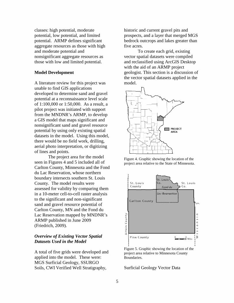
Appendix A: The project’s sand and gravel resource modeling grid inputs prior to being weighted.

Figure 11. MGS surficial geology grid displayed by their sand and gravel ranked index values. These values can be referenced in table 1 for map unit descriptions.

Figure 12. SSURGO soils grid of parent materials displayed by their sand and gravel ranked index values. These values can be referenced in table 2 for map unit descriptions.

Figure 13. CWI Stratigraphy interpolated grid values reclassified to a sand and gravel resource rank (0-10).

Figure 14. Kernel density grid values of identified sand and gravel resources. Density values reclassified to a sand and gravel resource rank (0-10

21

Appendix B. Table and cross-section to better understand the modeling of CWI stratigraphy for this project. Table 11. Extract of the CWI stratigraphy data table displaying the original CWI field headings (no background) and the field headings developed for this project (dark grey). These new field headings were created to calculate a final CWI stratigraphy value (CWI_SFV = SMR*TSM*NONSIGV*OSMR) for each record.

22

Figure 15. Cross-Section Graphic A shows the spatial location of a 3.5 mile line over a 1:24,000 scale USGS topographic map within this project’s area. Additionally Graphic A shows that line transecting 11 CWI well locations which are labeled with their respective unique ids (exp., 549874). That same line in addition to each well’s stratigraphic materials (exp., Sand & Gravel, Clay) is displayed in a geologic cross-section with a vertical exaggeration of 6 seen in Cross-Section Graphic C. In addition, Graphic C displays each well’s CWI final sand and gravel value (exp., 114946 = 330). This value is the sum of all the individual CWI stratigraphy values (CWI_SFV) in a single well. Refer to table 11 on the previous page for how the CWI stratigraphic value is calculated. To better explain the final sand and gravel value calculation examine well number 549874 which is the first well in Cross-Section Graphic C. This well is shown to have 6 line breaks in its well log which implies there are six unique stratigraphic values for that well. All of those records were summed together for a final sand and gravel value of 66. The final sand and gravel value for each well location was applied in an IDW interpolation using ArcGIS Desktop Spatial Analyst shown in Figure 12 of Appendix A. The resulting grid for the cross-section’s geographic area is shown in Cross-Section Graphic B. Darker colors indicate higher sand and gravel values while lighter colors indicate low sand and gravel values.

23

Appendix C. The project’s sand and gravel resource modeling grid inputs after being weighted.

Figure 16. MGS surficial geology grid with applied weight of 8.

Figure 17. SSURGO soils grid with applied weight of 5.

Figure 18. County Well Index modeled grid with applied weight of 3.

Figure 19. Kernel density grid of identified sand and gravel resources with applied weight of 4.

Figure 20. Lakes and outcrops equal 0 (black).

24

Appendix D. Final sand and gravel model grid displayed by stretched values and range of values.

Figure 21. This project’s final sand and gravel model classified by stretched values and description of the calculation applied for the final grid.

Figure 22. This project’s final sand and gravel model classified by a range of values and description of the calculation applied for the final grid.

25

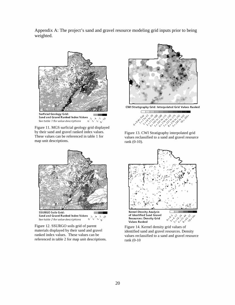
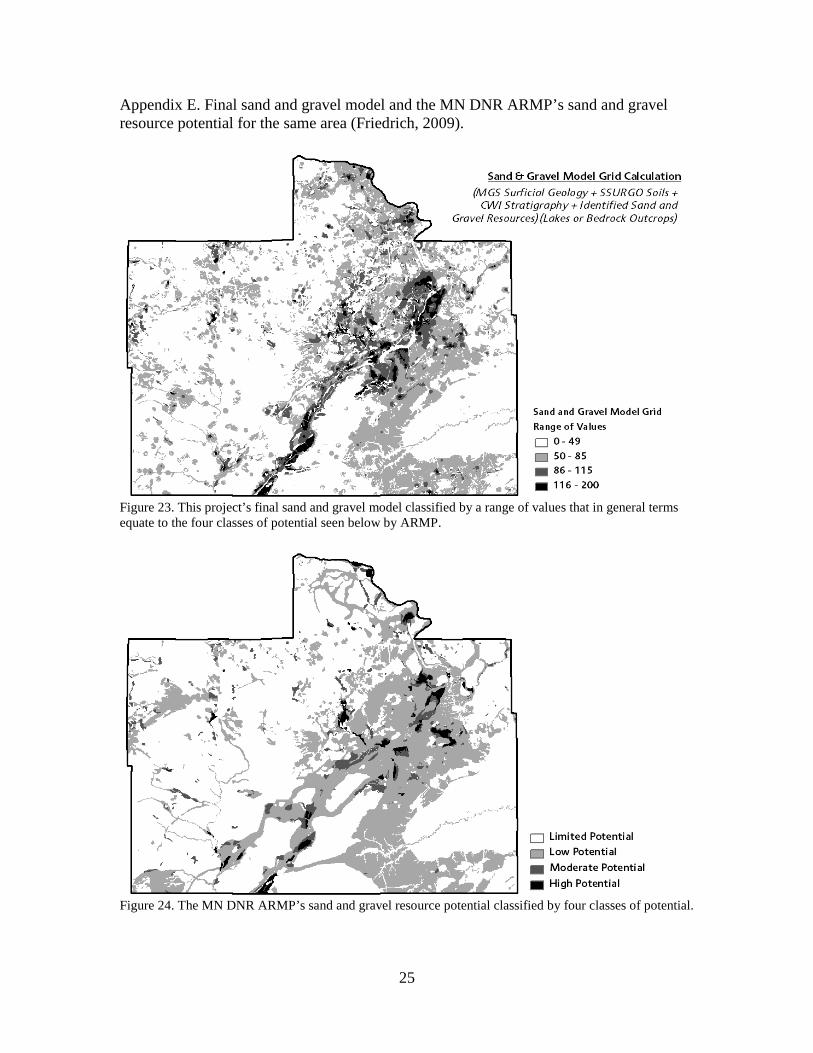
Appendix E. Final sand and gravel model and the MN DNR ARMP’s sand and gravel resource potential for the same area (Friedrich, 2009).

Figure 23. This project’s final sand and gravel model classified by a range of values that in general terms equate to the four classes of potential seen below by ARMP.

Figure 24. The MN DNR ARMP’s sand and gravel resource potential classified by four classes of potential.