Embed Size (px)
DESCRIPTION
Graduate School Quantitative Research Methods Gwilym Pryce [email protected]. Lecture 7: Two Way Tables. Notices:. Register. Aims and Objectives:. Aim: This session introduces methods of examining relationships between categorical variables Objectives: - PowerPoint PPT Presentation
Citation preview

2
Notices:
Register
3
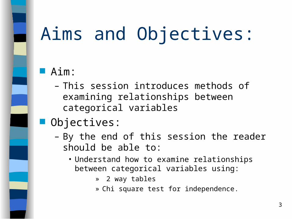
Aims and Objectives:
Aim:– This session introduces methods of examining
relationships between categorical variables Objectives:
– By the end of this session the reader should be able to:
• Understand how to examine relationships between categorical variables using:
» 2 way tables
» Chi square test for independence.
4
Plan:
1. Independent events 2. Contingent events 3. Chi square test for independence 4. Further Study
5
1. Probability of two Independent events occurring If knowing that one event occurs does
not affect the outcome of another event, we say those two outcomes are independent.
And if A and B are independent, and we know the probability of each of them occurring, we can calculate the probability of them both occurring

6
Example: You have a two sided die and a coin, find Pr(1 and H). Answer: ½ x ½ = ¼ Rule: P(A B) = P(A) x P(B)
7
e.g. You have one coin which you toss twice: what’s the probability of getting two heads? Suppose:
• A = 1st toss is a head• B = 2nd toss is a head
– what is the probability of A B? Answer: A and B are independent and
are not disjoint. P(A) = 0.5 and P(B) = 0.5. P (A B) = 0.5 x 0.5 = 0.25.
8
2. Probability of two contingent events occurring If knowing that one event occurs does
change the probability that the other occurs, then two events are not independent and are said to be contingent upon each other
If events are contingent then we can say that there is some kind of relationship between them
So testing for contingency is one way of testing for a relationship
9
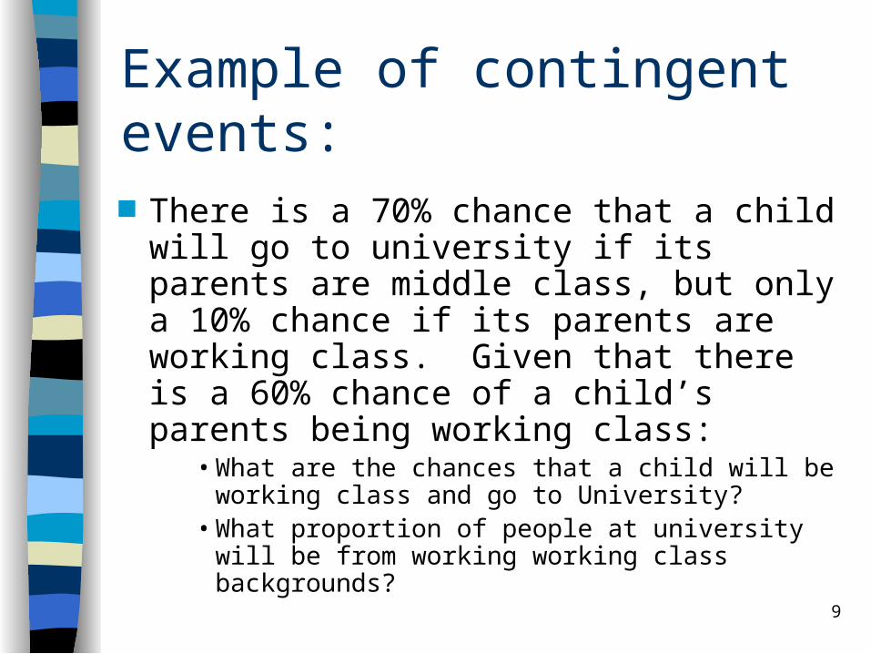
Example of contingent events:
There is a 70% chance that a child will go to university if its parents are middle class, but only a 10% chance if its parents are working class. Given that there is a 60% chance of a child’s parents being working class:
• What are the chances that a child will be working class and go to University?
• What proportion of people at university will be from working working class backgrounds?

10
A tricky one...

11
Working Class
Middle Class

12
6% of all children are both working class and end up going to University
Working Class
Middle Class
13
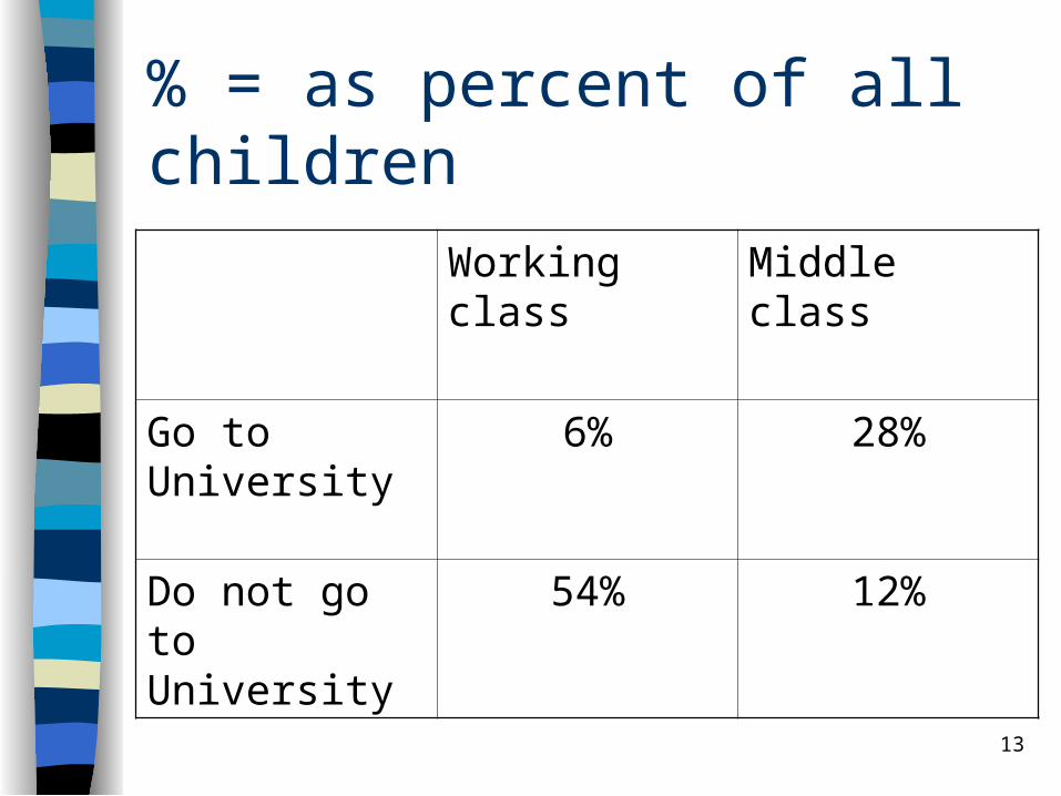
% = as percent of all children
Working class Middle class
Go to University
6% 28%
Do not go to University
54% 12%

14
% at Uni from WC parents?
Of all children, only 32% end up at university (6% WC; 28% MC)
I.e 6 out of every 32 University students are from WC parents:
6/32 = 18.75% of University students are WC

15
Probability theory states that: – if x and y are independent, then the probability of
events x and y simultaneously occurring is simply equal to the product of the two events occurring:
– if x and y are not independent, then:Prob(x y) = Prob(x) Prob(y given that x has occurred)
)(obPr)(obPr)(obPr xxyx

16
Test for independence
We can use these two rules to test whether events are independent– Does the distribution of observations across
possible outcomes resemble the random distribution we would get if events were independent?
– I.e. if we assume independence and calculate the expected number of of cases in each category, do these figures correspond fairly closely to the actual distribution of outcomes found in our data?

17
Example 1: Is there a relationship between social class and education? We might test this by looking at categories in our data of WC, MC, University, no University. Suppose we have 300 observations distributed as follows:
Working class Middle class
Go to University 18 84
Do not go to University 162 36
18
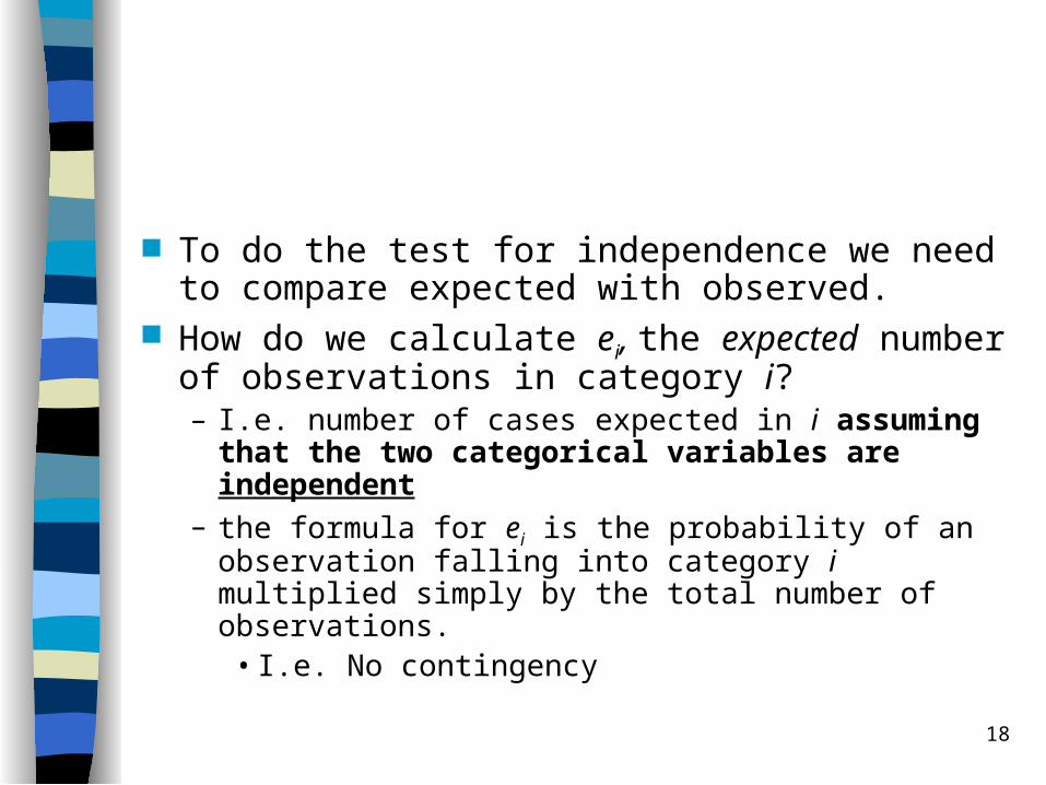
To do the test for independence we need to compare expected with observed.
How do we calculate ei, the expected number of observations in category i?– I.e. number of cases expected in i assuming that
the two categorical variables are independent– the formula for ei is the probability of an
observation falling into category i multiplied simply by the total number of observations.
• I.e. No contingency

19
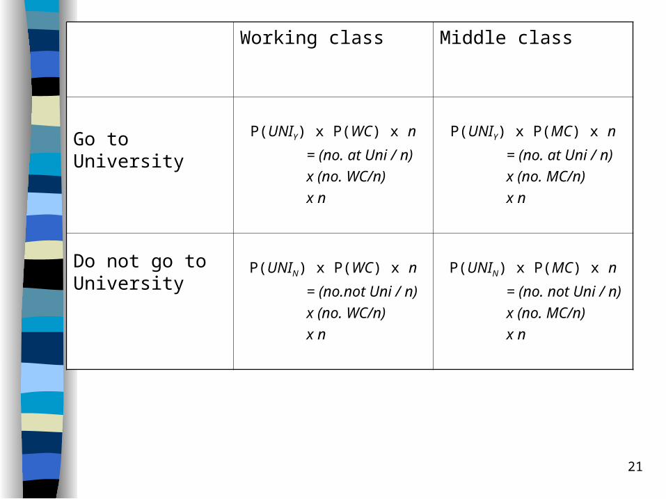
So, if UNIY or UNIN and WC or MC are independent (i.e. assuming H0) then:Prob(UNIY WC) = Prob(UNIY)Prob(WC)
– so the expected number of cases for each of the four mutually exclusive categories are as follows:
Working class Middle class
Go to University P(UNIY) x P(WC) x n P(UNIY) x P(MC) x n
Do not go to University
P(UNIN) x P(WC) x n P(UNIN) x P(MC) x n
20
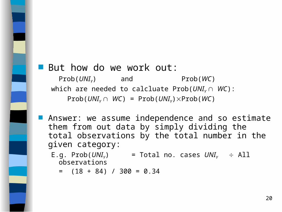
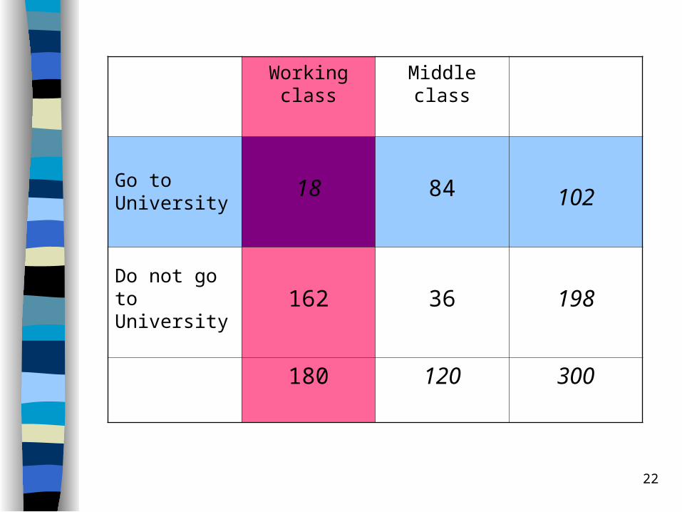
But how do we work out:Prob(UNIY) and Prob(WC)
which are needed to calcluate Prob(UNIY WC):
Prob(UNIY WC) = Prob(UNIY)Prob(WC)
Answer: we assume independence and so estimate them from out data by simply dividing the total observations by the total number in the given category:E.g. Prob(UNIY) = Total no. cases UNIY All observations = (18 + 84) / 300 = 0.34
21
Working class Middle class
Go to University P(UNIY) x P(WC) x n
= (no. at Uni / n)
x (no. WC/n)
x n
P(UNIY) x P(MC) x n
= (no. at Uni / n)
x (no. MC/n)
x n
Do not go to University
P(UNIN) x P(WC) x n
= (no.not Uni / n)
x (no. WC/n)
x n
P(UNIN) x P(MC) x n
= (no. not Uni / n)
x (no. MC/n)
x n
22
Working class Middle class
Go to University
18 84 102
Do not go to University 162 36 198
180 120 300
23
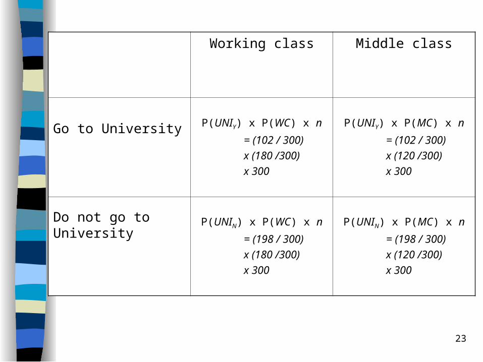
Working class Middle class
Go to University P(UNIY) x P(WC) x n
= (102 / 300)
x (180 /300)
x 300
P(UNIY) x P(MC) x n
= (102 / 300)
x (120 /300)
x 300
Do not go to University
P(UNIN) x P(WC) x n
= (198 / 300)
x (180 /300)
x 300
P(UNIN) x P(MC) x n
= (198 / 300)
x (120 /300)
x 300

24
Expected count in each category:
Working class Middle class
Go to University
(102 / 300) x (180 /300) x 300
= .34 x .6 x 300 = 61.2
(102 / 300) x (120 /300) x 300
= .34 x .4 x 300 = 40.8
Do not go to University
(198 / 300) x (180 /300) x 300
= .66 x .6 x 300 = 118.8
(198 / 300) x (120 /300) x 300
= .66 x .4 x 300 = 79.2
25
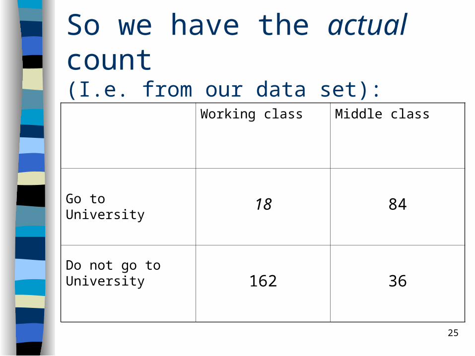
So we have the actual count (I.e. from our data set):
Working class Middle class
Go to University 18 84
Do not go to University 162 36
26
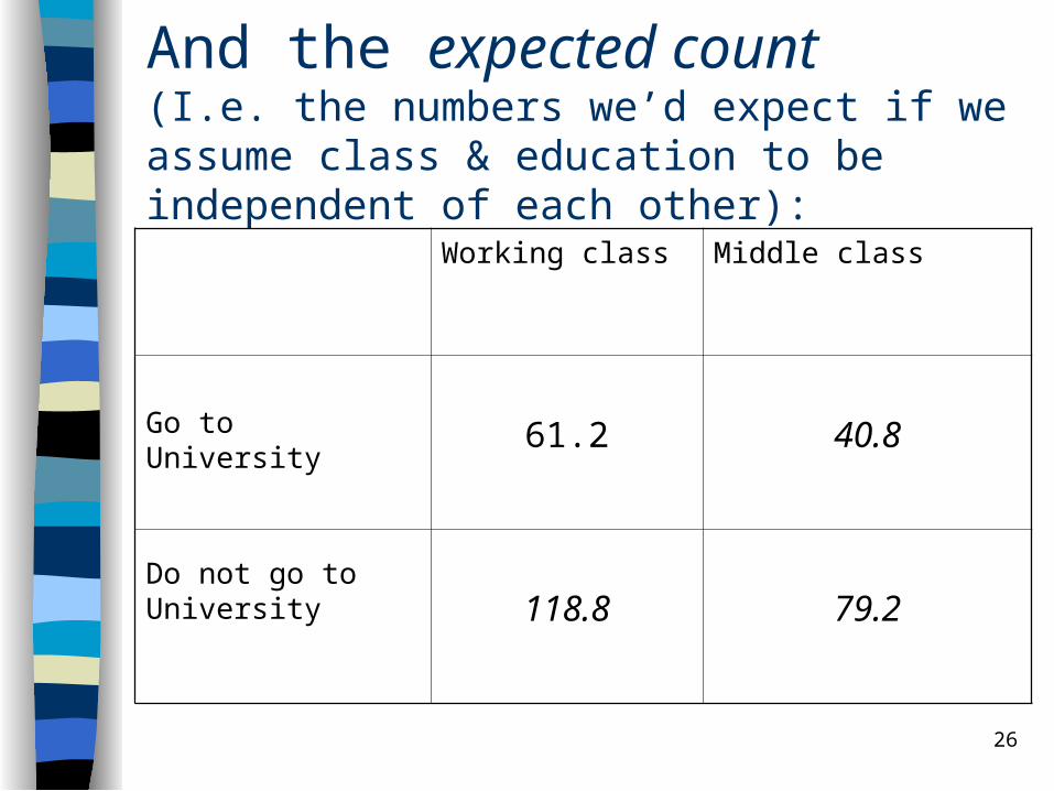
And the expected count (I.e. the numbers we’d expect if we assume class & education to be independent of each other):
Working class Middle class
Go to University 61.2 40.8
Do not go to University 118.8 79.2
27
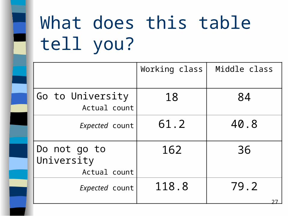
What does this table tell you?
Working class Middle class
Go to UniversityActual count
18 84
Expected count 61.2 40.8
Do not go to UniversityActual count
162 36
Expected count 118.8 79.2
28
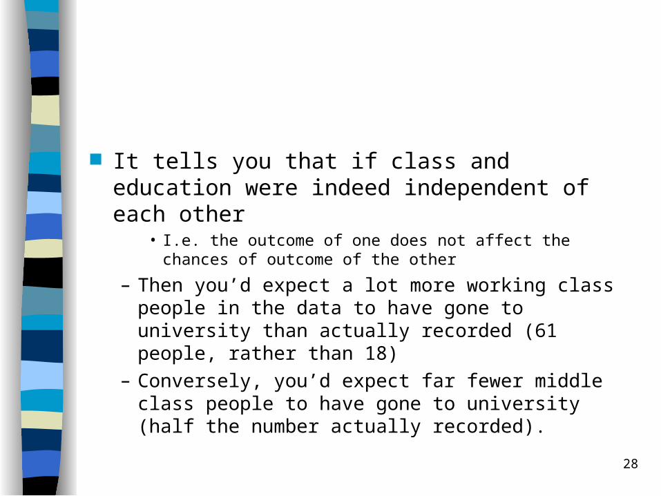
It tells you that if class and education were indeed independent of each other
• I.e. the outcome of one does not affect the chances of outcome of the other
– Then you’d expect a lot more working class people in the data to have gone to university than actually recorded (61 people, rather than 18)
– Conversely, you’d expect far fewer middle class people to have gone to university (half the number actually recorded).
29
But remember, all this is based on a sample, not the entire population…
Q/ Is this discrepancy due to sampling variation alone or does it indicate that we must reject the assumption of independence?
30
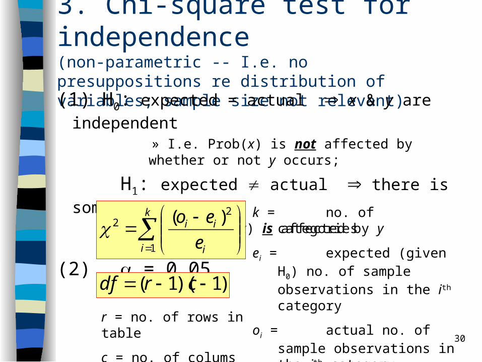
3. Chi-square test for independence (non-parametric -- I.e. no presuppositions re distribution of variables; sample size not relevant)
(1) H0: expected = actual x & y are independent
» I.e. Prob(x) is not affected by whether or not y occurs;
H1: expected actual there is some
relationship»I.e. Prob(x) is affected by y occurring.
(2) = 0.05
k
i i
ii
e
eo
1
22 )(
k = no. of categories
ei = expected (given H0) no. of sample observations in the ith category
oi = actual no. of sample observations in the ith category
d = no. of parameters that have to be estimated from the sample data.
)1)(1( crdf
r = no. of rows in table
c = no. of colums “ “

31
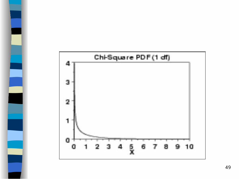
Chi-square distribution changes shape for different df:

32
(3) Reject H0 iff P <
(4) Calculate P:• P = Prob(2 > 2
c)
– N.B. Chi-square tests are always an upper tail test 2 Tables: are usually set up like a t-table with df down the
side, and the probabilities listed along the top row, with values of 2
c actually in the body of the table. So look up 2c
in the body of the table for the relevant df and then find the upper tail probability that heads that column.
– SPSS: - CDF.CHISQ(2c,df) calculates Prob(2 < 2
c), so use the following syntax:
» COMPUTE chi_prob = 1 - CDF.CHISQ(2c,df).
» EXECUTE.
33
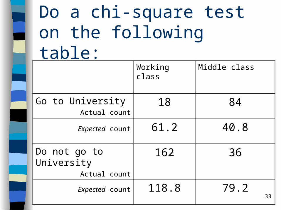
Do a chi-square test on the following table:
Working class Middle class
Go to UniversityActual count
18 84
Expected count 61.2 40.8
Do not go to UniversityActual count
162 36
Expected count 118.8 79.2
34
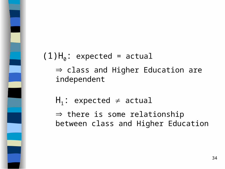
(1) H0: expected = actual
class and Higher Education are independent
H1: expected actual
there is some relationship between class and Higher Education
35
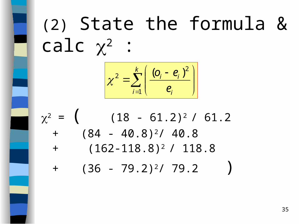
(2) State the formula & calc 2 :
2 = ( (18 - 61.2)2 / 61.2
+ (84 - 40.8)2/ 40.8+ (162-118.8)2 / 118.8
+ (36 - 79.2)2/ 79.2 )
k
i i
ii
e
eo
1
22 )(
36
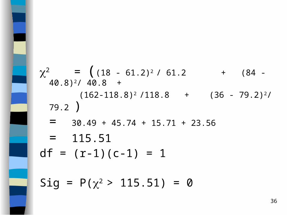
2 = ((18 - 61.2)2 / 61.2 + (84 - 40.8)2/ 40.8 +
(162-118.8)2 /118.8 + (36 - 79.2)2/ 79.2 )= 30.49 + 45.74 + 15.71 + 23.56
= 115.51df = (r-1)(c-1) = 1
Sig = P(2 > 115.51) = 0

37
(3) Reject H0 iff P <
(4) Calculate P:
COMPUTE chi_prob = 1 - CDF.CHISQ(115.51,1).
EXECUTE.
Sig = P(2 > 115.51) = 0
Reject H0
38
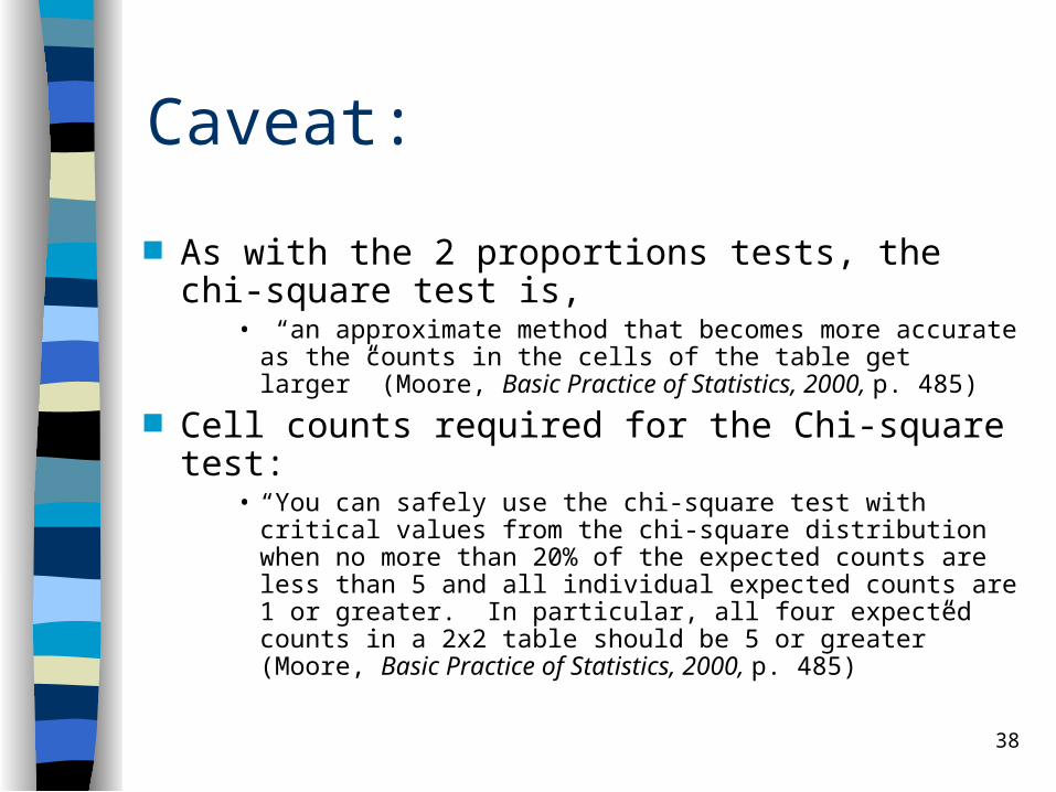
Caveat:
As with the 2 proportions tests, the chi-square test is,
• “an approximate method that becomes more accurate as the counts in the cells of the table get larger” (Moore, Basic Practice of Statistics, 2000, p. 485)
Cell counts required for the Chi-square test:• “You can safely use the chi-square test with critical
values from the chi-square distribution when no more than 20% of the expected counts are less than 5 and all individual expected counts are 1 or greater. In particular, all four expected counts in a 2x2 table should be 5 or greater” (Moore, Basic Practice of Statistics, 2000, p. 485)
39
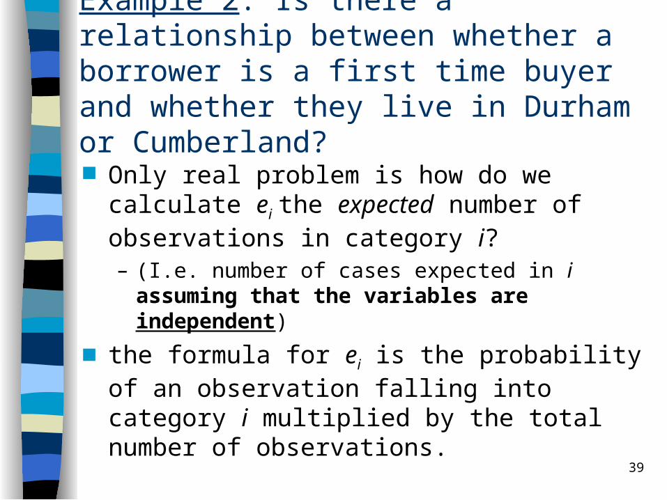
Example 2: Is there a relationship between whether a borrower is a first time buyer and whether they live in Durham or Cumberland?
Only real problem is how do we calculate ei the expected number of observations in category i?– (I.e. number of cases expected in i assuming that
the variables are independent)
the formula for ei is the probability of an observation falling into category i multiplied by the total number of observations.
40
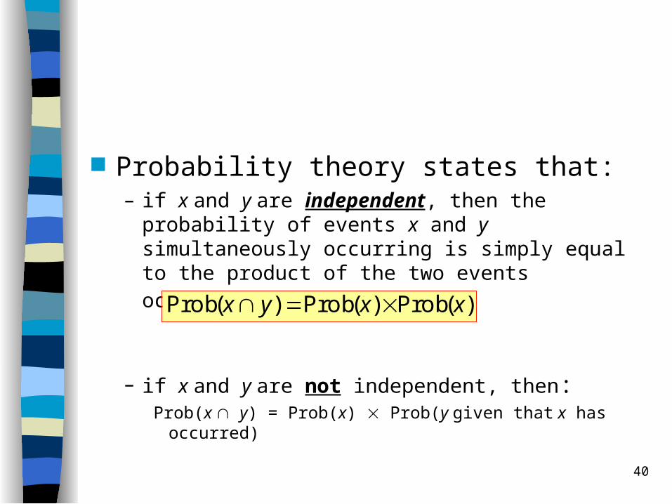
Probability theory states that: – if x and y are independent, then the probability of
events x and y simultaneously occurring is simply equal to the product of the two events occurring:
– if x and y are not independent, then:Prob(x y) = Prob(x) Prob(y given that x has occurred)
)(obPr)(obPr)(obPr xxyx

41
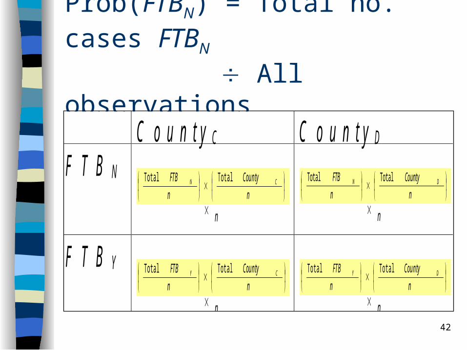
So, if FTBY or N and CountyD or C are independent (i.e. assuming H0) then:Prob(FTBY CountyD) = Prob(FTBY)Prob(CountyD)
so the expected number of cases for each of the four mutually exclusive categories are as follows:
42
Prob(FTBN) = Total no. cases FTBN
All observations
C o u n t y C C o u n t y D
F T B N
n
County
n
FTB CN Total Total
n
n
County
n
FTB DN Total Total
n
F T B Y
n
County
n
FTB CY Total Total
n
n
County
n
FTB DY Total Total
n

43
44
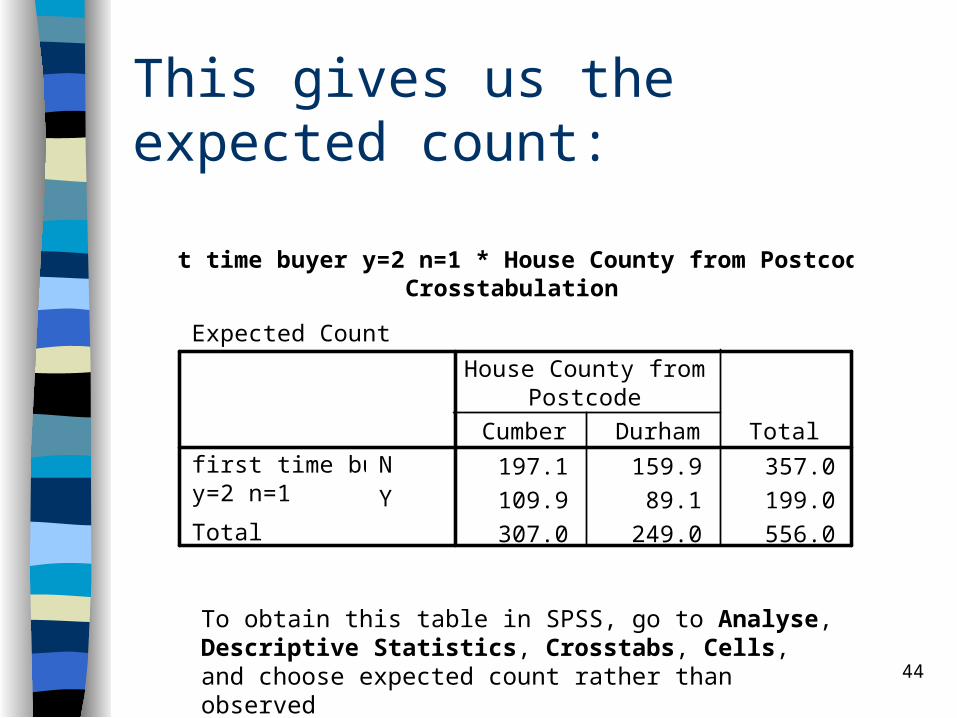
This gives us the expected count:
first time buyer y=2 n=1 * House County from Postcode Crosstabulation
Expected Count
197.1 159.9 357.0
109.9 89.1 199.0
307.0 249.0 556.0
N
Y
first time buyery=2 n=1
Total
Cumber Durham
House County fromPostcode
Total
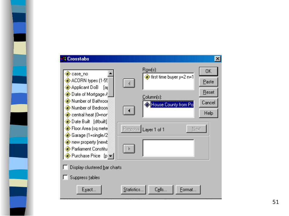
To obtain this table in SPSS, go to Analyse, Descriptive Statistics, Crosstabs, Cells, and choose expected count rather than observed

45
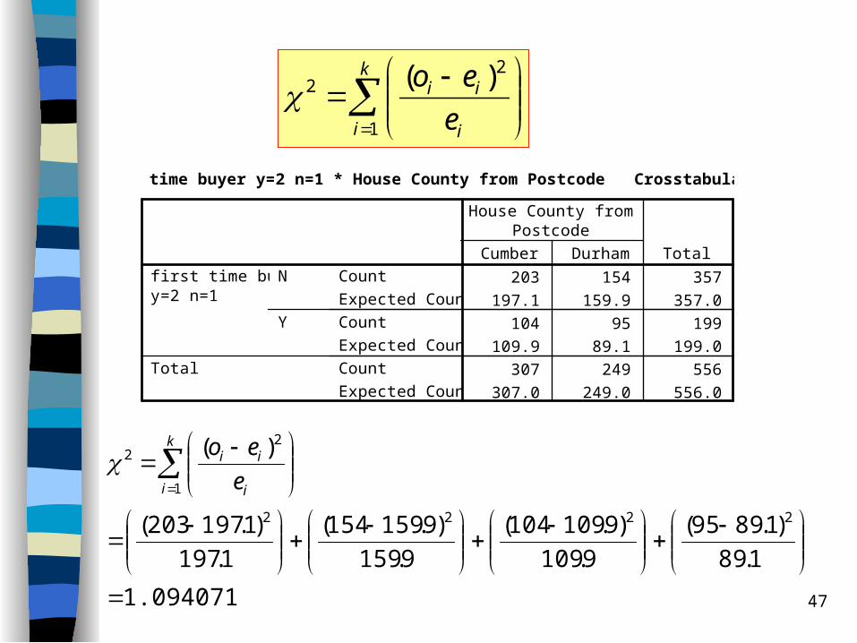
first time buyer y=2 n=1 * House County from Postcode Crosstabulation
203 154 357
197.1 159.9 357.0
104 95 199
109.9 89.1 199.0
307 249 556
307.0 249.0 556.0
Count
Expected Count
Count
Expected Count
Count
Expected Count
N
Y
first time buyery=2 n=1
Total
Cumber Durham
House County fromPostcode
Total
46
What does this table tell you? – Does it suggest that the probability of being
an FTB independent of location?– Or does it suggest that the two factors are
contingent on each other in some way?– Can it tell you anything about the direction
of causation?– What about sampling variation?
47
first time buyer y=2 n=1 * House County from Postcode Crosstabulation
203 154 357
197.1 159.9 357.0
104 95 199
109.9 89.1 199.0
307 249 556
307.0 249.0 556.0
Count
Expected Count
Count
Expected Count
Count
Expected Count
N
Y
first time buyery=2 n=1
Total
Cumber Durham
House County fromPostcode
Total
k
i i
ii
e
eo
1
22 )(
1.094071
1.89
)1.8995(
9.109
)9.109104(
9.159
)9.159154(
1.197
)1.197203(
)(
2222
1
22
k
i i
ii
e
eo

48
Summary of Hypothesis test:
– (1) H0: FTB and County are independent
H1: there is some relationship– (2) = 0.05
– (3) Reject H0 iff P < – (4) Calculate P:
• P = Prob(2 > 2c) = 0.29557 Do not reject H0
I.e. if we were to reject H0, there would be a 1 in 3 chance of us rejecting it incorrectly, and so we cannot do so. In other words, FTB and County are independent.
1.094071
)(
1
22
k
i i
ii
e
eo
1
)12)(12(
)1)(1(
crdf
49

50
Contingency Tables in SPSS:
51
52
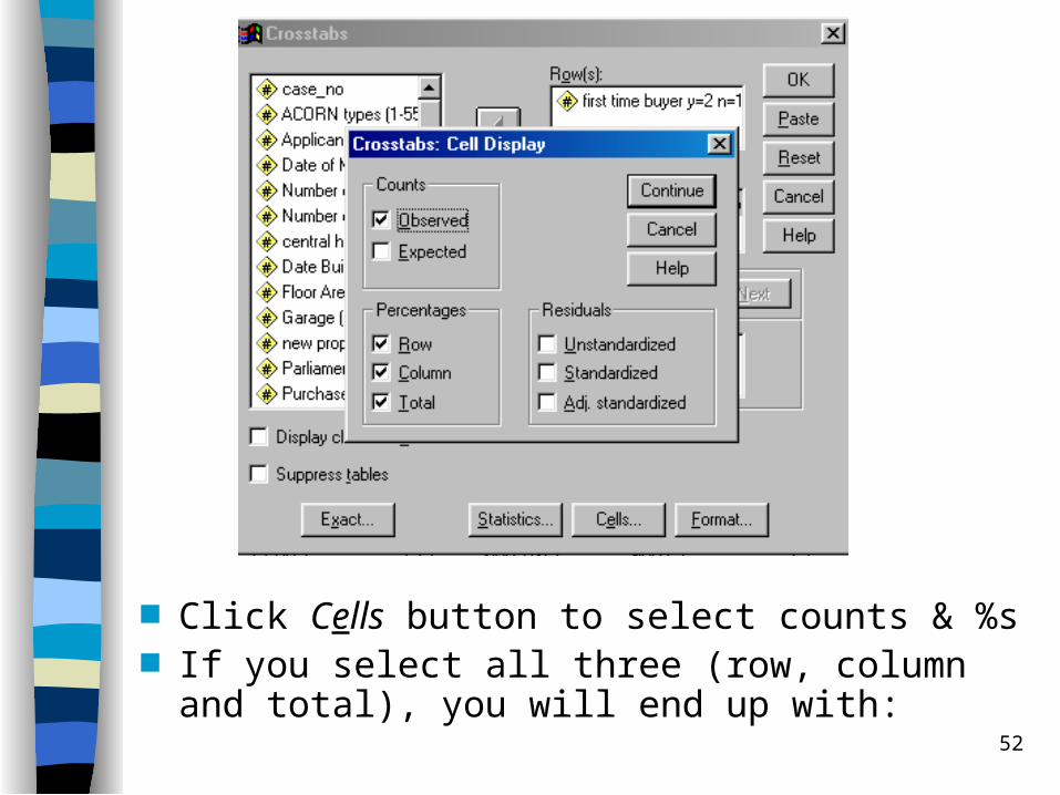
Click Cells button to select counts & %s If you select all three (row, column and total),
you will end up with:
53
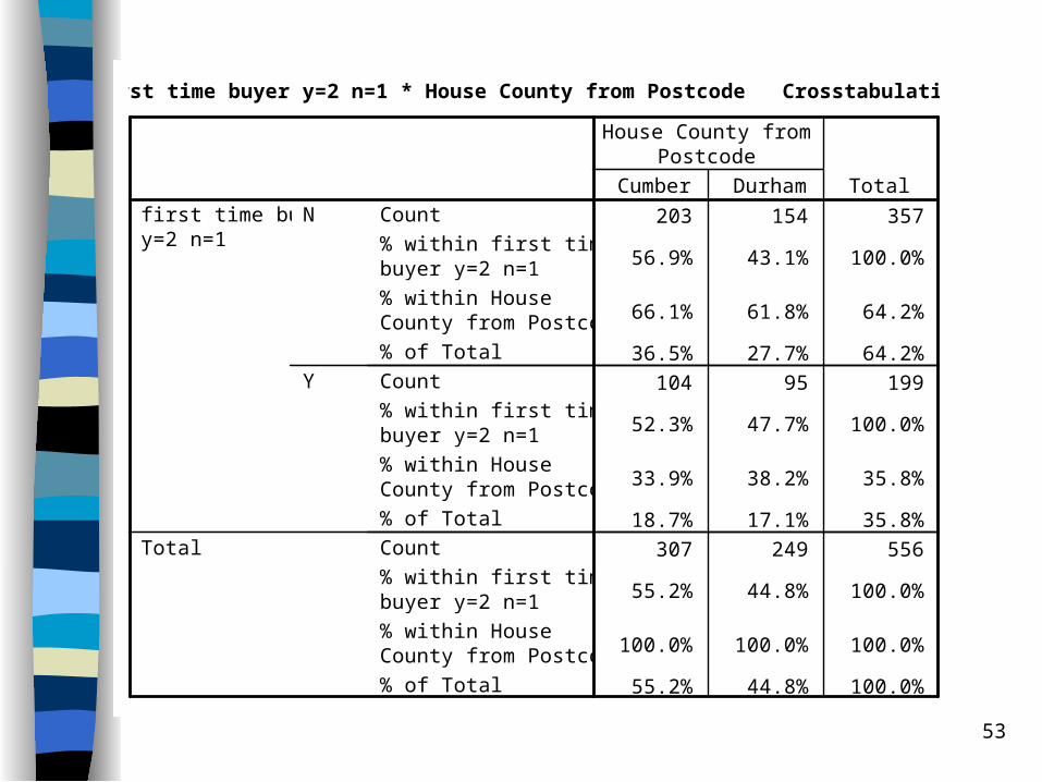
first time buyer y=2 n=1 * House County from Postcode Crosstabulation
203 154 357
56.9% 43.1% 100.0%
66.1% 61.8% 64.2%
36.5% 27.7% 64.2%
104 95 199
52.3% 47.7% 100.0%
33.9% 38.2% 35.8%
18.7% 17.1% 35.8%
307 249 556
55.2% 44.8% 100.0%
100.0% 100.0% 100.0%
55.2% 44.8% 100.0%
Count
% within first timebuyer y=2 n=1
% within HouseCounty from Postcode
% of Total
Count
% within first timebuyer y=2 n=1
% within HouseCounty from Postcode
% of Total
Count
% within first timebuyer y=2 n=1
% within HouseCounty from Postcode
% of Total
N
Y
first time buyery=2 n=1
Total
Cumber Durham
House County fromPostcode
Total
54
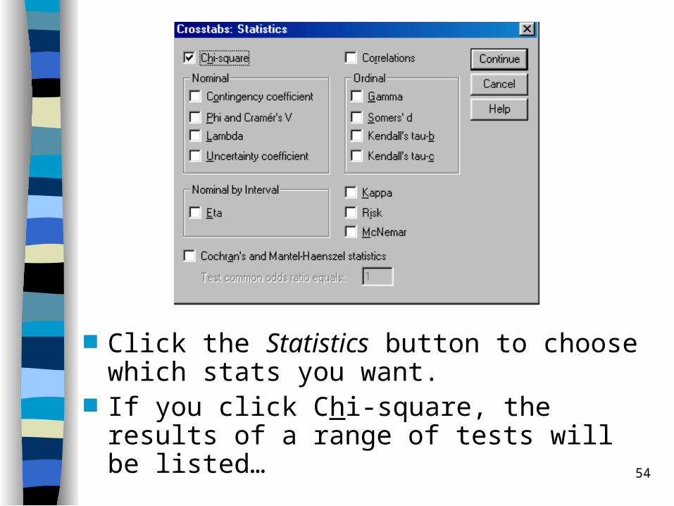
Click the Statistics button to choose which stats you want.
If you click Chi-square, the results of a range of tests will be listed…

55
We have been calculating the Pearson Chi-square:
Chi-Square Tests
1.094b 1 .296
.916 1 .339
1.093 1 .296
.328 .169
1.092 1 .296
556
Pearson Chi-Square
Continuity Correctiona
Likelihood Ratio
Fisher's Exact Test
Linear-by-LinearAssociation
N of Valid Cases
Value dfAsymp. Sig.
(2-sided)Exact Sig.(2-sided)
Exact Sig.(1-sided)
Computed only for a 2x2 tablea.
0 cells (.0%) have expected count less than 5. The minimum expected count is89.12.
b.
56
4. For further study:
The Pearson Chi square test only tests for the existence of a relationship
• It tells you little about the strength of the relationship
SPSS includes a raft of measures that try to measure the level of association between categorical variables.
• Click on the name of one of the statistics and SPSS will give you a brief definition (see below)
• In the lab exercises, take a look at these statistics and copy and paste the definitions along side your answers
– Right click on the definition and select Copy. Then open up a Word document and paste along with your output.
57
Nominal variables: Contingency coefficient:
• “A measure of association based on chi-square. The value ranges between zero and 1, with zero indicating no association between the row and column variables and values close to 1 indicating a high degree of association between the variables. The maximum value possible depends on the number of rows and columns in a table.”
Phi and Cramer’s V:• “Phi is a chi-square based measure of association that involves dividing the
chi-square statistic by the sample size and taking the square root of the result. Cramer's V is a measure of association based on chi-square.”
Lambda:• “A measure of association which reflects the proportional reduction in error
when values of the independent variable are used to predict values of the dependent variable. A value of 1 means that the independent variable perfectly predicts the dependent variable. A value of 0 means that the independent variable is no help in predicting the dependent variable.”
Uncertainty coefficient:• “A measure of association that indicates the proportional reduction in errror
when values of one variable are used to predict values of the other variable. For example, a value of 0.83 indicates that knowledge of one variable reduces error in predicting values of the other variable by 83%. The program calculates both symmetric and asymmetric versions of the uncertainty coefficient.”

58
Ordinal Variables: Gamma:
• A symmetric measure of association between two ordinal variables that ranges between negative 1 and 1. Values close to an absolute value of 1 indicate a strong relationship between the two variables. Values close to zero indicate little or no relationship. For 2-way tables, zero-order gammas are displayed. For 3-way to n-way tables, conditional gammas are displayed.
Somers’ d:• “A measure of association between two ordinal variables that ranges from -1 to 1.
Values close to an absolute value of 1 indicate a strong relationship between the two variables, and values close to 0 indicate little or no relationship between the variables. Somers' d is an asymmetric extension of gamma that differs only in the inclusion of the number of pairs not tied on the independent variable. A symmetric version of this statistic is also calculated.”
Kendall’s tau-b:• “A nonparametric measure of association for ordinal or ranked variables that take
ties into account. The sign of the coefficient indicates the direction of the relationship, and its absolute value indicates the strength, with larger absolute values indicating stronger relationships. Possible values range from -1 to 1, but a value of -1 or +1 can only be obtained from square tables.”
Kendall’s tau-c:• “A nonparametric measure of association for ordinal variables that ignores ties. The
sign of the coefficient indicates the direction of the relationship, and its absolute value indicates the strength, with larger absolute values indicating stronger relationships. Possible values range from -1 to 1, but a value of -1 or +1 can only be obtained from square tables.”
59
Correlations:
Pearson correlation coefficient r• “a measure of linear association between two variables”
Spearman correlation coefficient• “a measure of association between rank orders. Values
of both range between -1 (a perfect negative relationship) and +1 (a perfect positive relationship). A value of 0 indicates no linear relationship.”

60
When you have a dependent variable measured on an interval scale & an independent variable with a limited number of categories:
Eta:– “A measure of association that ranges from 0 to 1, with 0 indicating no
assoication between the row and column variables and values close to 1 indicating a high degree of association. Eta is appropriate for a dependent variable measured on an interval scale (e.g., income) and an independent variable with a limited number of categories (e.g., gender). Two eta values are computed: one treats the row variable as the interval variable; the other treats the column variable as the interval variable.”