Graph layering by promotion of nodes

Discrete Applied Mathematics 154 (2006) 848–860www.elsevier.com/locate/dam

Graph layering by promotion of nodesNikola S. Nikolov∗, Alexandre Tarassov

Department of Computer Science and Information Systems, University of Limerick, Ireland

Received 29 November 2002; received in revised form 4 December 2003; accepted 31 May 2005Available online 15 November 2005

Abstract

This work contributes to the wide research area of visualization of hierarchical graphs. We present a new polynomial-time heuristicwhich can be integrated into the Sugiyama method for drawing hierarchical graphs. Our heuristic, which we call Promote Layering(PL), is applied to the output of the layering phase of the Sugiyama method. PL is a simple and easy to implement algorithm whichdecreases the number of so-called dummy (or virtual) nodes in a layered directed acyclic graph. In particular, we propose applyingPL after the longest-path layering algorithm and we present an extensive empirical evaluation of this layering technique.© 2005 Elsevier B.V. All rights reserved.

Keywords: Graph drawing; Layered directed acyclic graph; Layering algorithm

1. Introduction

To layer a directed acyclic graph (DAG) is to partition its node set into subsets such that nodes connected by adirected path belong to different subsets. In addition, subsets are assigned integer ranks such that for each edge therank of the subset that contains the target of the edge is less than the rank of the subset that contains its source. Such anordered partition of the node set of a DAG is known as a layering and the corresponding subsets are called layers. EachDAG allows at least one layering; a DAG with a given layering is called a layered DAG. Most often layered DAGs arevisualized by placing the DAG nodes on parallel horizontal levels such that each layer occupies a single level, differentlayers occupy different levels, and all edges point in the same direction. Fig. 1 gives an example of two alternative waysto layer the same DAG.

In this work, we consider the graph layering problem in the context of DAG visualization. In the research area knownas graph drawing there have been recognized a few different methods for drawing DAGs. The more recent two area magnetic field model introduced by Sugiyama and Misue [15] and an evolutionary algorithm by Utech et al. [18].While potentially these two are an area of fruitful future research, an earlier method, widely known as the Sugiyama (orSTT) method [16], has received most of the research attention and has become a standard method for drawing DAGs.The Sugiyama method is a three phase algorithmic framework, originally proposed by Sugiyama et al. [16], and alsobased on work by Warfield [19] and Carpano [2]. At its first phase the nodes of a DAG are partitioned into layers and

∗ Corresponding author. CSIS Department, University of Limerick, Limerick, Ireland.E-mail addresses: [email protected] (N.S. Nikolov), [email protected] (A. Tarassov).

0166-218X/$ - see front matter © 2005 Elsevier B.V. All rights reserved.doi:10.1016/j.dam.2005.05.023

http://www.elsevier.com/locate/dam

mailto:[email protected]

mailto:[email protected]

N.S. Nikolov, A. Tarassov / Discrete Applied Mathematics 154 (2006) 848–860 849

(a) (b)

Fig. 1. Two alternative layerings of the same DAG. Each layer occupies a horizontal level marked by a dashed line. All edges point downwards.

each layer is assigned to a horizontal level; at the second phase the nodes are ordered within each layer; and at thefinal third phase the x- and y-coordinates of all nodes and the eventual edge bends are precisely tuned. In this paper,we propose a heuristic, called Promote Layering (PL), that can be applied at the end of the first phase and before thesecond phase for improving the characteristics of an already found layering.

If there are no additional requirements it is not hard to find a layering of a DAG. Classical graph algorithms such asbreadth-first search, depth-first search and algorithms for finding a minimum spanning tree can be easily modified topartition the node set of a DAG into layers. However, normally it is desirable to take into account a number of additionalcriteria when computing a layering [5]. It might be desirable to keep the number of layers and the maximum numberof nodes per layer within certain bounds. Also, for the clarity of the final drawing, it is preferable to partition the nodeset into layers so that long edges spanning several layers are kept to a small number. A large number of long edgesalso significantly slows down the algorithms applied at the next two phases of the Sugiyama method. It might be alsoa good idea to find a layering with low edge density between adjacent horizontal levels in the corresponding drawing.The PL heuristic that we propose in this paper can be used for achieving a layering with short edges and, as we haveobserved experimentally, low edge density.

The paper is organized as follows. The Section 2 introduces the basic terminology required for discussing graphlayering further. In Section 3, we briefly describe the known algorithms for partitioning the node set of a DAGinto layers. Section 4 introduces our new layering improvement heuristic, PL. Then in Section 5 we report ex-perimental results of applying PL to about 8000 DAGs taken from various benchmark graph databases and com-pare it to other layering techniques. In Section 6, we draw conclusions from this work and outline directions forfurther work.

2. Preliminaries

Consider a DAG G= (V , E) with a set of nodes V and a set of edges E. The in-degree of node v, denoted by d−(v),is the number of edges with a target v, and the out-degree of v, denoted by d+(v), is the number of edges with a sourcev. We denote the set of all immediate predecessors of node v by N−G(v), and the set of all immediate successors ofnode v by N+G(v). That is, N−G(v)= {u : (u, v) ∈ E} and N+G(v)= {u : (v, u) ∈ E}.

Let L= {L0, L1, . . . , Lh} be a partition of the node set of G into h�1 subsets such that if (u, v) ∈ E with u ∈ Lj

and v ∈ Li then i < j . L is called a layering of G and the sets L0, L1, . . . , Lh are called layers. A DAG with a layeringis called a layered DAG. In the remainder of this paper, we assume that in a visual representation of a layered DAG allnodes in layer Li are placed on the horizontal level with an y-coordinate i. Thus, we say that Lj is above Li and Li isbelow Lj if i < j .

Let l(u,L) denote the number of a layer which contains node u ∈ V , i.e., l(u,L) = i if and only if u ∈ Li .Then the span of edge e = (u, v) in layering L is defined as s(e,L) = l(u,L) − l(v,L). Clearly, s(e,L)�1 for

850 N.S. Nikolov, A. Tarassov / Discrete Applied Mathematics 154 (2006) 848–860

L 2

L 1

L 0

L 3

L 3

L 2

L 1

L 0

L 4

(a) (b)

Fig. 2. The drawings from Fig. 1 with introduced dummy nodes which subdivide long edges. Dummy nodes are represented by transparent squares.(a) A layering with 4 layers and 5 dummy nodes; (b) a layering with 5 layers and 4 dummy nodes.

each e ∈ E; edges with a span greater than 1 are long edges. A layering of G is proper if s(e,L) = 1 for eache ∈ E, i.e. if there are no long edges. The layering found by a layering algorithm might not be proper because onlya small fraction of DAGs can be layered properly and also because a proper layering may not satisfy other layeringrequirements.

In the Sugiyama method for drawing DAGs, the node ordering algorithms applied after the layering phase assumethat their input is a DAG with a proper layering. Thus, if the layering found at the layering phase is not proper then itmust be transformed to a proper one. Normally, this is done by introducing so-called dummy nodes which subdividelong edges (see, the illustration in Fig. 2). Formally, let e = (u, v) be an edge with l(u,L) = j and l(v,L) = i ands(e,L)= j − i > 1. Then we add dummy nodes di+1

e , di+2e , . . . , d

j−1e to layers Li+1, Li+2, . . . , Lj−1, respectively,

and we replace edge e by the path (u, dj−1e , . . . , di+1

e , v). To distinguish the original nodes of a DAG from the dummynodes we refer to the former as regular nodes. We also denote the set of all dummy nodes introduced to a layered DAGG with a layering L by D(G,L). Clearly,

|D(G,L)| =∑

e∈Es(e,L)− |E|.

It is desirable that |D(G,L)| is as small as possible because a large number of dummy nodes significantly slowdown the node ordering phase of the Sugiyama method. Thus, one of the goals of a layering algorithm should be to finda layering with as few as possible dummy nodes. There are also aesthetic reasons for keeping the number of dummynodes small. A layered DAG with a small number of dummy nodes would also have a small number of undesirablelong edges and edge bends.

Other parameters of a layering which reflect on the quality of the drawing are the width and the height of alayering and the edge density between adjacent horizontal levels. The height of a layering is the number of lay-ers, and the width is the maximum number of nodes in a layer. Usually these two parameters are used to ap-proximate the dimensions of the final drawing. When measuring the width of a layering the contribution of thedummy nodes may or may not be taken into account. A more precise definition of the layering width takes intoaccount both variable node widths and the contribution of the dummy nodes [1,8]. The area of a layering, usedto approximate the area of the final drawing, is defined as the product of the layering width and the layeringheight.

The edge density between horizontal levels i and j with i < j is defined as the number of edges (u, v) with u ∈Lj ∪ Lj+1 ∪ · · · ∪ Lh and v ∈ L0 ∪ L1 ∪ · · · ∪ Li . The edge density of a layered DAG is the maximum edge densitybetween adjacent layers (horizontal levels). Naturally, drawings with low maximum and average edge density are clearand easier to comprehend.

In the next section we review the known layering algorithms and discuss the quality of layerings found by them.


3. Existing layering algorithms

At present there are two groups of layering algorithms which find a layering of a DAG subject to some of theabove criteria. The first group of algorithms are adopted from the area of static precedence-constrained multiprocessorscheduling. They produce layerings with either the minimum height or a specified maximum number of nodes per layer.The second group of algorithms employ network simplex and branch-and-cut techniques, respectively, for minimizingthe number of dummy nodes.

3.1. List scheduling algorithms

The precedence-constrained multiprocessor scheduling problem is the problem of scheduling n causally relatedtasks (which represent a parallel program) on m processors with the goal of minimizing the completion time of theparallel program. This problem is also known as static scheduling because all the tasks are given in advance andthe schedule must be constructed prior executing any of them. A simplified version of this problem, where all thetasks have the same computational cost and the communication time between tasks is neglected, is equivalent to theproblem of finding a layering of a DAG with at most m nodes per layer and the minimum number of layers. Thus, theearliest static scheduling algorithms which deal with simplified models have also found an application as DAG layeringalgorithms.

Most of the static scheduling algorithms are variations of a generic list scheduling technique which consists of twomain steps:

(1) build a scheduling list which contains all the tasks;(2) while the scheduling list is not empty remove the first task from it and schedule it for execution on a processor

which allows the earliest start-time.

There are two list scheduling algorithms that have been widely employed as layering algorithms. The first one isthe longest-path algorithm which solves the static scheduling problem for m = ∞. Let � be the number of nodesin the longest directed path in a DAG. The longest-path algorithm builds the scheduling list by assigning prior-ity � to the nodes without outgoing edges. If all immediate successors of a node have been assigned a prioritythen that node is assigned the lowest of the priorities of its immediate successors minus one. This is repeateduntil all nodes are assigned a priority. The nodes with the same priority k form layer L�−k . The advantages ofthe longest-path algorithm are its simplicity and its linear time complexity. It also produces layerings with theminimum height. However, it performs very poorly in terms of drawing area, number of dummy nodes and edge density[9].

The second list scheduling algorithm used for DAG layering is the Coffman–Graham algorithm [3] which is basedon an earlier algorithm by Hu [10]. It approximately solves the static scheduling problem for m <∞ which is NP-hard [17]. The technique used for building the scheduling list is more complex than the one used by the longest-pathalgorithm. The worst-case time complexity of the Coffman–Graham algorithm is O(|V |2). It guarantees a layeringwith at most m nodes per layer and in the worst case the height of the layering may become close to twice the op-timal height [3]. It has been observed that Coffman–Graham layerings have a large amount of dummy nodes andwhen they are taken into account the area of the layerings can be even worse than the area of the longest-pathlayerings [9]. We do not describe the Coffman–Graham algorithm in detail in this paper. It can be found in theoriginal publication of Coffman and Graham [3] as well as in several scheduling and graph drawing publications[5,11].

It can be noted that since the introduction of the Coffman–Graham algorithm a large number of alternative listscheduling algorithms have been proposed for solving variations of the static scheduling problem. In addition, therehave been proposed alternatives to list scheduling. Most of them assume a more complex static scheduling model whichis closer to real scheduling problems and is not directly equivalent to a DAG layering problem. However, it might provefruitful translating the various static scheduling techniques into DAG layering techniques. A recent survey by Kwok andAhmad introduces a taxonomy of the multiprocessor scheduling problems and covers a big variety of static schedulingtechniques [11].


(a) (b)

Fig. 3. Two alternative layerings of the same DAG which show that a layering with the minimum number of dummy nodes may become too wide.(a) Two layers and no dummy nodes; (b) three layers and four dummy nodes.

3.2. Integer linear programming approaches

The first algorithm that generates layerings with the minimum number of dummy nodes is the algorithm introducedby Gansner et al. [7]. They model the problem by the following integer linear program:

min∑

(u,v)∈El(u,L)− l(v,L)

subject to l(u,L)− l(v,L)�1, ∀(u, v) ∈ E,

l(u,L)�0, ∀u ∈ V ,

all l(u,L) are integer.

The linear programming relaxation of this integer program has always an integer solution because its constraint matrixis totally unimodular [14]. That is, the integer program can be solved by solving its linear programming relaxation(e.g., by the simplex method). Since the linear programming problem is in P, DAG layering with the minimum numberof dummy nodes is also in P.

Gansner et al. introduce a network simplex based algorithm for finding a layering with the minimum number ofdummy nodes [7]. Their algorithm has not been proved polynomial but reportedly requires a few iterations and runsfast. They also perform a balancing step after the layers have been determined. In the balancing step nodes with equalin- and out-degree and which can be moved up or down without destroying the layering are moved to an alternativelayer with the fewest nodes. This is done in a greedy fashion and reportedly works sufficiently well for achieving moreeven node distribution over the layers and improved aspect ratio of the drawing.

The layering algorithm of Gansner et al. (even without the balancing step) performs significantly better than the listscheduling layering algorithms. Layered DAGs with the minimum number of dummy nodes have also much loweredge density and considerably smaller layering area even without any explicit control on the layering dimensions [9].However, there are some exceptions. For instance, the drawings in Fig. 3 show that a layered DAG with the minimumnumber of dummy nodes may become much wider than required.

The branch-and-cut layering algorithm introduced by Healy and Nikolov [8] solves such cases by minimizing thenumber of dummy nodes subject to upper bounds on the height and the width of the layering and taking into accountvariable node dimensions as well as the dummy node contribution to the layering width. This algorithm is especiallydesigned for producing high quality layerings when the quality of the drawing has higher priority than the running timebecause the introduction of upper bounds on the width (even without considering the contribution of the dummy nodes)and the height makes the DAG layering problem NP-hard. Layered DAGs produced by the branch-and-cut algorithmof Healy and Nikolov have a slightly higher number of dummy nodes than the minimum but on average lower edgedensity and smaller area than layerings produced by the algorithm of Gansner et al. [8].

In summary, DAG layering becomes NP-hard when upper bounds are imposed on both the layering height and width.In this case, the Coffman–Graham algorithm can be employed for finding an approximate solution. If only an upperbound on the height is imposed then the problem is in P and it can be solved by the longest-path algorithm. However,an upper bound on the layering width on its own can make the problem NP-hard if the contribution of the dummynodes to the layering width is taken into account [1]. There is no known heuristic that is specifically designed to solvethis problem.


The problem of finding a layering with the minimum number of dummy nodes and without any bounds on thelayering height and width is in P. However, the only known techniques for solving it are the generic algorithms forsolving linear programs and the network simplex algorithm of Gansner et al. which has exponential running time inthe worst case. The remainder of this paper introduces a simple polynomial-time heuristic that can be applied afterthe longest-path algorithm for decreasing the dummy node count. It does not always minimize the number of dummynodes but as we show it leads to aesthetically pleasing results.

4. The promote layering heuristic

The fact that the integer linear program proposed by Gansner et al. can be solved by a linear programming solvershows that the problem of finding a layering with the minimum number of dummy nodes has a polynomial timecomplexity. The motivation behind the work we present here was to develop a simple and easy to implement layeringmethod for decreasing the number of dummy nodes in a DAG layered by some list scheduling algorithm. Such alayering method should be considerably easier to implement than the network simplex algorithm of Gansner et al. andwould prove useful when a commercial linear programming solver is not available.

We found out that a very simple improvement heuristic, applied after the longest-path layering algorithm leads tolayerings which do not have the minimum number of dummy nodes but do have very similar characteristics to layeringswith the minimum number of dummy nodes. A surprising result from applying the new heuristic was that in some casesit leads to layerings with lower edge density and smaller area than those of the layerings with the minimum number ofdummy nodes. We call our improvement heuristic Promote Layering or PL and we refer to the layering method thatconsists of applying PL to the output of the longest-path algorithm as LPath+PL. We evaluate LPath+PL in the nextsection and in the remainder of this section we introduce PL in detail.

4.1. Layering-preserving promotion

PL modifies a given layering L= {L0, L1, . . . , Lh} of a DAG G by promoting regular nodes from the layer wherethey are placed to the layer above. To promote node v with l(v,L)= k is to move v from Lk to Lk+1 which results ina new partition L∗ = {L0, . . . , Lk\{v}, Lk+1 ∪ {v}, . . . , Lh}. If v ∈ Lh has to be promoted then a new empty layerLh+1 is added to the layering and v is promoted to it. If v has an immediate predecessor placed in layer Lk+1 then L∗is not a layering of G. To ensure that the result of the promotion of node v to layer Lk+1 is a layering all immediatepredecessors of v in layer Lk+1 (if there is any) have to be promoted to layer Lk+2; the same applies to their immediatepredecessors and so on. This is illustrated in Fig. 4. In the initial layering in Fig. 4(a) node d is placed in layer L0. If wepromote it to layer L1 (see, Fig. 4(b)) the layering is destroyed because edge (c, d) does not point downwards. Thus,it is necessary to promote node c to layer L2 in order to preserve the layering (see, Fig. 4(c)). We call this recursivemechanism of promotion a layering-preserving promotion.

L 3

L 2

L 1

L 0

L 3

L 2

L 1

L 0

L 3

L 2

L 1

L 0

a

b

c

ed

d

a

b

c

e

d

a

b

e

c

(a) (b) (c)

Fig. 4. Layering-preserving promotion of node d from layer L0 to layer L1. (a) Step 1; (b) step 2; (c) step 3.


Each layering-preserving promotion of a node changes the total number of dummy nodes. In order to express thechange consider node v which we promote from layer Lk to layer Lk+1 in a given initial layering L. Let v have simmediate successors, p immediate predecessors and let u1, u2, . . . , up1 (0�p1 �p) be all its immediate predecessorsplaced in layer Lk+1. Then the change in the number of dummy nodes after the layering-preserving promotion of v

can be recursively defined as

dummydiff(v,L)= s − p +p1∑

i=1

dummydiff(ui,L).

Note that everywhere in the expression above L refers to the initial layering.As an example consider again the promotion of node d illustrated in Fig. 4.

dummydiff(c,L)= 2− 1= 1,

dummydiff(d,L)= 0− 3+ dummydiff(c,L)

= 0− 3+ 1=−2.

That is, by promoting node d in the layering shown in Fig. 4(a) we reduce the number of dummy nodes by two. Indeed,the number of dummy nodes in Fig. 4(a) is 4 and the number of dummy nodes in Fig. 4(c), after the recursive promotionof d, is 2.

The recursive function PromoteNode, shown in Algorithm 1, performs a layering-preserving promotion of nodev from layer Lk to layer Lk+1 in layering L. It returns dummydiff which represents dummydiff(v,L). In thefor loop each immediate predecessor u of v which lies in the layer above v gets promoted. The return value ofits promotion is added to dummydiff. Then we promote v, subtract from dummydiff the number of immediate pre-decessors of v, and add to it the number of immediate successors of v. That is, we promote v one layer up, re-cursively promoting in advance all its immediate predecessors which need to be promoted. The time complexityof PromoteNode is O(|E|) because in the worst case all DAG edges might be traversed while promoting nodesrecursively.

Algorithm 1 PromoteNode(v)

Require: A layered DAG G = (V , E) with the layering information stored in a global node array of integers calledlayering; a node v ∈ V .dummydiff← 0for all u ∈ N−G(v) doif layering[u] = layering[v] + 1 thendummydiff← dummydiff+ PromoteNode(u)

layering[v] ← layering[v] + 1dummydiff← dummydiff−N−G(v)+N+G(v)

return dummydiff

4.2. The heuristic

The PL heuristic consists of performing layering-preserving promotions in a longest-path layering as long as thereis a node whose promotion reduces the total number of dummy nodes in the layering. PL is the two nested loops shownin Algorithm 2, an external repeat-until loop and an internal for loop. In the internal loop all nodes in a layered DAGare scanned in no particular order and each node with a positive in-degree gets promoted by PromoteNode (see,Algorithm 1) if its layering-preserving promotion reduces the total number of dummy nodes. The external loop goeson until the internal loop makes no promotion.


Algorithm 2 PL

Require: G= (V , E) is a layered DAG; a valid layering of G is stored in a global node array called layering.layeringBackUp← layeringrepeat

promotions← 0for all v ∈ V do

if d−(v) > 0 thenif PromoteNode(v) < 0 then

promotions← promotions+ 1layeringBackUp← layering

elselayering← layeringBackUp

until promotions= 0

The promotion of a single node in the body of the internal loop takes O(|E|) time. If the promotion does not reducethe total number of dummy nodes then the layering before the promotion is restored. This is done by making a copy ofthe layering before the promotion. Making a copy and restoring the layering takes O(|V |) time. Thus, the worst-casetime complexity of the internal loop is O(|V | ∗ (|V | + |E|)).

The internal loop in Algorithm 2 scans the nodes of the DAG in no particular order. If after scanning all of them thetotal number of dummy nodes has been reduced by promoting some nodes, this is an indication for repeating the bodyof the external loop (the repeat-until loop). In the worst case, the number of iterations of the external loop will be equalto one plus the number of dummy nodes in the initial layering because each iteration, except the last one, decreases thenumber of dummy nodes. Thus in total the worst-case time complexity of the PL is O(|D(G,L)| ∗ |V | ∗ (|E| + |V |)).The best known upper bound on the number of dummy nodes in a layered DAG is O(min{|V |3, |E|2}) [12]. A tighterupper bound is known only for layered DAGs with the minimum height [6].

In the next section, we compare the performance of LPath+PL to the longest-path layering algorithm and to thealgorithm of Gansner et al.

5. Experimental results

For the evaluation of LPath+PL (the longest-path layering algorithm followed by PL) we used three benchmarkDAG sets: about 6000 of the Rome graphs introduced by Di Battista et al. [4], the set of AT&T DAGs1 and the set ofrandomly generated DAGs available at http://www.graphdrawing.org which we refer to as GDorg DAGs. Inaddition, we randomly generated large DAGs (with node count between 100 and 809 nodes) and applied LPath+PLto them. We discuss the results of this experiment in Section 5.2.

The nodes of the DAGs that we used in our experiments do not have labels. Thus, in the remainder of this sectionwe assume that all original DAG nodes have unit width. We present two groups of results for the layering area andaspect ratio. In the first group we assume that the dummy nodes have zero width, i.e., we do not take into account theircontribution to the layering width. In the second group of results we assume that the dummy nodes have width oneunit, i.e., a dummy node is as wide as a regular node. These two groups of results represent the boundaries of what wecould expect if the dummy nodes had fractional width between zero and one unit. It will be definitely very interestingto evaluate LPath+PL with DAGs which have variable node width but to the best of our knowledge there is no largeand widely known benchmark set of such DAGs.

5.1. Benchmark DAG sets

The Rome graph set consists of 11,530 graphs in LEDA [13] format. Since, by default, a graph in LEDA format isdirected, we accepted the default direction of the edges given by the LEDA format and filtered out the graphs with a

1 The AT&T graphs are available at http://www.research.att.com.

http://www.graphdrawing.org

http://www.research.att.com


0

0.5

1

1.5

2

2.5

3

10 20 30 40 50 60 70 80 90 100Num

ber

of D

umm

y N

odes

(no

rmal

ized

)

Node Count10 20 30 40 50 60 70 80 90 100

Node Count

LPathGans

LPath + PL

LPathGans

LPath + PL

0.25

0.3

0.35

0.4

0.45

0.5

0.55

Edg

e D

ensi

ty (

norm

aliz

ed)

(a) (b)

Fig. 5. Rome DAGs: number of dummy nodes and edge density. (a) Distribution of the number of dummy nodes by node count; (b) distribution ofthe edge density by node count.

directed cycle. We also filtered out the unconnected graphs leaving 5911 DAGs. The AT&T DAG set and the GDorgDAG set consist of 1277 and 909 DAGs, respectively. All the three sets contain graphs with up to 100 nodes. A typicalDAG from each of the three DAG sets with n nodes has 1.6n edges, however, there are a few much denser DAGs inthe AT&T DAG set. All of the GDorg DAGs are biconnected while among the Rome and the AT&T DAGs there areonly a few biconnected DAGs. Since the computational results we obtained for the three benchmark DAG sets lead tothe same conclusions about LPath+PL, for brevity, here we present only the results for the Rome DAGs which arethe biggest of the three benchmark sets.

In the remainder of this section, we compare the quality of the layerings produced byLPath+PL to those produced bythe longest-path layering algorithm and by the algorithm of Gansner et al. We refer below to the longest-path algorithmas LPath and to the algorithm of Gansner et al. as Gans. Our implementation of Gans directly uses CPLEX 7.0 forsolving the integer layering program discussed in Section 3.2 and we do not perform the post-layering balancing step.The reason of not including the balancing step is that it is only sketched in the paper that introduces the algorithm ofGansner et al. [7] and there is no enough detail that would allow to implement it according to the original idea of theauthors. Furthermore, the balancing step does not have any impact on the dummy node count and the edge density. Itmay eventually reduce the maximum number of regular nodes per layer, and thus it may slightly change the layeringarea and aspect ratio when dummy nodes have width less than one unit.

For comparing the performance of the three layering algorithms we separated the DAGs into “buckets” accord-ing to their node count, putting a DAG of n nodes into bucket �n/5�. The values in Figs. 5 and 7 are the av-erage for a bucket. The partition of the DAGs into buckets allows us to compare the general behaviour of var-ious layering techniques over a huge amount of input DAGs. We experimented with different bucket sizes andthey all showed pictures which lead to the same conclusions. To display the results for the Rome DAGs we chosebucket size 5 because we have observed that it leads to smooth enough curves of the studied layeringparameters.

The first plot in Fig. 5(a) compares the number of dummy nodes in layerings generated by the three layering methodsdivided by the total number of regular nodes in a DAG. We observe a significant reduction of the number of dummynodes achieved by LPath+PL. It is easy to see, why PL does not minimize the number of dummy nodes. Fig. 6 showsan example of a longest-path layering which cannot be improved by PL. The longest-path layering in Fig. 6(a) can beimproved by moving v together with all of its successors upwards until the number of dummy nodes becomes zero.However, PLwill reject both the layering-reserving promotion of v (illustrated in Fig. 6(b)) and the layering preservingpromotion of a successor of v (illustrated in Fig. 6(c)) because neither of them reduces the total number of dummynodes on its own.

The slightly higher than the minimum number of dummy nodes is compensated by lower edge density observed inLPath+PL layerings in Fig. 5(b). (The edge density values in Fig. 5(b) are divided by the total number of regularnodes in a DAG.)


L 3

L 2

L 1

L 0

L 3

L 2

L 1

L 0

L 3

L 2

L 1

L 0

v

u

v

u

v

u

(a) (b) (c)

Fig. 6. Longest-path layering which cannot be improved by PL. (a) Longest-path layering; (b) layering-preserving promotion of v which is rejectedby PL; (c) layering-preserving promotion of u which is rejected by PL.

0

100

200

300

400

500

600

700

10 20 30 40 50 60 70 80 90 100

Are

a (e

xcl.

Dum

my

Nod

es)

0

100

200

300

400

500

600

700A

rea

(exc

l. D

umm

y N

odes

)

Node Count

10 20 30 40 50 60 70 80 90 100

Node Count10 20 30 40 50 60 70 80 90 100

Node Count

10 20 30 40 50 60 70 80 90 100

Node Count

LPathGans

LPath+PL

LPathGans

LPath+PL

LPathGans

LPath+PL

LPathGans

LPath+PL

0.5

1

1.5

2

2.5

3

3.5

4

4.5

Asp

ect R

atio

(W

idth

/ Hei

ght,

excl

. D

umm

y N

odes

)

0.5

1

1.5

2

2.5

3

3.5

4

4.5

Asp

ect R

atio

(W

idth

/ Hei

ght,

incl

. D

umm

y N

odes

)

(a) (b)

(c) (d)

Fig. 7. Rome DAGs: layering area and aspect ratio. (a) Area without consideration of dummy nodes; (b) area with consideration of dummy nodes;(c) aspect ratio without consideration of dummy nodes; (d) aspect ratio with consideration of dummy nodes.

Figs. 7(a) and (b) show the results for area (the product of the layering width and the layering height) without andwith taking into account the contribution of the dummy nodes to the layering width, respectively. Since the test DAGsdo not have node labels (except node numbers) we have assumed that all regular nodes have unit width. The widthof the dummy nodes in Fig. 7(b) is 1, that is, a dummy node makes the same contribution to the width as a regular


-0.005

0

0.005

0.01

0.015

0.02

0.025

0.03

10 20 30 40 50 60 70 80 90 100

Run

ning

Tim

e (s

econ

ds)

Node Count Node Count

LPathGans

LPath + PL

0

2

4

6

8

10

12

14

16

18

100 200 300 400 500 600 700 800

Run

ning

Tim

e (s

econ

ds)

LPathGans

LPath + PL80LPath + PL

(a) (b)

Fig. 8. Running times of various layering algorithms. (a) Rome DAGs; (b) UL DAGs.

node—a charge that is at the upper limit of what seems reasonable. In both cases LPath+PL performs best. With thesame assumption about the node widths, Figs. 7(c) and (d) show results for the aspect ratio (width/height) with andwithout taking into account the dummy nodes, respectively.

The peaks in Figs. 7(c) and (d) show that there is a group of DAGs in the Rome DAG set with node count between65 and 85 nodes the layerings of which have larger values of the aspect ratio (width/height) than the layerings of therest of the Rome DAGs. The longest-path layerings of those DAGs have even larger values of the aspect ratio. This isa particular feature of the Rome DAG set. It is interesting to observe that the longest-path layerings of the same DAGshave relatively large edge density (see, Fig. 5(b)).

On the basis of the area and aspect ratio results it can be concluded that Gans layerings tend to be slightly taller andnarrower than LPath+PL layerings. It has to be noted that a balancing step, applied after Gans, may slightly reducethe area and bring the aspect ratio closer to the aesthetically most desirable golden mean when dummy nodes are nottaken into account. However, it is unlikely to change the picture when the contribution of dummy nodes is considered.

The experiments with the AT&T DAGs and the GDorg DAGs also show that LPath+PL leads to layerings withclose to the minimum number of dummy nodes. The dummy node count is especially close to the minimum for theGDorg DAGs. This is because the LPath layerings of the GDorg DAGs have dummy node count very close to theminimum and it gets further decreased by PL. The LPath+PL layering area is very close to the Gans layering areafor both the AT&T DAG set and the GDorg DAG set. The same is true for the aspect ratio. The Gans layerings ofthe AT&T and the GDorg DAGs have slightly lower edge density than the LPath+PL layerings but there is no clearwinner.

5.2. Running times and further experiments with large DAGs

We have performed all the tests with the benchmark datasets on a PC with a 600 MHz Intel Pentium III processor.Although slower than Gans, LPath+PL generates a layering within 0.04 s on average. Fig. 8(a) shows the runningtimes for the Rome DAGs.

In order to evaluate the behaviour of PL for larger DAGs we randomly generated our own set of 3932 DAGs withnode count between 100 and 809 nodes. We call our set UL DAGs. The number of edges in each UL DAG is up tothree times the number of nodes. Similar to the Rome and the AT&T DAGs, a very small percentage of the UL DAGsare biconnected.

We have observed that the running time of LPath+PL for the UL DAGs is much worse than it is for the threebenchmark DAG sets if PL goes on until no promotion of a node is possible. Thus, we experimented with differentupper bounds on the number of iterations of the repeat-until loop in Algorithm 2. We found that if we limit the numberof iterations to no more than 80 then the running time becomes significantly shorter and at the same time 80 iterationsare enough for achieving considerable improvement in the layering quality. Fig. 8(b) compares the running times of


0

20

40

60

80

100

120

140

160

100 200 300 400 500 600 700 800

Num

ber

of D

umm

y N

odes

(no

rmal

ized

)

Node Count

100 200 300 400 500 600 700 800

Node Count100 200 300 400 500 600 700 800

Node Count

100 200 300 400 500 600 700 800

Node Count

LPath

Gans

LPath + PL80

LPath

Gans

LPath + PL80

LPath

Gans

LPath + PL80

LPath

Gans

LPath + PL80

0.25

0.3

0.35

0.4

0.45

Edg

e D

ensi

ty (

norm

aliz

ed)

0

20000

40000

60000

80000

100000

120000

140000

160000

180000

Are

a (e

xcl.

Dum

my

Nod

es)

0

20000

40000

60000

80000

100000

120000

140000

160000

180000

Are

a (in

cl. D

umm

y N

odes

)

(a) (b)

(c) (d)

Fig. 9. UL DAGs: number of dummy nodes, edge density, and layering area. (a) Distribution of the number of dummy nodes by node count;(b) distribution of the edge density by node count; (c) area without consideration of dummy nodes; (d) area with consideration of dummy nodes.

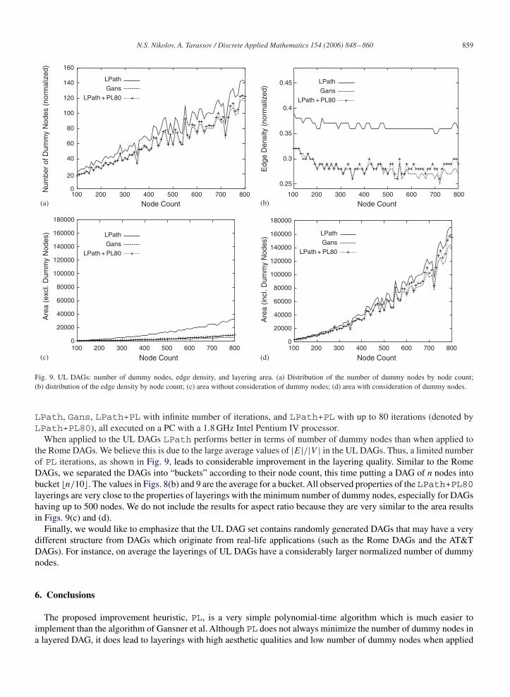
LPath, Gans, LPath+PL with infinite number of iterations, and LPath+PL with up to 80 iterations (denoted byLPath+PL80), all executed on a PC with a 1.8 GHz Intel Pentium IV processor.

When applied to the UL DAGs LPath performs better in terms of number of dummy nodes than when applied tothe Rome DAGs. We believe this is due to the large average values of |E|/|V | in the UL DAGs. Thus, a limited numberof PL iterations, as shown in Fig. 9, leads to considerable improvement in the layering quality. Similar to the RomeDAGs, we separated the DAGs into “buckets” according to their node count, this time putting a DAG of n nodes intobucket �n/10�. The values in Figs. 8(b) and 9 are the average for a bucket. All observed properties of the LPath+PL80layerings are very close to the properties of layerings with the minimum number of dummy nodes, especially for DAGshaving up to 500 nodes. We do not include the results for aspect ratio because they are very similar to the area resultsin Figs. 9(c) and (d).

Finally, we would like to emphasize that the UL DAG set contains randomly generated DAGs that may have a verydifferent structure from DAGs which originate from real-life applications (such as the Rome DAGs and the AT&TDAGs). For instance, on average the layerings of UL DAGs have a considerably larger normalized number of dummynodes.

6. Conclusions

The proposed improvement heuristic, PL, is a very simple polynomial-time algorithm which is much easier toimplement than the algorithm of Gansner et al. Although PL does not always minimize the number of dummy nodes ina layered DAG, it does lead to layerings with high aesthetic qualities and low number of dummy nodes when applied


after the longest-path layering algorithm. The worst-case time complexity of PL is O(|D(G,L)| ∗ |V | ∗ (|E| + |V |))where |D(G,L)| is the number of dummy nodes in a layering L of a DAG G. Although slower than the algorithm ofGansner et al., the longest-path algorithm followed by PL performs fast enough when applied to DAGs with up to 100nodes taken from practical applications (the Rome and the AT&T graph sets).

As a further step, it might be fruitful to adopt some of the more recent static scheduling algorithms for DAG layeringand to experiment with applying PL for improving the quality of their output. Also, it would be interesting to study theimpact of an improvement technique as PL from the static scheduling point of view.

References

[1] J. Branke, S. Leppert, M. Middendorf, P. Eades, Width-restriced layering of acyclic digraphs with consideration of dummy nodes, Inform.Process. Lett. 81 (2) (2002) 59–63.

[2] M.J. Carpano, Automatic display of hierarchized graphs for computer aided decision analysis, IEEE Trans. Systems Man Cybernet. 10 (11)(1980) 705–715.

[3] E.G. Coffman, R.L. Graham, Optimal scheduling for two processor systems, Acta Inform. 1 (1972) 200–213.[4] G. Di Battista, A. Garg, G. Liotta, R. Tamassia, E. Tassinari, F. Vargiu, An experimental comparison of four graph drawing algorithms, Comput.

Geometry: Theory Appl. 7 (1997) 303–316.[5] P. Eades, K. Sugiyama, How to draw a directed graph, J. Inform. Process. 13 (4) (1990) 424–437.[6] A. Frick, Upper bounds on the number of hidden nodes in Sugiyama’s algorithm, in: S. North (Ed.), Graph Drawing: Proceedings of the

Symposium on Graph Drawing, GD ’96, Lecture Notes in Computer Science, vol. 1190, Springer, Berlin, 1997, pp. 169–183.[7] E.R. Gansner, E. Koutsofios, S.C. North, K.-P. Vo, A technique for drawing directed graphs, IEEE Trans. Software Engrg. 19 (3) (1993)

214–230.[8] P. Healy, N.S. Nikolov, A branch-and-cut approach to the directed acyclic graph layering problem, in: M. Goodrich, S. Koburov (Eds.), Graph

Drawing: Proceedings of 10th International Symposium, GD 2002, Lecture Notes in Computer Science, vol. 2528, Springer, Berlin, 2002, pp.98–109.

[9] P. Healy, N.S. Nikolov, How to layer a directed acyclic graph, in: P. Mutzel, M. Jünger, S. Leipert (Eds.), Graph Drawing: Proceedings of NinthInternational Symposium, GD 2001, Lecture Notes in Computer Science, vol. 2265, Springer, Berlin, 2002, pp. 16–30.

[10] T. Hu, Parallel sequencing and assembly line problems, Oper. Res. 9 (1961) 841–848.[11] Y.-K. Kwok, I. Ahmad, Static scheduling algorithms for allocating directed task graphs to multiprocessors, ACM Comput. Surveys 31 (4) (1999)

406–471.[12] I. Lemke, Entwicklung und Implementierung eines Visualisierungswerkzeuges für Anwendungen im Übersetzerbau, Diplomarbeit, Universität

des Saarlandes, FB 14 Informatik, 1994.[13] K. Mehlhorn, S. Näher, C. Uhrig, The LEDA platform of combinatorial and geometric computing, in: Automata, Languages and Programming,

1997, pp. 7–16.[14] G.L. Nemhauser, L.A. Wolsey, Integer and Combinatorial Optimization, Wiley-Interscience Series in Discrete Mathematics and Optimization,

Wiley, New York, 1988.[15] K. Sugiyama, K. Misue, Graph drawing by the magneting spring model, J. Visual Languages Comput. 6 (3) (1995) 217–231.[16] K. Sugiyama, S. Tagawa, M. Toda, Methods for visual understanding of hierarchical system structures, IEEE Trans. Systems Man Cybernet.

11 (2) (1981) 109–125.[17] J. Ulman, NP-complete scheduling problems, J. Comput. System Sci. 10 (1975) 384–393.[18] J. Utech, J. Branke, H. Schmeck, P. Eades, An evolutionary algorithm for drawing directed graphs, in: Proceedings of the 1998 International

Conference on Imaging Science, Systems, and Technology (CISST’98), 1998, pp. 154–160.[19] J.N. Warfield, Crossing theory and hierarchy mapping, IEEE Trans. Systems Man Cybernet. 7 (7) (1977) 502–523.

Documents

Graph layering by promotion of nodes