Graphical Analysis and Fitting

Physics 3110Dr. Rebecca Forrest

University of Houston

The Art of Experimental Physics, D. Preston & E. Dietz, NY, John Wiley, (1991), pp. 18 - 22

Plotting on the Computer

• Excel• Gnuplot – http://www.gnuplot.info/• PSI plot• Mathcad• Mathmatica• Origin• SciDavis• Etc.

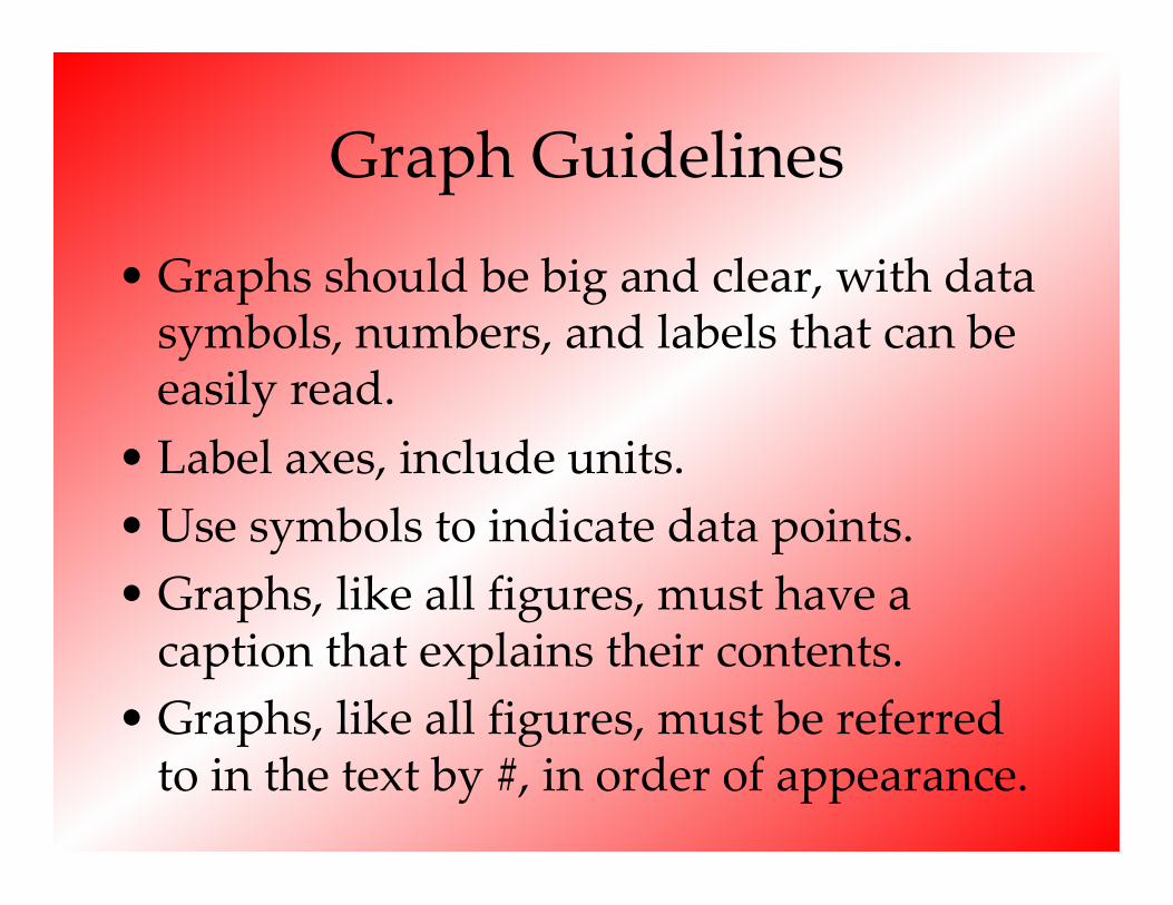
Graph Guidelines

• Graphs should be big and clear, with data symbols, numbers, and labels that can be easily read.

• Label axes, include units.• Use symbols to indicate data points.• Graphs, like all figures, must have a

caption that explains their contents. • Graphs, like all figures, must be referred

to in the text by #, in order of appearance.

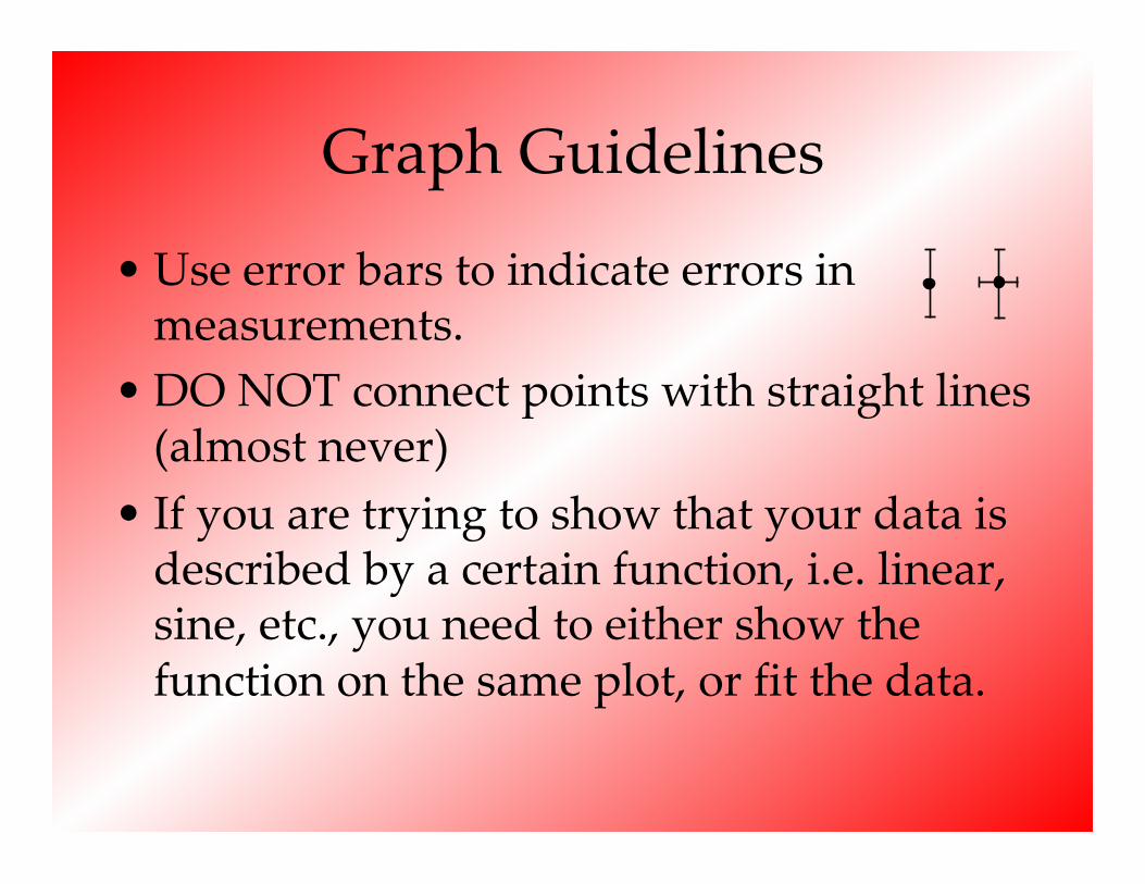
Graph Guidelines

• Use error bars to indicate errors in measurements.

• DO NOT connect points with straight lines (almost never)

• If you are trying to show that your data is described by a certain function, i.e. linear, sine, etc., you need to either show the function on the same plot, or fit the data.

Graphs in Your Reports

“Locality of Quark-Hadron Duality and Deviations from Quark Counting Rules Above the Resonance Region”, Qiang Zhao1 and Frank E. Close,Phys. Rev. Lett., 022004, 91, 2003.

“…Taking account of the nondegeneracy for n < 2 gives the solid curve in Fig. 1, which includes prominent well known resonances. Including nondegeneracy for n < 4 [26] gives the dotted curve in Fig. 1.”

Examples

Good • Caption • Fig. 1 is mentioned by name in text above.

Bad • All fonts too small • No error bars • Too much info in Caption.

Good • Caption • Axes are labeled and units are shown • Legend

Bad • No data symbols shown • Instead, data points connected with lines

Good • Caption • Fig. 1 is mentioned by name in text above. • Axes are labeled • Data symbols shown with error bars

Bad • All fonts too small • Axis units not labeled • This is an exception about connecting data points. Without it, the data trend is not obvious. • Meter reading vs. distance

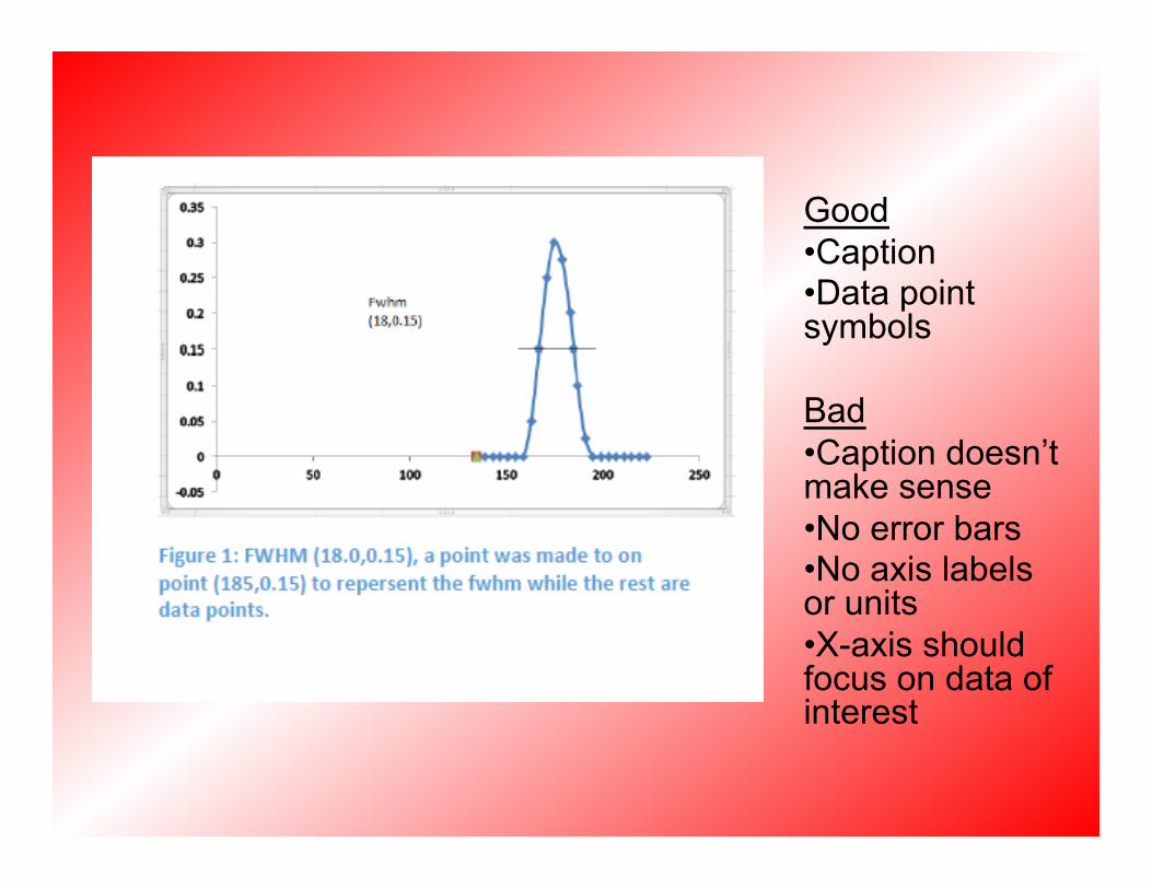
Good • Caption • Data point symbols

Bad • Caption doesn’t make sense • No error bars • No axis labels or units • X-axis should focus on data of interest

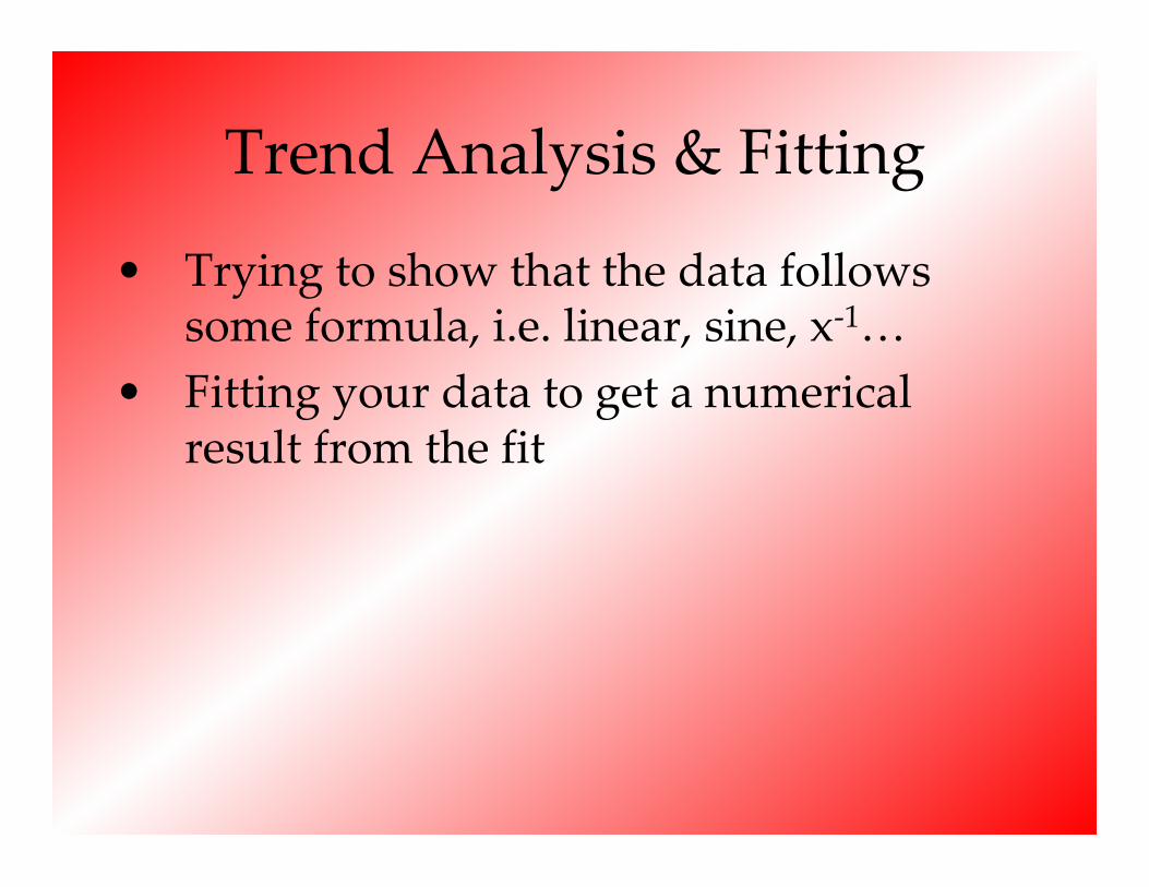
Trend Analysis & Fitting

•  Trying to show that the data follows some formula, i.e. linear, sine, x-1…

•  Fitting your data to get a numerical result from the fit

Trend Analysis

0

10

20

30

40

50

60

0 20 40 60 80 100

Inte

nsity

(Am

ps)

angle (degrees)

-10

0

10

20

30

40

50

60

70

0 20 40 60 80 100

Inte

nsity

(Am

ps)

angle (degrees)

peak

sin^2 theta

sin theta

Data Fitting •  A set of observations/data are given •  You want to fit a “model” function to the data •  Figure-of-merit function measures agreement

between the data and the model

• w Data • -- Fit 1, y = a1 x2 + a2 x + a3

• -- Fit 2, y = a1 x3 + a2 x2 + a3 x + a4

y = 0.2203x2 + 1.7072x - 8.6522R² = 0.98583

y = -0.0245x3 + 0.9557x2 - 4.3281x + 2.6731R² = 0.99411

-20

0

20

40

60

80

100

120

140

0 5 10 15 20 25

acce

lera

tion

(cm

/s^2

)

position (cm)

• y(xi; a1 …am)

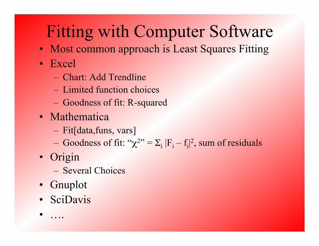
Fitting with Computer Software •  Most common approach is Least Squares Fitting •  Excel

–  Chart: Add Trendline –  Limited function choices –  Goodness of fit: R-squared

•  Mathematica –  Fit[data,funs, vars] –  Goodness of fit: “χ2” = Σi |Fi – fi|2, sum of residuals

•  Origin –  Several Choices

•  Gnuplot •  SciDavis •  ….

Least Squares Fitting

Adapted from:

Numerical Recipes The Art of Scientific Computing W.H. Press, S.A. Teukolsky, W.T.

Vetterling, B.P. Flannery Cambridge University Press 1992 New (and free Older versions) at

www.nr.com

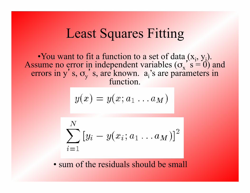
Least Squares Fitting • You want to fit a function to a set of data (xi, yi).

Assume no error in independent variables (σx’s = 0) and errors in y’s, σy’s, are known. ai’s are parameters in

function.

•  sum of the residuals should be small

Central Limit Theorem

•  For large enough N, the measurement errors follow a Gaussian distribution with standard deviations σ

•  Minimize χ2:

Minimize χ2

( ) 02

=∂χ∂

ia Solve

• To apply this, we need to know the function y(xi; a1…am)

Example: Least Squares Fitting to a Straight Line •  Also called linear regression

•  Minimize χ2: ( ) 02

=∂χ∂

ia Solve

Taking Derivatives

= -2(Sy – aS – bSx)

= -2(Sxy – aSx – bSxx)

Solution to Linear System

• Now you have a & b that give the best fit to your data. What are the errors in a & b?

Propagation of Errors Errors in a & b

• Variances in the Estimates

€

δw2 = ∂w∂xiδxi( )2

i∑ ,

Goodness of Fit •  Sum of residuals

–  should be close to 0 •  χ2

–  should be small, χ2 ~ ν, where ν = degrees of freedom = number of data points minus the number of parameters being fit

•  Reduced χ2 = χ2 /ν –  χ2/ν ~ 1.0 is good

•  Others …

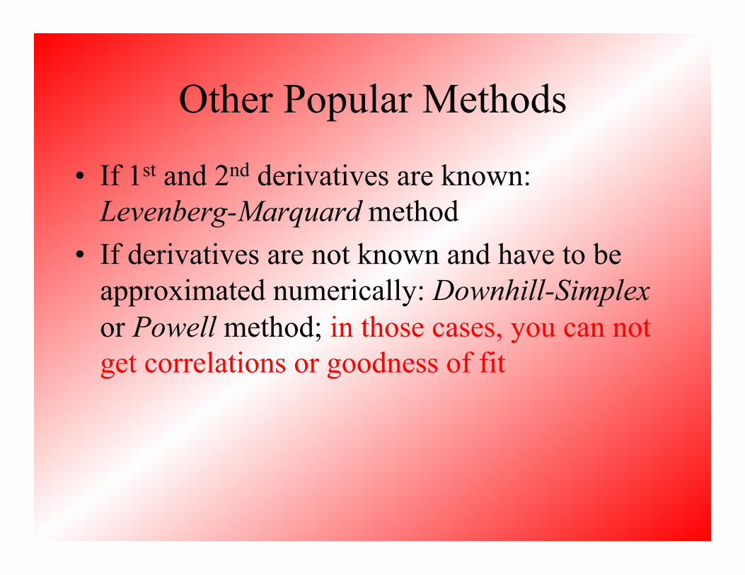
Other Popular Methods

•  If 1st and 2nd derivatives are known: Levenberg-Marquard method

•  If derivatives are not known and have to be approximated numerically: Downhill-Simplex or Powell method; in those cases, you can not get correlations or goodness of fit

Using Gnuplot for Fitting

•  http://www.gnuplot.info/ •  Gnuplot is a portable command-line driven

interactive data and function plotting utility for UNIX, IBM OS/2, MS Windows, DOS, Macintosh, VMS, Atari and many other platforms. The software is copyrighted but freely distributed .

•  For MS Windows, download the file with win32 in its name.

•  Gnuplot’s fit uses the nonlinear least-squares Marquardt-Levenberg algorithm

Windows GUI

File/Demos

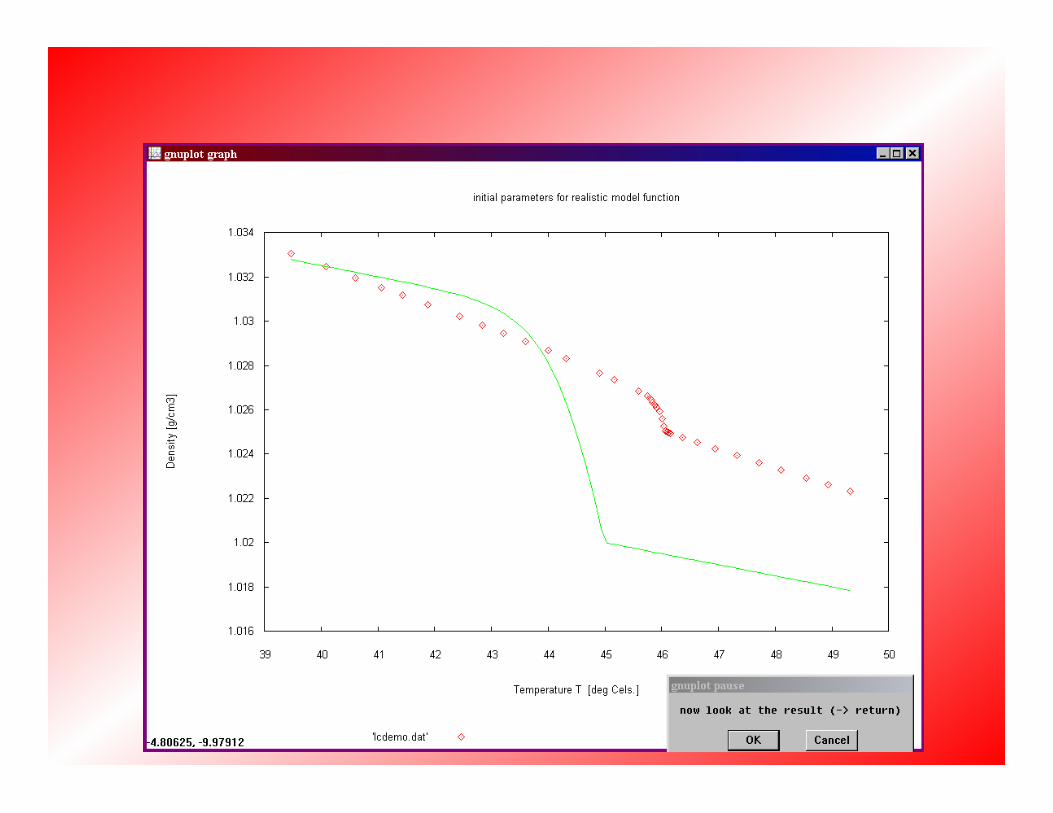
Fit Demo for Density data • Plot ‘lcdemo.dat’

Unweighted Linear Fit

• Fit l(x) ‘lcdemo.dat via y0, m • Plot ‘lcdemo.dat’, l(x)

• fit l(x) 'lcdemo.dat' using 1:2:3 via y0, m

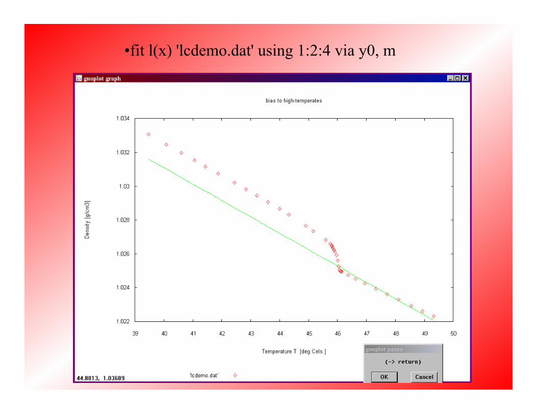
• fit l(x) 'lcdemo.dat' using 1:2:4 via y0, m

• plot 'lcdemo.dat' using 1:2:5 with errorbars

Final Parameters and Error

Homework 1.  (3 pts.) Plot the data in data.dat with error bars, found on Blackboard, using

a computer program. The 3rd column is the error. The plot should have the appropriate format, but no caption is required.

2.  (7 pts.) Fit the data in data.dat to this Gaussian distribution,

•  In computer syntax, this could be written as N(x) = (A/(sqrt(2*3.1416)*w)) * exp(-(x-xave)**2/(2*(w**2)))

•  Show a plot of the data with error bars and the fit, and report the fitted values of A, σ, and xave. The plot should have the appropriate format, but no caption is required. (This may count as the plot for part 1.)

•  If available, report the errors in A, σ, and xave, and an estimate of the goodness of the fit, i.e. reduced χ2 or R2.

•  Tell me what program you used.

N(x) = A2πσ

e−(x−x )2

2σ 2