Graphical Modelling in Geneticsand Systems Biology

Marco Scutari

m.scutari@ucl.ac.ukGenetics Institute

University College London

October 30th, 2012

Marco Scutari University College London

Current Practices in Bayesian

Networks Modelling

Marco Scutari University College London

Current Practices in Bayesian Networks Modelling

Bayesian Networks Modelling Framework

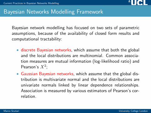
Bayesian network modelling has focused on two sets of parametricassumptions, because of the availability of closed form results andcomputational tractability:

• discrete Bayesian networks, which assume that both the globaland the local distributions are multinomial. Common associa-tion measures are mutual information (log-likelihood ratio) andPearson’s X2;

• Gaussian Bayesian networks, which assume that the global dis-tribution is multivariate normal and the local distributions areunivariate normals linked by linear dependence relationships.Association is measured by various estimators of Pearson’s cor-relation.

Marco Scutari University College London

Current Practices in Bayesian Networks Modelling

Open Problems

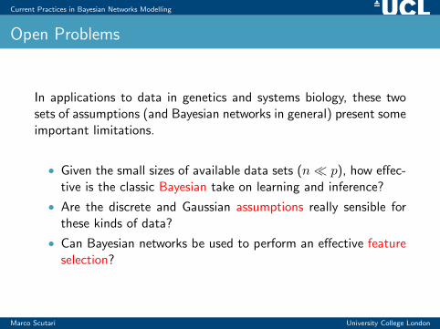
In applications to data in genetics and systems biology, these twosets of assumptions (and Bayesian networks in general) present someimportant limitations.

• Given the small sizes of available data sets (n� p), how effec-tive is the classic Bayesian take on learning and inference?

• Are the discrete and Gaussian assumptions really sensible forthese kinds of data?

• Can Bayesian networks be used to perform an effective featureselection?

Marco Scutari University College London

Data in Genetics and Systems

Biology

Marco Scutari University College London

Data in Genetics and Systems Biology

Overview

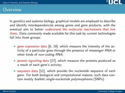
In genetics and systems biology, graphical models are employed to describeand identify interdependencies among genes and gene products, with theeventual aim to better understand the molecular mechanisms that linkthem. Data commonly made available for this task by current technologiesfall into three groups:

• gene expression data [6, 19], which measure the intensity of the ac-tivity of a particular gene through the presence of messenger RNA orother kinds of non-coding RNA;

• protein signalling data [17], which measure the proteins produced asa result of each gene’s activity;

• sequence data [11], which provide the nucleotide sequence of eachgene. For both biological and computational reasons, such data con-tain mostly biallelic single-nucleotide polymorphisms (SNPs).

Marco Scutari University College London

Data in Genetics and Systems Biology

Gene Expression Data

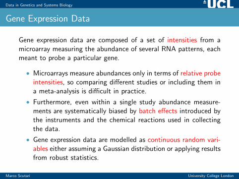
Gene expression data are composed of a set of intensities from amicroarray measuring the abundance of several RNA patterns, eachmeant to probe a particular gene.

• Microarrays measure abundances only in terms of relative probeintensities, so comparing different studies or including them ina meta-analysis is difficult in practice.

• Furthermore, even within a single study abundance measure-ments are systematically biased by batch effects introduced bythe instruments and the chemical reactions used in collectingthe data.

• Gene expression data are modelled as continuous random vari-ables either assuming a Gaussian distribution or applying resultsfrom robust statistics.

Marco Scutari University College London

Data in Genetics and Systems Biology

Gene Expression Data

Gat1

Uga3

Dal80

Asp3

Tat1

Opt2

Gap1Nit1

Met13

Arg80

His5Agp5

Tat2

Dal7Dal2

Dal3

Bap1

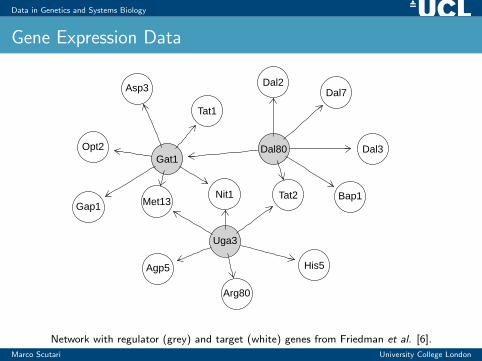
Network with regulator (grey) and target (white) genes from Friedman et al. [6].

Marco Scutari University College London

Data in Genetics and Systems Biology

Models for Gene Expression Data

Two classes of undirected graphical models are in common use:

• relevance networks [2], also known in statistics as correlationgraphs, which are constructed using marginal dependencies.

• gene association networks, also known as concentration graphsor graphical Gaussian models [24], which consider conditionalrather than marginal dependencies.

Bayesian network use by Friedman et al. [7], and has also beenreviewed more recently in Friedman [4]. Inference procedures areusually unable to identify a single best BN, settling instead on a setof equally well behaved models. For this reason, it is important toincorporate prior biological knowledge into the network through theuse of informative priors [12].

Marco Scutari University College London

Data in Genetics and Systems Biology

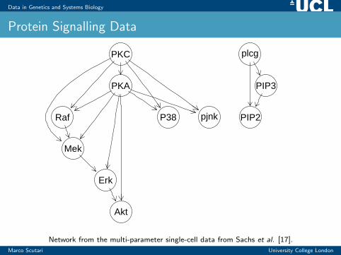
Protein Signalling Data

Protein signalling data are similar to gene expression data in manyrespects.

• In fact, they are often used to investigate indirectly the expres-sion of a set of genes.

• The relationships between proteins are indicative of their phys-ical location within the cell and of the development over timeof the molecular processes (pathways) they are involved in.

• Protein signalling data sometimes have sample sizes that aremuch larger than either gene expression or sequence data.

Marco Scutari University College London

Data in Genetics and Systems Biology

Protein Signalling Data

Akt

Erk

Mek

P38 PIP2

PIP3

pjnk

PKA

PKC plcg

Raf

Network from the multi-parameter single-cell data from Sachs et al. [17].

Marco Scutari University College London

Data in Genetics and Systems Biology

Sequence Data

Sequence data analysis focuses on modelling the behaviour of oneor more phenotypic traits (e.g. the presence of a disease in humans,yield in plants, milk production in cows) by capturing direct andindirect causal genetic effects:

• the identification of the genes that are strongly associated witha trait is called a genome-wide association study (GWAS);

• the prediction of a trait for the purpose of implementing aselection program (i.e. to decide which plants or animals tocross so that the offspring exhibit) is called genomic selection(GS).

Marco Scutari University College London

Data in Genetics and Systems Biology

Models for Sequence Data

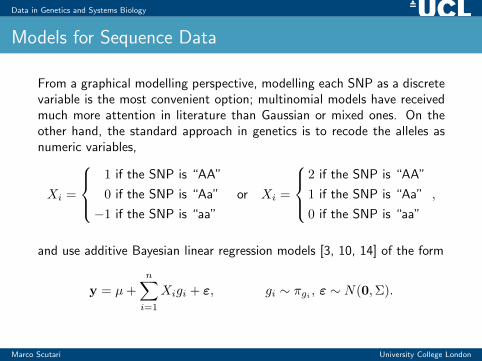
From a graphical modelling perspective, modelling each SNP as a discretevariable is the most convenient option; multinomial models have receivedmuch more attention in literature than Gaussian or mixed ones. On theother hand, the standard approach in genetics is to recode the alleles asnumeric variables,

Xi =

1 if the SNP is “AA”

0 if the SNP is “Aa”

−1 if the SNP is “aa”

or Xi =

2 if the SNP is “AA”

1 if the SNP is “Aa”

0 if the SNP is “aa”

,

and use additive Bayesian linear regression models [3, 10, 14] of the form

y = µ+

n∑i=1

Xigi + ε, gi ∼ πgi , ε ∼ N(0,Σ).

Marco Scutari University College London

Bayesian Statistics

Marco Scutari University College London

Bayesian Statistics

Bayesian Basics: Priors and Posteriors

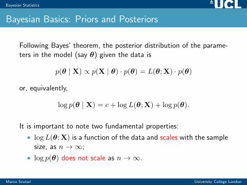
Following Bayes’ theorem, the posterior distribution of the parame-ters in the model (say θ) given the data is

p(θ | X) ∝ p(X | θ) · p(θ) = L(θ;X) · p(θ)

or, equivalently,

log p(θ | X) = c+ logL(θ;X) + log p(θ).

It is important to note two fundamental properties:

• logL(θ;X) is a function of the data and scales with the samplesize, as n→∞;

• log p(θ) does not scale as n→∞.

Marco Scutari University College London

Bayesian Statistics

Posteriors in “Small n, Large p” Settings

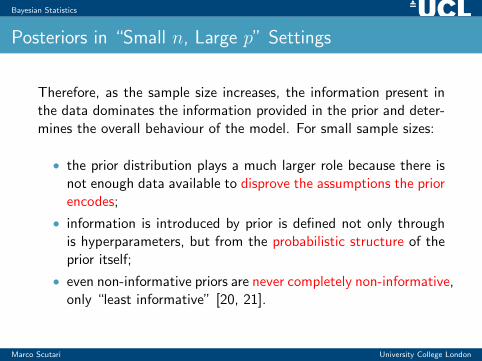
Therefore, as the sample size increases, the information present inthe data dominates the information provided in the prior and deter-mines the overall behaviour of the model. For small sample sizes:

• the prior distribution plays a much larger role because there isnot enough data available to disprove the assumptions the priorencodes;

• information is introduced by prior is defined not only throughis hyperparameters, but from the probabilistic structure of theprior itself;

• even non-informative priors are never completely non-informative,only “least informative” [20, 21].

Marco Scutari University College London

Bayesian Statistics

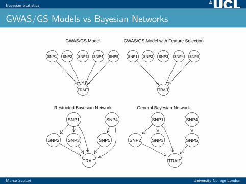
GWAS/GS Models vs Bayesian Networks

GWAS/GS Model

SNP1 SNP2 SNP3 SNP4 SNP5

TRAIT

GWAS/GS Model with Feature Selection

SNP1 SNP2 SNP3 SNP4 SNP5

TRAIT

Restricted Bayesian Network

SNP1

SNP2 SNP3

SNP4

SNP5

TRAIT

General Bayesian Network

SNP1

SNP2 SNP3

SNP4

SNP5

TRAIT

Marco Scutari University College London

Parametric Assumptions

Marco Scutari University College London

Parametric Assumptions

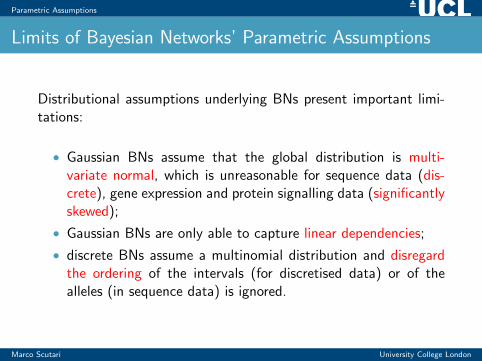
Limits of Bayesian Networks’ Parametric Assumptions

Distributional assumptions underlying BNs present important limi-tations:

• Gaussian BNs assume that the global distribution is multi-variate normal, which is unreasonable for sequence data (dis-crete), gene expression and protein signalling data (significantlyskewed);

• Gaussian BNs are only able to capture linear dependencies;

• discrete BNs assume a multinomial distribution and disregardthe ordering of the intervals (for discretised data) or of thealleles (in sequence data) is ignored.

Marco Scutari University College London

Parametric Assumptions

Limits of Bayesian Networks’ Parametric Assumptions

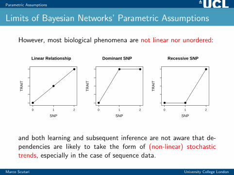
However, most biological phenomena are not linear nor unordered:

Linear Relationship

SNP

TR

AIT

0 1 2

●

●

●

Dominant SNP

SNP

TR

AIT

0 1 2

●

● ●

Recessive SNP

SNP

TR

AIT

0 1 2

● ●

●

and both learning and subsequent inference are not aware that de-pendencies are likely to take the form of (non-linear) stochastictrends, especially in the case of sequence data.

Marco Scutari University College London

Parametric Assumptions

A Test for Trend

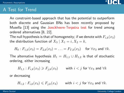
An constraint-based approach that has the potential to outperformboth discrete and Gaussian BNs has been recently proposed byMusella [13] using the Jonckheere-Terpstra test for trend amongordered alternatives [8, 22].The null hypothesis is that of homogeneity; if we denote with Fi,k(x3)the distribution function of X3 | X1 = i,X2 = k,

H0 : F1,k(x3) = F2,k(x3) = . . . = FT,k(x3) for ∀x3 and ∀k.

The alternative hypothesis H1 = H1,1 ∪ H1,2 is that of stochasticordering, either increasing

H1,1 : Fi,k(x3) > Fj,k(x3) with i < j for ∀x3 and ∀k

or decreasing

H1,2 : Fi,k(x3) 6 Fj,k(x3) with i < j for ∀x3 and ∀k.

Marco Scutari University College London

Parametric Assumptions

The Jonckheere-Terpstra Test Statistic

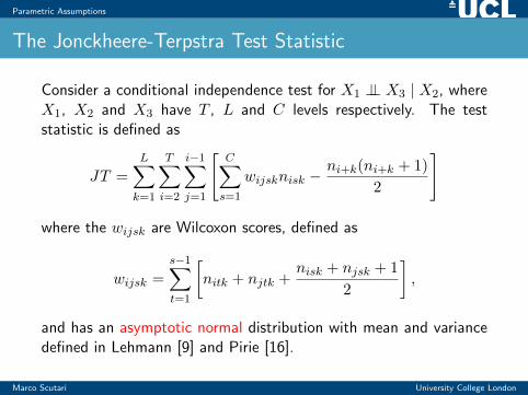
Consider a conditional independence test for X1 ⊥⊥ X3 | X2, whereX1, X2 and X3 have T , L and C levels respectively. The teststatistic is defined as

JT =

L∑k=1

T∑i=2

i−1∑j=1

[C∑

s=1

wijsknisk −ni+k(ni+k + 1)

2

]

where the wijsk are Wilcoxon scores, defined as

wijsk =

s−1∑t=1

[nitk + njtk +

nisk + njsk + 1

2

],

and has an asymptotic normal distribution with mean and variancedefined in Lehmann [9] and Pirie [16].

Marco Scutari University College London

Feature Selection

Marco Scutari University College London

Feature Selection

Feature Selection in Genetics and Systems Biology

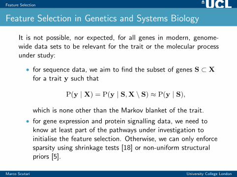
It is not possible, nor expected, for all genes in modern, genome-wide data sets to be relevant for the trait or the molecular processunder study:

• for sequence data, we aim to find the subset of genes S ⊂ Xfor a trait y such that

P(y | X) = P(y | S,X \ S) ≈ P(y | S),

which is none other than the Markov blanket of the trait.

• for gene expression and protein signalling data, we need toknow at least part of the pathways under investigation toinitialise the feature selection. Otherwise, we can only enforcesparsity using shrinkage tests [18] or non-uniform structuralpriors [5].

Marco Scutari University College London

Feature Selection

Markov Blankets for GWAS/GS Models

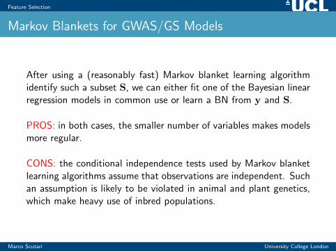
After using a (reasonably fast) Markov blanket learning algorithmidentify such a subset S, we can either fit one of the Bayesian linearregression models in common use or learn a BN from y and S.

PROS: in both cases, the smaller number of variables makes modelsmore regular.

CONS: the conditional independence tests used by Markov blanketlearning algorithms assume that observations are independent. Suchan assumption is likely to be violated in animal and plant genetics,which make heavy use of inbred populations.

Marco Scutari University College London

Feature Selection

Markov Blankets for Gene Expression Data

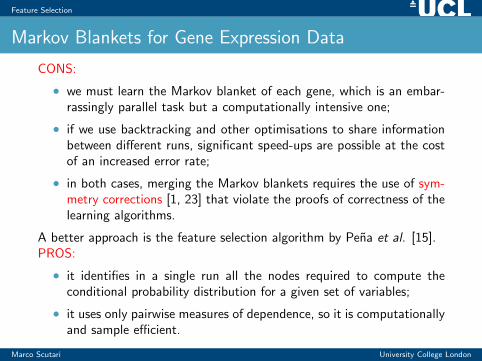
CONS:

• we must learn the Markov blanket of each gene, which is an embar-rassingly parallel task but a computationally intensive one;

• if we use backtracking and other optimisations to share informationbetween different runs, significant speed-ups are possible at the costof an increased error rate;

• in both cases, merging the Markov blankets requires the use of sym-metry corrections [1, 23] that violate the proofs of correctness of thelearning algorithms.

A better approach is the feature selection algorithm by Pena et al. [15].PROS:

• it identifies in a single run all the nodes required to compute theconditional probability distribution for a given set of variables;

• it uses only pairwise measures of dependence, so it is computationallyand sample efficient.

Marco Scutari University College London

Thanks!

Marco Scutari University College London

References

Marco Scutari University College London

References

References I

C. F. Aliferis, A. Statnikov, I. Tsamardinos, S. Mani, and X. D. Koutsoukos.Local Causal and Markov Blanket Induction for Causal Discovery and FeatureSelection for Classification Part I: Algorithms and Empirical Evaluation.Journal of Machine Learning Research, 11:171–234, 2010.

A. J. Butte, P. Tamayo, D. Slonim, T. R. Golub, and I. S. Kohane.Discovering Functional Relationships Between RNA Expression andChemotherapeutic Susceptibility Using Relevance Networks.PNAS, 97:12182–12186, 2000.

R. L Fernando D. Habier, K. Kizilkaya, and D. J. Garrick.Extension of the Bayesian Alphabet for Genomic Selection.BMC Bioinformatics, 12(186):1–12, 2011.

N. Friedman.Inferring Cellular Networks Using Probabilistic Graphical Models.Science, 303:799–805, 2004.

N. Friedman and D. Koller.Being Bayesian about Bayesian Network Structure: A Bayesian Approach toStructure Discovery in Bayesian Networks.Machine Learning, 50(1–2):95–126, 2003.

Marco Scutari University College London

References

References II

N. Friedman, M. Linial, and I. Nachman.Using Bayesian Networks to Analyze Expression Data.Journal of Computational Biology, 7:601–620, 2000.

N. Friedman, M. Linial, I. Nachman, and D. Pe’er.Using Bayesian Networks to Analyze Gene Expression Data.Journal of Computational Biology, 7:601–620, 2000.

A. Jonckheere.A Distribution-Free k-Sample Test Against Ordered Alternatives.Biometrika, 41:133–145, 1954.

E. L. Lehmann.Nonparametrics: Statistical Methods Based on Ranks.Springer, 2006.

T. H. E. Meuwissen, B. J. Hayes, and M. E. Goddard.Prediction of Total Genetic Value Using Genome-Wide Dense Marker Maps.Genetics, 157:1819–1829, 2001.

Marco Scutari University College London

References

References III

G. Morota, B. D. Valente, G. J. M. Rosa, K. A. Weigel, and D. Gianola.An Assessment of Linkage Disequilibrium in Holstein Cattle Using a BayesianNetwork.Journal of Animal Breeding and Genetics, 2012.In print.

S. Mukherjee and T. P. Speed.Network Inference using Informative Priors.PNAS, 105:14313–14318, 2008.

F. Musella.Learning a Bayesian Network from Ordinal Data.Working Paper 139, Dipartimento di Economia, Universita degli Studi “RomaTre”, 2011.

T. Park and G. Casella.The Bayesian Lasso.Journal of the American Statistical Association, 103(482), 2008.

Marco Scutari University College London

References

References IV

J. Pena, R. Nilsson, J. Bjorkegren, and J. Tegner.Identifying the Relevant Nodes Without Learning the Model.In Proceedings of the 22nd Conference Annual Conference on Uncertainty inArtificial Intelligence (UAI-06), pages 367–374, 2006.

W. Pirie.Jonckheere Tests for Ordered Alternatives.In Encyclopaedia of Statistical Sciences, pages 315–318. Wiley, 1983.

K. Sachs, O. Perez, D. Pe’er, D. A. Lauffenburger, and G. P. Nolan.Causal Protein-Signaling Networks Derived from Multiparameter Single-CellData.Science, 308(5721):523–529, 2005.

M. Scutari and A. Brogini.Bayesian Network Structure Learning with Permutation Tests.Communications in Statistics – Theory and Methods, 41(16–17):3233–3243,2012.

P. Spirtes, C. Glymour, and R. Scheines.Causation, Prediction, and Search.MIT Press, 2000.

Marco Scutari University College London

References

References V

H. Steck.Learning the Bayesian Network Structure: Dirichlet Prior versus Data.In Proceedings of the 24th Conference Annual Conference on Uncertainty inArtificial Intelligence (UAI-08), pages 511–518, 2008.

H. Steck and T. Jaakkola.On the Dirichlet Prior and Bayesian Regularization.In Advances in Neural Information Processing Systems (NIPS), pages 697–704,2002.

T. J. Terpstra.The Asymptotic Normality and Consistency of Kendall’s Test Against TrendWhen the Ties Are Present in One Ranking.Indagationes Mathematicae, 14:327–333, 1952.

I. Tsamardinos, L. E. Brown, and C. F. Aliferis.The Max-Min Hill-Climbing Bayesian Network Structure Learning Algorithm.Machine Learning, 65(1):31–78, 2006.

J. Whittaker.Graphical Models in Applied Multivariate Statistics.Wiley, 1990.

Marco Scutari University College London