Embed Size (px)
Citation preview
Graphical models for combining multiple data sources
Nicky BestSylvia Richardson
Chris Jackson
Imperial College BIAS node
with thanks to Peter Green
Outline
• Overview of graphical modelling• Case study 1: Water disinfection byproducts and
adverse birth outcomes – Modelling multiple sources of bias in observational
studies
• Case study 2: Socioeconomic factors and limiting long term illness– Combining individual and aggregate level data– Simulation study – Application to Census and Health Survey for England

Graphical modelling
Modelling
Inference
Mathematics
Algorithms

1. Mathematics
Modelling
Inference
Mathematics
Algorithms
• Key idea: conditional independence• X and Y are conditionally independent given Z if, knowing
Z, discovering Y tells you nothing more about XP(X | Y, Z) = P(X | Z)

Example: Mendelian inheritance
• Z = genotype of parents • X, Y = genotypes of 2 children• If we know the genotype of the parents, then the
children’s genotypes are conditionally independent
Z
X Y

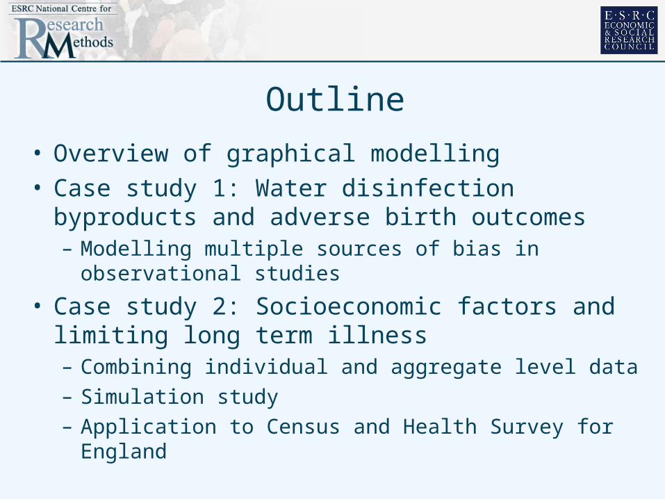
Joint distributions and graphical models
Use ideas from graph theory to: • represent structure of a joint probability
distribution…..• …..by encoding conditional independencies
• Factorization thm:
Jt distribution P(V) = P(v | parents[v])
D
EB
CA
F

Where does the graph come from?
• Genetics– pedigree (family tree)
• Physical, biological, social systems– supposed causal effects
• Contingency tables– hypothesis tests on data
• Gaussian case– non-zeros in inverse covariance matrix
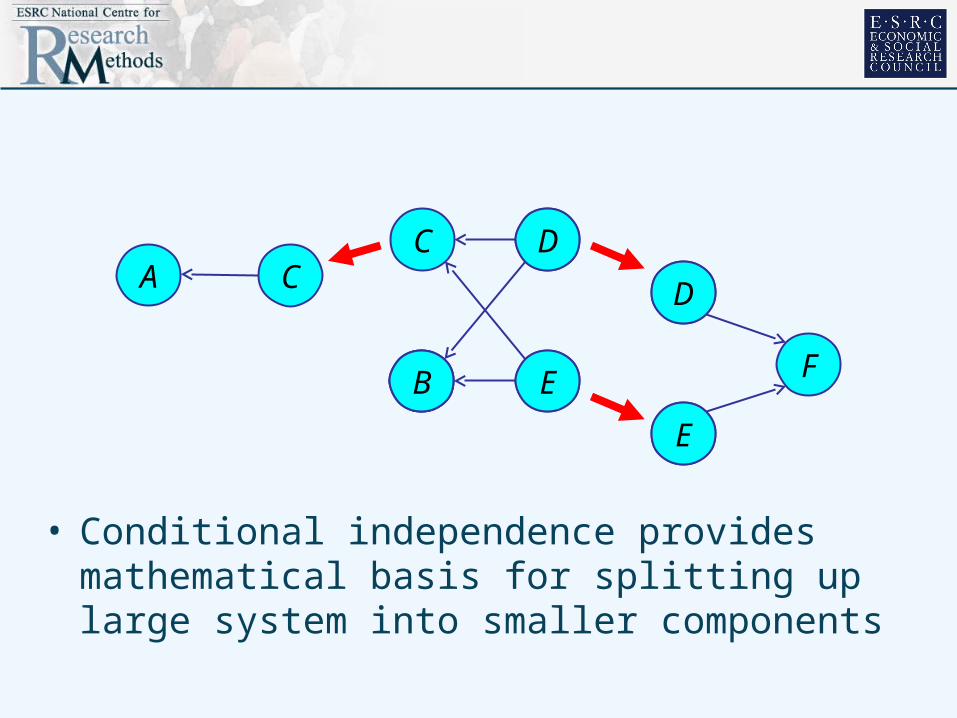
• Conditional independence provides mathematical basis for splitting up large system into smaller components
D
EB
CA
F
• Conditional independence provides mathematical basis for splitting up large system into smaller components
D
EB
C
D
E
F
CA
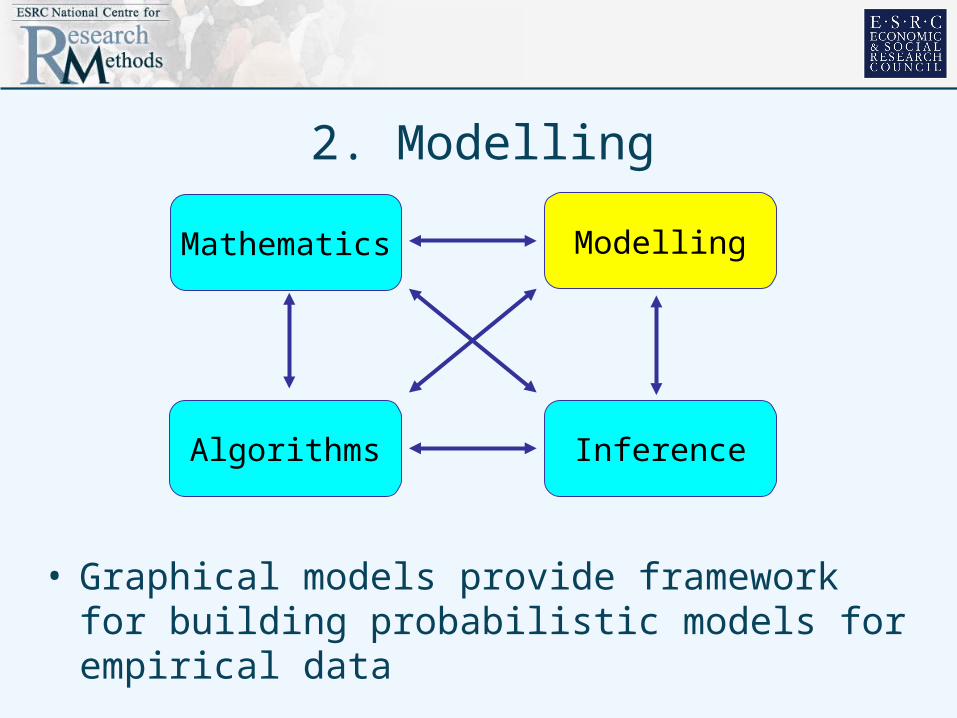
2. Modelling
• Graphical models provide framework for building probabilistic models for empirical data
Modelling
Inference
Mathematics
Algorithms
Building complex models
Key idea• understand complex system• through global model• built from small pieces
– comprehensible– each with only a few variables– modular
Example: Case study 1
• Epidemiological study of birth defects and mothers’ exposure to water disinfection byproducts
• Background– Chlorine added to tap water supply for disinfection– Reacts with natural organic matter in water to form
unwanted byproducts (including trihalomethanes, THMs)– Some evidence of adverse health effects (cancer, birth
defects) associated with exposure to high levels of THM– We are carrying out study in Great Britain using routine
data, to investigate risk of birth defects associated with exposure to different THM levels

Data sources
• National postcoded births register• National and local congenital anomalies registers• Routinely monitored THM concentrations in tap
water samples for each water supply zone within 14 different water company regions
• Census data – area level socioeconomic factors• Millenium cohort study (MCS) – individual level
outcomes and confounder data on sample of mothers
• Literature relating to factors affecting personal exposure (uptake factors, water consumption, etc.)
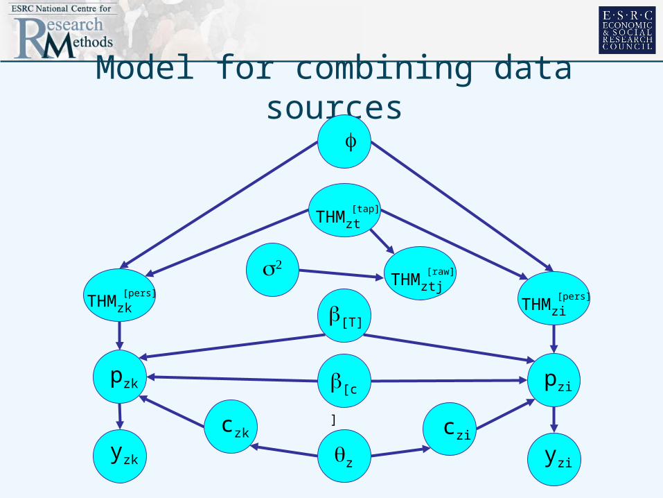
Model for combining data sources
yzk
[c]
[T]
pzk
yzi
pzi
czk
z
czi
THMzk[pers]
THMzt[tap]
THMztj[raw]
THMzi[pers]

Model for combining data sources
yzk
[c]
[T]
pzk
yzi
pzi
czk
z
czi
THMzk[pers]
THMzt[tap]
THMztj[raw]
THMzi[pers]
Regression model for national data relating risk of
birth defects (pzk) to mother’s THM exposure
and other confounders (czk)

Model for combining data sources
yzk
[c]
[T]
pzk
yzi
pzi
czk
z
czi
THMzk[pers]
THMzt[tap]
THMztj[raw]
THMzi[pers]
Regression model for MCS data relating risk of birth defects (pzi) to mother’s
THM exposure and other confounders (czi)

Model for combining data sources
yzk
[c]
[T]
pzk
yzi
pzi
czk
z
czi
THMzk[pers]
THMzt[tap]
THMztj[raw]
THMzi[pers]
Missing data model to estimate confounders (czk)
for mothers in national data, using information on within area distribution of
confounders in MCS
Model for combining data sources
yzk
[c]
[T]
pzk
yzi
pzi
czk
z
czi
THMzk[pers]
THMzt[tap]
THMztj[raw]
THMzi[pers]
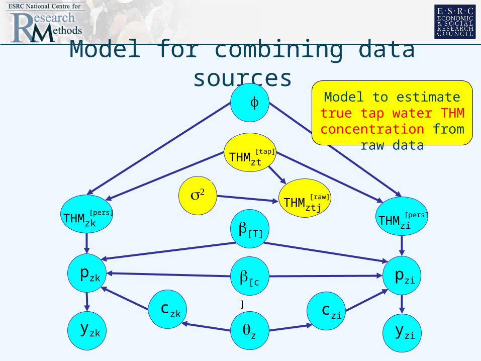
Model to estimate true tap water THM concentration
from raw data
Model for combining data sources
yzk
[c]
[T]
pzk
yzi
pzi
czk
z
czi
THMzk[pers]
THMzt[tap]
THMztj[raw]
THMzi[pers]
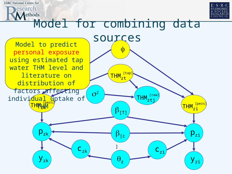
Model to predict personal exposure using estimated tap water THM level and
literature on distribution of factors affecting individual
uptake of THM

3. Inference
Modelling
Inference
Mathematics
Algorithms

Bayesian

… or non Bayesian

Bayesian Full Probability Modelling
• Graphical approach to building complex models lends itself naturally to Bayesian inferential process
• Graph defines joint probability distribution on all the ‘nodes’ in the model
• Condition on parts of graph that are observed (data)
• Update probabilities of remaining nodes using Bayes theorem
• Automatically propagates all sources of uncertainty

4. Algorithms
• Many algorithms, including MCMC, are able to exploit graphical structure
• MCMC: subgroups of variables updated randomly• Ensemble converges to equilibrium (e.g. posterior) dist.
Modelling
Inference
Mathematics
Algorithms
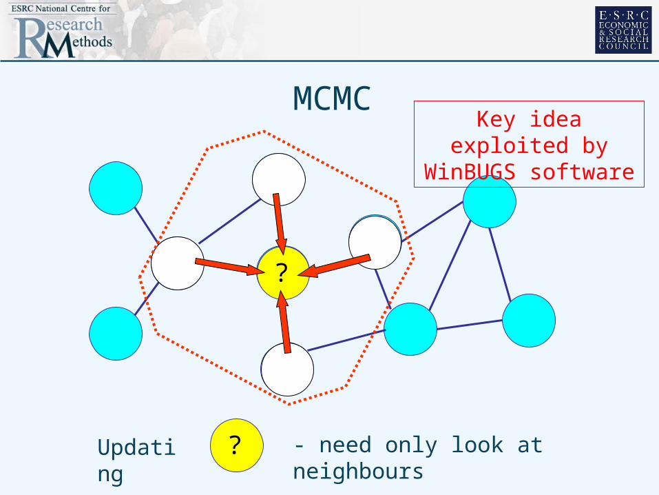
MCMC
?
?Updating - need only look at neighbours
Key idea exploited by WinBUGS software
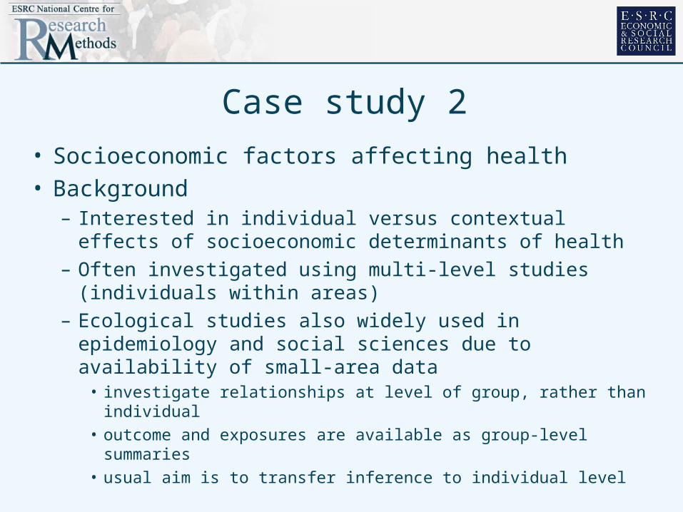
Case study 2
• Socioeconomic factors affecting health• Background
– Interested in individual versus contextual effects of socioeconomic determinants of health
– Often investigated using multi-level studies (individuals within areas)
– Ecological studies also widely used in epidemiology and social sciences due to availability of small-area data
• investigate relationships at level of group, rather than individual• outcome and exposures are available as group-level summaries• usual aim is to transfer inference to individual level
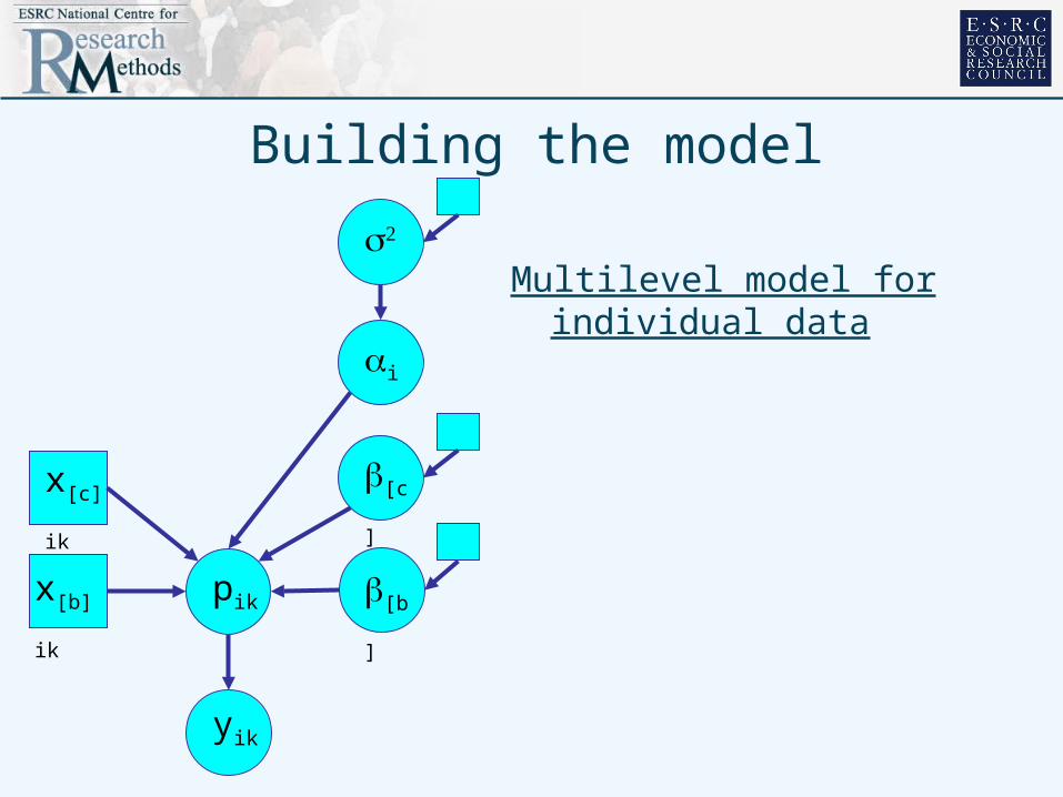
Building the model
x[c]ik
yik
[b]
[c]
i
pikx[b]ik
Multilevel model for individual data

Building the model
Multilevel model for individual data
yik ~ Bernoulli(pik), person k, area i
x[c]ik
yik
[b]
[c]
i
pikx[b]ik
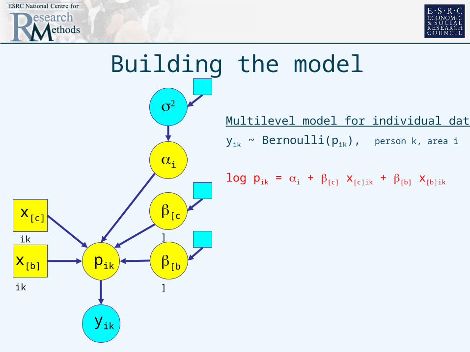
Building the model
Multilevel model for individual data
yik ~ Bernoulli(pik), person k, area i
x[c]ik
yik
[b]
[c]
i
pikx[b]ik
log pik = i + [c] x[c]ik + [b] x[b]ik

Building the model
Multilevel model for individual data
yik ~ Bernoulli(pik), person k, area i
x[c]ik
yik
[b]
[c]
i
pikx[b]ik
log pik = i + [c] x[c]ik + [b] x[b]ik
i ~ Normal(0, )

Building the model
Multilevel model for individual data
yik ~ Bernoulli(pik), person k, area i
x[c]ik
yik
[b]
[c]
i
pikx[b]ik
log pik = i + [c] x[c]ik + [b] x[b]ik
i ~ Normal(0, )
Prior distributions on 2, [c], [b]
Building the model
X[c]i
Yi
[b]
[c]
i
i X[b]i
V[c]i
Ni
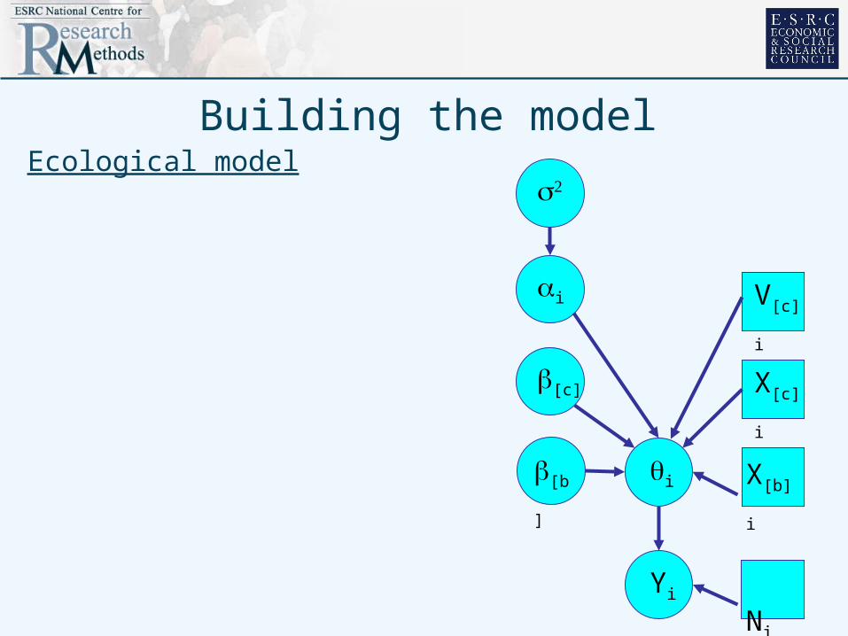
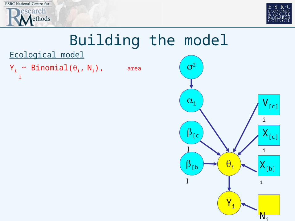
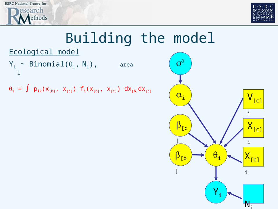
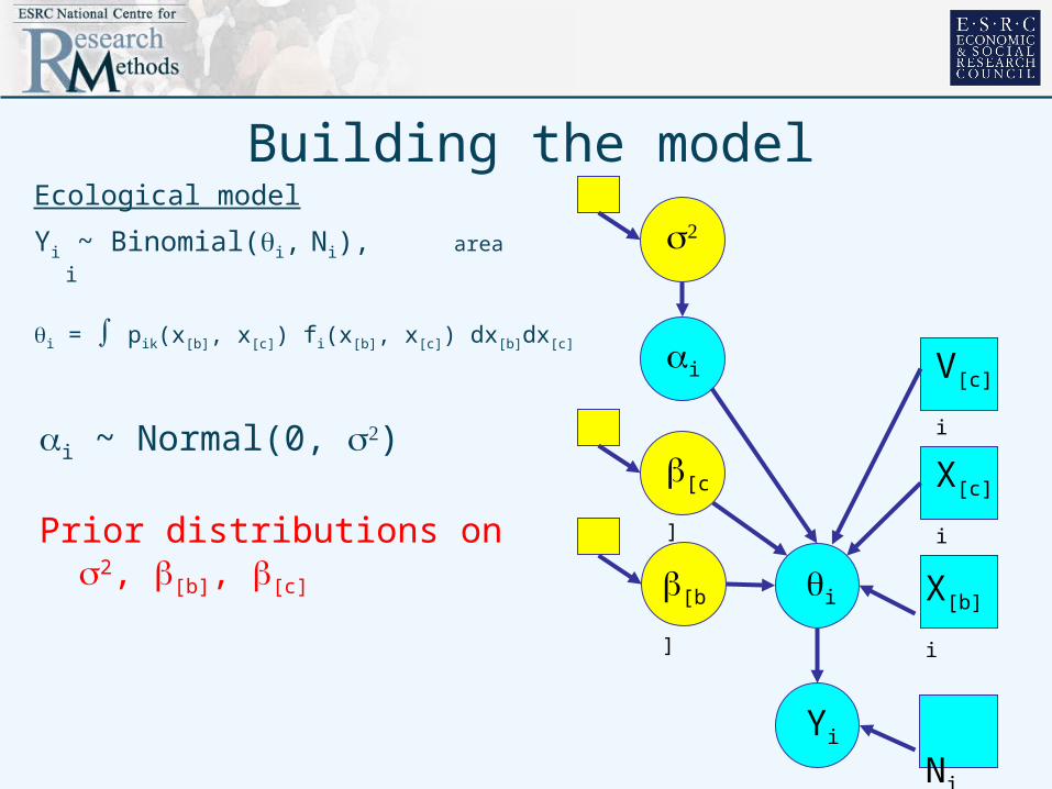
Ecological model
Building the model
X[c]i
Yi
[b]
[c]
i
i X[b]i
V[c]i
Ecological model
Yi ~ Binomial(i, Ni), area i
Ni
Building the model
X[c]i
Yi
[b]
i
i X[b]i
V[c]i
Ecological model
Yi ~ Binomial(i, Ni), area i
i = pik(x[b], x[c]) fi(x[b], x[c]) dx[b]dx[c]
Ni
[c]
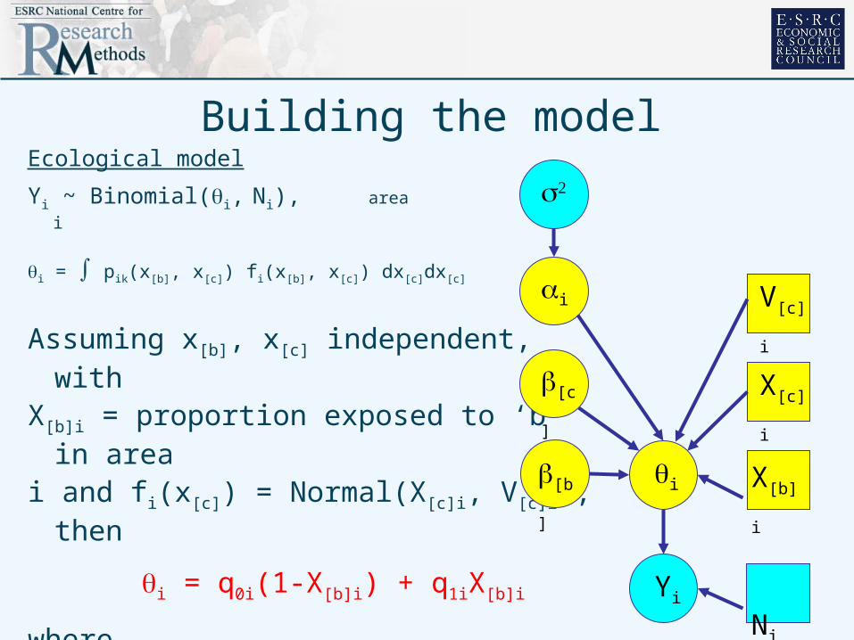
Assuming x[b], x[c] independent, with
X[b]i = proportion exposed to ‘b’ in area
i and fi(x[c]) = Normal(X[c]i, V[c]i), then
i = q0i(1-X[b]i) + q1iX[b]i
where
q0i = marginal prob of disease for unexposed
= exp(i + [c]X[c]I + 2[c]V[c]i/2)
Building the model
X[c]i
Yi
[b]
i
i X[b]i
V[c]i
Ecological model
Yi ~ Binomial(i, Ni), area i
i = pik(x[b], x[c]) fi(x[b], x[c]) dx[c]dx[c]
Ni
[c]

Assuming x[b], x[c] independent, with
X[b]i = proportion exposed to ‘b’ in area
i and fi(x[c]) = Normal(X[c]i, V[c]i), then
i = q0i(1-X[b]i) + q1iX[b]i
where
q1i = marginal prob of disease for exposed
= exp(i + [b] + [c]X[c]I + 2[c]V[c]i/2)
Building the model
X[c]i
Yi
[b]
i
i X[b]i
V[c]i
Ecological model
Yi ~ Binomial(i, Ni), area i
i = pik(x[b], x[c]) fi(x[b], x[c]) dx[b]dx[c]
Ni
[c]

Building the model
X[c]i
Yi
[b]
[c]
i
i X[b]i
V[c]i
Ecological model
Yi ~ Binomial(i, Ni), area i
i = pik(x[b], x[c]) fi(x[b], x[c]) dx[b]dx[c]
Ni
i ~ Normal(0, )
Building the model
X[c]i
Yi
[b]
[c]
i
i X[b]i
V[c]i
Ecological model
Yi ~ Binomial(i, Ni), area i
i = pik(x[b], x[c]) fi(x[b], x[c]) dx[b]dx[c]
Ni
i ~ Normal(0, )
Prior distributions on 2, [b], [c]

Combining individual and aggregate data
• Individual level survey data often lack power to inform about contextual and/or individual-level effects
• Even when correct (integrated) model used, ecological data often contain little information about some or all effects of interest
• Can we improve inference by combining both types of model / data?

Combining individual and aggregate data
X[c]i
Yi
[b]
[c]
i
i X[b]i
V[c]i
Ni
x[c]ik
yik
[b]
[c]
i
pikx[b]ik
Multilevel model for individual data
Ecological model
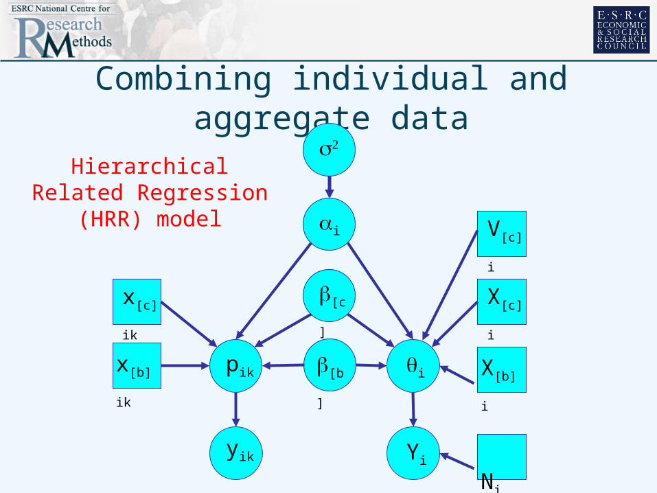
Combining individual and aggregate data
X[c]i
Yi
[b]
[c]
i
i X[b]i
V[c]i
Ni
x[c]ik
yik
pikx[b]ik
Hierarchical Related Regression (HRR) model
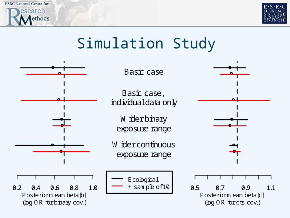
Simulation Study
Posterior mean beta[b](log OR for binary cov.)
0.2 0.4 0.6 0.8 1.00.2 0.4 0.6 0.8 1.0Ecological+ sample of 10
Wider continuousexposure range
Wider binaryexposure range
Basic case,individual data only
Basic case
Posterior mean beta[c](log OR for cts cov.)
0.5 0.7 0.9 1.10.5 0.7 0.9 1.1
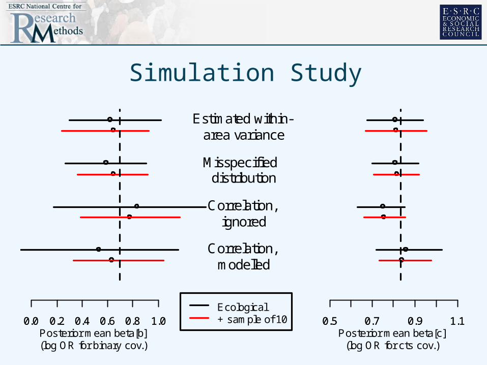
Simulation Study
Posterior mean beta[b](log OR for binary cov.)
0.0 0.2 0.4 0.6 0.8 1.00.0 0.2 0.4 0.6 0.8 1.0Ecological+ sample of 10
Correlation,modelled
Correlation,ignored
Misspecified distribution
Estimated within-area variance
Posterior mean beta[c](log OR for cts cov.)
0.5 0.7 0.9 1.10.5 0.7 0.9 1.1

Simulation Study
Posterior mean beta[b](log OR for binary cov.)
0.0 0.2 0.4 0.6 0.8 1.00.0 0.2 0.4 0.6 0.8 1.0Ecological+ sample of 10
Large ME, individualdata only
Large measurementerror
Small measurementerror
Posterior mean beta[c](log OR for cts cov.)
0.0 0.2 0.4 0.6 0.8 1.00.0 0.2 0.4 0.6 0.8 1.0

Comments
• Inference from aggregate data can be unbiased provided exposure contrasts between areas are high (and appropriate integrated model used)
• Combining aggregate data with small samples of individual data can reduce bias when exposure contrasts are low
• Combining individual and aggregate data can reduce MSE of estimated compared to individual data alone
• Individual data cannot help if individual-level model is misspecified

Application to LLTI
• Health outcome– Limiting Long Term Illness (LLTI) in men aged 40-59 yrs
living in London
• Exposures– ethnicity (white/non-white), income, area deprivation
• Data sources– Aggregate: 1991 Census aggregated to ward level – Individual: Health Survey for England (with ward identifier)
• 1-9 observations per ward (median 1.6)

Ward level data
Deprivation
Deprivation
Dep
rivat
ion
% non white
% non white% non white
Mean income
Mea
n in
com
e
Mea
n in
com
e
Pre
vale
nce
of
LLT
I
Pre
vale
nce
of
LLT
I
Pre
vale
nce
of
LLT
I
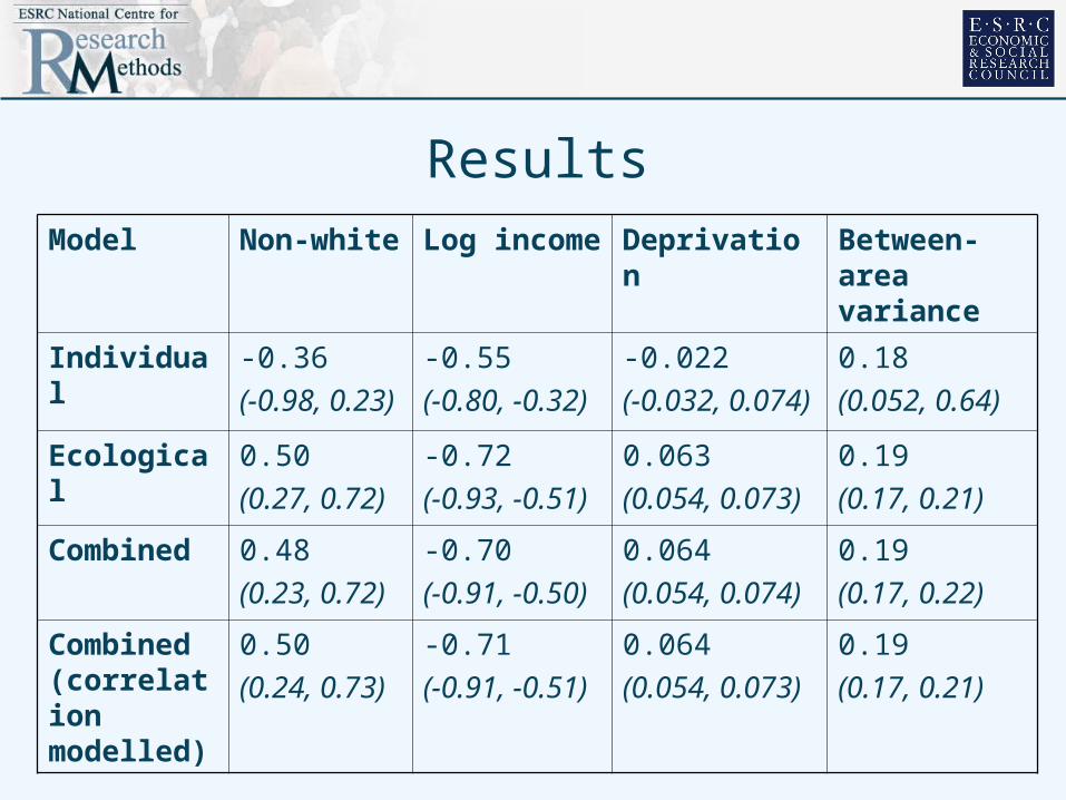
ResultsModel Non-white Log income Deprivation Between-
area variance
Individual -0.36
(-0.98, 0.23)
-0.55
(-0.80, -0.32)
-0.022
(-0.032, 0.074)
0.18
(0.052, 0.64)
Ecological 0.50
(0.27, 0.72)
-0.72
(-0.93, -0.51)
0.063
(0.054, 0.073)
0.19
(0.17, 0.21)
Combined 0.48
(0.23, 0.72)
-0.70
(-0.91, -0.50)
0.064
(0.054, 0.074)
0.19
(0.17, 0.22)
Combined (correlation modelled)
0.50
(0.24, 0.73)
-0.71
(-0.91, -0.51)
0.064
(0.054, 0.073)
0.19
(0.17, 0.21)

Concluding Remarks
• Graphical models are powerful and flexible tool for building realistic statistical models for complex problems– Applicable in many domains– Allow exploiting of subject matter knowledge– Allow formal combining of multiple data sources– Built on rigorous mathematics– Principled inferential methods
Thank you for your attention!