Embed Size (px)
Citation preview

Graphical Real-time Simulation Tool for Passive
UHF RFID Environments
by
Jonathan E. Wolk
Submitted to the Department of Electrical Engineering and ComputerScience
in partial fulfillment of the requirements for the degree of
Master of Engineering in Electrical Engineering and Computer Science
at the
MASSACHUSETTS INSTITUTE OF TECHNOLOGY
June 2005
@ Massachusetts Institute of Technology 2005. All rights reserved.
MASSACHUSETTS INSTr1'TEOF TECHNOLOGY
JUL 18 2005Author ........ ..... LI. RAR1Ej j
Depar --- c,-6 11 7ad Ceiuputurm orie ce
May 19, 2005
Certified by. ............l W. Engels
Research ScientistcmL:- 0 ervisor
Accepted by .... ..
i-unu k,. SmithChairman, Department Committee on Graduate Students
BARKER

2

Graphical Real-time Simulation Tool for Passive UHF RFID
Environments
by
Jonathan E. Wolk
Submitted to the Department of Electrical Engineering and Computer Scienceon May 19, 2005, in partial fulfillment of the
requirements for the degree ofMaster of Engineering in Electrical Engineering and Computer Science
Abstract
In this thesis, I present the design and implementation of a real-time simulation tool,RFID Vis, that is used to simulate a UHF RFID environment. The simulation toolsimulates environments containing to pallets of cases as is common in parts of thesupply chain. The simulation tool consists of two parts, a graphical front end whichinterfaces with the user as well as displayes the electromagnetic power present ina given volume of space in an intuitive manner and an electromagnetics simulationengine which takes care of all the electromagnetic calculations and approximations.The simulation tool is written in C++ using Microsoft DirectX 9.0 to interface withthe graphics hardware. RFID Vis enables users to quickly simulate a real worldoperating scenario providing insights and building intuition.
Thesis Supervisor: Daniel W. EngelsTitle: Research Scientist
3

4

Acknowledgments
I first want to thank my mother, Magdalena, for having the patience to raise me
and for sticking through my graduate career without too much complaining. I also
want to thank my father and grandparents for helping me through both the MIT
undergraduate and graduate years. Dr. Daniel Engels and Dr. Rich Fletcher, thank
you for allowing me such creative freedom and guidance when tackling this project.
Lastly, I want to thank all of the brothers at Pi Lambda Phi fraternity, Massachusetts
Theta chapter, for lifting me up when I was down and making these years more fun
and more bearable.
5

6

Contents
1 Introduction 15
1.1 Introduction . . . . . . . . . . . . . . . . . . . . . . . . . . . . . . . . 15
1.2 Introduction to Passive RFID . . . . . . . . . . . . . . . . . . . . . . 17
1.3 Motivation for a Simulator . . . . . . . . . . . . . . . . . . . . . . . . 18
1.4 Description of Simulator . . . . . . . . . . . . . . . . . . . . . . . . . 19
1.5 Thesis Summary . . . . . . . . . . . . . . . . . . . . . . . . . . . . . 21
2 The Intuitive Graphical User Interface 25
2.1 User Interfaces and Their Challenges . . . . . . . . . . . . . . . . . . 25
2.2 Previous Work on Volumetric Data . . . . . . . . . . . . . . . . . . . 27
2.2.1 Voxel Based Direct Volume Rendering . . . . . . . . . . . . . 28
2.2.2 Surface Based Volume Rendering . . . . . . . . . . . . . . . . 29
2.3 I-GUI Design and Goals . . . . . . . . . . . . . . . . . . . . . . . . . 30
2.3.1 I-GUI Extensibility . . . . . . . . . . . . . . . . . . . . . . . . 30
2.3.2 I-GUI User Interaction . . . . . . . . . . . . . . . . . . . . . . 31
3 I-GUI Architecture and Implementation 35
3.1 Environment Renderable Classes . . . . . . . . . . . . . . . . . . . . 35
3.1.1 Renderable Class . . . . . . . . . . . . . . . . . . . . . . . . . 36
3.1.2 Geometry Class . . . . . . . . . . . . . . . . . . . . . . . . . . 37
3.2 Physical Objects . . . . . . . . . . . . . . . . . . . . . . . . . . . . . 37
3.2.1 PhysicalObject . . . . . . . . . . . . . . . . . . . . . . . . . . 38
3.2.2 Reflector Class . . . . . . . . . . . . . . . . . . . . . . . . . . 41
7

3.2.3 Antenna Class . . . . . . . . . . . . . . . . . . .
3.2.4 Rendering Antenna Power . . . . . . . . . . . .
3.2.5 MaterialBox Class . . . . . . . . . . . . . . . .
3.2.6 Tag Class . . . . . . . . . . . . . . . . . . . . .
3.3 Environment Management Classes . . . . . . . . . . . .
3.3.1 SceneManager Class . . . . . . . . . . . . . . .
3.3.2 Other Environment Management Classes . . . .
4 Analysis of the I-GUI
4.1 I-G UI Usability . . . . . . . . . . . . . . . . . . . . . .
4.2 Analysis of Electromagnetic Power Rendering . . . . .
4.2.1 Texture Slices . . . . . . . . . . . . . . . . . . .
4.2.2 Texturing Methods . . . . . . . . . . . . . . . .
4.2.3 Summary of Electromagnetic Power Rendering .
5 The
5.1
5.2
5.3
5.4
Simulation Engine
Introduction to Electromagnetics Engines
Previous Work on E&M Algorithms . . . . .
5.2.1 Exact Numerical Methods . . . . . .
5.2.2 Approximate Numerical Methods . .
Challenges with Real-Time . . . . . . . . . .
Simulation Engine Goals and Design . . . .
5.4.1 Calculation of Electromagnetic Fields
5.4.2 Engine Design . . . . . . . . . . . . .
6 Simulation Engine Architecture and Implementation
6.1 Engine Components . . . . . . . . . . . . . . . . . . . .
6.1.1 SceneManager Class . . . . . . . . . . . . . . .
6.1.2 EMEngine Class . . . . . . . . . . . . . . . . .
6.1.3 RunSimulationDialog Class . . . . . . . . . . .
6.1.4 EMAlgorithm Class . . . . . . . . . . . . . . . .
8
41
42
45
45
46
46
47
49
. . . . . . . . 49
. . . . . . . . 52
. . . . . . . . 52
. . . . . . . . 55
. . . . . . . . 58
59
59
60
60
61
62
63
63
64
67
67
68
68
69
70

6.2 Ray Tracing Algorithm Components . . . . . . . . . . . . . . . . . .
6.2.1 ElectricRay Class . . . . . . . . . . . . . . . . . . . . . . . . .
6.2.2 EMRayTracing Algorithm . . . . . . . . . . . . . . . . . . . .
7 Analysis of the Simulation Engine
7.1 Analysis of EMRayTracing Algorithm . . . . . . . . . . . . . . . . . .
7.1.1 Single Ray Complexity . . . . . . . . . . . . . . . . . . . . . .
7.1.2 Initial Ray Complexity . . . . . . . . . . . . . . . . . . . . . .
7.1.3 Resolution Complexity . . . . . . . . . . . . . . . . . . . . . .
7.1.4 Real-time Analysis . . . . . . . . . . . . . . . . . . . . . . . .
7.1.5 Analysis of Produced Results . . . . . . . . . . . . . . . . . .
7.1.6 Summary of EMRayTracing Analysis . . . . . . . . . . . . . .
8 Conclusions
8.1 RFID Vis Conclusions
8.2 Future Work . . . . . . . .
A User Manual for Simulation Tool
A.1 Installation ... .............
A.2 Camera Movement ...........
A.3 Coordinate System . . . . . . . . .
A .4 O bjects . . . . . . . . . . . . . . .
A.4.1 Antenna Object . . . . . . .
A.4.2 MaterialBox Object . . . . .
A.4.3 Tag Object . . . . . . . . .
A.5 Clicking and Dragging . . . . . . .
A.6 Running a Simulation . . . . . . . .
A.6.1 Real-time Simulations . . .
A.6.2 More Accurate Simulations .
9
70
71
74
83
83
84
85
88
90
94
98
101
101
103
107
107
107
108
109
109
110
111
111
112
112
113
. . . . . . . . . . . . . . . . . . . . . . . .
. . . . . . . . . . . . . . . . . . . . . . . .

10

List of Figures
2-1 Example Voxel Grid . . . . . . . . . . . . . . . . . . . . . . . . . . . 28
3-1 Example Properties Dialog . . . . . . . . . . . . . . . . . . . . . . . . 40
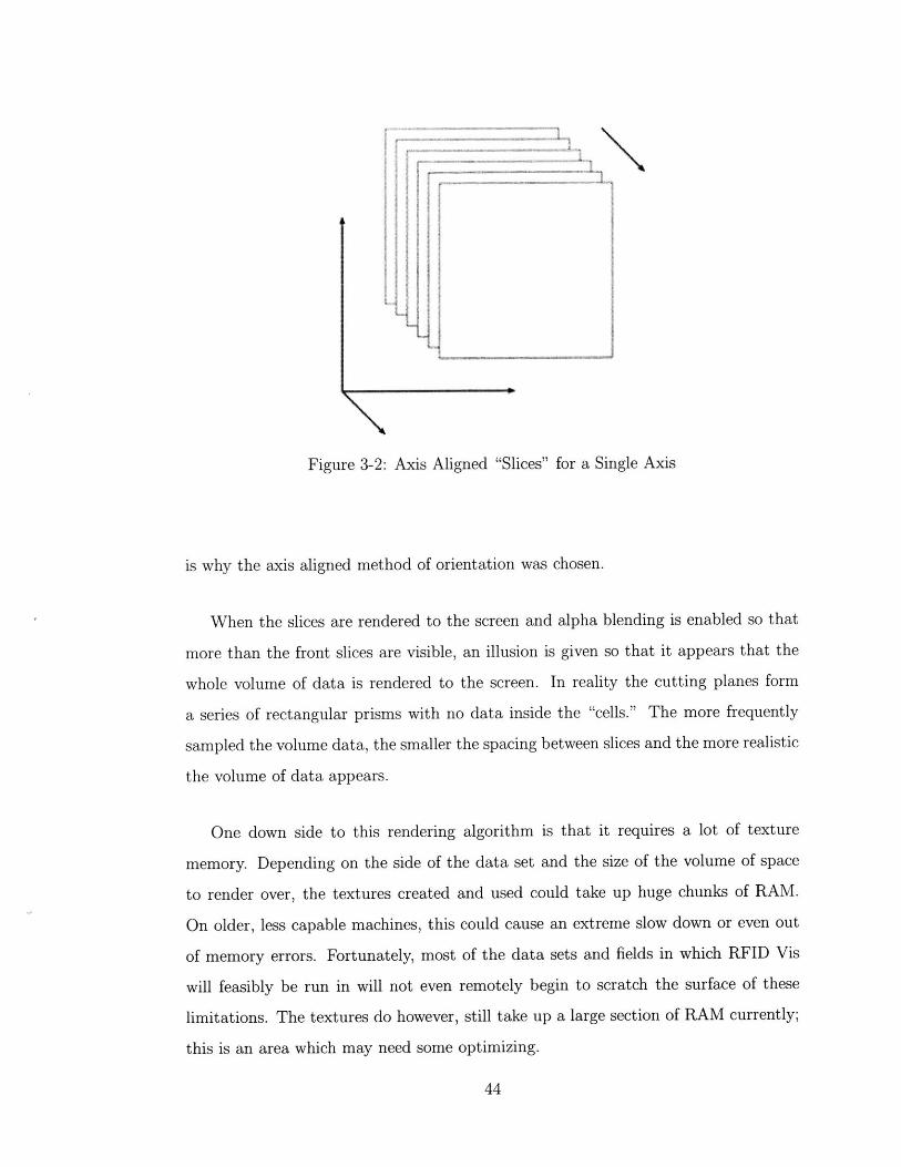
3-2 Axis Aligned "Slices" for a Single Axis . . . . . . . . . . . . . . . . . 44
3-3 A Tag object that is "off" and "on" . . . . . . . . . . . . . . . . . . . 45
4-1 Graph of Rendering Times for Different Numbers of Slices . . . . . . 54
4-2 Electromagnetic Power Rendering with 8 Slices per Axis . . . . . . . 55
4-3 Electromagnetic Power Rendering with 32 Slices per Axis . . . . . . . 56
4-4 Electromagnetic Power Rendering with 24 Slices per Axis . . . . . . . 56
6-1 Incident Wave Reflecting Off of Reflector Surface . . . . . . . . . . . 77
6-2 Incident Wave Transmitting Through Reflector Surface . . . . . . . . 79
7-1 Example of a Complex RFID Environment . . . . . . . . . . . . . . . 86
7-2 Simulation Time Depedence on Maximum Recursion Depth . . . . . . 87
7-3 Graph of Simulation Times Based on a Single Pattern Dimension . . 91
7-4 Graph of Simulation Times Based on Simulation Resolution . . . . . 92
7-5 Simulated Destructive Interference . . . . . . . . . . . . . . . . . . . 97
7-6 Simulated Electromagnetic Power Propagating Through Water . . . . 99
11

12

List of Tables
4.1 Effects of the Number of Slices on Rendering Times . . . . . . . . . . 54
4.2 Effects of the Texturing Method on Rendering Times . . . . . . . . . 58
7.1 Effects of the Antenna Pattern Dimension on Simulation Times . . . 89
7.2 Effects of the Simulation Resolution on Simulation Times . . . . . . . 90
7.3 Average Real-time FPS While Using a Complex RFID Environment . 93
7.4 Simulated Reflective Power Differences Between Materials . . . . . . 96
13

14

Chapter 1
Introduction
Radio frequency identification (RFID) is an automated identification technology that
enables many applications due to the characteristics of radio frequency (RF) commu-
nication. Unlike more common identification technologies such as bar codes, RFID
technologies are capable of identifying objects automatically through obstacles with-
out any human interaction.
RFID is not without its limitations and as the technology begins to make its way
into the popular mainstream, these limitations are going to become encountered more
frequently. Like any technology, it is important that the end users develop an intuition
of how the technology works. The more users understand the technology, the easier
it is to self-diagnose problems and more time, energy and money can be spent on
finding ways to improve the technology and its applications than to troubleshoot it.
A simulation tool that allows users to set up and visualize certain aspects of an
RFID environment facilitates the user's understanding of RFID and helps develop
intuition which in turn helps drive the success of RFID technology.
1.1 Introduction
The advantageous concept behind RFID is straight forward: identify objects auto-
matically using electromagnetic waves in the radio frequency spectrum. By attaching
tags to objects and setting up a well defined reader infrastructure, the objects can
15
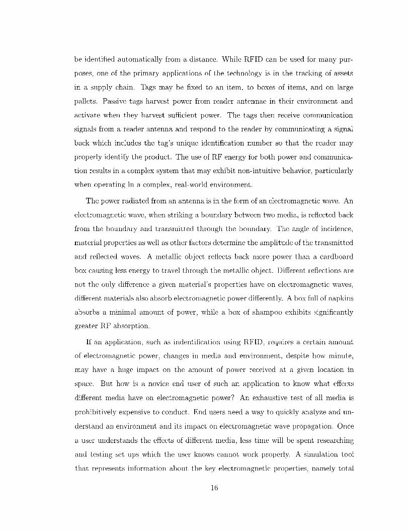
be identified automatically from a distance. While RFID can be used for many pur-
poses, one of the primary applications of the technology is in the tracking of assets
in a supply chain. Tags may be fixed to an item, to boxes of items, and on large
pallets. Passive tags harvest power from reader antennae in their environment and
activate when they harvest sufficient power. The tags then receive communication
signals from a reader antenna and respond to the reader by communicating a signal
back which includes the tag's unique identification number so that the reader may
properly identify the product. The use of RF energy for both power and communica-
tion results in a complex system that may exhibit non-intuitive behavior, particularly
when operating in a complex, real-world environment.
The power radiated from an antenna is in the form of an electromagnetic wave. An
electromagnetic wave, when striking a boundary between two media, is reflected back
from the boundary and transmitted through the boundary. The angle of incidence,
material properties as well as other factors determine the amplitude of the transmitted
and reflected waves. A metallic object reflects back more power than a cardboard
box causing less energy to travel through the metallic object. Different reflections are
not the only difference a given material's properties have on electromagnetic waves,
different materials also absorb electromagnetic power differently. A box full of napkins
absorbs a minimal amount of power, while a box of shampoo exhibits significantly
greater RF absorption.
If an application, such as indentification using RFID, requires a certain amount
of electromagnetic power, changes in media and environment, despite how minute,
may have a huge impact on the amount of power received at a given location in
space. But how is a novice end user of such an application to know what effects
different media have on electromagnetic power? An exhaustive test of all media is
prohibitively expensive to conduct. End users need a way to quickly analyze and un-
derstand an environment and its impact on electromagnetic wave propagation. Once
a user understands the effects of different media, less time will be spent researching
and testing set ups which the user knows cannot work properly. A simulation tool
that represents information about the key electromagnetic properties, namely total
16

power available at all spatial points of interest, graphically so that the information
is represented clearly and immediately would lead to a better understanding of the
technology and allow its uses to progress faster.
1.2 Introduction to Passive RFID
Imagine a stock room full of boxes filled with many different products; razor blades,
laundry detergent, etc. In this scenario there are a few ways to retrieve information
about the physical objects. The first is to manually view and record information, but
this is time consuming and prone to human error. Another way to retrieve information
would be through the use of computer vision or some sensing arrangement, but these
solutions are often expensive and inaccurate even for the most advanced systems.
RFID provides an inexpensive and efficient way to retrieve physical information. The
most inexpensive RFID systems use passive tags. Passive tags, unlike active tags, do
not use external power supplies such as batteries to supply their operational power,
but rather, receive their operational power from the tag reader's communication sig-
nal. This requires the tags to contain less functionality and consume less power than
active tags.
In an RFID environment, multiple reader antennae are placed at strategic loca-
tions to capture as many tag reads as possible. The readers then send out signals
into the environment requesting the identification number of any tags. These signals
are sent into the environment by emitting electromagnetic waves. The exact distance
and direction in which these waves are sent is based on the design and placement of
the reader antennae. The electromagnetic waves then propagate through the environ-
ment and may be reflected, absorbed and even interfere with each other. All of these
effects may cause the waves to end up at unexpected locations or with unexpected
amplitudes and phases.
The passive tags, which are affixed to items of interest, operate in a different
manner. The tags use an antenna and circuitry to receive electromagnetic power
from the reader. If their harvested power is above a minimum operating threshold,
17

the tags begin to operate and listen for communication signals from reader antennae.
What signal the tags are listening for is defined by a protocol which both the tags
and the reader antennae must adhere to. Once the tag receives a proper signal, it
then responds to the signal by back scattering some of the electromagnetic waves
that are incident upon it. The signal communicated back to the reader also adheres
to the same protocol as the signal sent from the reader. The back scattered waves
may again be reflected, absorbed or interfered with by other waves. Once the reader
antenna receives this signal, which contains the unique identification (ID) number of
the tag, the ID number is recorded and then processed by a well defined computer
infrastructure. While the system is easy to use, there are many places in which
problems can occur and there exist few tools which allow users to easily understand
an RFID environment in an intuitive manner. In general, getting sufficient power to
the tag is the bottleneck in communication with passive RFID tags.
1.3 Motivation for a Simulator
Passive RFID systems, like any other systems, are not without limitations. When
a tag cannot be read properly by a reader antenna, any number of factors could be
the cause. The tag could be using a different protocol, there could be interference
in the path between the tag and reader which causes signals to be misinterpreted, or
the most common problem is that the tag does not receive sufficient power from the
reader antenna to operate.
The passive tags need to receive a minimum amount of power from the reader
antenna to operate. Not receiving this power is a common problem with passive
RFID systems. The tags can be too far away from the reader antenna or the problem
can be more complex. The problem could deal with specifics about products within
a box or the environment in general. Certain products may allow the power to pass
through and permeate all through the box, while other products may reflect back
most of the power which might cause only certain areas of the box to have sufficient
power for a tag to be operational. Therefore, for certain products, the tags should be
18

located in specific areas of the box. Or the problem could not be with the products
themselves, but with the surrounding environment. Light fixtures, metallic walls, and
humidity in the air can all affect the way that electromagnetic power can propagate
through space. With a realistic simulation tool, an end user could understand which
sides of a box to locate a passive tag, or the user can come to the realization that
certain areas of the environment are "dead zones." Both of these conclusions can
be made quickly without expensive or exhaustive tests through the use of a good
simulation tool.
1.4 Description of Simulator
I have developed a software program which simulates specific aspects of an RFID
enviornment called RFID Vis. Its main use is in developing an RFID users' intuition
of how electromagnetic power radiates from reader antennae at UHF frequencies. To
quickly develop intuition, RFID Vis has a few key features. First, RFID Vis has an
intuitive user interface which allows users to create environments quickly and easily.
Menu driven actions create different items like antennas, tags and boxes of products.
Clicking and dragging these objects changes their displacements while dialog boxes
allow the users to change different properties of the objects as well. This intuitive
interface allows users to, through use of the standard keyboard and mouse, create
pallet like environments in which the properties of different boxes are quickly alterable
to show the effects that different materials have on the electromagnetic power radiated
by the antennae.
Another feature that allows RFID Vis to accelerate users' intuition of RFID is its
electromagnetics engine. The electromagnetics engine of RFID Vis allows for the user
to select between different electromagnetic approximation algorithms. Although at
the moment only one algorithm is implemented, in future versions of RFID Vis, other
algorithms may be available for use. Having multiple algorithms to select from as well
as control over certain aspects of the algorithms allows for users to control the speed
and accuracy of the results that are produced. If the users want very accurate results
19
or very quick results, they have control over the type of results RFID Vis produces.
Not only does the electromagnetics engine allow the user substantial control over
the accuracy and speed of the results produced by RFID Vis, but the engine also
produces real-time results. As previously mentioned, the users of RFID Vis have
control over the speed and accuracy of the results that are produced, but what if an
object in the scene is moved? If an object is moved, it has the ability to drastically
change the electromagnetic power over a given area, so when an object is moved
the electromagnetics engine defaults to using a real-time algorithm. If the user were
using an algorithm that took a few seconds or minutes to compute results, then it
would take minutes or seconds to move the object and see results. So, by defaulting
to a real-time algorithm, RFID Vis makes it quick to move objects around a scene
and adjust properties while at the same time not having the user doing this without
any feedback. The real-time algorithm provides results so that the user may see the
general effect that moving the object has while making the object movement be quick
and easy to use. Once objects are set in place, the user has the option of running
more accurate algorithms.
One last feature of RFID Vis that allows users to quickly develop intuition is that it
provides results and data quickly and in an easy to understand and three dimensional
manner. Unlike other electromagnetic software packages, RFID Vis provides very
specific information. While some software packages calculate and present a large
amount of data, the data most pertinent to RFID users is the electromagnetic power.
Therefore, RFID Vis provides the user with only the electromagnetic power, this
allows for faster calculations and faster algorithms. Specific power levels are mapped
to specific colors so that in a glance a user may note the power at a point within
a certain degree of accuracy and then these colors are drawn in three dimensional
space. The electromagnetic power is then rendered as a whole volume over space.
This allows for fast prototyping of results because the user no longer has a need to
rerun simulations.
Instead of needing to view many two dimensional graphs or only being able to
view two dimensional contours over a volume of space, the user now has access to see
20

a whole volume of data. RFID Vis allows the user to fully explore this whole volume
of data at any angle without needing to rerun any simulations. By rendering the data
in this manner, RFID Vis allows for fast prototyping and at a glance understanding
of results of a whole volume of data. This requires the user to rerun simulations less
and may cause less confusion than some other electromagnetics software packages;
the net result being that RFID Vis is easier to use and produces results more quickly
which leads the users to develop intuition about UHF RFID more quickly than other
software packages.
1.5 Thesis Summary
In this thesis I present the design, implementation, use and evaluation of RFID Vis,
a software tool that simulates specific aspects of passive UHF RFID environments in
real-time and presents data graphically. RFID Vis consists of many interconnected
systems and subsystems all of which are described in this section.
In Chapter 2, I describe the design of and previous work relating to the many
aspects of the user interface, known as the Intuitive Graphical User Inteface (I-GUI),
that is used in RFID Vis. The I-GUI combines many different tasks into one well
defined system. The I-GUI must interact with the user, respond to the user's inputs
and give the user feedback in an intuitive and graphical manner and must do so in a
flexible and easily extendible way.
The key design aspects of the I-GUI are to have the interface be extensible for
future use, intuitive to allow for faster creation of RFID environments and to represent
information in a easy to understand manner. By analysizing previously researched
topics of data visualization, previously implemented user interfaces, and carefully
detailed analysis of the problems facing the I-GUI, a design and a set of goals that
the I-GUI must accomplish was constructed and is discusse.
Chapter 3 bridges the gap from design to implementation as I discuss how the I-
GUI is implemented and how the implementation helps it reach its goals. The I-GUI,
which is responsible for a large number of tasks, is broken down into a number of
21

smaller systems within itself. One system is reposonsible for how objects (antennae,
boxes, etc.) are implemented and managed. Since RFID Vis is a continuing project,
these objects must share a common functionality while also allowing there to be new
objects intorudced without much change to the existing code base. Because of that
fact, the implementation and management of the objects is complex.
Besides objects being managed, the I-GUI must also respond to and receive user
input. What commands are received and the various responses to the different com-
mands are discussed in detail in Chapter 3 as well. One other topic discussed in the
chapter is the implentation of the visualization of computed data. There are many
ways to visualize data and for the specific data which is calculated in RFID Vis, there
were many different approaches to take into consideration. The chapter discusses the
chosen implementation, its advantages, disadvantages and tradeoffs.
In Chapter 4, I analyze and present the implementation of the I-GUI. One por-
tion of the chapter discusses the trade offs between different settings for the data
visualization. The visualization process is complicated and full of different aspects
which can be altered. The different settings have direct correlations to the speed and
appearance of the data visualization. A specific setting may produce the best looking
results, but unfortunately takes an amount of time to render which is too large so
that it hinders the real-time application of RFID Vis. A different setting or group
of settings may produce the quickest results but may not achieve the desired visual
effects. The trade off between settings and their effects on the data visualization are
discussed in Chapter 4.
Chapter 4 also presents how the implementation of objects and how the objects
are managed allows for the I-GUI to be easily extended. A carefully designed and
implemented system for handling objects can make addings new features and new
objects a breeze, but a poorly constructed system may cause lots of headache and
rewriting of code. The chapter discusses how the I-GUI avoids pitfalls and prevents
future headaches.
In Chapter 5, I describe, in detail, the challanges and design issues assosciated
with the electromagnetics engine "back end" of RFID Vis known as the Simulation
22
Engine. The Simulation Engine needed to be capable of many different key features
and the chapter discusses what those features are and how they were designed by first
consulting previous work done on the topic of electromangetic simulations.
In Chapter 6, I describe how the previously discussed designs are implemented
and brought into reality. How the abstract concepts of a real-time simulation as well
as an extendible engine were impleneted are presented in detail in the chapter.
Chapter 7 presents data as to how the running time of RFID Vis is affected by the
different settings and aspects of the Simulation Engine. How exactly do the different
parameters of a simulation affect the simulation time and what kind of behavior
is expected at certain levels of complexity? These questions are answered within
Chapter 7.
The final chapter, Chapter 8, presents conclusions about RFID Vis and its devel-
opment, usefulness and accuracy. Possible future expansions to the project are also
discussed.
There are many features of RFID Vis that allow its users to develop their intu-
ition of RFID technology and electromagnetic radiation quickly. An easily usable
user interface allows for scenes to be created quickly and easily. Customizable and
expandable electromagnetics algorithm parameters give the users control over how
accurate and quick results are calculated. Finally, RFID Vis displays data over a
huge volume of space which allows for the entire data to be visualized and deciphered
without recalculations. All of these features combined together allow for a scene to
be easily set up, data of different accuracy to be calculated and then the data is
displayed clearly and easily over a whole volume of space. These aspects of RFID Vis
make it easy to set up and test certain features of an RFID environment. This allows
users of RFID Vis to develop a better understanding of the environment.
23

24

Chapter 2
The Intuitive Graphical User
Interface
The code structure of RFID Vis consists of many interconnected objects working
together. The code can be divided into two main components, the Inuitive Graphical
User Interface (I-GUI) and the Simulation Engine. The I-GUI is made up of the
components of RFID Vis that directly interface with or can be seen by the users;
where as the Simulation Engine is responsible for "behind the scenes" work such as
computing electromagnetic power.
The I-GUI of RFID Vis is made up of many classes working together, but logically
the I-GUI consists of two main systems. One system creates and manages objects
inside an RFID environment such as antennas, boxes, and tags while the other system
renders each object in the environment and displays to the user each object's relevant
data. These two systems working together allow for RFID Vis to be controlled via
user input and display to the user the relevant information that is calculated.
2.1 User Interfaces and Their Challenges
A user interface is a piece of software whose function is that of what its name implies,
it serves as an interface between the user and the rest of the software. In more detail,
a user interface servers as a medium for retrieving input from the user and then
25
sending program output back to the user. The user interface is the interface between
the user and the program's functionality.
RFID Vis's main use is developing its user's intuition of electromagnetics and
RFID technology, so the user needs ample control over key aspects of RFID Vis. The
user needs to be able to create an RFID environment and manipulate it. The user also
needs control over certain simulation parameters to be able to specify the accuracy
and speed of the simulations that are run. While the users of RFID Vis need to be
able to control the simulations through some sort of input, the users cannot alter the
RFID environments well without some feedback from RFID Vis. Therefore, the user
interface needs to display to the user where each object is in the environment as well
as the electromagnetic power over specified volumes of space.
The main challenge that plagues user interfaces is that each application which uses
a user interface is very unique. A video game is very different from a spreadsheet
program in terms of the data that needs to be fed into and read out of the different ap-
plications. Because of this fact, user interfaces are not very portable from application
to application and a new interface must be written for every new application.
Each specific user interface has its own set of challenges. There are many objects
in an RFID environment that can be created in RFID Vis, and the user interface
needs to interact with each object in a specific manner. A box that can be stacked
on a pallet may need to be interacted with differently than a reader antenna since
each object has its own parameters that need to be altered. Futhermore, each object
has different data that needs to be presented to the user. The challenge faced by
the interface of RFID Vis was to develop a standardized way to properly interact
with an assortment of unique objects. A standardized method of input and output
needed to be developed which passed the control of the specific behavior down to each
individual object. This way, each object in an RFID environment implements the way
it responds to user interface events rather than a managing class assigning a behavior
to the object. Developing this standard interaction between the user interface and
objects which may be found in an RFID environment without needing very specific
code was a large challenge that was overcome during the development of the user
26
interface for RFID Vis.
2.2 Previous Work on Volumetric Data
While the user interface for RFID Vis had many challenges and issues to take into
consideration, one of the more complex challenges was how to render the electromag-
netic power radiated by a reader antenna since RFID Vis computes the power over a
whole volume of space.
Computer screens are two dimensional surfaces, so every image displayed on a
computer screen, despite what the image may be, is ultimately projected onto a two
dimensional surface. A problem arises when two dimensional geometries such as lines
and two dimensional datasets are not sufficient methods for representing the data
that an applications wants to present to a user. When the data to be rendered is a
volume of data, such as the electromagnetic power over a volume of space, rendering
this data to a computer screen is known as volumetric rendering and is a known
problem. Volume visualization or volume rendering is a method of extracting data
from volumetric data sets through interactive rendering[9]. Volumetric rendering has
been a topic of discussion and research in computer graphics for decades and there
are many different concepts and algorithms of how to map a volume of data to a
computer screen.
For the most part, volume data is made up of either scalar fields or vector fields.
For scalar fields, like RFID Vis has, two main algorithms come to mind: direct
mapping and iso-surface mapping which are discussed below [4]. The volume of data
may be well defined and structured or unstructured. The structured datasets contain
data at well defined sample points, while an unstructured set of data may be skewed
and psuedo-random [14]. Since the data computed by RFID Vis is defined as being
the electromagnetic power at a given set of points, the data computed is structured.
27

Figure 2-1: Example Voxel Grid
2.2.1 Voxel Based Direct Volume Rendering
One method of volumetric rendering is based on a collection of "cells" or voxels. A
voxel is a pixel taken into three dimensions as voxel is short for volume pixel. Voxel
based direct volume rendering takes the volume of data and directly maps the data
to a grid of voxels much like a Cartesian coordinate system[18]. An example grid
can be seen in Figure 2-1. The dimensions of the voxel grid and overall size of each
individual voxel is dependent on the application and each vertex of the voxel grid has
red, blue, green and alpha values. The data in the dataset is then directly mapped to
the vertices of the voxel grid through use of a color map; this mapping is implemented
differently in each application [8].
Once all data of the voxel grid has been computed, the next step of the rendering
process is to color each pixel of the computer screen based on the voxels in which
there are countless ways to do. One type method, known as forward mapping, maps
the data at each voxel to a set of graphical primitives which are rendered to the
screen in the data set's coordinate system [3]. These methods are straight forward
but require drawing many geometric primitives. Another group of methods, known as
backwards mapping, calculate the color at each pixel through some algorithm, such
as ray tracing, and then once all pixel colors are calculated one rectangle is rendered
in the screen's space giving the illusion of viewing a full scene [13]. These methods
28

require rendering only a few simple geometries but require a complex algorithm to
compute the pixel colors. The difference between the two types of method can be
thought of as the difference between being part of a scene and viewing a picture of
the same scene.
Whatever the method used, the colors displayed on the computer screen are based
on the data stored in a grid of voxels. One advantage of voxel based volume rendering
algorithms is that the volume dataset does not require a specific shape or contours; any
amorphous volume such as clouds or gases can be properly rendering using voxel based
methods. Another advantage is that the whole volume dataset may be represented
in the voxel grid as there may be a one to one mapping between voxel vertices and
dataset entries. A disadvantage is that every time an image is to be rendered, the
whole voxel grid must be traversed and there are possibly a large number of geometric
primitives to be rendered.
2.2.2 Surface Based Volume Rendering
Another method of volumetric rendering is based on two dimensional surfaces. The
idea behind surface based volumetric rendering is analogous to isolines on two di-
mensional graphs or that of feature extraction. The volume dataset is traversed and
similar data points or data points within certain thresholds are noted. Once all the
similar data points are collected, surfaces may be constructed based on those points
[18].
How these surfaces are constructed differs from application to application. Some
applications construct a single surface as a threshold value while other applications
may construct many surfaces to indicate points of similar data. Once all the surfaces
are calculated, the surfaces are then constructed out of geometric primitives and the
whole volume of data is no longer required to be kept available. These primitives are
rendered to a scene and then projected onto the computer screen.
One advantage of surface based rendering is that for each rendered image, only a
small subset of the whole volume dataset needs to be traversed as only those points
that are on the surfaces themselves are of note. Also, depending on the number of
29

surfaces as well as the surfaces themselves, a small amount of geometric primitives
are needed to render the surfaces. A major disadvantage of surface based rendering
is that not all datasets form well to surfaces. Some datasets have no required shape
or data points of similar values may be few and far between so constructing a surface
based on these datasets will just produce odd looking surfaces that give little to no
useful information to the user.
Direct mapping and surfaced based methods are not the only ways to render vol-
ume based data but are fairly common. New methods are constantly in development,
but each method will have its advantages and disadvantages and each method will
ultimately map the data in a volume dataset to a color that needs to be displayed on
the computer screen.
2.3 I-GUI Design and Goals
When designing the I-GUI, the most important aspect of the design is meeting the
extensibility and usability goals of the I-GUI. The goals of the I-GUI were that the
I-GUI needed to be extendible so that future work on RFID Vis may add objects to
the I-GUI without needing to change too much preexisting code and the I-GUI also
needed to be user friendly and intuitive. The I-GUI must also contain items which
can be used to visually display to the user certain data that is calculated by the back
end about objects in the RFID environment. Extensibility is one of the characteristics
of well designed code [15].
2.3.1 I-GUI Extensibility
While the current implementation of RFID Vis takes into account certain objects
for a packaging related RFID environment, it is not unrealistic to think that the
electromagnetic simulation aspects of RFID Vis could be used for different environ-
ments besides the boxes and pallet environment currently implemented. So, to ensure
the ease in creating new and different environments, the I-GUI was designed to be
moderately extensible with regards to new objects.
30

To accomplish this, each object in the RFID environment follows and must imple-
ment a standard interface in which the management classes are used to manage the
RFID environment. Each object must define a method to render and update itself as
well as respond to a defined set of user actions. The actual implementation of these
methods is up to the objects themselves, but the method calls and general interface
to these methods is well known. In doing this, RFID Vis can easily be extended to
contain new objects beyond those included in the current implementation.
For example, if in a future version, a Tube object is added to the RFID environ-
ment, minimal code would have to be altered or added. A Tube class would need to
be defined that extends the generalized RFID environment object. The Tube would
then need to define its own render, update and user action related methods. One
other piece of code would need to be changed within RFID Vis to add a way for the
user to create the Tube object, but that is all. So, to add a whole new type of object
with its own unique behavior, a minimal amount of existing code would need to be
altered and a whole new stand-alone class would need to be created. This makes ob-
ject creation for future versions of RFID Vis easier and allows for new object creation
with minimal changes to the code base.
The effect of this is that future developers of RFID Vis will not be required to
know intimate details of the existing code base to add new objects to the environment.
To extend RFID Vis and create a new object, one needs only know the general
"environment object" interface.
2.3.2 I-GUI User Interaction
No matter how good of an architectures may be designed, if the user has to go
through complicated procedures to input commands, the user becomes frustrated. If
a program becomes frustrating, the key features of a program may never get used
frequently or at all. It is better if the user interactions are quick, easy to understand
and intuitive as this allows for the user to use the program's features faster and more
frequently therefore maximizing the program's usefulness to the user.
RFID Vis has controls which have a low learning curve and have intuitive affects
31

which makes RFID Vis easy to use and better enables the use of itself. Some termi-
nology first, a Camera object represents literally a video camera from which the user
is viewing the virtual world created by a program. A program may have any number
of Camera's although most just have a single view point; RFID Vis contains only one
Camera object. The controls for the Camera are set up in a fashion similar to those
of a first person shooter game such as DOOM. Keyboard (or mouse) buttons move
the Camera forwards or backwards along the Camera's line of sight. Other buttons
move the Camera laterally along an axis that is perpendicular to the line of sight and
in the plane of the screen. Other commands adjust the angles at which the Camera
views the world. One command changes the vertical angle while another one changes
the horizontal angle of the Camera. These movement commands can be bound to
any key, so a user can specify the keyboard layout of these commands so that they
may choose a setup that is most comfortable and intuitive to them.
Besides the Camera movement controls, there are a few other commands that the
user has over objects in RFID Vis. The first command uses the mouse to select and
drag an object via left clicking and the familiar drag and drop interface. When an
object is clicked, it is "selected" and certain data about that object is presented to the
user. When clicking on an object, the user may hold down the left mouse button and
drag the object. Upon dragging the object, the objects "drag" interface is invoked
and the object responds in some manner. Many objects may not respond to drags,
while others may adjust their displacement based on the movement of the mouse.
When the user right clicks on an object, the object invokes a command to display its
properties dialog. While the behavior of the objects and how they respond to these
commands may change from object to object, the buttons are not changeable and
these commands are permanently bound to the left and right mouse buttons.
With a very limited number of commands, RFID Vis has a very easy to use
and able understand input/output interface. Users only need to understand how to
use and manipulate a small number of movement commands for the Camera and the
specific workings of each individual object. By having such a low learning curve, users
of RFID Vis are more quickly able to create and manipulate complex environments
32

and this will quicken their intuition of UHF RFID propagation.
33

34

Chapter 3
I-GUI Architecture and
Implementation
The I-GUI is made up of many classes and objects working together. While the I-
GUI consists of many classes, logically it can be thought of as distinct packages, one
package consisting of RFID interface renderables, one package consisting of objects
in an RFID environment, and another package to manage all of renderable objects in
a "'scene."l
3.1 Environment Renderable Classes
When developing a graphical simulation application, one of the main features of it are
graphical in nature. It makes sense that a substantial number of objects would be ob-
jects that are drawn to the computer screen. Also, RFID Vis may be used to simulate
a number of RFID environments, RFID Vis needed to be generalizable and extensible.
To have such generalizable behavior and extensibility, object oriented programming
techniques were needed to develop an inheritance hierarchy which placed object im-
plementation specifies down the hierarchy and that defined a standard method for
interacting with the renderable objects. The following is a list of objects which are
part of the RFID Vis's set environment classes.
1. Camera Class The Camera class represents a camera from which a user can
35

view the RFID environment.
2. Renderable Class This class defines a standard interface in which an arbitrary
object may be drawn to the screen.
3. SelectionBracket Class Visually indicates to the user which object the user
has selected via user input.
4. SelectionInfo Class This object is used to present to the user some informa-
tion about the currently selected object.
5. CoordinateAxes Class This class represents axes in three dimensional space
at right angles to each other.
3.1.1 Renderable Class
At the top of the class hierarchy is the Renderable class. This class defines a standard
interface to render to the computer screen as well as the ways to allocate and free the
resources needed to accomplish the rendering.
Since RFID Vis uses the DirectX API as its interface to the graphics hardware, the
Renderable class uses a setup similar to that of predeveloped DirectX classes. When a
graphics device changes properties of a viewing window, such as changing a window's
resolution or size or changing the device type being used, the window is said to be
"restored" and all objects to be rendered to the device must be restored for this new
device settings. Therefore, a Renderable object has a restore method which which
takes a Direct3D device as a parameter. When properties of a window or device are
changed, the window and all objects to be drawn to it must be restored to work with
the new device and window settings; the restore method insures that all objects to be
rendered to the screen are restored and validated to use the proper device settings.
An invalidate method is also defined so that the resources that a Renderable object
allocates to properly render itself can be freed. An object is invalidated before it is
deleted or restored to a new device.
The key aspect of a Renderable object is that it represents an object which can
be rendered to the screen, so it follows that a Renderable object has a method called
render which handles the function calls to actually draw the object to the screen. The
36

render method is passed as a parameter a RENDER-PASS which describes what type
of rendering to do. There are many types of passes such as an OPAQUE-PASS which
renders only the opaque aspects of the objects. Also, an Renderable object has an
update method which takes as a parameter a floating point number which represents
a timestep to update by. The update method allows an option for a Renderable object
to vary with respect to time.
The Renderable class is a virtual class. Each of its methods is purely virtual as
the class itself only defines a behavioral interface for other classes to inherit from and
extend. Most of the other objects which are part of the I-GUI ultimately inherit from
the Renderable class.
3.1.2 Geometry Class
The Geometry class serves as a utility class that defines some general geometric struc-
tures as well as some general geometry related functions which may be used and are
useful for a number of situations. The class also is used as a wrapper which de-
fines higher level structures that wrap over predefined DirectX structures for vectors,
quaternions and matrices.
3.2 Physical Objects
One of the major concepts in developing any environment is the concept of a physical
entity which will be rendered to the screen. While the I-GUI may render any number
of objects to the screen as part of the user interface, the actual RFID environment is
constructed from many real objects such as antennae, tags and boxes which can be
stacked next to and on top of each other to form pallets. These objects have a physical
structure and make up the environment in which RFID Vis will be simulating. A list
of PhysicalObject based objects is seen below.
1. PhysicalObject Class The PhysicalObject class is a Renderable object which
represents a physical entity in RFID Vis which has a physical structure.
37

2. Reflector Class A Reflector is a special type of PhysicalObject which has
electromagnetic properties and which may affect the electromagnetic power in
an RFID environment.
3. Antenna Class The Antenna class represents a standard UHF reader antenna.
4. Floor Class The Floor class models a standard cement floor found at ware-
houses.
5. MaterialBox Class A MaterialBox object is a Reflector object that represents
boxes of product that are used to make pallets in a supply chain.
6. Tag Class The Tag class represents a standard passive RFID tag that can
adhere to boxes of product.
3.2.1 PhysicalObject
The PhysicalObject class is a Renderable object which represents a physical entity
in RFID Vis. The class outlines an interface in which the user can interact with the
objects as well as standard features of each object.
Each PhysicalObject has a linear displacement and a linear rotation. The linear
displacement is a three dimensional vector in world space, measured in meters from
the origin of the scene. The linear rotation of an object is represented by a quaternion
from which a rotation matrix can be calculated from. By using both the linear
displacement and rotation, a 4x4 matrix can be computed for each object known as
the transform matrix which can be used to transform a vector from world space into
the object's space.
Besides a displacement and a rotation, each PhysicalObject has an ID number.
This number should be unique for each PhysicalObject within a scene, but the man-
agement of ID numbers is not a task for each PhysicalObject. Since certain objects
in a scene may depend on another object's properties, such as a passive RFID tag
adhered to a box is placed on the surface of the box, so the tag in a way depends on
the properties of the box, each PhysicalObject has one and exactly one parent Phys-
icalObject in which it depends. While having multiple parent objects may not be
unreasonable, it is somewhat unrealistic. To keep the parent/child hierarchy simple,
38

each PhysicalObject can only have one parent PhysicalObject. A PhyiscalObject is
not required to have a parent object. A PhysicalObject also stores a collection of
its children PhysicalObjects since an object can have multiple children. Every child
object should have a parent and that parent should have that child within its list of
child objects.
One goal of RFID Vis is to be able to save an environment setup and reload the
setup at a later point in time. For this to happen, each object in an environment
or "scene"l must be able to be serialized and written to a data stream. Serialization
is a process in which all the high level data structures are taken down to the byte
level and a stream of bytes is written to a data stream. Since each PhysicalObject is
serializable and written to a data stream, each object must also be deserializable and
be read and reconstructed from a datastream. So, each PhysicalObject has a serialize
method and each PhysicalObject class has a static create method. Both methods take
a data stream as a parameter, the serialize writes the object to the stream while the
create method creates a new object based on the data stream.
As mentioned before, a PhysicalObject serves to represent an physical entity
within RFID Vis and the user is able to make adjustments to the setup of the RFID
environment, the PhysicalObject class defines an interface for generalized behavior
which may be linked to user input. Each object has a dialog known as its properties
dialog which it displays to its parent window. The structure and content of this dialog
vary with each object, an example of one can be seen in Figure 3-1.
The PhysicalObject class also outlines behavior to user "drag" actions as well
as "picking" functions which note if a ray from a given point traveling in a given
direction intersects the object.
While the PhysicalObject class does define and implement some standard behavior
that is consistent across all PhysicalObjects, mot of the methods defined, such as the
serialize and pick methods, are defined as virtual to pass the implementation further
down to the specific objects themselves.
39

Figure 3-1: Example Properties Dialog
40

3.2.2 Reflector Class
A Reflector is a specific type of PhysicalObject which has electromagnetic properties
that affect the electromagnetic power radiated by antennae. Reflectors and only
Reflectors are taken into consideration when the electromagnetic algorithms computed
the power over a given volume of space. All other objects in the scene are not taken
into account in the algorithms.
All Reflectors have three floating point number which represent three specific
electromagnetic constants which dictate their behavior in regards to how the Reflec-
tors affect electromagnetic waves. These constants are the electric permittivity of an
object, c, the magnetic permeability of an object, y and its electrical conductivity,
sigma. The current implementation has these electrical properties being constant
throughout each Reflector making each Reflector a homogeneous material. Future
implementations could change this behavior.
3.2.3 Antenna Class
The Antenna class represents a standard UHF reader antenna. An Antenna can
be of one of many AntennaTypes and PolarityTypes. The AntennaTypes dictate
the directivity of the Antenna object while the PolarityTypes affect the polarity
of the object. In the current implementation, there are two AntennaType values,
ISOTROPIC and PATCH. If the Antenna has an ISOTROPIC AntennaType, then
its directivity is consist with that of an isotropic antenna. While an isotropic antenna
is not physically possible, it is the bases of a lot of measurements of power and gain of
common antennae. There are two values of PolarityTypes which represent linear and
circular polarizations. The AntennaType and PolarityType are the only changeable
parameters that affect the electromagnetic behavior of an Antenna.
The Antenna class, stores in a three dimensional grid of points, the complex
electric and magnetic fields at that point in space. The fields are stored as real parts
and imaginary part and stored as three dimensional vectors. The vector direction
indication the direction of the field and the magnitude indicates the strength of the
41

field at that point.
The exact size and number of points in this "grid" is controlled by a few parame-
ters. Each Antenna object is given a set of parameters to describe this grid of points.
An Antenna is passed a width, depth, and height and a parameter of points per me-
ter, all of which are integers. The width controls the total width along the Antenna's
x-axis in which the grid extends, the height controls the y-axis extent and the depth
controls the z-axis extent. In the x and y axes, the width is taken across the center of
the Antenna. So, if a width of 5 meters is specified, the the Antenna has grid points
which represent the the electromagnetic power up to 2.5 meters right and left of the
center of the Antenna; the y-axis would have the power measured up to 2.5 meters
above and below the Antenna. On the z-axis however, the depth is taken from the
Antenna out. This has the Antenna always having the electromagnetic power in the
"forward facing" direction as any power behind it is not stored.
3.2.4 Rendering Antenna Power
When it comes time to render the transparent aspects of an Antenna object, the An-
tenna needs to render the electromagnetic power over its designated volume of space
which is stores the electromagnetic field. Every Antenna, as mentioned above, stores
the electric and magnetic fields over a whole volume of space in the vertices of a three
dimensional "grid." Given this grid structure of storage used by the Antenna, voxel
based volumetric rendering would seem to be the most applicable way of rendering
the volume of data.
The first step in rendering the Antenna's power is to convert the voxel data to
colors that can be used for rendering. The data stored by an Antenna is the electric
an magnetic fields over its given grid volume, but the data that the simulation wants
to render to the screen in its current implementation is the time-average power, not
the electric and magnetic fields. The time-average power can be found using the
electric, E and magnetic, H, fields. The time-average Poynting vector, S, for a given
42

wave is calculated to be
(S) = -R(E x H*) (3.1)2
The time-average power density is then given by
(IS) = -R[J x H*J] (3.2)2
Once the power density at each point is calculated, a color lookup function produces
an RGBA color based on the power density at each point; all power densities are
assumed to have no time dependence, so they are simply the time average power
densities. Each of these colors is then stored in a three dimensional volume texture.
In the end, the color of each texel in the volume texture corresponds to power level
at each point of the "grid" that is stored in each Antenna object.
The next step in rendering the power associated with the Antenna object is find-
ing geometry to render to the screen and associating the geometry with the volume
texture. The approach taken is a standard approach to volume rendering that has
been around for years. The geometry for rendering the volume are "slices" of the
complete volume. The idea is to apply the volume texture onto cutting planes or
"slices." These slices can be of any orientation, but the Antenna object uses object
aligned or image oriented orientation of the cutting planes so that the cutting planes
are parallel to the axes of the volume of data. An example of slices aligned with one
single axis can be seen in Figure 3-2. There are however, three sets of these slices,
one for each axis of the Antenna object.
The advantage of having the cutting planes be axis aligned is that the imple-
mentation in the software is more straightforward while only costing a little bit of
rendering computation. Using the axis aligned cutting planes can lead to a "popping
effect" when the slicing axis changes. When this happens, it is possible that the
image intensity changes as the viewing angle may now be viewing a different number
of slices then at a previous viewing angle. While using axis aligned slices can create
small visual artifacts that may not exist with other alignments such as view angle
slice alignment, the simplicity of the implementation and lack of complex calculations
43
Lj
Figure 3-2: Axis Aligned "Slices" for a Single Axis
is why the axis aligned method of orientation was chosen.
When the slices are rendered to the screen and alpha blending is enabled so that
more than the front slices are visible, an illusion is given so that it appears that the
whole volume of data is rendered to the screen. In reality the cutting planes form
a series of rectangular prisms with no data inside the "cells." The more frequently
sampled the volume data, the smaller the spacing between slices and the more realistic
the volume of data appears.
One down side to this rendering algorithm is that it requires a lot of texture
memory. Depending on the side of the data set and the size of the volume of space
to render over, the textures created and used could take up huge chunks of RAM.
On older, less capable machines, this could cause an extreme slow down or even out
of memory errors. Fortunately, most of the data sets and fields in which RFID Vis
will feasibly be run in will not even remotely begin to scratch the surface of these
limitations. The textures do however, still take up a large section of RAM currently;
this is an area which may need some optimizing.
44

Figure 3-3: A Tag object that is "off" and "on"
3.2.5 MaterialBox Class
A MaterialBox is a Reflector that is a box filled with a specified material with specific
electromagnetic behavior. A MaterialBox represents a box filled with product that
are usually stacked together on pallets in warehouses and loading docks that are used
in a supply chain. A MaterialBox may be filled with predefined a BoxMaterial or
may be filled with a "custom" material that is specified by a few electromagnetic
constants. A MaterialBox is placed on a Floor and when dragged, the MaterialBox
moves along the axes of the Floor.
3.2.6 Tag Class
The Tag class represents a standard passive RFID tag. A Tag is attached to the
face of a MaterialBox upon creation and moves along the surface of the MaterialBox
when dragged. Other classes specify to a Tag the available electromagnetic power
around it. The Tag reads in the power given to it and compares that power level to
a specified minimum threshold power. If the read in power is above the minimum
threshold, then the Tag "turns on" and gives some indication to the fact that the
Tag is on. The visual difference between an "off" Tag and an "on" Tag can be seen
in Figure 3-3. The on/off state of the Tag may be toggled as the power read in may
fluxuate at being above or below the minimum threshold.
45

3.3 Environment Management Classes
While objects that may be drawn to the screen make up a large portion of the I-GUI,
the I-GUI also consists of a collection of classes that manages the other classes, feeds
the other classes input from the user and passes information between classes. A list
of classes which are in the set of environment Management classes is given below.
o Scene Writer Class The SceneWriter class takes a "scene" from RFID Vis
and writes the scene to a file. All the objects in the scene are serialized and
written to the file whose filename is specified to the class and the objects are
written in order of the parent/child hierarchy.
o SceneReader Class The SceneReader class reconstructs a "scene" for RFID
Vis based on data read in from a file. All the objects in the scene are deserialized
from information read from the file whose filename is specified to the class.
o Packing Class The Packing class serves as the entry point to RFID Vis as well
ass interfacing directly with the Direct3D and DirectInput APIs. The Packing
class serves as a bridge between low level hardware and API issues and the
higher level issues specific to RFID Vis.
o SceneManager Class The SceneManager class manages everything about an
RFID environment "scene." It keeps track of different objects within RFID Vis
and serves as a bridge between the I-GUI and the Simulation Engine of RFID
Vis. The SceneManager class is the "brain" of RFID Vis.
3.3.1 SceneManager Class
The SceneManager class serves as the center of RFID Vis. It is in charge of "man-
aging" the RFID scene and acts as a bridge between the I-GUI and the Simulation
Engine. Most data that is passed through RFID Vis from class to class, object to
object is passed through the SceneManager at some point in time.
One priority of the SceneManager is to keep track and store the different objects
in a scene, so the SceneManager naturally has to store in a collection, all of the
PhysicalObjects in a scene as well as any other objects of special interest. When
46
certain commands or updates are received, the SceneManager sends the appropriate
data to the appropriate places. For example, when the SceneManager gets a signal to
render the scene, it calls the render function of the appropriate objects while setting
the viewport to its appropriate size and setting many other parameters. While the
actual controls of how each object is rendered is placed down at the object level, most
of the other parameters such as setting coordinate systems, and priming the system
to be able to render the object falls to the SceneManager.
The SceneManager also passes information between different systems of RFID
Vis. The back end of RFID Vis runs simulations, but does not know when they
need to be run. The back end does not keep track of the algorithms and calculates
electromagnetic power. The SceneManager must check the environment and note if
a simulation needs to be rerun or if a new simulation has been requested. If either of
those states are true, then the SceneManager requests that the back end run a new
simulation with the specified parameters.
Many of the systems that exist in RFID Vis were developed to accomplish a
certain task or a collection of tasks. These systems are unaware of the existence
of other systems that may exist. This makes the implementation of RFID Vis as a
whole behavior very modular which allows for future additions to RFID Vis to be
easier to make because systems have less dependencies on already existing code. Since
there are less interdependencies between existing code, extending RFID Vis requires
minimal knowledge of the existing implementation of the system.
3.3.2 Other Environment Management Classes
The SceneManager class is the only class presented in detail here as the other envi-
ronment management classes are sufficiently described in the sentences found in their
listings earlier.
47

48

Chapter 4
Analysis of the I-GUI
The I-GUI has many modules which could be implemented in a variety of ways. This
section will discuss the advantages and disadvantages of the current implementation
as well as analyze the effect that certain parameters have on the speed of RFID Vis.
4.1 I-GUI Usability
A large portion of the I-GUI consists of the user interface in which the user directly
interacts with. One of the key features of the user interface is the customizability of
the key bindings with regards to Camera movement. While the default key layout
for the different Camera movement commands are very well placed, the user has the
option to changing the key bindings of the different movement commands so that the
key layout may be what the user prefers. This customizability makes the Camera
movement controls very user friendly. The Camera movement controls have a slight
learning curve as they take a few minutes to grasp. The control are very analogous
to standard first person shooter games like DOOM or Quake's commands, so if the
user has played those games, the learning curve is small. While the controls are
decent and easy to manipulate once the user gets the hang of them, they still leave
something to be desired as on a few occasions to change the Camera position a very
small distance to get a better view of the scene, the user may need to go through
a long series of commands to change the position and viewing angle slightly. Also,
49

the Camera movement commands have a set minimum amount they can move in a
particular direction. If the user wants to move less than this amount, it is impossible
for the user to do this. While the minimum is relatively low and in general does not
cause problems, it may still cause minute problems. The Camera movement in RFID
Vis is easily bound to any key which allows the user to specify a particular key setup.
The Camera controls are a major way in which the user interacts with RFID Vis,
but not the only way as the user can also manipulate objects in the environment. The
method that the user have for manipulating the objects involves the use of the mouse.
The user may left click an object to select it, left click and drag an object to activate
the object's drag command, double click to zoom to the object, or right click to bring
up the object's properties dialog. These commands work well and are pretty standard
and easy to understand, unfortunately, unlike the Camera movement commands, the
object manipulation commands cannot be freely bound to any input device; they are
permanently bound to the mouse. The left click will always be the selection and drag
button, while the right click will always bring up the object's properties dialog. The
controls to manipulate objects are simple, but unfortunately, the buttons to control
the object cannot be changed, so the user is stuck with the default buttons for these
controls which limits the customizability of RFID Vis.
Another problem with the object manipulation commands is that every object
has a different drag command and a different properties dialogs and it may take
the user a few uses to memorize how the different objects react when dragged and
what properties the different objects have which may be manipulated. While there
are a relatively low number of unique object types, there does not exist a standard
set of commands or actions. One object may respond to a drag by adjusting its
position based on the Camera movement along certain axes while another object may
be moved along a completely different set of axes or the drag command for a given
object may be to rotate the object or some other command. The problem is that
there is not a standard set of commands, so the user does not really know what to
expect and must experiment with the objects to figure out what their drag commands
are and what properties can be adjusted through the properties dialog. This problem
50

of inconsistent commands is not a large problem, but it does make the user have to
experiment a bit to become accustomed to the different behaviors of the different
objects.
The properties dialogs which are brought up for each object via right clicking
on the object are also a cause for little concern. The dialogs are relatively straight
forward, but the correct type of data to enter into some of the edit boxes is not that
straight forward. Some properties are based on numbers and these numbers can be
floating point numbers or integers depending on the object and the property. The
problem is that the edit boxes allow the user to enter any sort of data and only upon
clicking the "OK" button does the data get checked for proper data type and proper
data. A better feature would be to indicate to the user what type of data to enter
into the edit boxes, but that feature is not available in RFID Vis. This causes the
user to have to experiment as to which properties take integer numbers and which
properties take floating point numbers. While this is not a large problem, it is a
slightly aggravating aspect of RFID Vis.
Overall, the user interface of RFID Vis is easy to use and intuitive which makes
it easy for the user to quickly create and manipulate RFID environments for use in
RFID Vis, but the user interface is not without its problems. While some commands
may freely be bound to any key or input device, other commands are permanently
bound to mouse input. Also, objects may behave differently to different commands
and there is no indication as to how the objects react, so the user is left to experiment
to determine the behavior of different objects. The same occurs with objects' property
dialogs as there is no clear indication which properties require integer numbers and
which properties require a floating point number; the user is left to experiment with
the different properties to find out which data types are required by the different
properties. These flaws with the user interface are small as most of the flaws are
easily worked around with a few minutes worth of experimenting with RFID Vis, but
they are flaws nonetheless.
51

4.2 Analysis of Electromagnetic Power Rendering
While a large portion of the I-GUI is the user interface, another portion of it is the
rendering the different objects in an RFID environment. While rendering most of
the objects is straight forward, the rendering of the Antenna object, as mentioned
in Section 3.2.4, is slightly more complicated as the rendering of the electromagnetic
power uses a volumetric rendering procedure to produce useful and good looking
results. The volumetric rendering algorithm used in rendering the electromagnetic
power has many parameters which affect the rendering speed of the algorithm as well
as how the electromagnetic power appears to the user. This section analyzes and
discusses the effects that altering a few parameters has on the underlying algorithm's
speed and results.
4.2.1 Texture Slices
The volumetric rendering algorithm described earlier uses a voxel grid and axis-
aligned slices when rendering the electromagnetic power. The axis-aligned slices are
aligned along the three major axes of the Antenna object, slices for a single axis may
be seen in Figure 3-2, and there exists a constant which defines the number of slices
which are used along each axis. The higher the number of slices, the more planes and
textures are required to be drawn which produces a better looking result because the
planes sample the data. The higher the number of planes, the more often the data
is sampled and it becomes harder to recognize the fact that there are distinct planes
being rendered to the screen, the region of space looks more like a more continuous
set of data. Therefore, the higher the number of slices per axis, the better the data
set looks, but unfortunately more geometry is required to render the electromagnetic
power which causes the algorithm to slow down.
A balance between speed and looks is a must and to find a good balance, a to find
an appropriate balance, some tests and analyses needed to be run. A simple RFID
environment consisting of solely an Antenna object was created and the number of
slices was altered and the average number of frames per second were recorded; the
52

Antenna's type was that of a patch antenna. These tests were all run on the same
machine with the same Camera placement to remove many inconsistencies. The
reason for having only an Antenna object in the environment is to ensure that most
of the computation time is spent rendering the power and not in any electromagnetic
simulation. One simulation should be run when the Antenna is first inserted, but
since the Antenna will not be moving, any computation spent after that will solely
be for rendering the electromagnetic power.
The rendering algorithm has a linear complexity dependence on the number of
slices used per axis. Increasing the number of slices per axis by one requires the
algorithm to then draw twelve more triangles to the screen as there are two triangles
per plane, two planes per slice and three separate axes to add slices to. Adding
additional slices also requires a bit more computation to texture map the slices as
well as alpha blend them all together. If the rendering algorithm is not using a
volume texture, than each additional slice also requires an additional texture to be
created and stored which uses a bit of computation and storage space. For a given
number of slices per axis, s, the volumetric rendering algorithm used renders 3s slices
or 12s triangles to the screen. There may be some additional computation or storage
required for each slice, but these constants can largely be ignored. The volumetric
rendering algorithm has a linear complexity dependence on the number of slices, s,
so the algorithm is said to be of the order 0(s).
All tests were run on a Pentium 4 2.0 GHz machine running windows XP profes-
sional with 1 GB of RAM and an nVidia GeForce FX 5200 video card. The results
of the volumetric rendering slices test can be seen in Table 4.1 and a graph of the
results can be seen in Figure 4-1. As expected, the rendering time for a given frame
increases as the number of slices increases because there are more geometries to ren-
der and more textures to compute. Figure 4-1 shows that the growth is roughly linear
with the number of slices which is consistent with the order of growth dependence
mentioned earlier.
The time to rendering a frame is not the only important aspect considered when
deciding on the correct number of slices to use, the data rendered also needed to
53

Number of Slices Milliseconds to Render
8 26.7216 43.6124 59.7332 76.9840 93.72
Table 4.1: Effects of the Number of Slices on Rendering Times
Rendering Times for Different Volumetric Slice Values (Single Antenna Only)100
9
8
W
CL
a)
Ec
6
5
3
0-
0-
0-
0-
0 -
0
0
10 15 20 25 30Number of Slices per Axis
35 40 45
Figure 4-1: Graph of Rendering Times for Different Numbers of Slices
54
5
V)
.E 7

Figure 4-2: Electromagnetic Power Rendering with 8 Slices per Axis
look decent. A screenshot of the rendered electromagnetic power using only 8 slices
per axis can be seen in Figure 4-2 and a screenshot using 32 slices can be seen in
Figure 4-3. One can see that when using only 8 slices, the results may be rendered
to the screen quickly, but the data loses a sense of being a whole volume as it is
fairly obvious that planar slices are rendered to the screen. As the number of slices
increases, the use of planar slices becomes less apparent and the data looks more like
a whole volume. I then decided that using 24 slices per axis looked sufficiently like a
whole volume and had a decent rendering time, so a value of 24 slices per axis was
used. A screenshot using 24 slices can be seen in Figure 4-4.
4.2.2 Texturing Methods
The number of slices used in the volumetric rendering of the electromagnetic power
affects the speed of the rendering process more than most other parameters, but
there are other parameters which also affect the speed of the rendering. One of these
parameters is the texturing method used when rendering. As mentioned before, the
55

Figure 4-3: Electromagnetic Power Rendering with 32 Slices per Axis
Figure 4-4: Electromagnetic Power Rendering with 24 Slices per Axis
56
.... .. .......
actual geometries rendered to the screen are a collection of parallel two dimensional
planes, but to have these planes be colored correctly, the electromagnetic power data
is mapped to either a three dimensional volume texture, or a set of two dimensional
textures and the textures are then mapped to the geometries themselves.
The reason for having different texture types (the volume texture or traditional
set of two dimensional textures) is that not all video hardware available on the market
have the capability to use a volume texture, so for RFID Vis to be compatible with
all sorts of hardware, RFID Vis dynamically switches between using a three dimen-
sional or set of two dimensional textures based on the current hardware being used.
Although RFID Vis automatically defaults to using a volume texture if applicable, it
is possible, by changing some source code, to force RFID Vis to use a certain type of
texturing method.
Using the volume texture, creates a very large texture in which the slices have
three dimensional texture coordinates which map the texture to the slices, so each
vertex requires three texture coordinates and the volume texture itself requires a large
amount of memory to be stored. On the other hand, using two dimensional textures
requires only two texture coordinates for each vertex, but unfortunately the two
dimensional texture approach requires that three two dimensional textures are stored
for each slice (one per axis) and some of the textures overlap which causes the same
information to be stored on two or three textures instead of a single texture. Using
two dimensional textures seems like a slightly inferior solution, but two dimensional
textures have been in existence for quit some time and the hardware for mapping two
dimensional textures has been highly optimized while volume textures are relatively
new and the graphics hardware may be unoptimized for using volume textures; each
method has its advantages and disadvantages.
To show the affects of the different texturing methods on the rendering speed and
look of the rendered electromagnetic power, the same test environment was used that
was used when testing the affect of using different numbers of slices which involved
solely an Antenna object. Using this test file, the average milliseconds needed to
render a frame were recorded using the two different texturing methods. The results
57
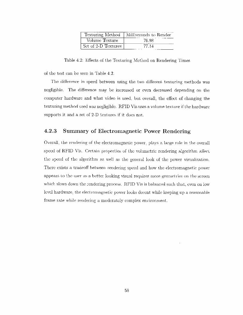
Texturing Method Milliseconds to RenderVolume Texture 76.98
Set of 2-D Textures 77.14
Table 4.2: Effects of the Texturing Method on Rendering Times
of the test can be seen in Table 4.2.
The difference in speed between using the two different texturing methods was
negligible. The difference may be increased or even decreased depending on the
computer hardware and what video is used, but overall, the effect of changing the
texturing method used was negligible. RFID Vis uses a volume texture if the hardware
supports it and a set of 2-D textures if it does not.
4.2.3 Summary of Electromagnetic Power Rendering
Overall, the rendering of the electromagnetic power, plays a large role in the overall
speed of RFID Vis. Certain properties of the volumetric rendering algorithm affect
the speed of the algorithm as well as the general look of the power visualization.
There exists a tradeoff between rendering speed and how the electromagnetic power
appears to the user as a better looking visual requires more geometries on the screen
which slows down the rendering process. RFID Vis is balanced such that, even on low
level hardware, the electromagnetic power looks decent while keeping up a reasonable
frame rate while rendering a moderately complex environment.
58

Chapter 5
The Simulation Engine
The Simulation Engine works in a quite different manner than the I-GUI. While the
I-GUI is seen by the user and receives input from and displays data to the user, the
back end is never seen by the user. While the back end may respond indirectly to user
input, the user has little to no knowledge of the Simulation Engine and its workings,
just solely of the results it produces. The Simulation Engine of RFID Vis produces
the results that are eventually shown to the user; the Simulation Engine runs the
simulations for RFID Vis.
5.1 Introduction to Electromagnetics Engines
The definition of a software engine is a piece of software that encapsulates a large
amount of computation, but cannot be used without some kind of front end. So,
an electromagnetics engine is an engine which calculates, through a large amount of
computation, a result that simulates the behavior of electromagnetic phenomena.
What results are ultimately computed and how they are computed are part of the
engine design itself. Some engines calculate a myriad of data, while other engines
may produce a smaller number of results. Another aspect of an engine is flexibility.
Certain engines may produce different results based on formal parameters that are
passed to it. Also, even if engines produce the same type of or very similar results,
the amount of computation and ways of computing the results differ from engine to
59

engine as different engines have different algorithms designed to compute their results.
In the end, all electromagnetic engines are similar as they all do a large amount of
computation to produce results based on electromagnetic principles. The difference
in electromagnetic engines comes with the flexibility of the engine, the number of
results, and the speed and method in which the results are calculated; algorithms,
their design and implementation, are the fundamentally different backbone behind
different engines.
5.2 Previous Work on E&M Algorithms
Electromagnetic algorithms have been researched and developed for many years. At
the heart of every electromagnetics algorithm, lies Maxwell's equations. Ultimately,
all of electromagnetics is based on the theory and use of these equations. Electro-
magnetic algorithms to be computed via standard computers are mainly focused into
two main groups which implement different numerical methods for Maxwell's equa-
tions: exact methods and approximate methods. Each numerical method has had
algorithms implementing various aspects of the numerical method [19].
5.2.1 Exact Numerical Methods
Exact methods take Maxwell's equations and implement them "exactly." The diffi-
culty with implementing the equations is that they involve differentiating functions.
While derivatives are nothing new, closed forms of functions cannot be represented
by computers very well. So, instead of having closed form derivatives as solutions,
Maxwell's equations are broken down to difference equations which can be solved via
multiplication and division over small steps in space or time. Most of these methods
are Volume Methods which express the equations over a whole volume to be studied
such as Finite Element Time Domain methods [17]. A more local methods break the
equations down to variation formulas locally over a volume which is decomposed into
small cells, an example being Finite Difference Time Domain method [16]. Another
type of exact numerical method is a boundary method type of implementation, such as
60

the Method of Moment, where the equations are taken into consideration at bound-
ary conditions so that wave equations may be deduced from Maxwell's equations.
Overall, method of moments excels at analyzing unbounded radiation and perfect
electric conductors while finite element techniques excel at computing inhomogenous
configurations [6].
No matter what the implementation however, the exact numeric methods take the
exact form of Maxwell's equations and produce exact results. The problem with exact
numeric methods comes in setting them up for use and their complexity. Exact nu-
meric methods' complexity grows exponentially with frequency, so as the application
for using the exact methods calls for higher and higher frequencies, these methods
grow more and more complex and other methods may be better suited for the task.
5.2.2 Approximate Numerical Methods
As the application calls for higher and higher frequencies, the complexity of the exact
numerical methods increases dramatically and their use becomes unrealistic. In these
high frequency applications, approximate numerical methods become a more feasible
way of producing accurate results. [19]. Also, at high frequencies, the field diffraced
by a scattered at a given point becomes less dependent on the field at every point
on the scattering surface but of point in the general vinicity of the scattering object.
This local phenomenon lends itself quite well to geometric algorithms [2].
One key way of classifying approximate numerical methods is through comparing
the size of the "obstacles" in the environment, D, and the wavelength of the elec-
tromagnetic waves, A. When D < A, the electric field can be approximated by a
static solution to Maxwell's equations, but when D > A asymptotic methods based
on Fermat's principle and geometry such as ray tracing techniques can be of use. One
last case comes when D ~ A, when this occurs, more rigorous and less approximate
solutions are necessary then the above mention solutions.
Most of the approximate numerical methods, such as those mentioned above, use
wave equations as approximations to Maxwell's equations. Using the wave equations
allows for the methods to substantially less complex at higher frequencies, but also
61

produce only approximate results. The level of approximation varies on the method
and the scenario in which the methods are used, but the results are still approxima-
tions nonetheless. While the exact numerical methods stem from Maxwell's equations
themselves, most of the approximate numerical methods stem from the use of wave
equations and the use of plane wave functionality of electromagnetic waves and their
superposition.
5.3 Challenges with Real-Time
One tough design issue with developing the electromagnetic engine of the simulation
is that at some point, the engine needed to be able to run simulations in "real-
time." An algorithm needed to be implemented that would be able to compute
results quickly within an acceptable range of accuracy [12]. More accurate or more
plentiful results could be computed at some later point if desired by the user. The
engine needed a "real-time" algorithm so that users would be able to manipulate the
RFID environments in a guided manner, so that the users would be able to note
qualitatively the effects that changes to the environment are causing.
"Real-time," in this case, simply means that the engine needs to be able to run
a full simulation of the RFID environment quickly enough so that the calculation of
and rendering of the resultant data can be accomplished within a reasonable frame
rate. To accomplish this, the engine must use an algorithm that requires very few
calculations and/or one that has a few more calculations but will remain at a close
to constant running time based on the number of objects in the environment. The
real-time algorithm must also produce fairly accurate results as inaccurate results
are probably not worth the time spent calculating them. The major challenge with
developing anything real-time is treading the fine line between accuracy and speed
and figuring out what is the best combination of the two. Developing a "real-time"
algorithm that provides both the accuracy needed and the speed required is the heart
of the difficulty in developing the electromagnetic engine.
62

5.4 Simulation Engine Goals and Design
Designing an engine is not an easy task and the electromagnetics engine used in RFID
Vis is no different. The Simulation Engine had many goals in which needed to be
met. The first goal was to decide on a good result to calculate and have the result be
the most useful and relevant piece of information about the system. Once a result to
calculate was decided upon, the next goal of the engine was to think of a good and
quick algorithm to use for the real-time simulations run by RFID Vis. The algorithm
needed to be relatively slow order of growth and running time, but produce fairly
accurate results. The last goal of of the engine was for it to be readily and easily
extendible so that many new algorithms which have yet to be thought of may be used
by the user with minimal changes to the existing code base. This would allow users
to vary their selected level of accuracy and speed.
5.4.1 Calculation of Electromagnetic Fields
One of the first design decisions made when designing the electromagnetics engine of
RFID Vis was deciding and designing what results would be calculated and computed
by the various algorithms. At first glance, since RFID Vis is to be used to visual
electromagnetic power, calculating the power at each point radiated by each antenna
would seem a logical choice of a result to calculate. A problem arises with multiple
antennae though. The magnitude of electromagnetic power does not add together.
Power, much like electric fields and magnetic fields, is a vector quantity and has a
magnitude and direction. So, calculating the magnitude of this vector and storing
only the magnitude of the power would not produce accurate results for multiple
antennae.
Storing the magnitude of the power only is not sufficient. The next step up which
would take slightly more space would be to store the Poynting vector at each given
point, instead of the magnitude of that vector. This effectively triples the space
required to store the data, but would allow multiple antennae to add their Poynting
vectors together to achieve some semblance of superposition. Unfortunately, just
63

using the Poynting vector is insufficient for antenna superposition. Many electric and
magnetic fields that are not the same may produce the same Poynting vector even
though the fields themselves may be rotated by 90 degrees. So, storing solely the
Poynting vector at each point may produce incorrect results as different polarizations
may produce the same Poynting vector.
The next logical step back is to store the electric field at each point. There is
a specified relationship between electric and magnetic fields, but this relationship
depends on the dielectric properties of the media in which the specified fields are
traveling in. Since the electric and magnetic fields at a specified point in space may
be the result of the fields traveling through any number of different materials, the
magnetic field at a specific point cannot be derived solely from the electric field at
that point.
Ultimately, it was decided that at each point, both the electric field and the
magnetic field at that point would be stored. Therefore, the parts of the magnetic field
at a point that are caused by different materials may be taken into full account. Also,
since calculations on the electric and magnetic fields may be easier if the quantities
are represented as complex quantities, the electric and magnetic fields were stored as
complex quantities. Therefore, at each point of interest where the electromagnetic
power (or any other calculation for that matter) may want to be calculated, an
Antenna stores at that point four three dimensional vector quantities: one to store
the real portion of the electric field, one to store the imaginary portion and two more
to store the real and imaginary segments of the magnetic field. In doing this, the
Simulation Engine is able to produce the correct results with multiple antennas while
simplifying calculations at the cost of additional storage space.
5.4.2 Engine Design
While a lot of thought and planning needed to go into deciding what values to store
and calculate, most of the design work for the back end was how to modularize
different aspects of the engine to meet specific goals. The electromagnetics engine
was designed to allow different algorithms to be selected and added with minimal
64

changes to existing code bases.
To achieve this goal, the Simulation Engine needed to be divided into two main
systems. The first system responds to user commands, resets computation and gen-
erally prepares RFID Vis as a whole to be ready to run a simulation with specific
parameters. Once the back end is properly prepared to run a simulation and a speci-
fied algorithm is chosen, then the other system is in charge of the computation itself.
The second system, calculates the electric and magnetic fields for all antennae over
their specified volumes of space. The system also updates certain dialogs to show the
progress of a given simulation. These two systems, the preparation and the calcula-
tion systems are kept fairly separate with minimal information being passed between
the two systems.
65

66

Chapter 6
Simulation Engine Architecture
and Implementation
The Simulation Engine is made up of a few systems working together. These systems
are an "engine" system which manages the simulations and prepares RFID Vis to run
simulations and a computation system which is strictly in charge of calculating given
quantities for each antenna for a given RFID environment.
6.1 Engine Components
The "engine" system of the Simulation Engine is made of many smaller modules
which each have a particular task. These modules working together allow the engine
system to respond to user input, create algorithms based on user specifications, and
create dialogs to give updates to the user as to the progress of the simulation. The
different modules are described below.
1. EMEngine Class The EMEngine class is the center of the Simulation Engine.
It handles most of the user commands and passes information to and from other
classes.
2. RunSimulationDialog Class The RunSimulationDialog class responds to a
user command and displays to the user a dialog that allows the user to start a
new simulation and adjust certain parameters of a simulation.
67

3. SimulationProgressDialog Class Visually indicates to the user the com-
pletion percentage of a given algorithm or process.
4. EMAlgorithm Class The EMAlgorithm class defines a specific interface in
which the algorithm computations may be executed. The EMEngine class may
use this standard interface to run computation for an given algorithm. The
EMAlgorithm function is abstract and future algorithms must extend the class.
6.1.1 SceneManager Class
While the SceneManger class was described in most of its detail in Section 3.3.1, the
class has a small hand in the operations of the Simulation Engine as well. Mainly, the
SceneManager just passes lists of objects to the different Simulation Engine classes
when they are needed. The Simulation Engine runs simulations based on specified
RFID environments, it is up to the SceneManager class to ensure that the environment
on which the Simulation Engine is running simulations on is the same environment
that the user has created, maintained and is currently viewing. If this is not the
case, the the data that the I-GUI is presenting to the user and the data which the
Simulation Engine is computing are meaningless as there is no correlation between
the two.
6.1.2 EMEngine Class
The EMEngine class acts is the center of the back end and is the class with the most
dependencies on other classes. The EMEngine class is the most top level class of the
back end is is the closest to receiving user commands.
The EMEngine class has one simple function, to start a simulation for a given
RFID environment. How is a RFID environment defined with respect to the com-
putation components? An RFID environment is defined as a collection of Antenna
objects and a collection of Reflector objects. The Antenna objects radiate the elec-
tromagnetic power into a volume of space, while the Reflectors may affect the power
in a given volume of space. Therefore, the StartSimulation function of the EMEngine
68

class takes as its parameters a Windows window in which to display progress dialogs,
an algorithm to handle the computation of the simulation, a collection of Antenna
objects, and a collection of Reflector objects.
While the concept of the function, to start a simulation, and the parameters of
the function, an algorithm and an RFID environment are rather straightforward and
simple, the inner workings of the StartSimulation function are a bit more complicated.
When starting a simulation, the EMEngine creates a SimulationProgressDialog to
display to the user when non-real-time algorithm is being run. This dialog displays a
progress dialog which slowly fills indicating how far along the total computation the
current simulation is.
Once all the dialogs and parameters are initialized, the function begins computa-
tion. The function begins by spawning a new thread so that there are two threads
running. The newly spawned thread runs the algorithm and takes care of the cal-
culations. The other thread displays a progress dialog which has a button in which
the user may cancel the currently running simulation and listens for user input. The
computation thread updates the progress dialog to give the user some visual feedback
as to the total progress of the simulation. The display thread waits until either the
user cancels the simulation or until the simulation computation is completed.
The EMEngine class is able to start and run a simulation for any given RFID
environment using any given EMAlgorithm. This flexibility allows for quick changing
of algorithms and environments without requires the allocating and freeing of large
chunks of memory.
6.1.3 RunSimulationDialog Class
The RunSimulationDialog class maintains and controls a dialog which is displayed to
the user before any simulation is even begun. When the user selects to run a non-
real-time simulation, a RunSimulationDialog is created and displayed to the user.
The RunSimulationDialog controls and manages the data that is necessary to run a
simulation. The class keeps track of algorithm type, specified algorithm parameters,
and other simulation specific data. This data, is gathered by the SceneManager class
69

and then passed to the EMEngine when a simulation is started. The RunSimulation-
Dialog is used to gather user input, translate that input into simulation related data,
then present that information to any class who requests it.
6.1.4 EMAlgorithm Class
The EMAlgorithm class is an abstract or virtual class which is used as a super class
to inherit from. The EMAlgorithm class defines the general set of functions which
all algorithms implemented in the future must adhere to. Each algorithm must im-
plement a Computation Function. This function handles all of the computation for
a given algorithm. Each Computation Function must takes as a parameter a set of
AlgorithmParameters. The AlgorithmParameters structure contains a collection of
Antenna objects, a collection of Reflector objects and a SimulationProgressDialog.
The Computation Function calculates the power at each voxel vertex for every
Antenna and updates the progress dialog. The actual implementation of the calcula-
tions and how the progress dialog is updated is controlled by the algorithm itself. As
new algorithms are implemented, the EMEngine does not require any changes as the
interface for the Computation Function remains the same across all EMAglorithms.
6.2 Ray Tracing Algorithm Components
While the design and the structure of the "engine" portion of the Simulation Engine
allows for a number of algorithms to be used to calculate the power in an RFID envi-
ronment, but the actual work horses of the back end are the collection of algorithms
available to perform the computation. The other engine components hold everything
together and pass around the proper information, but the algorithms perform most
of the work.
This subsection describes some of the modules that go into creating the algorithms
that are available in RFID Vis. Currently, only one algorithm is available for use which
is based on ray tracing but in general is an application of the Geometrical Theory of
Diffraction. This method is a solution of Maxwell's equations which is applicable in
70

asymptotic regions of frequency [11].
6.2.1 ElectricRay Class
The first and right now only algorithm available for use is an algorithm which is a ray
tracing derivative. The concept or ray tracing has been around for manner years as
a rendering mechanism for computer graphics and for use in other applications. The
algorithm implemented borrows heavily from the ray tracing concept and is made of
a few different modules, the first being the concept of an electric field "ray".
The ElectricRay class defines the structure and use the "rays" used in the ray
tracing algorithm. Each ray represents a electromagnetic plane wave which is static
in time and has no time dependence. A ray is defined by a few parameters and has
many functions. A ray has an origin and a destination both given in world space
coordinates. The origin and destination serve as starting points and ending points
for a given ray and define the direction in which the ray travels. The ray is said to
have a length which is defined to be the length of the vector between the destination
and origin. The amplitude of the electric field at the ray's origin is given by a
parameter, EG. An ElectricRay also travels in a specified medium and has traveled a
specified distance from its initial radiating source. The ElectricRay class also has a
parameter to indicate the frequency of the electric field. These parameters define an
ElectricRay and an ElectricRay has functions which allow the setting and retrieval of
these parameters.
There are also functions that an ElectricRay has which allows for easy retrieval of
particular information. An ElectricRay has a function, getMagnitudes which takes as
parameters, a point in world space coordinates, and pointers to two different floating
point numbers which represent the real and imaginary portions of the electric ray. An
electric field, can be written as a complex quantity with two different components,
a real component, Er and an imaginary component, E. The total electric field is
then given by
E = E,+ iE (6.1)
71

The vectors E. and E$ both point in the same direction, so equation 6.1 may be
rewritten as
E = (Er + zE7) (6.2)
where d is a unit vector indicating the polarization direction of the electric field. The
total magnetic field can then be calculated by the following equation
H = R (Er + iEj)h (6.3)Tj*
where y is the intrinsic impedance of the medium in which the ElectricRay is traveling
and h is the polarization direction of the magnetic field. The scalar quantities, E,
and Ei, are stored in the floating point numbers which are passed in as parameters to
the getMagnitudes function. How these quantities are calculated is discussed below
[10].
As discussed earlier, an electric field may be thought of as a complex quantity to
facilitate calculations. While there are many forms and equations that the electric
field may take, the electric field at a given point in space caused by an ElectricRay
has the form of
E = Eoeazei"Z6 (6.4)
where z is the length of the projection from the point in space onto the propagation
direction of the ElectricRay and 8 is the polarization direction of the ElectricRay. The
value, a is known as the attenuation constant of a given medium and Q is known as
the phase constant in a medium. The equations for computing a, 0, the wavelength
of the ray, A, and the intrinsic impedance of a medium, q, are given below [1].
{~ -) 1/2Ce W f-c 2 +1 (6.5)
72
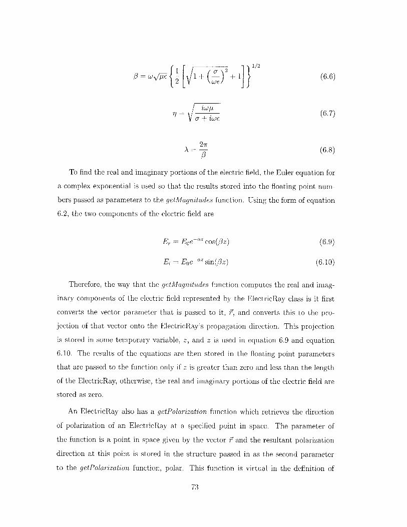
13=: CA)5 - 1 + - + 11 (66)2 (6
rI (6.7)
2irA = (6.8)
To find the real and imaginary portions of the electric field, the Euler equation for
a complex exponential is used so that the results stored into the floating point num-
bers passed as parameters to the getMagnitudes function. Using the form of equation
6.2, the two components of the electric field are
E, = EOe"z cos(3z) (6.9)
Ei = Eoe" sin(z) (6.10)
Therefore, the way that the getMagnitudes function computes the real and imag-
inary components of the electric field represented by the ElectricRay class is it first
converts the vector parameter that is passed to it, F, and converts this to the pro-
jection of that vector onto the ElectricRay's propagation direction. This projection
is stored in some temporary variable, z, and z is used in equation 6.9 and equation
6.10. The results of the equations are then stored in the floating point parameters
that are passed to the function only if z is greater than zero and less than the length
of the ElectricRay, otherwise, the real and imaginary portions of the electric field are
stored as zero.
An ElectricRay also has a getPolarization function which retrieves the direction
of polarization of an ElectricRay at a specified point in space. The parameter of
the function is a point in space given by the vector IF and the resultant polarization
direction at this point is stored in the structure passed in as the second parameter
to the getPolarization function, polar. This function is virtual in the definition of
73

ElectricRay as there are different polarization types for an electric field, circular
or linear. Currently, only a linear polarized ElectricRay known as a LinearRay is
implemented. A LinearRay stores the same polarization direction in the parameter
polar no matter point in space is passed to the function as the parameter, E.
Another method that an ElectricRay has is the getSpreadingLoss function. This
function takes no parameters and returns the amount of spreading loss in dB of the
ElectricRay based on how far the ray has traveled. The equation used to compute
the spreading loss, LD, in dB is given below
LD = -20 log 47D (6.11)
where D is the distance traveled from the radiating origin and A is the wavelength
of the ElectricRay [7]. Since the spreading loss is a loss of power, its result is always
negative. Given these functions and parameters, a ray tracing algorithm may use the
ElectricRay class to model the effects of an electric field.
6.2.2 EMRayTracing Algorithm
The ElectricRay class laid the ground work for the rest of the ray tracing algorithm
by allowing a simple model of an electric field plane wave. The EMRayTracing class
is an EMAlgorithm that implements the ray tracing derivative algorithm.
The idea of ray tracing is nothing new in computer science. At first, ray tracing
was strictly a technique used for image synthesis in computer graphics. Light rays
would eminate from the scene's camera and be cast through each pixel on the screen
and the color of that pixel determined by the ray casting. The concept can be carried
over into other fields besides computer graphics however. Since the frequency used in
UHF RFID is fairly high, this allows for the radio propagation process to be modelled
as rays [21].
The computation function for the EMRayTracing algorithm, like all computation
functions, is passed a collection of Antennas, a collection of Reflectors, and a progress
dialog. The algorithm starts by looping over every Antenna object. For each Antenna,
74

so that each Antenna is treated as an independent radiator, the algorithm retrieves
the location of the different voxel grid vertices, clears the electric and magnetic fields
stored at that vertex and casts an ElectricRay from center of the Antenna towards
that point in space. Although the ElectricRay may be cast in the direction of a
particular vertex in the voxel grid, it will not always reach that destination.
When an ElectricRay is initially cast, it starts with a distance traveled of zero, it
travels in air (as opposed to another medium), and has a specific starting amplitude
based on the type of antenna that is radiating it. Each ray starts with an initial ampli-
tude that is some constant, EFCC. This constant is then multiplied by the directivity
of the Antenna object for the given direction in which the ElectricRay is traveling.
This new scaled constant is then set to be the ElectricRay's initial amplitude, E0 .
The ElectricRay is then begins its casting towards its original destination using the
CastRay method which takes an Antenna and a LinearRay as parameters, a collection
of Reflector objects as a third parameter, and finally takes a integer recursion level
as a fourth parameter. Since a circularly polarized ray may be constructed using two
offset linearly polarized ray, the CastRay method takes a linearly polarized ray as a
parameter instead of a general ElectricRay.
The CastRay function is a general function that casts an already constructed
LinearRay and is the heart of the EMRayTracing algorithm's computation function.
When an LinearRay is cast, a ray-sphere intersection is computed with between the
ray and a maximum bounding sphere of each Reflector. Since a ray-sphere intersec-
tion is easily computed, as it takes roughly six multiplication instructions to compute
the intersection point, this intersection test finds out quickly if a ray is close to inter-
secting with a Reflector [5]. If the ray-sphere intersection results in an intersection,
a more accurate intersection function is used as a generic ray intersection method is
called on the Reflector itself. If the ray intersects with the Reflector, then the time
to intersect, t is then stored into a temporary variable if it is the smallest time to
intersect over all the Reflectors tested so far. The time to intersect, t, is defined as
the point of intersection of the ray can be calculated by the following equation:
75

P 0 + t(O)(.2
where -is the point of intersection, 0 is the ray's origin, t is the intersection time,
and ? is a unit vector in the direction of the ray's propagation direction.
After all the intersection tests are calculated over all the Reflector objects, three
temporary variables have updated values. The first variable, tint, is the minimum
time to intersect the closest Reflector object. A boolean variable, intersect indicates
if the ray does intersect and Reflector object. Finally, a temporary Reflector object,
mediahit, holds the Reflector object that the ray intersects with first, if any. If the
ray does not intersect a Reflector, the time to intersect is longer than the ray's length,
the time to intersect is less than zero, or the current recursion depth of the castRay
function call exceeds a threshold, then the ray is computationally finished. When a ray
is computationally finished, the ElectricRay affects the electric and magnetic fields at
the point of its destination. First, the real and imaginary portions of the electric field
of the ElectricRay at the ray's destination are retrieved from the ray and stored into
variables, Er and Ei respectively. The polarization of the ray is also computed at the
ray's destination and stored in a vector, and its magnetic polarization is stored in
a vector, h. Therefore, the electric field caused by the Electric Ray at its destination
point is given by equation 6.2 and the magnetic field can be calculated using equation
6.3. Each of these fields however is then scaled by the spreading loss of the ray at
it's destination; the spreading loss is easily computed using the getSpreadingLoss
function. The electric and magnetic fields caused by the ElectricRay are then added
to the electric and magnetic fields which are already stored at the ray's destination.
If the ray does intersect with an Reflector and the other criteria for the ray being
computationally finished are not met, then the ray does intersect the Reflector and
more computation is necessary. When an ElectricRay intersects with a Reflector
object, two new ElectricRays are constructed due to the fact that when an electric
field plane wave hits a boundary between two different media, a portion of the wave
is reflected back from the media boundary while the rest of the wave is transmitted
76

Normal
Incident ReflectedMV ray
Figure 6-1: Incident Wave Reflecting Off of Reflector Surface
through the boundary and into the different medium. The two newly constructed
ElectricRays represent the reflected and transmitted portions of the wave after it
impinges upon a boundary between two different media. How these new rays are
constructed is discussed below.
To construct the reflected portion of the wave, the first step is to compute the
ray's origin and destination. The origin of the reflected wave is the intersection point
between the original ray and the Reflector object, mediahit, which can be computed
using equation 6.12. Computing the reflected ray's destination is a little trickier.
When an electromagnetic wave impinges upon a boundary between two different
media, the reflected portion of the wave is reflected back at an angle which is equal to
the wave's incident angle with respect to the normal vector of the reflective surface.
The angle of incidence, 6, is equal in magnitude to the angle of reflection, 0,. The
geometry of the incident and reflected waves can be seen in Figure 6-1 [10].
Once the angle of reflection is known, then the reflected ray's new destination
may be computed. Using equation 6.12 and having the parameter t being equal to
the original ray's length minus the original ray's distance to intersect, tint and having
the ray's direction being the newly computed reflection direction, the reflected ray's
new destination is computed. The length of the reflected ray is equal to the length of
untraversed portion of the original ray's length, therefore the length of the reflected
77

ray and the length that the original ray had to travel to intersect with the Reflector
sum to the total length of the original ray.
The next steps in constructing the reflected ray are to set the medium in which
it is traveling, to set its initial amplitude, and to set its polarization directions. The
reflected ray travels in the same medium that the original ray was traveling in, so
the medium is simply retrieved from the original ray and then that parameter is set
for the reflected ray. The amplitude of the initial ray at the intersection point may
be calculated by using the getMagnitudes function with the total amplitude, E(i),
being the magnitude of the two dimensional complex vector with components given
by the real and imaginary components which were calculated using the getMagni-
tudes function. But the initial amplitude of the reflected ray is not the same as the
amplitude of the original ray at the intersection point. Since the original ray is split
into two different rays, the amplitude of the original ray is then "spread across" the
reflected and transmitted rays and not necessarily equally. The reflected ray's initial
amplitude, EO, at the point of intersection is a scaled version of the original ray's
amplitude at the intersection point where the scaling factor is the reflection coeffi-
cient, R. The reflection coefficient is based on the intrinsic impedances of the two
media, ql and 'q2 respectively and -1 < R < 1. The reflection coefficient may be
calculated using the equation below.
R = 'q2 - *71 (6.13)772 + "71
The subscripts denote the two different media with a subscript of 1 indicating the
media in which the ray is original traveling and the subscript of 2 denotes the media in
which the original ray is impinging upon. Using these equations, the initial amplitude
of the reflected ray, EO, = REi(p) where -is the point of intersection between the
original ray and the intersected Reflector object, mediahit. If R < 0 then the the
polarization of the reflected ray is then the opposite of the polarization of the ordinal
ray at the point of intersection, but if R > 0, then the polarization of the reflected
ray is the same as the polarization of the reflected ray at the intersection point.
78

Figure 6-2: Incident Wave Transmitting Through Reflector Surface
The final parameter to be set is the distance traveled of the ray; the reflected ray is
said to have traveled the original ray's distance traveled plus the intersection distance
between the original ray and the Reflector in which it intersects. Now the reflected ray
has a polarization, an initial amplitude, a media in which it is traveling in, a distance
traveled, an origin, and a destination and with those parameters, the reflected ray is
almost ready to be cast [10].
The transmitted ray, or the ray that is transmitted through the boundary of
the two media is constructed much like the previously discussed reflected ray. The
reflected and transmitted differ in the media in which they are traveling, their des-
tination point, their polarizations, and their initial amplitudes; all other parameters
remain the same. To find the destination point of the transmitted ray, the direction
in which the transmitted ray travels must first be found. Using Snell's law, which is
dervied from phase matching conditions, one has a relationship between the incoming
ray's angle of incidence, 9i and the transmitted ray's angle of transmission, 9 t. The
geometric relationship between the two angles may be seen in Figure 6-2.
79

Snell's law states that the sine of the angle of incidence and angle of transmission
are proportional, but that there does not have to be an angle of transmission; the
equation relationship is given below.
ni sin(0i) = nt sin(0t) (6.14)
Where ni and nit are the indices of refraction at a given frequency of operation for the
media in which the incident ray travels in and the media in which the transmitted
ray travels in, respectively. Finding the media in which the incident ray travels in
is a matter of retrieving that information from the original ElectricRay. To find the
transmitted media is a little trickier. First, one must find out if the original ray is
entering or leaving the Reflector object in which it intersects. If it is entering the
Reflector, the the transmitted media is equal to the Reflector object, mediahit, if the
ray is leaving the Reflector, then the transmitted media is assumed to be air. For now,
the algorithm assumes that Reflector objects cannot overlap, so having overlapping
Reflectors may produce incorrect results.
Now that the proper transmitted media has been found, the transmitted ray is
set to be traveling in that media and the transmission direction, Ot may be calculated
if one exists. If the angle of incidence is beyond the critical angle, 0c, then there is no
transmission direction and the transmitted ray has the same origin and destination
point. The destination point of the transmitted ray is then calculated from the
transmission direction in the same manner as the reflected ray's destination point was
calculated from the reflection direction. The transmitted ray's length is the original
ray's length minus the length from the original ray's origin and the intersection point.
The last bit of information to calculated is the transmitted ray's initial ampli-
tude, EOt. Much like the reflected ray, the transmitted ray's initial amplitude is
proportional to the original ElectricRay's amplitude at the intersection point, so that
EOt = TE,(p) where P is the point of intersection between the original ray and the
intersected Reflector object, mediahit, and T is known as the transmission coefficient.
The transmission coefficient can be calculated using the equation below with Tit being
80

the intrinsic impedance of the transmitted media and 77 being the intrinsic impedance
of the incident media.
T = 2Tt (6.15)77t + Tli
Note that the transmission coefficient can never have a negative value, therefore, the
polarization of the transmitted ray always has the same polarization of the original
ray [10].
Once the reflected and transmitted rays are constructed, then if their magnitudes
are beyond a certain cutoff threshold, then they are recursively cast using the same
CastRay function with an increased recursion level parameter. The magnitude cutoff
is used to save computation. At a certain magnitude level, the contribution to the
any electric field that a given ElectricRay may add is insignificant and not worth the
extra computation for such a small contribution to the overall power level. Once the
newly constructed rays are recursively cast, then original ray is deleted.
All of the above is done for each single Antenna object, the next step is to then
use superposition to sum the power for each independent radiator to find the total
power at a given point in space. After the algorithm has completely run, an Antenna
object, at each vertex of its voxel grid, contains the total electric and magnetic fields
at that location in space caused by all of the radiating agents, not just the fields
caused by each individual radiator.
81

82

Chapter 7
Analysis of the Simulation Engine
The Simulation Engine of RFID Vis consists of a well defined and implemented class
hierarchy which allows for new electromagnetic simulation algorithms to be imple-
mented as well as an implemented simulation algorithm based on ray tracing concepts.
The structure and overall usefulness of the electromagnetics engine's structure is de-
scribed in section 6, this section analyzes in detail the complexity and speed of the
currently implemented electromagnetics simulation algorithms.
7.1 Analysis of EMRayTracing Algorithm
The EMRayTracing algorithm, as previously described, consists of casting "rays"
through each vertex in a collection of vertices for each Antenna object and tracing the
path of these "rays" as they are radiated from the Antenna. While a ray is traveling
from its origin to its destination, the ray may interact with a number of Relfector
objects and then spawn additional rays which are cast. Therefore, the algorithm's
behavior is changed with the number of Reflectors in the RFID environment as well
as the number of vertices in an Antenna's voxel grid that is defined over a particular
region of space. This section describes the EMRayTracing algorithm's complexity,
speed, and how the number of Reflector objects and voxel vertices affect the speed of
the algorithm on varying computer hardware.
83
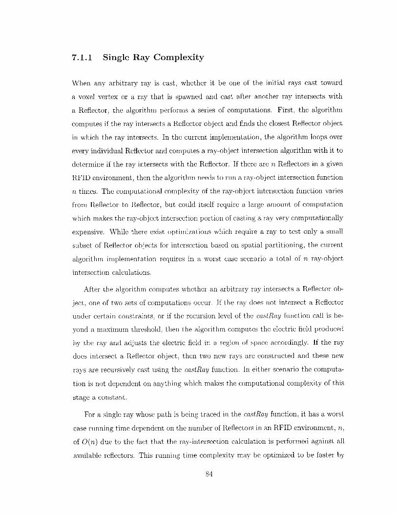
7.1.1 Single Ray Complexity
When any arbitrary ray is cast, whether it be one of the initial rays cast toward
a voxel vertex or a ray that is spawned and cast after another ray intersects with
a Reflector, the algorithm performs a series of computations. First, the algorithm
computes if the ray intersects a Reflector object and finds the closest Reflector object
in which the ray intersects. In the current implementation, the algorithm loops over
every individual Reflector and computes a ray-object intersection algorithm with it to
determine if the ray intersects with the Reflector. If there are n Reflectors in a given
RFID environment, then the algorithm needs to run a ray-object intersection function
n times. The computational complexity of the ray-object intersection function varies
from Reflector to Reflector, but could itself require a large amount of computation
which makes the ray-object intersection portion of casting a ray very computationally
expensive. While there exist optimizations which require a ray to test only a small
subset of Reflector objects for intersection based on spatial partitioning, the current
algorithm implementation requires in a worst case scenario a total of n ray-object
intersection calculations.
After the algorithm computes whether an arbitrary ray intersects a Reflector ob-
ject, one of two sets of computations occur. If the ray does not intersect a Reflector
under certain constraints, or if the recursion level of the castRay function call is be-
yond a maximum threshold, then the algorithm computes the electric field produced
by the ray and adjusts the electric field in a region of space accordingly. If the ray
does intersect a Reflector object, then two new rays are constructed and these new
rays are recursively cast using the castRay function. In either scenario the computa-
tion is not dependent on anything which makes the computational complexity of this
stage a constant.
For a single ray whose path is being traced in the castRay function, it has a worst
case running time dependent on the number of Reflectors in an RFID environment, n,
of O(n) due to the fact that the ray-intersection calculation is performed against all
available reflectors. This running time complexity may be optimized to be faster by
84
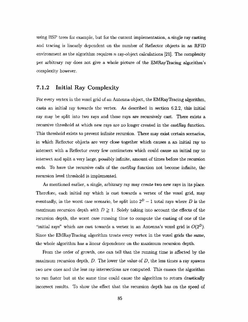
using BSP trees for example, but for the current implementation, a single ray casting
and tracing is linearly dependent on the number of Reflector objects in an RFID
environment as the algorithm requires n ray-object calculations [21]. The complexity
per arbitrary ray does not give a whole picture of the EMRayTracing algorithm's
complexity however.
7.1.2 Initial Ray Complexity
For every vertex in the voxel grid of an Antenna object, the EMRayTracing algorithm,
casts an initial ray towards the vertex. As described in section 6.2.2, this initial
ray may be split into two rays and these rays are recursively cast. There exists a
recursive threshold at which new rays are no longer created in the castRay function.
This threshold exists to prevent infinite recursion. There may exist certain scenarios,
in which Reflector objects are very close together which causes a an initial ray to
intersect with a Reflector every few centimeters which could cause an initial ray to
intersect and split a very large, possibly infinite, amount of times before the recursion
ends. To have the recursive calls of the castRay function not become infinite, the
recursion level threshold is implemented.
As mentioned earlier, a single, arbitrary ray may create two new rays in its place.
Therefore, each initial ray which is cast towards a vertex of the voxel grid, may
eventually, in the worst case scenario, be split into 2D - 1 total rays where D is the
maximum recursion depth with D > 1. Solely taking into account the effects of the
recursion depth, the worst case running time to compute the casting of one of the
"initial rays" which are cast towards a vertex in an Antenna's voxel grid is 0(2D).
Since the EMRayTracing algorithm treats every vertex in the voxel grids the same,
the whole algorithm has a linear dependence on the maximum recursion depth.
From the order of growth, one can tell that the running time is affected by the
maximum recursion depth, D. The lower the value of D, the less times a ray spawns
two new ones and the less ray intersections are computed. This causes the algorithm
to run faster but at the same time could cause the algorithm to return drastically
incorrect results. To show the effect that the recursion depth has on the speed of
85

Figure 7-1: Example of a Complex RFID Environment
simulation, a test RFID environment was developed which contains a single Antenna
object in patch mode, with eight small MaterialBoxes placed in a pallet like config-
uration so that the boxes are very close together. A screenshot of the environment
can be seen in Figure 7-1.
With the MaterialBoxes being close together and close to the Antenna, there
is assumed to be lots of reflections between the boxes and therefore there may exist
plenty of recursive calls of the castRay function. With many recursive calls, the effects
that changes to the maximum recursive depth may be seen more easily. Results of
changing the maximum recursion depth are discussed below.
86
Simulation Time Dependence on Maximum Recursion Depth for a Complex Environment
50 100 150 200Maximum Recursion Depth
Figure 7-2: Simulation Time Depedence on Maximum Recursion Depth
87
25
20 1-
U)
00a)
E
0Cz
E
15
10[
5
00 250

A graph depicting the simulation run time's depedence on the recursion depth can
be seen in Figure 7-2. The simulation data is graphed along side a scaled function of
2 D to show that the function 2D performs worse than the simulation and is the worst
case scenario running time. Part of the reason why the simulation performs better and
the simulations times do not double as the maximum recursion depth increases by one.
This is because, not all rays in the scene will be intersecting a Reflector, therefore,
some rays will not be effected by the increase in maximum recursions depth, only a
fraction of them will and other computation will remain constant. The effect of the
maximum recursion depth also begins to lessen as D increases because the recursively
split rays eventually fall below the amplitude cutoff threshold for recasting a ray, so
then the rays are never split to begin with.
7.1.3 Resolution Complexity
Most of the algorithm parameters which have been analyzed in the preceding sections
are parameters which are encoded into the source code as constants. The values for
the constants were decided on by testing different environments to see which values
have a good balance between performance and results. There are parameters that
affect the EMRayTracing algorithm, or any EMAlgorithm for that matter, which can
be altered and controlled by the user of RFID Vis, the simulation resolution, which
can be altered through the RunSimulationDialog, and the width/height/depth of the
Antennae's field.
Strictly speaking, these parameters do not affect EMAlgorithms, they affect all
the Antenna objects in a scene by changing the number of vertices in the Antenna's
voxel grid. As previously described, the job of an EMAlgorithm is to compute the
electric and magnetic fields at each vertex of each Antenna's voxel grid. Therefore,
changing these parameters changes the total number of vertices in an Antenna's voxel
grid which could cost the algorithm more computation time.
The EMRayTracing algorithm, casts an "initial ray" towards each vertex in an
Antenna's voxel grid for each Antenna, so the more vertices, the more rays need
to be cast. The total number of vertices for an Antenna's voxel grid is given by
88

Pattern Width Pattern Height Pattern Depth Simulation Time(seconds)5 5 5 1.510 5 5 2.812515 5 5 4.1255 10 5 2.81255 15 5 4.1255 5 10 2.8755 5 15 4.125
Table 7.1: Effects of the Antenna Pattern Dimension on Simulation Times
(1 * r + 1)(w * r + 1)(d * r + 1), where 1 is the Antenna's field length, w is the field
width, d is the field depth, and r is the field resolution which may vary between
simulation to simulation. With all other parameters in the algorithm kept constant,
the ray tracing algorithm has a worst case running time dependence of O(l*w*d*r 3).
The actual dependencies should be better than the worst case scenario since most rays
will not be recursively cast to the maximum recursion depth.
The algorithm has a linear dependence on each of the Antenna's field dimensions
and a cubic dependence on the field resolution (the number of calculation points
per meter). To show the effects that changing these parameters has on the speed
of a simulation, a few tests were run. Each test used an RFID environment which
has become standard for most of the tests that were used to test the simulation,
the environment consists solely of an Antenna of a patch type. To see the effects
of the different parameters, the parameters were changed one at a time and a new
simulation was run with the new parameter settings. The running time of each of the
simulations were recorded. The data of the tests can be seen in Table 7.1 and Table
7.2. For the tests in which Antenna pattern dimensions were changed, a simulation
resolution of 5 was used, one dimension was altered at a time while the other two
dimensions remained constant. For the test noting the changes caused by the change
in resolution, all the pattern dimensions were 5 meters.
Graphs which plot the simulation times with respect to the different changes of
pattern dimensions and simulation resolution can be seen in Figure 7-3 and Figure 7-
4. The dependence on each pattern dimension can be seen to be linear while the time
89

Simulation Resolution Simulation Time(seconds)5 1.510 11.437515 39.687520 88.7525 152.187530 234.187535 418.1875
Table 7.2: Effects of the Simulation Resolution on Simulation Times
dependence on the simulation resolution is close to cubic in nature. These results fit
well with the calculated running time complexities for the algorithm. The depedence
on the simulation resolution is also graphed with a scaled cubic function to show
the cubic relation of the dependence on the simulation resolution. The simulated
data performs slightly better than the cubic function becomes some rays require less
calculations as their amplitudes may be too small to consder certain operations on.
Overall, the data matches the predicted worse case scenario behavior.
7.1.4 Real-time Analysis
The previous portions of this section discuss the overall running time of the EM-
RayTracing algorithm based on certain parameters of the algorithm and how the
parameters affect the speed of the simulation. While the sections discuss the param-
eters' effects individually, the algorithm is too complex to mathematically describe in
full detail as there are many conditional situations involved. While the algorithm is
complex and cannot truly be written in a formulaic style, the overall running time of
particular simulations and overall performance and running speed of RFID Vis can
be measured accurately.
One of the main features of RFID Vis is the quick production of results to always
give the user some active feedback as to the behavior of the electromagnetic power
in the environment. A constant stream of feedback allows the user's actions to be
guided instead of having the user blindly altering the environment without knowing
how the alterations will affect the electromagnetic power.
90

4.5 1Width
- - -HeightDepth
4-
3.5-U)
0
0
co
ES2.5-
2
1.55 6 7 8 9 10 11 12 13 14 15
Antenna Pattern Dimension (meters)
Figure 7-3: Graph of Simulation Times Based on a Single Pattern Dimension
91

Simulation Time Dependence on Simulation Resolution
_ imuation ata0.012 x3
- .A
- -
- -
F -
F/
10 15 20 25 30 35Simulation Resolution (calculations per meter)
Figure 7-4: Graph of Simulation Times Based on Simulation Resolution
92
600
500
-400
0U)
E300
0
Ec7 U)
100
05
200 u

Real-Time Simulation Resolution Average FPS1 8.962 33 1.15
Table 7.3: Average Real-time FPS While Using a Complex RFID Environment
Having a decent real-time simulation is a key component of RFID Vis therefore a
few of the algorithm's parameters must be tweaked so that the real-time simulation
runs sufficiently quick for moderate size environments on average computer systems.
To find a good set of parameters for the real-time simulation, a moderately complex
RFID environment was used to test the speed of RFID Vis when using the real-time
simulation. A moderately complex RFID environment consists of a single Antenna
and a moderate amount of MaterialBox objects (around 8); an example can be seen
in Figure 7-1.
In this environment, the goal was, when running the real-time simulation almost
constantly, to have RFID Vis be running at roughly 3 FPS on an average computer
system.
To test the speed of the real-time simulation on different systems, the moderately
complex environment was loaded into RFID Vis and the real-time simulation was
set to always be running. The average FPS of RFID Vis was recorded for a few
different systems as were the different parameters used by RFID Vis during the tests.
The antenna pattern dimensions used during the test were 5 meters in each primary
direction. The data from the tests may be seen in Table 7.3. One may note that for
the computer used, only a resolution of 1 would remotely acheive close to the desired
results. Due to the complexity of the scene, the real-time simulation runs a bit slower
than it usually does. Optimizing the algorithm may speed up the real-time simulation
in future versions to be closer to real-time.
After some thought, it was decided that most of the parameters for the real-time
simulation may be set to a set of generic, well tested values, but the simulation
resolution for the real-time simulation needs to be alterable by the user somewhat.
Due to the fact that the real-time algorithm has a cubic dependence on the simulation
93

resolution, this one parameter has the largest single effect on the running time of
the real-time simulation. Giving the user free reign over the value of the simulation
resolution may result in having the resolution be too high and RFID Vis being caught
in an immense set of calculations, but the user needs to have some control over the
value of the resolution because if the user is using a rather low end piece of hardware,
the default resolution for the real-time simulation may be too high for the hardware
to handle at a decent speed.
The data seen in Table notes that for a high end or average system, that a res-
olution of two calculations per meter seems to be sufficiently low to produce quick
enough results for a moderately complex environment in close to real-time, but if
the user is using a low end system or if the environment becomes more complex,
this default real-time resolution may be too high to produce quick enough results to
be real-time. The real-time resolution may also be too low, in case the user has a
high end system and would like better looking results. In these situations, it may
be helpful to have the resolution for the real-time simulation be set at an alternative
value than the default value. Therefore, the resolution for the real-time simulation is
adjustable to be either 1 (the lowest possible), 2, or 3 calculations per meter. This
allows the user more control, allows the simulation to be real-time for a number of
different scenarios as the user is able to allow for faster, although less accurate and
harsher looking results.
7.1.5 Analysis of Produced Results
Most of this sections has been discussing the speed and complexity of the EMRay-
Tracing algorithm, but there has been little discussion of the accuracy of the electro-
magnetic results produced by the algorithm. Even if the algorithm ran with blazing
speed, if the results produced are in no way accurate, then the algorithm is useless
and the speed of the algorithm is inconsequential. This subsection describes results
produced by the algorithm and questions their validity.
There was an inherent difficulty in testing the validity of the algorithm in com-
parison to a real RFID set up for a number of reasons. First of all, the model used
94

for an Antenna object allows the Antenna to be of either an isotropic or patch type.
In reality, most of the antennae used are not patch antennae, but have very complex
radiation patterns which are not easily written in as a formula. Because of this, en-
vironments created in RFID Vis can never mirror real environments which makes it
difficult to compare results of RFID Vis to real results. Also, it is very difficult to
measure the electromagnetic power at a particular point in space as doing so requires
special tools which I cannot acquire.
With mismatched models and difficulties measuring exact power in real environ-
ments, testing the validity of algorithm results was done in a round-about fashion.
While I would have liked for the simulation to be as accurate as possible, it was
deemed acceptable to have the algorithms produce accurate qualitative results that
may only be accurate to within an order of magnitude or so. Since RFID Vis was
designed as a predictive tool which predicts electromagnetic behavior as opposed to
a tool to show exact solutions, having the EMRayTracing algorithm be qualitatively
accurate as opposed to wholly quantitatively accurate was what was tested to check
the validity of the algorithm.
To test the qualitative accuracy of the algorithm, a few tests were run to see if
the algorithm predicts certain behavior that was already proved to occur in reality.
The first test was simply seeing if more metallic objects reflect back more power. To
test this, a MaterialBox of default size was set to be filled with air with an Antenna
object radiated power on it. The box was then changed to be filled with water and
aluminum and, using a Tag object to take power measurements within RFID Vis, the
electromagnetic power at the surface of the box is measured and compared between
the three cases; the results of the test can be seen in Table 7.4. The more "metallic"
the object, the more power is reflected back. A box filled with Air did not cause a
reflection, so the power at the surface of the box filled with air was used as a basis
for comparison. When the box was filled with water, some power was reflected, but
when it was filled with a highly reflective material such as aluminum, it can be seen
that RFID Vis simulated that even more power would be reflected which is the case
in reality.
95

Material Microwatts at MaterialBox SurfaceAir 15.890
Water 208.707Aluminum 341.015
Table 7.4: Simulated Reflective Power Differences Between Materials
The next test performed tested if the algorithm was capable of producing standing
waves. A standing wave is produced when a plane wave reflects off of a perfect
conductor at normal incidence. The reflected wave destructively interferes with the
incoming wave creating null spots at certain locations in space. While there is no
perfect conductor medium available to fill a MaterialBox with, aluminum is close to
it. So, the test used to check for a standing wave is to have an Antenna object of a
patch type radiating on a very large MaterialBox that is filled with aluminum. The
large size of the MaterialBox is used to increase the chance of a plane wave intersecting
at a close to normal angle of incidence, but since the box is filled with aluminum and
the incident angle is not exactly 90 degrees, there are no exact null spots with no
power, but point of very low power in comparison to points around it. A very high
resolution simulation is then run to see in more detail the exact workings of the
electromagnetic power. A screenshot of the produces inteferance waves can be seen
in Figure 7-5. One can note the periodic regions of low power in the screenshot which
is indicative of standing wave type behavior which shows that the EMRayTracing
algorithm is capable of of calculating interference between waves.
One final test that was run to test the validity of the EMRayTracing algorithm
was developed to show that the algorithm can mimic a peculiar behavior of water.
When an plane wave is incident upon water, a portion of the wave is transmitted
into the water and a portion is reflected back. After the transmitted portion travels
through the water, the wave is then incident on another boundary between water and
air at the back of the container of water. Again, a portion of this wave is reflected
and transmitted through the boundary. It turns out, as to be expected, the available
power at the back of the container of water is dependent on the thickness of the water
(how much water the wave traveled through), t. Varying the value of t yields very
96
Figure 7-5: Simulated Destructive Interference
interesting results. One notes that, somewhat counter-intuitively, the power measured
at the back of the water varies periodically with the thickness t although their does
exist a dampening envelope of the crests of the power which is to be expected.
To test for this behavior in RFID Vis, an environment was created which contained
an Antenna object of a patch type radiating on a MaterialBox full of water. The
Antenna is placed close to the box and at an angle close to 90 degrees. A Tag object
is placed on the back of the box to measure the power there. The thickness of the
water (along the same axis that the Antenna is radiating towards) was then altered
by 2 centimeters. The thickness started at a relatively low value and increased in
small increments. The power at the back of the MaterialBox were recorded at each
value of the thickness, t, for simulations at a resolution of 10 calculations per meters.
The data measured can be seen in Figure 7-6.
Notice how the measured power is periodic as a function of t; much like it is
in reality, but is a little off. In reality, the power is periodic at roughly every half
97

wavelength, which in this case would be around 16 centimeters [1]. The graph of
the data does not match eactly the behavior of reality due to a few small reasons.
The simulation, as previously mentioned, calculates the power at a given voxel vertex
and the powered measured at a point in space is the power at the closest voxel
vertex. Therefore, if a point is not exactly on a voxel vertex, the power measured
will be close, but not exactly what is measured at that given point. This may cause
somewhat inconsistent data in the graph that creates amplitudes that are too high
or too low; the spikes between the larger amplitudes may be due to the fact that the
power actually being read may be from a point not quite on the surface of the box.
The box is of finite width as well which may cause reflections off of the side which may
cause the spikes in the graph. Also, the test was run every 2 centimeteres, where as
some of the peaks in the power may not have been at the points which were measured,
this causes some of the maxima to not quite fit the decay envelope. A finer resolution
simulation and more data points would solve these problems, but would have made
the gathering of this data take days or months as opposed to hours. Indiscrepancies
also exist due to the model used in the simulation algorithm. The graphed results
do show the general decaying periodic behavior which is what the test was set out to
prove the algorithm was capable of. This test demonstrated that the algorithm was
able to, without any special hard coding or special scenarios, able to mimic a realistic
behavior which vouches for the validity of the algorithm as a whole.
7.1.6 Summary of EMRayTracing Analysis
Overall, the currently implemented EMRayTracing algorithm, which is also the cur-
rent real-time algorithm used in RFID Vis, is a very complex algorithm, but is easy to
implement and can produce decent results in real-time. The algorithm is also capable
of making very accurate, great looking results through use of higher resolution sim-
ulations. The results produced by the algorithm accurately portray electromagnetic
behavior to within an order of magnitude or so.
98

140
120
100-
00E
7 80-
0
0'-40-
20
010 10 20 30 40 50 60 70
Water Thickness (cm)
Figure 7-6: Simulated Electromagnetic Power Propagating Through Water
99

The algorithm could become faster with some more optimizations as it is not the
most scalable of algorithms in the current implementation. There are many ways
to optimize the algorithm, one of which deals with spatial optimization and can
use a BSP tree to separate a scene into many smaller subscenes[20]. These spatial
optimizations allow the algorithm to not have to compute n ray-object intersections,
but some smaller number than that.
The algorithm also struggles with objects that are very close together as their
ray-object intersection times are very similar and a problem can arise with the pre-
cision of floating point numbers and these very small intersection times. Overall, the
algorithm works well, even as a real-time algorithm but struggles in a few cases and
the performance degrades quickly when more Reflectors are added to an environment.
100

Chapter 8
Conclusions
This chapter presents the conclusions that I have made about RFID Vis in general as
well as its implementation and other aspects of RFID Vis. Future extensions of the
current implementation and other improvements are also discussed.
8.1 RFID Vis Conclusions
The main purpose in creating RFID Vis, as discussed in Section 1.3, was to create the
underlying modular structure for a tool which would allow users of UHF RFID tech-
nology to increase their intuition and understanding of electromagnetics in a quick
and intuitive manner. To accomplish this task, RFID Vis needs to produce accurate
results quickly for very specific environments while being easy to use. Overall, RFID
Vis accomplishes this task. While it is not an end all solution to every RFID problem,
it accomplishes the tasks it is created to handle. RFID Vis allows users to create en-
vironments that resemble pallets in warehouses, computes the electromagnetic power
over given volumes of space within a certain degree of accuracy, computes the results
quickly, presents the data to the user in a graphical manner which makes the results
easier to understand, and is easy to use with a very small learning curve. I am par-
ticularly proud of the visualization of the electromagnetic power as the transparent
effect and the coloring scheme blend well and are easy to understand.
While RFID Vis accomplishes the tasks for which it was created, it is not without
101

its limitations although these limitations do not encumber the usefulness of RFID Vis
as a whole. One of the major drawbacks of RFID Vis is the fact that the Antenna
object has only a set number of types which do not exactly mimic the antennae used
in real world implementations of UHF RFID environments. The reason for this is the
fact that many of the antennae used in the real world do not have analytic functions
which describe their radiation pattern. It is entirely feasible that, given a general
form for a radiation pattern, if antenna manufacturers provided such equations for
the radiation patterns that RFID Vis would be able to handle any type of antenna
type. Unfortunately, the only radiation patterns available to me in formula form were
for the antenna types given. More may be able to be added quickly, but due to time
restraints, only the two types currently implemented are available.
Another limitation of the current implementation of RFID Vis is that the number
of available objects is somewhat small and the boxes of the material are required
to be rectilinear and filled with homogeneous product instead of an arbitrary shape
and filled with arbitrary product. Having an arbitrary shaped object filled with
arbitrary product is completely within the scope of RFID Vis as the regions of different
products would all be different Reflector objects. The reason that all of the currently
implemented objects are rectilinear is that the meshes for those objects are very simple
to compute. Future work could allow the users to create a new object type that could
read in user defined meshes, as modular design of RFID Vis would easily allow that,
time constraints forced the current implementation to use predefined meshes which
needed to be computationally simplistic in nature.
One last minor limitation is that the currently implemented EMRayTracing algo-
rithm is not optimized as well as it could be, as is discussed in Section 7.1. This causes
the real-time simulations to not perform as well on lower end machines and limits
the algorithm's scalability as more objects are added. This is a minor non-optimality
which can be alleviated with an algorithm tweak, but under the time constraints, a
simplified version of the algorithm was used.
Overall, the currently implemented version of RFID Vis defines and uses a well
constructed hierarchy of objects and data which may be easily extendible for added
102

features in future versions. The current version works well and achieves its goals.
The current version allows users to understand the fundamentals of electromagnetic
behavior at UHF frequencies quickly and easily which helps the user develop intu-
ition about electromagnetic behavior. Future versions may allow users more freedom
when creating specific environments which may allow for more realstic environment
creation. More freedom and flexibility helps develop intuition more quickly and may
provide some real-world solutions to very specific RFID problems. In the end, the cur-
rent implementation of RFID Vis defines a rich structure and idea as well as acheiving
the goals that I set out to accomplish in creating it.
8.2 Future Work
Most of the limitations with the current implementation of RFID Vis are not limi-
tations with it as a whole, but are features that were not implemented in the time
alloted. This section will briefly discuss some features that may be added in future
versions of RFID Vis to increase its power and usefulness to RFID users as a whole.
One feature that may be added in the future is for the user to be able to have
different materials in a box instead of a homogeneous material. Users would possibly
be able to specify a mesh to read in from a file and a file that specifies which parts
of the box contain what materials. This would be useful because, as we know, a
box full of packaged products is never homogeneously filled with the product. A
simple version of this feature would be straightforward to implement as each region
of different material could be considered different Reflector objects and no currently
implemented code would need to be altered. I say a simple version because this feature
would be very difficult to implement with a high level of detail. In all actuality, a box
of products is quite complex to model completely. The outmost box has a set thickness
which may be variable from company to company. Then the box which contains the
individual products has a thickness, or maybe the products are contained in plastic
and cardboard which would complicate things even more as these layers are usually
thin and somewhat negligible. So, having this feature in a full level of detail to try to
103

mimic reality perfectly would be difficult for the programmer of the next version of
RFID Vis and the user because the user would have to specify such small features in
a mesh. Therefore, a simple version of the feature is much easier to implement and
is very feasible in a future version of RFID Vis.
Another set of features to be added deal with optimizations. Using vertex or pixel
shaders to handle most of the volumetric calculations or even most of the algorithm
computations. This frees up CPU cycles and allows for a faster computation time.
The CPU then could be spent doing other work to make the algorithms more complex
or the visualizations to look better, but at the very least, hardware accelerating RFID
Vis would lead to an increase in performance. Also, when fetching the amount of
power at a given point in space, tri-linear interpolation could be used instead of
direct sampling to achieve a more accurate result of the power at the point if it does
not directly lie on the vertex of a given Antenna's voxel grid. Some space partioning
could be used in the ray tracing algorithms to speed things up as well. There are
many places where RFID Vis can be more optimized.
Other features which may be added could be the ability for users to specify their
own type of Antenna. As mentioned before, only two types are currently implemented,
but it is feasible to, if given a standard format for the equations to use, that the
radiation pattern of an Antenna can be read in from a file and then used in RFID
Vis. This would allow the Antenna in RFID Vis to be closer to the real antennae which
the users of RFID Vis are using. Unfortunately, this would require knowledge of a
equation which represents the radiation pattern of specific antennae which are usually
either unknown or not supplied by the antennae manufacturers, but the functionality
for it is implemented and this feature is feasible in future versions.
The main work which should be added to RFID Vis is refinement and imple-
mentation of new algorithms. As previously mentioned, the only algorithm currently
implemented in RFID Vis is the EMRayTracing algorithm and this algorithm is un-
optimized. Future work could be done optimizing this algorithm so that the real-
time aspect of RFID Vis is fast even on low end machines. Also, new algorithms
could be implemented since RFID Vis specifies an algorithm class which is easily ex-
104

tended. These new algorithm may take more concepts into consideration beyond first
principles and may produce better results than the ray tracing algorithm currently
implemented. The speed of these algorithms is of no concern as these simulations
will only be available through the RunSimulationDialog and will not be running in
real-time. These new algorithms should be as precise as possible so that better and
better results may be produced.
Other side amounts of work could be to develop a collision detection algorithm
that is generalized so that object may not overlap each other as well as adding some
lighting which would help the users be able to specify environments faster. Of course,
the user interface can be tweaked and refined to add more and more features.
Overall, the amount of features which may be added to RFID Vis are endless
and because RFID Vis has a well designed architecture for both electromagnetic
algorithm implementation and object implementation, most of these features may
be easily added without manipulating any of the existing code base. This is the
underlying beauty of the work I have done in developing RFID Vis and I hope future
versions of it will benefit from my design.
105

106

Appendix A
User Manual for Simulation Tool
A.1 Installation
To install the Graphical Real-time Simulation Tool for Passive UHF RFID Environ-
ments, simply run the supplied installation executable, setup.exe. The simulation
tool requires Windows XP to operate as well Microsoft's DirectX 9.0 or later. The
installation CD should have an installation executable for DirectX 9.0, but the latest
version of DirectX is also downloadable from www.microsoft.com
To run the simulation tool, use the shortcuts installed on the desktop and start
menu, or run the executable, Packing.exe from the directory where the program was
installed.
A.2 Camera Movement
The following section describes the commands for moving the camera around in the
RFID environment. Default key bindings are mentioned, but these keys may be
changed at any time through the Configure Input menu item in the File pulldown
menu.
The camera used in the simulation tool can be rotated about and moved along
two axes at any given movment. When the W key is pressed, the camera moves
forward along its line of sight, the S key moves the camera backward along this same
107

axis. Pressing the A key gives the camera a command to move left, which moves the
camera left on an axis that is perpendicular to the line of sight and perpendicular to
the current "up" of the camera. The move left command can be thought of as "side
stepping" to the left. When given a move right command, initially bound to the D
key is bound to this command, the camera "side steps" to the right. These are the
majority of the commands that affect the camera's position in space.
The viewing angle of the camera can also be adjusted along two separate axes
and by using the arrow keys, the user can adjust the viewing angle. The camera's
viewing angle is bound to a "sphere" and moves as such. If you imagine the camera
at the center of a sphere, then pressing the up and down arrows increases the viewing
angle along the vertical direction. This angle ranges between straight up and straight
down, but cannot exceed either extremity, so the angle is bound to 180 degrees of
rotation.
Pressing the left and right arrows moves the viewing angle horizontally along the
sphere. The effect of rotating along this horizontal plane of the sphere changes with
the vertical viewing angle of the camera. At the very top of a sphere, there is not
much of a horizontal "ring" to move about, so moving the angle horizontally will have
little affect to changing the view of the camera. This is similar to looking at a spot
on the ground straight down and rotating your yourself around it; you'll only still be
seeing the spot. If the veritcal angle is looking exactly forward, then adjusting the
horitzontal angle changes the viewing direction along the circumference of the sphere.
The viewing angle controls are difficult to describe in words, but are very intuitive
and easy to learn when used.
A.3 Coordinate System
The simulation tool uses a cartesian coordinate system for all of its calculations and
renderings. The origin of the coordinate system is located at the center of the top
surface of the floor of the environment. The x and z axes are along the surface of the
floor while the y axis runs perpendicular to the surface. The x axis can be thought
108

of as a "width" axis, while the z axis is a "depth" axis and the y axis is a "height"
axis. The units of the coordinate system are meters.
A.4 Objects
There are four types of objects currently implemented in the simulation tool: An-
tenna, MaterialBoxes, Tags and Floors. With the exception of Floors, each of these
object may be created through the Insert menu. Only one Floor is present in any en-
vironment in the simulation tool. Manipulating the objects is covered in Section A.5,
this section describes the properties of each object. Each object can be deleted (with
the exception of the Floor) by pressing the delete key. When an object is deleted, all
of it's children are deleted as well. So, deleting a box will delete any tags attached to
it.
A.4.1 Antenna Object
An Antenna object represents a reader antenna and is the most complex object of the
simulation tool. Each Antenna, has the electromagnetic power over a specified volume
of space calculated and rendered to the screen. An Antenna may present different
types of antennae with different gains and directivities and the electromagnetic power
that is rendered may be of varying sizes.
The first parameter of an Antenna object is its type. Currently there are two
types of Antennae, isotropic and patch. There may be more types in the future, but
these are the only types available now. An isotropic antenna has a gain of 0 dBI while
the patch has a gain of 6 dBI.
The electromagnetic power of an Antenna is calculated over a rectangular volume
of space. The maximum extent of the volume is given by three parameters, pattern
width, pattern height and pattern depth. If each of the constants has a value of 5
meters, then the power is calculated to a maximum extent of -2.5 meters to 2.5 meters
along the Antenna's horizontal axis. The power is also calculated to a maximum
extent of -2.5 meters to 2.5 meters along the Antenna's vertical axis as well as a
109

maximum extent of 0 to -5 meters along the Antenna's "z axis." One may note that
only the electromagnetic power in the forward facing or "in front of" the Antenna is
calculated. No power outside the given ranges is calculated; the main use of this is
to save calculation speed. If the user only cares about a predefined region of space,
then only the powers for that region should be calculated.
A.4.2 MaterialBox Object
A MaterialBox is a rectangular box that represents a box used to store items that are
normally placed on pallets. The material inside of the material box can be specified
using three electromagnetic constants. These constants may be specified through
some specified dialog boxes or may be read in from a "material database." The
width, length and depth of the boxes may also be altered through use of dialog boxes.
A box is assumed to have the same material at each point contained within its volume.
The "material database" is read in from a specified text file. This file is in the
relative path "db\materials.txt" The materials in this text file must be specified in a
particular format. The format is as follows:
Material Name[return character] (example: Shampoo)
Electric Permittivity constant [return] (example: 2.09e-012)
Magnetic Permeability constant [return] (example: 1.25e-6)
Electrical conductivity constant [return] (example 3e-02)
Notice the return character after the last constant. This is the case if there are
more materials in the file. For the last material in the database, do not insert
a return character after the last constant. The database file should always end
with the last line being the last constant; the cursor should not be able to move down
to a line below the last constant of the last material. An example file can be seen
below (with no actual numerical accuracy for the constants):
Shampoo
110

3e-12
4e-6
0.0
Steak
6e-12
5e-6
3e-02[ENDI
A.4.3 Tag Object
The Tag object represents a very simple model of a passive UHF RFID tag. A Tag
can be inserted onto a box and can move along the faces of that box. The inner
circuitry of a Tag is assumed to need 10 microwatts to "power on." When there is
sufficient power at the Tag's center, the tag lights up and turns yellow to give a visual
indicator that a minimal power threshold is reached. The power seen by the Tag
circuitry is not the same as the RF power available to the Tag. Each Tag is assumed
to have 20% efficiency at converting RF power to usable power. So, any power read
by a Tag is really one fifth of the available RF power at that point.
A.5 Clicking and Dragging
The main way that the user of the simulation tool can interact with individual objects
is through use of the mouse. When an object is clicked, it is dubbed as "selected."
A bracket will pop up to give an indication as to which object is selected and certain
information about the selected item will appear in the lower right of the screen.
Double clicking an object will cause the camera to zoom to that object, the same
effect occurs when its thumbnail that appears in its information window is double
clicked. Right clicking an object opens up its properties dialog in which certain
properties of the object may be altered. Not all object have a properties dialog.
When an object is clicked and dragged, the object invokes its drag command.
111

When an object is dragged, the axes in which it can be dragged are displayed on the
screen. What axes these are and how the object is moved when it is dragged are
defined by the object individually. Having the control button pressed while dragging
invoke an "alternate drag." On the object. For instance, when you drag a box, it's
normal movement is laterally along the surface of the floor, but the alternate drag
moves it vertically along a third axis.
A.6 Running a Simulation
While a nice graphical front end is an integral part of the simulation tool, if incorrect
or incoherant results are produced, then presenting them to the user in an interesting
way is somewhat meaningless. This section will discuss how simulations are run and
how certain aspects of simulations may be altered.
A.6.1 Real-time Simulations
Most of the simulations that are run in the simulation tool are run "behind the
scenes" and run in real-time. This real-time simulation is based on a Ray Tracing
algorithm with a very low "algorithm resolution." This means for every meter is
space, there is a specified number of points spread equally across a meter in which
the power is calculated. The lower this number, the less calculations an algorithm
must compute and the faster the simulation run. So, for a real-time simulation, this
resolution is set relatively low so that results may be produced in a timely manner.
Since different machines run at different speeds, this resolution parameter can be
alternated between three low values through use of the Edit Realtime Parameters
menu item in the Simulate menu.
The real-time simulation is run when objects are moved or properties are changed
in which a simulation must be rerun. Since the user needs some way of knowing the
general effects that certain changes has and these changes may happen frequenlty
(such as when an object is being dragged, it's displacement changes very frequently),
the user needs the results of a simulation in a very fast manner. This is where the
112

real-time simulation is used. Imagine running a simulation that took 15 seconds
every time an object is moved, this would make dragging an object take minutes to
do because each time the displacement is updated, a new simulation must be rerun.
The real-time simulation exists to give users a general idea of how certain changes
affect the power in the environment in a quick manner; if more accurate results are
required, more accurate simulations may be run once objects in the environment are
stationary.
A.6.2 More Accurate Simulations
While the real-time simulation produces decent results quickly, oftentimes once a
specific environment is set to meet users' needs, users may want to run a more accurate
simulation to produce more accurate results than those produced by the real time
simulaton. When the need for a more accurate results than the real-time simulation
are required, the user may run a slightly slower and more approximate algorithm
through the use of the Run Simulation menu item in the Simulate menu.
When clicked, a dialog opens with two initial parameters to chose from: the
simulation resolution and the algorithm selection. The resolution parameter is the
same as described in Section A.6.1 and the algorithm selection parameter allows
the user to select betwen different types of algorithms. At the moment, only one
algorithm, a Ray Tracing derviative, is selectable. Future versions may include many
more algorithms. Depending on the algorithm selected, the dialog may expand and
contain other algorithm specific parameters.
So, the simulations are used as follows. The real-time simulations guide the user
when the environment changes to show the dynamic alterations in power. Once an
environment is situated to the user's desire, a more finely run simulation may be run
to generate more accurate results.
113

114

Bibliography
[1] Constantine A. Balanis. Advanced Engineering Electromagnetics. Wiley, New
York, NY, USA, 1989.
[2] D. Bouche, F. Molinet, and R. Mittra. Asymptotic Methods in Electromagnetics.
Springer, Berlin, Germany, 1997.
[3] Brian Cabral, Nancy Cam, and Jim Foran. Accelerated volume rendering and
tomographic reconstruction using texture mapping hardware. In VVS '94: Pro-
ceedings of the 1994 symposium on Volume visualization, pages 91-98, New York,
NY, USA, 1994. ACM Press.
[4] Roger Crawfis and Nelson Max. Direct Volume Visualization of Three-
Dimensional Vector Fields. In VVS '92: Proceedings of the 1992 workshop on
Volume visualization, pages 55-60, New York, NY, USA, 1992. ACM Press.
[5] Andrew S. Glassner. An Introduction to Ray Tracing. Academic Press, San
Diego, CA, 1989.
[6] Dr. Todd H. Hubing. Survey of Numerical Electromagnetic Modeling Techniques.
Technical Report TR91-1-001.3, University of Missouri-Rolla, Missouri, USA,
1991.
[7] Radio Innovation. How far will my radio transmit?". Web site containing misc.
radio related data. All copyrights belong to Radio Innovation., 2002.
[8] Kazufumi Kaneda, Yoshinori Dobashi, Kazunori Yamamoto, and Hideo Ya-
mashita. Fast Volume Rendering with Adjustable Color Maps. In VVS '96:
115

Proceedings of the 1996 Symposium on Volume Visualization, pages 7-14, New
York, NY, USA, 1996. ACM Press.
[9] Arie E. Kaufman. Volume Visualization. ACM Computer Survey, 28(1):165 -
167, 1996.
[10] Jin Au Kong. Electromagnetic Wave Theory. EMW Press, Cambridge, MA,
USA, 2000.
[11] R. G. Kouyoumjian. Asymptotic High-Frequency Methods. In Proceedings of
the IEEE, volume 53, pages 864-876, August 1965.
[12] Kangsun Lee and Paul A. Fishwick. OOPM/RT: A Multimodeling Methodol-
ogy for Real-time Simulation. ACM Transactions on Modeling and Computer
Simulations, 9(2):141-170, 1999.
[13] Adrian Leu and Min Chen. Direct Rendering Algorithms for Complex Volumetric
Scenes. Technical report, University of Wales Swansea.
[14] Joshua Leven, Jason Corso, Jonathan Cohen, and Subodh Kumar. Interactive
Visualization of Unstructured Grids Using Hierarchical 3D Textures. In VVS
'02: Proceedings of the 2002 Symposium on Volume Visualization, pages 37-44,
New York, NY, USA, 2002. ACM Press.
[15] Steve McConnell. Code Complete: A Practical Handbook of Software Construc-
tion. Microsoft Press, 1993.
[16] Andrew F. Peterson, Scott L. Ray, and Raj Mittra. Computational Methods for
Electromagnetics. IEEE Press, 1998.
[17] Rao, Glisson, and Wilson. Electromagnetic Scattering by Surfaces of Arbitrary
Shape. IEEE Transmission, Antennas and Propagation, AP-30(3):409-418, May
1982.
116

[18] Takafumi Saito. Real-time Previewing for Volume Visualization. In VVS '94:
Proceedings of the 1994 Symposium on Volume Visualization, pages 99-106, New
York, NY, USA, 1994. ACM Press.
[19] Sandy Sefi. Ray Tracing Tools for High Frequency Electromagnetics Simulations.
Master's thesis, Royal Institute of Technology, Stocholm, Sweden, 2003.
[20] Kelvin Sung and Peter Shirley. Ray Tracing with the BSP Tree, pages 271-274.
Academic Press Profressional, Inc., 1992.
[21] R.P. Torres, L. Valle, M. Domingo, and S. Loredo. An efficient ray-tracing
method for radiopropagation based on the modified bsp algorithm. Technical
report, University of Cantabria, Spain, 1999.
117


![アートファイネックス 東京]UHF RFID サービスセレクションガイ … · 2021. 1. 5. · アートファイネックス[東京]UHF帯RFID サービスセレクションガイド](https://img.pdfslide.net/doc/110x75/60c14e503bcc1c5aca65210e/ffffff-uhf-rfid-fffff.jpg)