GRAPHICAL TOOLS FOR LINEAR PATH MODELS

Bryant Chen

ibm research

Judea Pearl

university of california, los angeles

Rex Kline

concordia university, montreal, canada

April 5, 2018

This work was supported in parts by grants from NSF #IIS-1249822 and #IIS-1302448 andONR #N00014-13-1-0153 and #N00014-10-1-0933.

We would like to thank Alberto Maydeu-Olivares, Ken Bollen, and David Kenny for helpfuldiscussions and comments. This research was supported in parts by grants from NSF #IIS-1302448and ONR #N00014-10-1-0933 and #N00014-13-1-0153.

Correspondence should be sent toE-Mail: bryant.chen@ibm.com, judea@cs.ucla.edu, rex.kline@concordia.eduPhone: (310) 825-3243

Forthcoming, Psychometrika. TECHNICAL REPORT R-469

April 2018

2

Abstract

Graphical tools now play a pivotal role in the analysis of causal relationships inmany data-intensive sciences, especially biostatistics, epidemiology, social science, andmachine learning. While originally developed primarily for non-parametric models,many of these tools can also be applied to answer key research questions in linear pathmodels, particularly questions of identification and model fit. In this paper, we surveygraphical tools that enable psychology researchers to 1) identify path coefficients usingpartial regression, (2) identify path coefficients using instrumental variables, (3) applylocal fit tests using vanishing partial correlation, and (4) apply local fit tests usingoveridentified model parameters. We show how these tasks can be accomplished in aqualitative manner, prior to taking any data, and with minimal arithmetic operations.

Key words: structural equation models; path models; graphical models; d-separation;local fit; goodness of fit; identification; regression; instrumental variables, equivalentmodels

3

1. Introduction

Recent advances in graphical models have had a transformative impact on causal analysis inalmost every data-intensive discipline, espeically biostatistics (Pearl, 1995), epidemiology(VanderWeele, 2015), machine learning (Koller and Friedman, 2009), and social science (Morganand Winship, 2007; Elwert, 2013). Among the tasks facilitated by graphical models are: assessingmodel compatibility with data, identification, policy evaluation, bias control, mediation, externalvalidity, and the analysis of counterfactuals and missing data (Pearl, 2014). Only a meagerportion of these developments have found their way to mainstream behavioral science which, byand large, prefers algebraic over graphical representations (Bollen, 1989; Mulaik, 2009; Hoyle,2012). One of the reasons for this disparity rests on the fact that modern graphical techniqueswere developed for non-parametric analysis, while structural equation models (SEM) are typicallyanalyzed within the confines of linear-normal models, to which matrix algebra and powerfulstatistical tests are applicable.

The purpose of this survey is to introduce modern tools of graphical models to researchers inmultivariate experimental psychology, and to describe the benefits and insights that these modelscan provide in the context of linear path models1. We will begin by introducing the basicnotation and definitions used in path diagrams, including Wright’s path tracing rules, and thenintroduce the more advanced notion of graph separation. This notion, which was originallydeveloped for non-parametric analysis, has simple and meaningful interpretation in linear modelsin terms of vanishing partial correlations. Graph separation provides the basis for parameteridentification, determining model equivalence, the detection of instrumental variables and theassessment of model testability.

These tasks, which will be introduced and discussed separately in subsequent sections of thepaper, will be shown to be executable directly at the level of the qualitative graph structures,prior to obtaining any data. For example, a simple inspection of the graph structure tellsresearchers which path coefficients can be estimated using OLS, and which ones require 2SLS, andhow to select appropriate instrumental variables from the model. These graphical criteria,therefore, provide valuable tools during the model building portion of the analysis, and facilitatemeaningful communication among researchers from diverse disciplines.

Lastly, we demonstrate, using a real data set and freely available computer software, howthese tools can be incorporated into and enrich research in mainstream structural equationmodeling.

2. Path Diagrams and Graphs

In this survey, we consider path diagrams that are linear in their parameters and in whicheach node represents a substantive random variable present in the data. The value taken by each

1Contrasting other didactic papers on graphical methods (Pearl, 1995, 1998, 2012) this paper is written directlyin a language familiar to applied researchers in psychology, with an emphasis on how graphical techniques can enrichstandard modeling practices. Philosophical questions concerning the meaning of causation, the explicit analysis ofinterventions and counterfactuals, and generalizations to non-parametric structural models are deferred to the citedreferences.

4

(a)

(b)

Figure 1: (a) α is identified (b) α is not identified

variable is determined by some of its adjacent variables plus latent random errors, which may becorrelated. The target of analysis is the estimation of the path coefficients and the degree towhich the model fits the available data. Latent variable models, such as confirmatory factoranalysis (CFA) models, are not the focus of this paper, though many of the graphical toolsdescribed can also be applied to such models (Chen and Pearl, 2014; Thoemmes et al., 2018).

Graphical methods typically focus on the implications that the model’s structure has on theprobability distibution over the modeled variables. Whenever two variables in a path diagram arenot connected by a direct path, the model restricts the corresponding path coefficients to zero.Similarly, whenever two variables in a path diagram are not connected by a bidirected path, themodel restricts the covariance of the corresponding error terms to zero2. These restrictions haveimplications on the probability distribution over the modeled variables. For example, in thesimplest case, consider a two variable model, where the two variables are not connected by anypaths whatsoever. This model implies that the two variables are uncorrelated and independent,and this implication can be used to test the model and assess goodness of fit. Namely, we can testthe validity of this two-variable model by checking whether the variables are actually uncorrelatedin the data. If they are, in fact, correlated, then the model does not fit the data and must bemisspecified.

Another possible implication of the model’s restrictions is that a path coefficient is alwaysequal to some function of the covariance matrix. In this case, we say the coefficient is identified. Ifthe model does not sufficiently restrict the value of a coefficient and multiple values are consistentwith the implied probability distribution, then the coefficient is not identified, and it cannot beestimated from data. Identification will be discussed in more detail in subsequent sections. Forexample, the simple path diagram shown in Figure 1a represents a single structural equation,Y = αX +UY , with UY uncorrelated with X. Assuming without loss of generality that thevariables are standardized to mean 0 and variance 1, the covariance of X and Y ,σ(X,Y ) = σ(X,αX +UY ) = ασ(X,X) + σ(X,UY ) = α. Thus, we see that the lack of a bidirectedpath between X and Y implies that α is equal to the covariance of X and Y . In contrast, if therewere a bidirected path between X and Y , then σ(X,UY ) would be an unknown quantity, and allpossible values of α are compatible with σ(X,Y ). Thus, α cannot be estimated from the samplecovariance matrix. In this paper, we survey basic graphical methods for deriving identifiability ofpath coefficients and testable implications.

2Note that we do not use term “bidirected” to denote reciprocal relations between variables. In this paper,bidirected paths signify correlated error terms.

5

Figure 2: Model illustrating Wright’s path tracing rules and d-separation

2.1. Nomenclature

In this subsection, we “translate” from terms and symbols in graph representations tocounterparts more recognizable to psychology researchers. Both graphical models and the pathdiagrams introduced by Wright (1921) are meant to convey the causal relations among thevariables in the data set3. In both, directed arrows signify direct causal relations between twovariables. However, the usage of bidirected arrows differs slightly. Wright used bidirected arrowsto denote non-zero correlation between exogenous variables. In graphical models, a bidirectedarrow signifies a latent common cause between the two variables or, equivalently, correlated errorterms in the corresponding structural equations4. To simplify the usage of d-separation, whichwill be introduced in a subsequent section, we will use the graphical modeling convention, wherebidirected arrows signify correlated error terms.

In the graphical modeling literature, variables in the graph are often called nodes or vertices,and paths are called edges or links. A “path” in the graphical modeling literature refers insteadto a sequence of contiguous edges and nodes that does not involve the same node twice. (A singleedge and the two nodes connecting it also qualifies as a path.) To avoid confusion, we will adoptthe nomenclature more familiar to psychology researchers, where a path refers to a single arrow orbidirected arrow. A sequence of one or more continguous paths and their corresponding variables(that does not involve the same variable twice) will instead be called a route. Together, the pathcoefficients associated with directed paths and the error covariances associated with bidirectedpaths are the model parameters.

A route may go either along or against the direction of the arrows. A directed route fromvariable X to variable Y is one that consists of only directed arrows from A to F . For example,the route X → S → T → Y in Figure 2 is a directed route. A collider route between X and Y isone that contains “colliding” arrowheads that both point to the same variable. For example,X ⇠⇢ V ← T → Y is a collider route between X and Y due to the collision at V . In this context,we call V a collider, noting that V may or may not be a collider depending on the route in

3Some users of path diagrams prefer not to endow the model with causal meaning. We will follow Sewall Wright’scausal intrepretation and causal terminology for ease of communication and explanation. Most of our identificationand goodness of fit techniques are equally valid for alternative interpretations of path coefficients.

4Since we do not consider path coefficients between latent variables, the presence of latent variables are taken intoaccount through the correlations they induce on the error terms (Pearl, 2009).

6

question. For example, if there was another route X → V → Y , then V would not be a collider inthe context of this route. When we introduce Wright’s rules and d-separation, we will see thatcollider routes, unlike other routes, do not transmit correlation between variables. Lastly, aback-door route between X and Y is one that begins with an arrow pointed at X and ends withan arrow pointed at Y but does not contain a collider. For example, both X ←W → T → Y andX ⇠⇢W → T → Y are back-door routes.

We will call a diagram or model recursive if it does not contain any cycles, that is a directedroute that begins and ends with the same variable, and it does not contain any bidirected paths5.Models that are not recursive are called non-recursive, while non-recursive models without cyclesare additionally called partially recursive. For example, Figure 2 is both non-recursive andpartially recursive because it contains a bidirected path, but no cycles. Lastly, unless otherwisestated, we will assume without loss of generality that all variables have been standardized tomean 0 and variance 1.

2.2. Wright’s Path Tracing Rules

Wright introduced the path tracing rules in his paper, “Correlation and Causation” (Wright,1921). These simple rules allow researchers to express the model-implied covariance between anytwo variables in terms of the model parameters. As a result, they are a valuable tool whenanalyzing the identifiability of parameters.

Wright’s rules state that the covariance, σ(Y,X), between any pair of variables, X and Y , isequal to the sum of products of path coefficients and error covariances along non-collider routesbetween X and Y . Formally, let Π = {π1, π2, ..., πk} denote the non-collider routes between X andY , and let pi be the product of path coefficients along route πi. Then the model-impliedcovariance between variables X and Y is ∑i pi. For example, the covariance between A and Fimplied by Figure 2 is equal to CXW ⋅ e ⋅ c + d ⋅ e ⋅ c + a ⋅ b ⋅ c, where CXW is the covariance betweenthe error terms of X and W . The first term corresponds to the route X ⇠⇢W → T → Y , thesecond term corresponds to X ←W → T → Y , and the last to X → S → T → Y . The route,X ⇠⇢ V ← T → Y is not included because it contains a collider.

To express the partial covariance, σ(Y,X ∣Z), partial correlation, ρ(Y,X ∣Z) or regressioncoefficient, β(Y,X ∣Z), of Y on X given Z in terms of structural coefficients we can first apply thefollowing reductions given by Cramer (1946), before utilizing Wright’s rules. When Z is a singlevariable, as opposed to a set, these reductions are:

5In the graphical modeling literature, the term “recursive” is often used to describe models that do not containcycles but may or may not contain bidirected paths. To avoid confusion, we adopt the terminology more familiar topsychology researchers, where a recursive models is one in which there are no cycles or bidirected paths.

7

(a) (b) (c)

Figure 3: (a) α is identified by adjusting for Z or W (b) The graph Gα used in the identificationof α (c) α is identified by adjusting for Z (or Z and W ) but not W alone

ρ(Y,X ∣Z) = ρ(Y,X) − ρ(Y,Z)ρ(X,Z)[(1 − ρ2(Y,Z))(1 − ρ2(X,Z))] 1

2

(1)

σ(Y,X ∣Z) = σ(Y,X) − σ(Y,Z)σ(Z,X)σ(Z,Z) (2)

β(Y,X ∣Z) = σ(Y )σ(X)

ρ(Y,X) − ρ(Y,Z)ρ(Z,X)1 − ρ(X,Z)2 (3)

When Z is a single variable and S a set, we can reduce ρ(Y,X ∣Z,S), σ(Y,X ∣Z,S), orβ(Y,X ∣Z,S) as follows:

ρ(Y,X ∣Z,S) = ρ(Y,X ∣S) − ρ(Y,Z ∣S)ρ(X,Z ∣S)[(1 − ρ(Y,Z ∣S)2)(1 − ρ(X,Z ∣S)2)] 1

2

(4)

σ(Y,X ∣Z,S) = σ(Y,X ∣S) − σ(Y,Z ∣S)σ(Z,X ∣S)σ(Z ∣S)2 (5)

β(Y,X ∣Z,S) = σ(Y ∣S)σ(X ∣S)

ρ(Y,X ∣S) − ρ(Y,Z ∣S)ρ(Z,X ∣S)1 − ρ(X,Z ∣S)2 (6)

We see that ρ(Y,X ∣Z,S), σ(Y,X ∣Z,S), or β(Y,X ∣Z,S) can be expressed in terms ofpair-wise coefficients by recursively applying the above formulas for each element of S. Then,using Equations 1-6, we can express the reduced pairwise covariances / correlations in terms of

8

Figure 4: Diagram illustrating why Ice Cream Sales and Drowning are uncorrelated given Temper-ature and/or Water Activities

the structural coefficients. For example, reducing β(Y,X ∣W ) for Figure 3a can be done as follows:

β(Y,X ∣W ) = σ(Y )σ(X)

ρ(Y,X) − ρ(Y,W )ρ(W,X)1 − ρ(X,W )2 (7)

= 1

1

(α + abc) − (c + baα)(ab)1 − a2b2 (8)

= α + abc − abc − a2b2α

1 − a2b2 (9)

= α(1 − a2b2)

1 − a2b2 (10)

= a (11)

Eq. 11 implies that the path coefficient a is identifiable and can be estimated by OLS usingthe partial regression of Y on X and W . In theory, the identifiability of any parameter in alinear-normal model can be determined by analyzing the equations derived using Wright’s rules.However, the computation required is often tedious, and sociologists in the 1960’s struggled toavoid it (Alwin and Hauser, 1975; Wolfle, 1980). In section Identification, we will show thatEquation 11 can be written by inspection, given the structure of the model in Figure 3a.

2.3. D-Separation

The importance of deriving model-implied zero partial correlations in assessing goodness offit was recognized by social scientists as early as the 1960s. Blalock (1962) even provided anexhaustive enumeration of the implied vanishing partial correlations for all possible recursive,four-variable models. In this section, we introduce d-separation, a graphical technique for derivingmodel-implied conditional independences and zero partial correlations by analyzing the path

9

(a) (b)

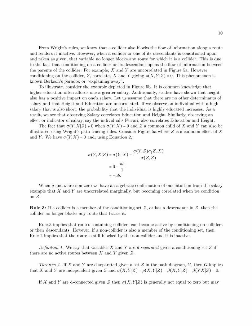
Figure 5: Examples illustrating conditioning on a collider

diagram6. Not only will this technique allow us to derive testable implications of the model forassessing goodness of fit, but it will also be utilized extensively in the analysis of identificationthat follows.

Wright’s rules show that certain routes induce association between variables, while others donot. (We will call routes that induce association in this manner active.) Conditioning on othervariables can change the nature of these routes. Active routes may become inactive, whileinactive routes may become active. In this section, we describe three rules that govern whether agiven route is active or inactive, given a set of conditioning variables. These three rules will beused to determine whether the model implies that variables are conditionally independent given aconditioning set or d-separated. The first rule follows from Wright’s rules.

Rule 1: When no variables are conditioned upon, a route between two variables is active if andonly if it does not contain a collider.

The dependency and information transmitted along an active, non-collider route can beblocked and the route rendered inactive by conditioning on variables along the route. Forexample, consider the path diagram shown in Figure 4, which models the correlation between icecream sales and drownings. When the weather gets warm, people tend to both buy ice cream andplay in the water, resulting in both increased ice cream sales and drowning deaths. In thelanguage of graphical models, ice cream sales and drowning are correlated due to the active route,Ice Cream Sales ← Temperature → Water Activities → Drownings.

However, if we only consider days with the same temperature and/or the same number ofpeople engaging in water activities, then the correlation between Ice Cream Sales and Drowningswill vanish. Thus, conditioning on either Temperature or Ice Cream Sales blocks the flow ofcorrelation transmitted through the route. In general, conditioning on non-colliders along a routeblocks and renders it inactive.

Rule 2: An active route between two variables, X and Y , is rendered inactive by conditioning ona non-collider along that route.

6See also Hayduk et al. (2003), (Mulaik, 2009, ch. 4), and (Kline, 2016, ch. 8) for an introduction to d-separationtailored to SEM practitioners.

10

From Wright’s rules, we know that a collider also blocks the flow of information along a routeand renders it inactive. However, when a collider or one of its descendants is conditioned uponand taken as given, that variable no longer blocks any route for which it is a collider. This is dueto the fact that conditioning on a collider or its descendant opens the flow of information betweenthe parents of the collider. For example, X and Y are uncorrelated in Figure 5a. However,conditioning on the collider, Z, correlates X and Y giving ρ(X,Y ∣Z) ≠ 0. This phenomenon isknown Berkson’s paradox or “explaining away”.

To illustrate, consider the example depicted in Figure 5b. It is common knowledge thathigher education often affords one a greater salary. Additionally, studies have shown that heightalso has a positive impact on one’s salary. Let us assume that there are no other determinants ofsalary and that Height and Education are uncorrelated. If we observe an individual with a highsalary that is also short, the probability that the individual is highly educated increases. As aresult, we see that observing Salary correlates Education and Height. Similarly, observing aneffect or indicator of salary, say the individual’s Ferrari, also correlates Education and Height.

The fact that σ(Y,X ∣Z) ≠ 0 when σ(Y,X) = 0 and Z a common child of X and Y can also beillustrated using Wright’s path tracing rules. Consider Figure 5a where Z is a common effect of Xand Y . We have σ(Y,X) = 0 and, using Equation 2,

σ(Y,X ∣Z) = σ(Y,X) −σ(Y,Z)σ(Z,X)

σ(Z,Z)

= 0 − ab1

= −ab.

When a and b are non-zero we have an algebraic confirmation of our intuition from the salaryexample that X and Y are uncorrelated marginally, but becoming correlated when we conditionon Z.

Rule 3: If a collider is a member of the conditioning set Z, or has a descendant in Z, then thecollider no longer blocks any route that traces it.

Rule 3 implies that routes containing colliders can become active by conditioning on collidersor their descendants. However, if a non-collider is also a member of the conditioning set, thenRule 2 implies that the route is still blocked by the non-collider and it is inactive.

Definition 1. We say that variables X and Y are d-separated given a conditioning set Z ifthere are no active routes between X and Y given Z.

Theorem 1. If X and Y are d-separated given a set Z in the path diagram, G, then G impliesthat X and Y are independent given Z and σ(X,Y ∣Z) = ρ(X,Y ∣Z) = β(X,Y ∣Z) = β(Y X ∣Z) = 0.

If X and Y are d-connected given Z then σ(X,Y ∣Z) is generally not equal to zero but may

11

equal zero for particular parameter values. For example, it is possible that the values of thecoefficients are such that the active routes between X and Y perfectly cancel one another.

We use the diagram depicted in Figure 2 as an example to illustrate the rules of d-separation.In this example, X is d-separated from Y by {W,S}. Similarly X is d-separated from Y by {T}.However, X is not d-separated from Y by {W,S,V } since conditioning on V opens the colliderroute X ⇠⇢ V ← T → Y . Finally, V is not d-separated from W by conditioning on T since T is adescendant of X, opening the collider routes W ⇠⇢X ⇠⇢ V and W →X ⇠⇢ V .

The concept of d-separation formalizes the intuition that routes carry associationalinformation between variables and that this flow of information can be blocked by conditioning.This intuition drives many of the results in identification and assessing goodness of fit that will bediscussed in subsequent sections, making it an essential component of graphical modeling.

We conclude this section by noting that d-separation can be used to derive vanishing partialcorrelations in both recursive and non-recursive models (Spirtes, 1995). Further, all vanishingpartial correlations implied by a path model can be obtained using d-separation (Pearl, 2009, ch.1.2.3). Finally, in fully recursive models where the variables are Gaussian, these vanishing partialcorrelations represent all of the model’s testable implications, a point elaborated later.

3. Identification

Earlier, we discussed how a parameter is identified if the model implies that it is equal tosome function of the implied probability distribution (e.g. covariance matrix). When identified,estimating the necessary aspects of the distribution (typically the sample covariance matrix inlinear models) yields an estimate of the identified parameter. In contrast, if the model does notrestrict the parameter to a single value in terms of the distribution, then it is not identified. Inother words, the parameter is not identified if the model implies that it can be equal to multiple(often infinite) values in terms of the distribution. Clearly, any non-identified parameter cannotbe estimated from data. When all of the model parameters are identified, then we say the modelis identified. If a single parameter is not identified, we say the model is not identified.

In practice, a model’s parameters are often estimated by submitting the data and modelspecification to a computer program, which attempts to find the parameter values that best fitthe data. When the model is identified, then the fitting procedures used by typical software are aconvenient way to estimate the model parameters. Additionally, some of these methods, e.g. fullinformation maximum likelihood (FIML), have been shown to be at least as asymptoticallyefficient as any other consistent estimator. In other words, as the sample size goes to infinity, theFIML estimator has smaller than or equal variance to any other estimator.

However, if the model is not identified, then the program will typically be unable to fit themodel and the procedure will exit with failure7. If they are unable to get the fitting procedures toconverge without issue, researchers typically conclude that the model is not identifiable. Whileconvenient, there are a number of disadvantages to determining identifiability of and estimating

7In other cases, a solution is generated, but it is inadmissible. When this happens, the program generally issuesa warning (e.g. there is a Heywood case). In some cases, however, there is neither a warning in the output nor aHeywood case in the solution.

12

Figure 6: Path model where UY is independent of X given W1, ...,Wk

model parameters in this way. First, if the procedure fails, it is not clear whether it failed due toidentification or other issues (Kenny and Milan, 2012). Second, in rare cases, the procedure willprovide solutions, even when the model is not identified. In such cases, the solutions will beincorrect, and the modeler may have no indiciation that this is the case. Third, when the model isnot identified, the program is not helpful in indicating which parameters are not identifiable(Kenny and Milan, 2012). Fourth, since these methods attempt to simultaneously fit all of themodel’s parameters, misspecification may allow errors to propagate and bias parameter estimatesthroughout the model, rather than isolating the effects of misspecification locally (Bollen et al.,2007). Lastly, if the model is not identifiable, the researcher is only given indication of this factafter she has spent the effort and time to collect data (Kenny and Milan, 2012).

In this section, we introduce two basic graphical criteria for determining whether a givenparameter is identified. When satisfied, these criteria also provide an expression for the parameterin terms of the covariance matrix, allowing the researcher to obtain an estimate for the parameterfrom the sample covariance matrix. As a result, even if the model is not identifiable, the researchercan still obtain estimates of parameters that are identifiable, and she knows which parameters areresponsible for non-identifiability. Additionally, the estimates that are obtained using thesemethods are less likely to be biased by misspecification in unrelated parts of the model (Bollenet al., 2007). Lastly, graphical criteria for identification do not require data, so the researcher candetermine the identifiability of the model or key parameters prior to collecting data.

3.1. Selecting Regressors

Consider the structural equation,

Y = αX + γ1W2 + ... + γkWk +UY

and its corresponding path diagram shown in Figure 6. Because X is uncorrelated with UY givenW = {W1, ...,Wk}, we know that α is identified and equal to the coefficient of X in the regressionof Y on X,W1, ...,Wk. In other words, we can identify and estimate α by “controlling” or“adjusting” for the confounders, W1, ...,Wk. This fact can also be seen from a graphical modelingperspective. By conditioning on W , we block all routes between X and Y except the path from Xto Y . As a result, the partial correlation between X and Y given W is due only to the pathX → Y , and the regression coefficient, β(Y,X ∣W ) is equal to the path coefficient α.

13

It turns out that any set of variables, not just variables in the structural equation for Y , canpotentially be used for control or adjustment in this manner. In general, if there exists a set ofvariables W that blocks all routes between X and Y other than the path X → Y and does notcontain a descendant of Y , then α = β(Y,X ∣W ) and can be estimated using ordinary least squares(OLS). This criterion, called single-door, characterizes when a path coefficient can be estimatedusing OLS8.

Theorem 2. (Pearl, 2009, ch. 5.3.1) (Single-door Criterion) Let G be any acyclic causal graphin which α is the coefficient associated with the path X → Y , and let Gα denote the diagram thatresults when X → Y is deleted from G. The coefficient α is identifiable if there exists a set ofvariables W such that (i) W contains no descendant of Y and (ii) W d-separates X from Y inGα. If W satisfies these two conditions, then α is equal to the regression coefficient β(Y,X ∣W )9,and we say that W is a single-door admissible. Conversely, if W does not satisfy these conditions,then β(Y,X ∣W ) is not equal to α (except in rare instances where spurious routes cancel).

In Figure 3a, we see that W blocks the back-door route X ← Z →W → Y and X isd-separated from Y by W in Figure 3b. Therefore, α is identified and equal to β(Y,X ∣W ). Thisis to be expected since X is independent of UY given W in the structural equation,Y = αX + cW +UY . (This independence can, of course, be verified by explicitly adding UY to thepath diagram and applying d-separation, as in Figures 7a and 7b.) Theorem 2 tells us, however,that Z can also be used for adjustment since Z also d-separates X from Y in Figure 3b, and weobtain α = β(Y,X ∣Z)10. Consider, however, Figure 3c. Variable Z satisfies the single-doorcriterion but W does not. Being a collider, W opens the route, X ← Z →W ↔ Y , in violation ofTheorem 2, leading to bias when adjusting for W . In conclusion, α is equal to β(Y,X ∣Z) inFigures 3a and 3c. However, α is equal to β(Y,X ∣W ) in Figure 3a only.

The intuition for the requirement that Z not be a descendant of Y is depicted in Figures 7aand 7b. We typically do not display the error terms, which can be understood as latent causes. InFigure 7b, we show the error terms explicitly. It should now be clear that Y is a collider andconditioning on Z will create spurious correlation between X, UY , and Y leading to bias ifadjusted for. This means that α can be estimated by the regression slope of Y on X, but addingZ to the regression equation would distort this slope, and yield a biased result.

8A variation of the single-door criterion, called the back-door criterion, graphically characterizes when a totaleffect can be identified and estimated using OLS (Pearl, 2009; Chen and Pearl, 2014). This criterion can be easilyverified by inspecting the diagram and regarded as both a simplification and a generalization of the Alwin and Hauser(1975) method for the case where some errors are correlated.

9The estimand β(Y,X ∣W ) applies whether the variables are standardized or not.

10It turns out, however, that the choice of W is superior to that of Z in terms of estimation power (Kuroki andMiyakawa, 2003). The intuition here is that W is closer in the causal diagram (i.e. a more proximal cause) to Y ,and, therefore, more effective at reducing variations in Y due to uncontrolled factors.

14

(a)

(b)

Figure 7: Example showing that adjusting for a descendant of Y induces bias in the estimation ofα

(a) (b)

Figure 8: (a) Z qualifies as an instrumental variable (b) Z is an instrumental variable given W

3.2. Instrumental Variables

In Figure 8a, no single-door admissible set exists for α and it cannot be estimated using OLS.However, assuming without loss of generality that the variables are standardized and using

Wright’s equations, we see that σ(Y,Z) = γα and σ(X,Z) = γ. As a result, α = σ(Y,Z)σ(X,Z) . In this

case, we were able to identify α using Z as an instrumental variable (IV). Typically, when α isidentified using an IV, it is estimated using two-stage least squares (2SLS) regression.

In this example, we were able to identify α because the covariance between Z and Y could befactored into σ(X,Z) and α, i.e. σ(Y,Z) = σ(Y,X)α. Using Wright’s rules, it is easy to see thatthis will be the case whenever each active route between Z and Y includes the path X → Y .Thus, we can graphically characterize an IV for α, the coefficent from X to Y , as any variable Zthat is d-separated from Y when we remove the path for α, X → Y , from the diagram.

A natural question to ask is whether active routes between Z and Y that do not includeX → Y can be blocked by conditioning. The answer is yes, so long as the conditioning set W doesnot contain any descendants of Y . The following is a graphical definition for instrumentalvariables that can be used to determine whether a given variable is an IV for a coefficient,conditional on W .

Definition 2. (Brito and Pearl, 2002) A variable Z is a instrumental variable given a set Wfor coefficient α (from X to Y ) in a diagram G if

(i) W contains only non-descendants of Y

15

(ii) W d-separates Z from Y in the subdiagram Gα obtained by removing path X → Y from G

(iii) W does not d-separate Z from X in Gα

To demonstrate the usage of Definition 2, consider the following adapation of an example byImbens (2014). Suppose that our goal is to estimate the effect α of a training program X onearnings Y . Since employees are not randomly assigned to the training program, there are anumber of possible unobservable confounding factors that prevent us from directly estimating thecausal effect. Employees that choose to participate may be more ambitious than employees thatdo not. Alternatively, employees that choose to participate may do so because they are sufferingfrom poor performance.

Proximity to the training program Z is a possible instrumental variable since employees thatlive close to the training program are more likely to attend it. In this example, we will evaluatewhether Z is indeed an instrument for α in four possible scenarios.

(i) The training program is located in the workplace. In this case, proximity Z may affect thenumbers of hours employees spend at the office W since they spend less time commuting,and this, in turn, may affect their earnings Y .

(ii) Not only is the training program located in the workplace, but the efficiency of the workers(unmeasured) affects both the number of hours W and their salary Y .

(iii) While proximity may affect the number hours spent in the office, the number of hours spentat the office W does not affect earnings Y because workers in this industry can easily workfrom home. However, efficiency continues to affect both number of hours in the office W andsalary Y .

(iv) Number of hours W again does not affect earning Y . However, work efficiency not onlyaffects salary, but also whether they attend the program because less efficient workers aremore likely to benefit from training.

Figures 9a-9d are the path diagrams for scenarios (i)-(iv) respectively. In each of thesediagrams W is not a descendant of Y , and W does not separate Z from X in Gα. As a result, weonly need to evaluate condition (ii) of Definition 2. In Figure 9a, we see that Z is a conditionalinstrument for α given W because Z is d-separated from Y given W in Gα. However, in Figure9b, α cannot be identified using instruments. Attempting to block the spurious path Z →W → Yactivates another spurious path Z ↔W ↔ Y . In Figure 9c, Z is an instrument for α as long as wedo not condition on W since W is a collider on the path Z ↔W ↔ Y . Similarly, in Figure 9d, Zis an instrument for α if we do not condition on W .

In the SEM literature, instrumental variables are typically defined relative to an equationrather than to a specific path or parameter as we have. By defining an instrument relative to aparameter, researchers can use instruments to identify and estimate individual parameters, evenwhen the equation as a whole is not identified. Also, defining instruments relative to parameters,rather than equations, refines the conditions for when the equation, as a whole, is identifiable.Bollen (2012) notes that a necessary condition for an equation to be identified using instrumental

16

(a) (b) (c) (d)

Figure 9: (a) Z is an conditional instrument for α given W (b) α is not identifiable using instruments(c) Z is an instrument for α (d) Z is an instrument for α

variables is that there are at least as many instruments as there are path coefficients in thestructural equation; however, this condition is not sufficient. Instead, a sufficient condition is thateach path coefficient in the equation has an instrumental variable. Further, a necessary andsufficient condition for the equation to be identified using IVs is that each path coefficient has anindependent instrument. See Brito and Pearl (2002) definition for a precise, graph-baseddefinition of independent instruments.

Lastly, we note that the single-door criterion and the graphical definition of instrumentalvariables can also be applied to SEMs with latent variables like CFA models. See Chen and Pearl(2014) for details.

3.3. Related Work

In theory, the identifiability of any linear-normal path model can be determined by analyzingthe equations that characterize the implied covariance matrix in terms of the model parameters.If the model is partially recursive, these equations can be obtained using Wright’s rules. If themodel contains cycles, then they can also be obtained using matrix algebra (Bollen, 1989). Oncethese equations are obtained, determining whether any particular parameter can be solved for canbe done using Grobner basis methods, mathematical techniques for solving systems of polynomialequations. However, these methods are incredibly slow (a four-variable model can take over threedays to solve using standard computers), and no efficient algorithm for solving this system ofequations exists. Finding efficient algorithms for determining identifiability of linear-normalmodels is an area of ongoing research. Currently, there are a number of sufficient methods foridentifying path models and their coefficients. However, none of them are complete. In otherwords, if they are unable to identify a particular coefficient, it may still be the case that thecoefficient is identifiable, but the algorithm was not able to do so. In this subsection, we survey anumber of recent graphical methods for identification, whose details are beyond the scope of thispaper. Instead, we refer the reader to the relevant literature for more information.

In the section on Instrumental Variables, we mentioned that Brito and Pearl (2002)characterize when an equation can be identified using multiple instruments. Brito and Pearl(2006) generalized this instrumental set method to systematically identify all of the coefficients ina partially recursive model. A similar, but more powerful method was proposed by Foygel et al.

17

(2012) to determine identifiability of a larger set of models11. Additionally their criterion, calledhalf-trek, applies to both partially recursive and non-recursive diagrams. The half-trek algorithmwas further generalized by Chen et al. (2014), Drton and Weihs (2016), and Chen (2016). Lastly,Chen et al. (2016) and Chen et al. (2017) provided a method for generating new instrumentalvariables when some of the models parameters are known or identified. They used this method toprovide an identification algorithm that is able to identify strictly more coefficients and modelsthan the half-trek methods.

Other graphical methods for identification in linear path models include Tian (2005), Tian(2007), and Tian (2009). These methods identify parameters by converting the structuralequations into orthogonal partial regression equations. Tian (2005) also gave a method fordecomposing a complex path diagram into simpler sub-diagrams, showing that the originaldiagram is identifiable if and only if the sub-diagrams are.

Do-calculus (Pearl, 2009) and non-parametric algorithms for identifying causal effects (Tianand Pearl, 2002; Tian, 2002; Shpitser and Pearl, 2006; Huang and Valtorta, 2006), which havebeen proven to be complete for identifying causal effects in non-parametric models, may also beapplied to parameter identification in path models (Chen and Pearl, 2014) (even when these pathmodels do not represent causal relations).

Lastly, Rigdon (1995) described a set of necessary and sufficient graphical rules for theidentification of nonrecursive models where the endogenous variables can be partitioned into setsof recursively-related blocks of size two or one.

4. Deriving Testable Implications

All methods for evaluating goodness of fit compare statistical constraints that are implied bythe model specification with an assessment of the degree to which those constraints are satisfiedin the data. The most common methods use computer software to first estimate the values of themodel parameters from sample data and then, taking those estimates at face value, compute themodel-implied covariance matrix. This model-implied covariance matrix is then compared to thesample covariance matrix using statistical tests, such as the well-known model chi-square test inSEM. The advantage of these methods are that they conveniently and simultaneously test all ofthe restrictions implied by the model on the covariance matrix.

However, there are a number of disadvantages, as well. First, they cannot be used unless themodel is identified. Second, poor overall fit of the model does not provide the modeler withinformation about which aspect of the model needs to be revised12. Finally, it is possible that aglobal and simultaneous test will not reject the model, even when a crucial testable implication isviolated. Global fit statistics, such as the model chi-square, Bentler Comparative Fit Index (CFI),

11Foygel et al. (2012) also released an R package implementing their algorithm called SEMID, which determineswhether the entire model is identifiable given its path diagram.

12 While modification indices can be used, they are restricted by the requirement that each modification resultsin an identified model. Additionally, they assume that, other than the specific path being investigated, the originalmodel is correct. Lastly, they can be misleading if the model fails to fit for a reason other than a missing or wrongpath, such as non-normality (Thoemmes et al., 2018).

18

and Steiger-Lind root mean square error of approximation (RMSEA), among others, measureonly average or overall fit of the model to the sample covariance matrix. Thus, it can and doeshappen that values of global fit statistics mask violations of individual testable implications(Tomarken and Waller, 2003). Moreover, these masked violations may indicate a misspecificationthat is crucial for decision making.

In this section, we describe how individual testable implications of the model can be obtainedfrom the graphical tools given in previous sections. These implications can be tested even whenthe model is not identified, the statistical power of each test is greater than that of a global test(McDonald, 2002; Bollen and Pearl, 2013), and, in the case of failure, the researcher knows exactlywhich implication of the model was violated, obtaining guidance when re-specifying the model.

When the model is identified, the results of these local tests should be reported in addition tothe global fit statistics13. When the model is not identified, researchers can still evaluate its localfitness requirements and utilize the aforementioned methods of identifying and estimatingindividual parameters, which may be of significant research interest.

4.1. Vanishing Correlation Constraints

The method of d-separation allows modelers to derive conditional independence constraintsimplied by the path model simply by inspecting the diagram. In the case of recursive modelswithout equality constraints, the number of implied conditional independences exactly equals themodel degrees of freedom, or dfM . For example, if dfM = 5 for a recursive model, then there are atotal of five partial correlations that should vanish (equal zero), given the configuration of pathsspecified in the model. These five vanishing partial correlations represent all the constraints thatthe model specification imposes on the covariance matrix. As a result, they represent all thetestable implications of the model, assuming that the endogenous variables are normallydistributed (Geiger and Pearl, 1993). The model chi-square test, where dfM = 5 for the samegraph, can be seen as an overall significance test of whether all five partial correlations vanish,but inspecting the values of the individual sample partial correlations provides all the detailsbehind the global chi-square test. Additionally, since these conditional independence constraintsare derived, using d-separation, from specific aspects of the model specification, the modelerknows which aspects of the model are incorrect when one of these constraints is violated. It is inthis sense that we say such tests assess “local” rather than “global” fit.

For example, in Figure 10a, we obtain the following vanishing partial correlations:ρ(V2,V3∣V1) = 0, ρ(V1,V4∣V2,V3) = 0, ρ(V2,V5∣V4) = 0, and ρ(V3,V5∣V4) = 0. Hypothesis testingwhether these partial correlations are equal to zero from data can be accomplished using theFisher Z transformation, which is implemented in many standard statistical computer tools andthe DAGitty R package (Textor et al., 2011; Thoemmes et al., 2018). If a test shows that aconstraint, say ρV2V3.V1 = 0 does not hold in the data, we have reason to believe that the modelspecification is incorrect and should reconsider the lack of a path between V2 and V3.

In some cases, vanishing partial correlations derived from d-separation may be redundant. In

13A serious flaw in many, if not most, published SEM studies is the failure to report information about local fit(Vermeulen and Hartmann, 2015; Goodboy and Kline, 2017).

19

(a) (b)

Figure 10: (a) Example illustrating vanishing partial correlation (b) The skeleton of the model in(a)

other words, some may be implied by others. There are ways to derive minimal sets of impliedvanishing partial correlations, called basis sets, that consist of the smallest number of conditionalindependences that imply all others for a particular diagram. For the same diagram, there may bemultiple basis sets, each with the same overall number of conditional independences, that can bederived using different but logically-consistent methods to generate a basis set. We do not coverbasis sets here, but see Kang and Tian (2009), Pearl (2009, pp. 142-145), or Shipley (2000, pp.61-63) for more information.

Lastly, d-separation can also be used to derive conditional independence constraints in latentvariable models. See Thoemmes et al. (2018) for details, as well as additional graphical tools forlocal fit evaluation of latent variable models.

4.2. Overidentifying Constraints

In the previous subsection, it was noted that all of the testable implications of a recursiveand normal path model take the form of vanishing partial correlation constraints that can bederived using d-separation. Non-recursive and partially recursive models, however, may implyother types of constraints on the covariance matrix. Some of these constraints can be derived byidentifying parameters using two or more distinct identification strategies14. Such parameters areoften called overidentified.

Consider the path diagram shown in Figure 11. Since W satisfies the single-door criterion forα, the path model implies that α = β(Y,X ∣W ). Additionally, Z is an IV for α so the model also

implies that α = β(Y,Z)β(X,Z) . In this case, we say that α is overidentified, and we obtain a testable

implication of the model by equating the two expressions, β(Y,X ∣W ) andβ(Y,Z)β(X,Z) . If the data does

not corroborate this equality, then the researcher has reason to believe that the model ismisspecified, and it does not fit the data. Specifically, there is evidence that the model restrictions

14See Pearl (2004) for a formal definition of “distinct identification strategies”.

20

Figure 11: α is overidentified using W as a single-door admissible set and Z as an IV

that allow Z to be an IV (e.g. the lack of a path between Z and Y ) are incorrect, or the modelrestrictions that allow {W} to be a single-door admissible set (e.g. the lack of a bidirected pathbetween W and X and the lack of a bidirected path between X and Y ) are, or both.

The single-door criterion and IVs provide researchers with a systematic way to derive theseoveridentifying constraints. (See Chen et al. (2017) for graphical algorithm that discoversoveridentifying constraints using more complex identification methods). Hypothesis testing canthen be conducted using the Durbin-Wu-Hausman test, also called the Hausman specification test(Hausman, 1978). This test is commonly implemented in standard statistical computer tools.

When two single-door admissible sets exist for a coefficient, the corresponding overidentifyingconstraint will always be equivalent to a vanishing partial correlation constraint that could alsohave been derived using d-separation (Chen and Pearl, 2015). In contrast, overidentifyingconstraints derived from two different IVs or a single-door admissible set and an IV, may yieldother types of constraints that cannot be obtained from d-separation.

4.3. Equivalent Models

Since conditional independences represent all of the constraints a recursive path modelimposes on the covariance matrix, two recursive models that share the same implied conditionalindependences cannot be distinguished using the sample covariance matrix. In such cases, we saythat the models are covariance equivalent. If the endogenous variables are normally distributed,then covariance equivalence implies general equivalence and the models cannot be distinguishedfrom data at all. Most authors of SEM studies fail to acknowledge the existence of equivalentmodels, which is a serious form of confirmation bias (Hoyle and Isherwood, 2013).

Researchers can check whether two models share the same implied conditional independencesusing d-separation. However, in complex models with many variables, applying the d-separationcriterion by hand can be tedious. Instead, if the diagram does not contain bidirected paths, modelequivalence can be checked by simply noting whether the two models have the same skeleton andv-structures (Pearl, 2009, pp.145-149). (If the diagrams have bidirected paths, we can still applythis method by first replacing each bidirected path with a latent common cause. For example, thebidirected path X ⇠⇢ Y is replaced with X ← U → Y .) The skeleton is the undirected diagramobtained by replacing all arrows with undirected paths, which are depicted in the diagram using−−. For example, the skeleton for Figure 10a is Figure 10b. V-structures are two convergingarrows whose tails are not connected by an arrow. For example, V2 → V4 ← V3 is the onlyv-structure in Figure 10a.

Theorem 3. (Verma and Pearl, 1990) Two recursive and normal path models are covarianceequivalent if and only if they entail the same sets of zero partial correlations. Moreover, two such

21

(a) (b) (c)

Figure 12: Models (a), (b), and (c) are equivalent.

Figure 13: Counterexample to the standard Replacement Rule; The arrow X → Y cannot bereplaced.

models are covariance equivalent if and only if their corresponding graphs have the same skeletonsand the same sets of v-structures.

The graphs in Figures 12a, 12b, and 12c are equivalent because they share the same skeletonand v-structures. Note that we cannot reverse the path from V4 to V5 since doing so wouldgenerate a new v-structure, V2 → V4 ← V5.

The graphical criterion given in Theorem 3 is necessary and sufficient for equivalencebetween recursive path models with normally-distributed endogenous variables. It is a necessarycondition for equivalence between non-recursive models since d-separation in the diagram impliesvanishing partial correlation in the covariance matrix. In contrast, the more prevalentreplacement criterion (Lee and Hershberger, 1990) is not always valid15. Pearl (2012) gave thefollowing example depicted in Figure 13. According to the replacement criterion, we can replacethe path X → Y with a bidirected path X ↔ Y and obtain a covariance equivalent model when allpredictors (Z) of the effect variable (Y ) are the same as those for the source variable (X).Unfortunately, the post-replacement model imposes the constraint, ρ(WZ ∣Y ) = 0, which is notimposed by the original model. This can be seen from the fact that, conditioned on Y , the routeZ → Y ←X ↔W is unblocked and becomes blocked if replaced by Z → Y ↔X ↔W . The sameapplies to the route Z →X ↔W , since Y would cease to be a descendant of X.

15The replacement rule violates the transitivity of equivalence (Hershberger and Marcoulides, 2006), yet it is stillused in most of the SEM literature (Mulaik, 2009; Williams, 2012, pp. 247-260).

22

5. Computer Tools

There are freely-available computer tools for analyzing directed acyclic graphs thatautomatically apply the graphical methods just described. Directed acyclic graphs (DAGs)corresponds to a recursive or partially recursive path diagram. In other words, they do not allowcycles. While the tools presented in this paper can be additionally applied to cyclic graphs andfully nonrecursive path models, much of the software developed has focused on directed acyclicgraphs.

Some of these computer tools are stand-alone applications for installation on personalcomputers, but others are online applications that analyze graphs drawn by the user in anInternet browser. All such tools support the evaluation of a path diagram in the planning stagesfor a study. Some of these tools are described next. This list is not comprehensive, but all thesetools help researchers to reap the potential benefits of analyzing their graphs and thus testingtheir ideas before collecting the data:

1. The DAGitty program is web-based tool for analyzing causal graphs that can also be usedoffline (Textor et al., 2011). It evaluates whether direct or total effects are identified eitherthrough covariate selection or through the analysis of instruments. It also lists conditionalindependences implied by the graph.

2. Textor et al. (2011) also developed a DAGitty R package that includes the functionality ofthe web-based tool. Thoemmes et al. (2018) extended this package to include tests forvanishing partial correlation and to implement additional graphical methods for analysis oflatent variable models.

3. The Belief and Decision Network Tool (Knoll et al., 2008) is a Java applet for learningabout the concept of d-separation. For example, after drawing a graph onscreen, thisprogram can then be optionally run in ask the applet mode, where the user clicks on twofocal variables and a set of covariates, and the program automatically indicates whether thefocal variables are independent, given those covariates.

4. The dagR package for R (Breitling, 2010) provides a set of functions for drawing,manipulating, and analyzing directed acyclic graphs and also simulating data consistentwith the corresponding diagram. It can evaluate effects of analyzing different subsets ofcovariates when estimating causal effects of exposure variables on outcome variables, amongother capabilities. Graphs are specified in syntax, but the corresponding graph of the modelcan be manipulated in the R environment.

6. Example Problem

In this section, we present an illustrative example to demonstrate how typical analysis can beexpanded and improved by incorporating ideas from graphical modeling, thereby creating anexpanded and improved overall practice. Presented in Figure 14a is a variation on a path modelanalyzed by Roth et al. (1989). We assume a linear model with continuous variables. Thehypotheses are that

23

(a)(b)

Figure 14: (a) Example path model, where E represents exercise, H mental hardiness, F physicalfitness, and S stress (b) The same model as it would be expressed in the DAGitty computer tool,where U1 and U2 are latent variables

1. exercise (E) and mental hardiness (H) covary;

2. variables E and H each indirectly affects health problems (P ) through, respectively,physical fitness (F ) and stress (S); and

3. the errors of F and P covary; that is, they share an unmeasured common cause.

Standard practice dictates that once the model has been specified, the best fit for the modelparameters should be determined using data. If the model is not identifiable, then this procedurewould fail. At this point, researchers would be forced to respecify the model or collect data onadditional variables that may enable identification. The former is clearly not an ideal solutionbecause model specification should be based on reality and not used as a workaround foridentification issues. The latter can be difficult to accomplish since standard SEM programs donot provide the researcher with pointers to the variables that would enable identification. Thus,the researcher may take the time and resources to collect data on new variables, only to find thatthe model is still not identified.

In contrast, graphical tools may enable researchers to estimate coefficients of interest (e.g.the effect of stress, exercise, or mental hardiness on health problems) even when the model, as awhole, is not identified. If these quantities are also not identifiable, then the researcher can stilluse graphical tools to determine which additional variables would enable identification. She wouldsimply add the variable in question to the path diagram and use the tools described above todetermine whether the model or coefficients of interest are now identified.

Next, we describe how the graphical identification methods described in this paper can beused to identify and estimate each of the coefficients in Figure 14a. Readers can verify theidentification results and testable implications for this example using DAGitty. Error correlationsare represented in DAGitty by specifying latent variables as common causes, such as U1 and U2 inFigure 14b. See the appendix for code that automatically generates the graph for this example inDAGitty.

The total number of available identification stategies reported by DAGitty is indicated inparentheses for each coefficient listed next:

1. F → P (3). The DAGitty tool indicates that the coefficient for this direct effect is identifiedthrough the instruments E given S and H given S. Controlling for S in each instrument

24

EstimatorCoefficient OLS 2SLS

E → F .108 (∅) -.646 (H).719 (S)

H → S -.203 (∅) 1.469 (E)-1.637 (F )

F → P — -.558 (E∣S)-6.927 (H ∣S)-.734 (E∣H)

S → P .628 (E) 1.161 (H ∣F,E).597 (H)

Table 1: Estimators of coefficients for Figure 14

d-separates variables E and H from the outcome P in the modified graph without F → P .Similarly, the direct effect is identified by the instrument E given H.

2. S → P (3). Two different single-door admissible sets, E and H, identify the direct effect:Controlling for either E or H blocks the back-door route S ←H ⇠⇢ E → F → P in themodified graph without S → P . The instrument H given {F,E} also identifies the directeffect.

3. E → F , H → S (3 each). There are no back-door treks between either pair of explanatoryand outcome variables; thus, the coefficient for each direct effect can be estimated inbivariate regression (i.e., ∅, the empty set, is single-door admissible). Two differentinstruments are also available for each direct effect, H and S for E → F and E and F forH → S.

A veritable cornucopia of identification strategies are available for this example by applyingconcepts from graphical modeling. Summary statistics (correlations, standard deviations, andmeans) for the observed variables in Figure 14a measured within a sample of 373 universitystudents were analyzed in SPSS in order to generate results for this example. Syntax files withthe data for this analysis summarized in matrix form and output files for SPSS in both plain textand Adobe PDF format can be downloaded from the supplemental materials page for this article.

The estimate for X → Y using Z as an instrument can be obtained by conducting 2SLSregression or directly from the summary statistics by dividing σ(Y,Z) by σ(X,Z), where σ(Y,Z)is the sample covariance between Y and Z and σ(X,Z) is the sample covariance between X andZ. Similarly,

σ(Y,Z ∣W )σ(X,Z ∣W ) (12)

is the estimate for X → Y using an instrument, Z given W .Reported in the top part of Table 1 are unstandardized estimates of direct effects for this

example with conditioning sets given in parenthesis. Since the model has been shown to beidentified, estimates could also be obtained using ML procedures implemented in standard SEM

25

software. As mentioned above, some of these procedures like FIML have been shown to be atleast as asymptotically efficient as any other estimator and, therefore, may be preferable to theestimates provided in Table 1. However, researchers should verify, to the best of their abilities,that the model specification is correct before using estimates derived from graphical or MLmethods.

Typically, researchers inspect the values of global fit statistics provided by standard SEMtools to assess the model’s fit. Values of selected global fit statistics in ML estimation, obtainedusing LISREL and Mplus, for this example are listed next:

χ2M(4) = 10.529, p = .032

RMSEA = .066,90% CI [.017, .116]CFI = .958; SRMR = .051

The model chi-square is marginally significant at the .05 level, and the upper bound of theconfidence interval based on the RMSEA is unfavorable, but other results do not indicate grosslypoor global fit. Through selective reporting (e.g., omit the CI based on the RMSEA) and ignoringthe failed chi-square test–both common practices in the SEM literature (Ropovik, 2015)–aresearcher could potentially argue for retaining the model.

Even if none of the statistics indicate poor fit, it is still important that researchers test themodel using the graphical methods described in this paper. Global fit statistics may fail to detectmisspecification that can greatly bias estimates of important coefficients because they are overallsummaries of the model’s fit (Tomarken and Waller, 2003). In contrast, graphical methods allowresearchers to derive the testable implications that underlie global fit statistics and test themindividually.

If the researcher does find the global fit statistics to be problematic, d-separation and theabove identification criteria also enable the researcher to determine exactly which testableimplications are violated and revise the model accordingly. In contrast, the modification indicesprovided by standard SEM software are restricted by the requirement that each modificationresults in an identified model. Additionally, they assume that, other than the specific path beinginvestigated, the original model is correct. Lastly, they can be misleading if the model fails to fitfor a reason other than a missing or wrong path, such as non-normality (Thoemmes et al., 2018).Next, we demonstrate how to use graphical tools to test and revise the model shown in Figure 14a.

Inspecting Table 1 immediately reveals issues with the model fit. Estimates for E → F andH → S vary appreciably in both direction and magnitude, and thus are inconsistent. This patternattests to likely specification error. For example, the individual 2SLS estimates for E → F , −.646and .719 (see the table), each assumes that the corresponding instrument, respectively, H and S,has no direct effect on F . Additionally, they assume that there is no bidirectional route thatconnects either instrument just mentioned with F (see Figure 14a). At least one of theseassumptions is wrong and the researcher can use this information to revise the model accordingly.

Estimates of F → P agree in direction (all negative) but appreciably vary in magnitude; therange is -6.927 to -.558 (see Table 1). The outlier value, or -6.927, is from the 2SLS analysis thatassumes no direct effect between variables H and P . Values of multiple estimates for S → P areall > 0 and generally similar in magnitude (.597 to 1.161), which is more reassuring.

26

Conditional Independence Partial Correlation p

E ⊥ S∣H -0.058 0.264H ⊥ F ∣E 0.089 0.086F ⊥ S∣H -0.117 0.024F ⊥ S∣E -0.120 0.020

H ⊥ P ∣E,S -0.093 0.074

Table 2: Implied conditional independences for Figure 14

Figure 15: Flow chart depicting expanded practice that combines techniques from graphical mod-eling and standard path analysis. Steps utilizing graphical modeling and standard path analytictechniques indicated by (GM) and (PA) respectively.

Applying d-separation also reveals implications that can be use to test the model. Listednext are five vanishing partial correlations implied by Figure 14a:

ρ(E,S∣H) = ρ(H,F ∣E) = ρ(F,S∣E) = ρ(F,S∣H) = ρ(H,P ∣ES) = 0

Table 2 shows the sample partial correlations and their p-value for the hypothesis that thepopulation partial correlations are equal to zero. The tests for ρ(F,S∣E) = 0 and ρ(F,S∣H) = 0fail at the 5% significance level, suggesting that F and S should not be d-separated by either Enor H. The simplest revision to the model specification would include an edge between F and S.The lack of this edge in Figure 14a could also explain the inconsistent 2SLS estimates for E → F ,H → S, and F → P shown in Table 1.

Once the model has been revised, the researcher should repeat the procedure described above

27

until she obtains a model that passes both global and local tests for goodness of fit. At this point,it is important to consider equivalent models, which can be derived using the graphicalprocedures described above. If she still feels confident that the model specification is correct, thenestimated values for the model parameters can be obtained using either standard SEM softwareor OLS/2SLS. The former may be preferable when the model specification is correct due to betterefficiency. The latter may be preferable when the researcher is unsure about the modelspecification due to equivalent models or borderline results for fit tests, since they may isolateerrors rather than allowing them to propagate (Bollen et al., 2007). This procedure is summarizedin a flow chart depicted in Figure 15.

7. Conclusion

The benefits of causal graphs are usually attributed to their ability to represent theoreticalassumptions visibly and transparently, by abstracting away unnecessary algebraic details. Not aswidely recognized among practitioners of SEM is the inferential power of analyzing graphs apartfrom analyzing the data. We demonstrated how a few basic graphical tools can be applied to awide variety of modeling tasks in experimental psychology. Specifically, we showed how thesetools can determine the identification status of path coefficients through both partial regressionand IV methods. We further demonstrated how to derive testable implications throughoveridentification and the reading of vanishing partial correlations, both giving rise to newmethods for assessing local fit. Finally, we discussed the identification of equivalent models, andillustrated the application of these tools and methods through numerical examles.

Appendices

A. DAGitty Model Code for Figure 14a

Copy the text below and paste it in the model code window of DAGitty in order for the pathdiagram to be to automatically drawn. The blank line must be retained in order for the code tocorrectly execute.

E 1 @−1.300 , −0.500F 1 @−0.700 , −0.500H 1 @−1 .300 ,0 .300P 1 @−0.200 , −0.100S 1 @−0 .700 ,0 .300U1 U @−1.800 , −0.100U2 U @−0.250 , −0.450

E FF PH SS P

28

U1 E HU2 F P

References

Alwin, D. and Hauser, R. (1975). The decomposition of effects in path analysis. AmericanSociological Review 40 37–47.

Blalock, H. (1962). Four-variable causal models and partial correlations. American Journal ofSociology 68 182–194.

Bollen, K. (1989). Structural Equations with Latent Variables. John Wiley, New York.

Bollen, K. and Pearl, J. (2013). Eight myths about causality and structural equation models.In Handbook of Causal Analysis for Social Research (S. Morgan, ed.). Springer, 301–328.

Bollen, K. A. (2012). Instrumental variables in sociology and the social sciences. AnnualReview of Sociology 38 37–72.

Bollen, K. A., Kirby, J. B., Curran, P. J., Paxton, P. M. and Chen, F. (2007). Latentvariable models under misspecification: two-stage least squares (2sls) and maximum likelihood(ml) estimators. Sociological Methods & Research 36 48–86.

Breitling, L. P. (2010). dagr: a suite of r functions for directed acyclic graphs. Epidemiology21 586–587.

Brito, C. and Pearl, J. (2002). Generalized instrumental variables. In Uncertainty in ArtificialIntelligence, Proceedings of the Eighteenth Conference (A. Darwiche and N. Friedman, eds.).Morgan Kaufmann, San Francisco, 85–93.

Brito, C. and Pearl, J. (2006). Graphical condition for identification in recursive SEM. InProceedings of the Twenty-Third Conference on Uncertainty in Artificial Intelligence. AUAIPress, Corvallis, OR, 47–54.

Chen, B. (2016). Identification and overidentification of linear structural equation models. InAdvances in Neural Information Processing Systems.

Chen, B., Bareinboim, E. and J., P. (2016). Incorporating knowledge into structural equationmodels using auxiliary variables. In Proceedings of the Twenty-fifth International JointConference on Artificial Intelligence (S. Kambhampati, ed.). AAAI Press, Palo Alto, CA,3577–3583.

Chen, B., Kumor, D. and Bareinboim, E. (2017). Identification and model testing in linearstructural equation models using auxiliary variables. In Proceedings of the 34th InternationalConference on Machine Learning (D. Precup and Y. W. Teh, eds.), vol. 70 of Proceedings ofMachine Learning Research. PMLR, International Convention Centre, Sydney, Australia.URL http://proceedings.mlr.press/v70/chen17f.html

29

Chen, B. and Pearl, J. (2014). Graphical tools for linear structural equation modeling. Tech.Rep. R-432, <http://ftp.cs.ucla.edu/pub/stat ser/r432.pdf>, Department of Computer Science,University of California, Los Angeles, CA.

Chen, B. and Pearl, J. (2015). Exogeneity and robustness. Tech. Rep. R-449,<http://ftp.cs.ucla.edu/pub/stat ser/r449.pdf>, Department of Computer Science, University ofCalifornia, Los Angeles, CA. Submitted.

Chen, B., Tian, J. and Pearl, J. (2014). Testable implications of linear structual equationmodels. In Proceedings of the Twenty-eighth AAAI Conference on Artificial Intelligence (C. E.Brodley and P. Stone, eds.). AAAI Press, Palo, CA.<http://ftp.cs.ucla.edu/pub/stat ser/r428-reprint.pdf>.

Cramer, H. (1946). Mathematical Methods of Statistics. Princeton University Press, Princeton,NJ.

Drton, M. and Weihs, L. (2016). Generic identifiability of linear structural equation models byancestor decomposition. Scandinavian Journal of Statistics 43 1035–1045.

Elwert, F. (2013). Graphical causal models. In Handbook of causal analysis for social research.Springer, 245–273.

Foygel, R., Draisma, J. and Drton, M. (2012). Half-trek criterion for generic identifiabilityof linear structural equation models. The Annals of Statistics 40 1682–1713.

Geiger, D. and Pearl, J. (1993). Logical and algorithmic properties of conditionalindependence and graphical models. The Annals of Statistics 2001–2021.

Goodboy, A. K. and Kline, R. B. (2017). Statistical and practical concerns with publishedcommunication research featuring structural equation modeling. Communication ResearchReports 34 68–77.

Hausman, J. A. (1978). Specification tests in econometrics. Econometrica: Journal of theEconometric Society 1251–1271.

Hayduk, L., Cummings, G., Stratkotter, R., Nimmo, M., Grygoryev, K., Dosman, D.,Gillespie, M., Pazderka-Robinson, H. and Boadu, K. (2003). Pearl’s d-separation: Onemore step into causal thinking. Structural Equation Modeling 10 289–311.

Hershberger, S. L. and Marcoulides, G. A. (2006). The problem of equivalent structuralmodels. In Structural equation modeling: A second course (G. R. Hancock and R. O. Mueller,eds.). Information Age Publishing, Greenwich, CT, 3–37.

Hoyle, R. H. (2012). Handbook of structural equation modeling. Guilford Press.

Hoyle, R. H. and Isherwood, J. C. (2013). Reporting results from structural equationmodeling analyses in archives of scientific psychology. Archives of scientific psychology 1 14.

30

Huang, Y. and Valtorta, M. (2006). Pearl’s calculus of intervention is complete. InProceedings of the Twenty-Second Conference on Uncertainty in Artificial Intelligence(R. Dechter and T. Richardson, eds.). AUAI Press, Corvallis, OR, 217–224.

Imbens, G. (2014). Instrumental variables: An econometrician’s perspective. Tech. rep., NationalBureau of Economic Research.

Kang, C. and Tian, J. (2009). Markov properties for linear causal models with correlatederrors. The Journal of Machine Learning Research 10 41–70.

Kenny, D. A. and Milan, S. (2012). Identification: A non-technical discussion of a technicalissue. In Handbook of Structural Equation Modeling (G. M. S. W. R. Hoyle, D. Kaplan, ed.).Guilford Press, New York, 145–163.

Kline, R. (2016). Principles and Practice of Structural Equation Modeling. 4th ed. Methodologyin the social sciences.URL http://books.google.com/books?id=-MDPILyu3DAC

Knoll, B., Kisynski, J., Carenini, G., Conati, C., Mackworth, A. and Poole, D.(2008). Aispace: Interactive tools for learning artificial intelligence. In Proc. AAAI 2008 AIEducation Workshop.

Koller, D. and Friedman, N. (2009). Probabilistic graphical models: principles and techniques.MIT press.

Kuroki, M. and Miyakawa, M. (2003). Covariate selection for estimating the causal effect ofcontrol plans by using causal diagrams. Journal of the Japanese Royal Statistical Society,Series B 65 209–222.

Lee, S. and Hershberger, S. (1990). A simple rule for generating equivalent models incovariance structure modeling. Multivariate Behavioral Research 25 313–334.

McDonald, R. (2002). What can we learn from the path equations?: Identifiability constraints,equivalence. Psychometrika 67 225–249.

Morgan, S. and Winship, C. (2007). Counterfactuals and Causal Inference: Methods andPrinciples for Social Research (Analytical Methods for Social Research). Cambridge UniversityPress, New York, NY.

Mulaik, S. A. (2009). Linear causal modeling with structural equations. CRC Press.

Pearl, J. (1995). Causal diagrams for empirical research. Biometrika 82 669–710.

Pearl, J. (1998). Graphs, causality, and structural equation models. Sociological Methods andResearch 27 226–284.

Pearl, J. (2004). Robustness of causal claims. In Proceedings of the 20th conference onUncertainty in artificial intelligence. AUAI Press.

31

Pearl, J. (2009). Causality: Models, Reasoning, and Inference. 2nd ed. Cambridge UniversityPress, New York.

Pearl, J. (2012). The causal foundations of structural equation modeling. In Handbook ofStructural Equation Modeling (R. Hoyle, ed.). Guilford Press, New York, 68–91.

Pearl, J. (2014). The deductive approach to causal inference. Journal of Causal Inference 2115–129.

Rigdon, E. E. (1995). A necessary and sufficient identification rule for structural modelsestimated in practice. Multivariate Behavioral Research 30 359–383.

Ropovik, I. (2015). A cautionary note on testing latent variable models. Frontiers in psychology6.

Roth, D. L., Wiebe, D. J., Fillingim, R. B. and Shay, K. A. (1989). Life events, fitness,hardiness, and health: A simultaneous analysis of proposed stress-resistance effects. Journal ofPersonality and Social Psychology 57 136.

Shipley, B. (2000). A new inferential test for path models based on directed acyclic graphs.Structural Equation Modeling 7 206–218.

Shpitser, I. and Pearl, J. (2006). Identification of conditional interventional distributions. InProceedings of the Twenty-Second Conference on Uncertainty in Artificial Intelligence(R. Dechter and T. Richardson, eds.). AUAI Press, Corvallis, OR, 437–444.

Spirtes, P. (1995). Directed cyclic graphical representation of feedback. In Proceedings of theEleventh Conference on Uncertainty in Artificial Intelligence (P.Besnard and S. Hanks, eds.).Morgan Kaufmann, San Mateo, CA, 491–498.

Textor, J., Hardt, J. and Knuppel, S. (2011). Dagitty: a graphical tool for analyzing causaldiagrams. Epidemiology 22 745.

Thoemmes, F., Rosseel, Y. and Textor, J. (2018). Local fit evaluation of structural equationmodels using graphical criteria. Psychological methods 23 27.

Tian, J. (2002). Studies in Causal Reasoning and Learning. Ph.D. thesis, Computer ScienceDepartment, University of California, Los Angeles, CA.

Tian, J. (2005). Identifying direct causal effects in linear models. In Proceedings of the NationalConference on Artificial Intelligence, vol. 20. Menlo Park, CA; Cambridge, MA; London; AAAIPress; MIT Press; 1999.

Tian, J. (2007). A criterion for parameter identification in structural equation models. InProceedings of the Twenty-Third Conference Annual Conference on Uncertainty in ArtificialIntelligence (UAI-07). AUAI Press, Corvallis, Oregon.

32

Tian, J. (2009). Parameter identification in a class of linear structural equation models. InProceedings of the Twenty-First International Joint Conference on Artificial Intelligence(IJCAI-09).

Tian, J. and Pearl, J. (2002). A general identification condition for causal effects. InProceedings of the Eighteenth National Conference on Artificial Intelligence. AAAI Press/TheMIT Press, Menlo Park, CA, 567–573.

Tomarken, A. J. and Waller, N. G. (2003). Potential problems with “well fitting” models.Journal of Abnormal Psychology 112 578.

VanderWeele, T. (2015). Explanation in causal inference: methods for mediation andinteraction. Oxford University Press.

Verma, T. and Pearl, J. (1990). Equivalence and synthesis of causal models. In Proceedings ofthe Sixth Conference on Uncertainty in Artificial Intelligence. Cambridge, MA. Also in P.Bonissone, M. Henrion, L.N. Kanal and J.F. Lemmer (Eds.), Uncertainty in ArtificialIntelligence 6, Elsevier Science Publishers, B.V., 255–268, 1991.

Vermeulen, I. and Hartmann, T. (2015). Questionable research and publication practices incommunication science. Communication Method and Measures 9 189–192.

Williams, L. (2012). Equivalent models: Concepts, problems, alternatives. Handbook ofStructural Equation Modeling (R. Hoyle, ed.). Guilford Press, New York 247–260.

Wolfle, L. M. (1980). Strategies of path analysis. American Educational Research Journal 17183–209.

Wright, S. (1921). Correlation and causation. Journal of Agricultural Research 20 557–585.