Graphical)Models - UMass Amherst

Graphical Models

Lecture 16:

Maximum a Posteriori InferenceAndrew McCallum

[email protected]

Thanks to Noah Smith and Carlos Guestrin for some slide materials.1

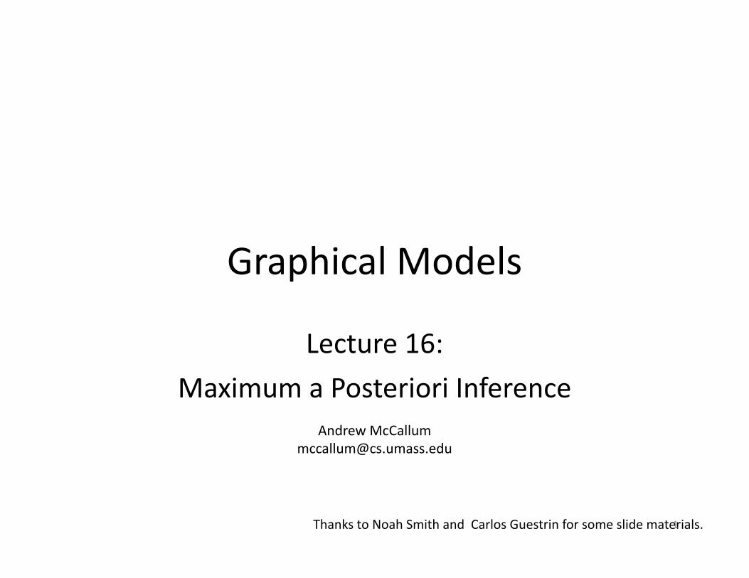
ProbabilisEc Inference

• Assume we are given a graphical model.

• Want:P (X | E = e) =

P (X,E = e)P (E = e)

∝ P (X,E = e)

=�

y∈Val(Y )

P (X,E = e,Y = y)

Lecture 9

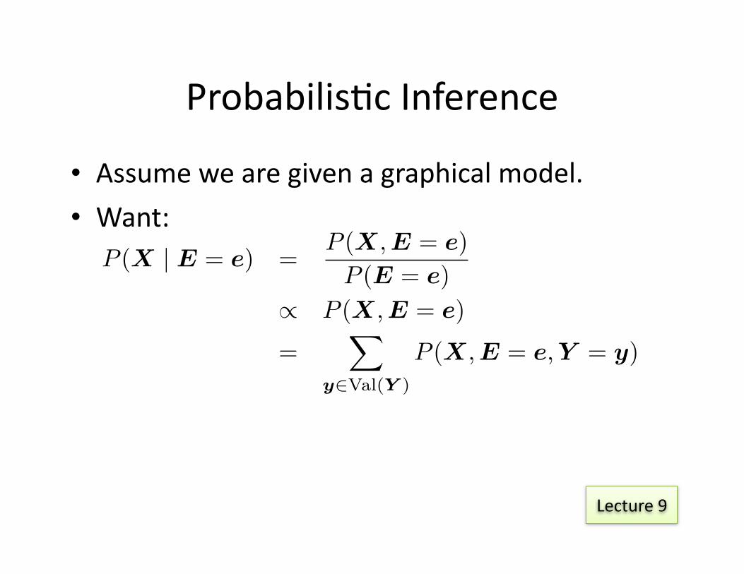
Inference: Where We Have Been

9. Variable eliminaEon10.Variable eliminaEon, conEnued11.Clique trees, sum-‐product message passing,

calibraEon12.Sum-‐product-‐divide (belief update)

message passing13.Mean field variaEonal inference14.Cluster graphs, generalized loopy belief

propagaEon15.Sampling, Monte Carlo Markov chain

exact

approximate

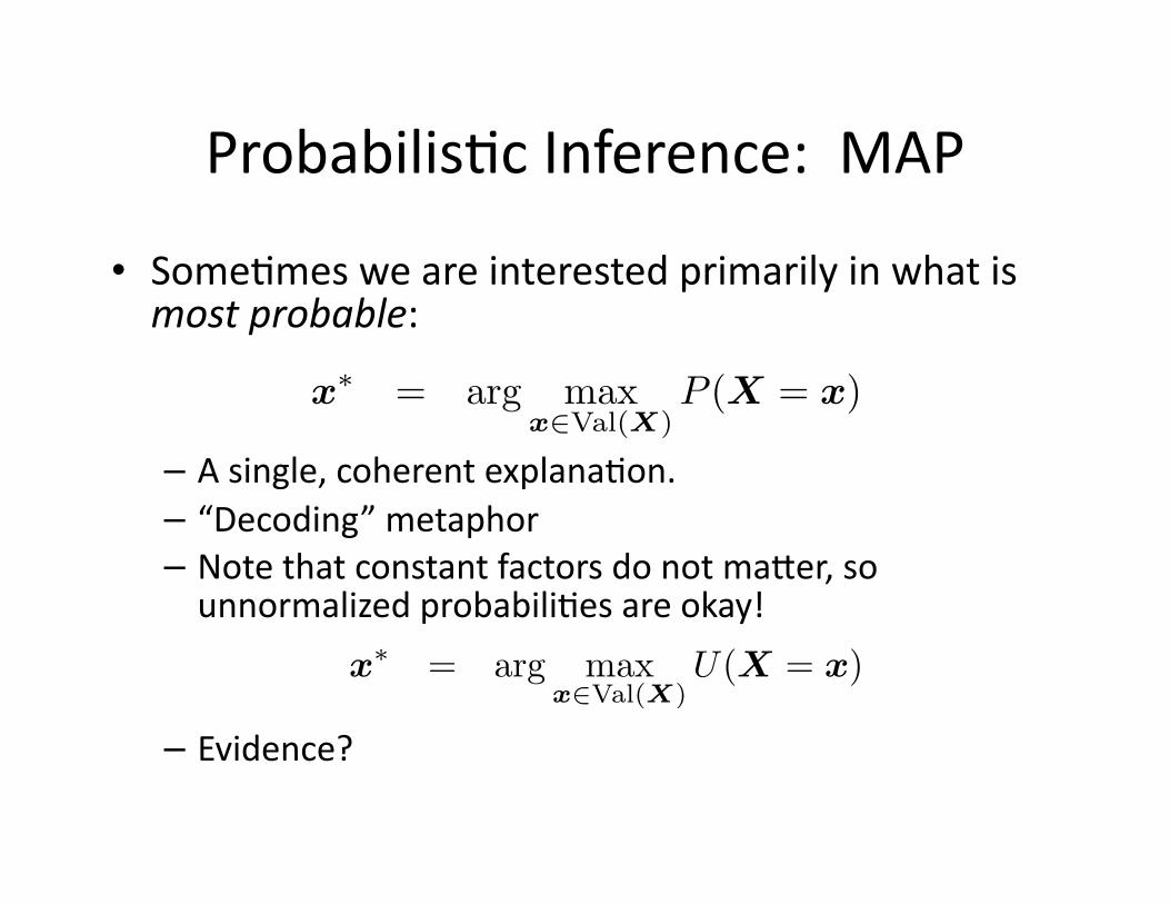
ProbabilisEc Inference: MAP

• SomeEmes we are interested primarily in what is most probable:

– A single, coherent explanaEon.– “Decoding” metaphor– Note that constant factors do not ma]er, so unnormalized probabiliEes are okay!

– Evidence?

x∗ = arg maxx∈Val(X)

P (X = x)


U(X = x)

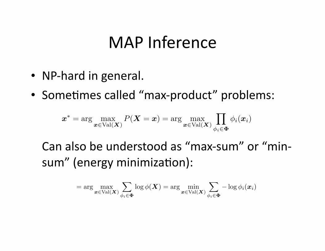
MAP Inference

• NP-‐hard in general.

• SomeEmes called “max-‐product” problems:

Can also be understood as “max-‐sum” or “min-‐sum” (energy minimizaEon):


P (X = x) = arg maxx∈Val(X)

�

φi∈Φ

φi(xi)

= arg maxx∈Val(X)

�

φi∈Φ

log φ(X) = arg minx∈Val(X)

�

φi∈Φ

− log φi(xi)

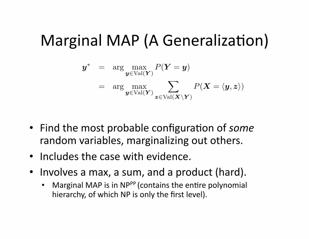
Marginal MAP (A GeneralizaEon)

• Find the most probable configuraEon of some random variables, marginalizing out others.

• Includes the case with evidence.• Involves a max, a sum, and a product (hard).• Marginal MAP is in NPPP (contains the en3re polynomial

hierarchy, of which NP is only the first level).

y∗ = arg maxy∈Val(Y )

P (Y = y)

= arg maxy∈Val(Y )

�

z∈Val(X\Y )

P (X = �y,z�)

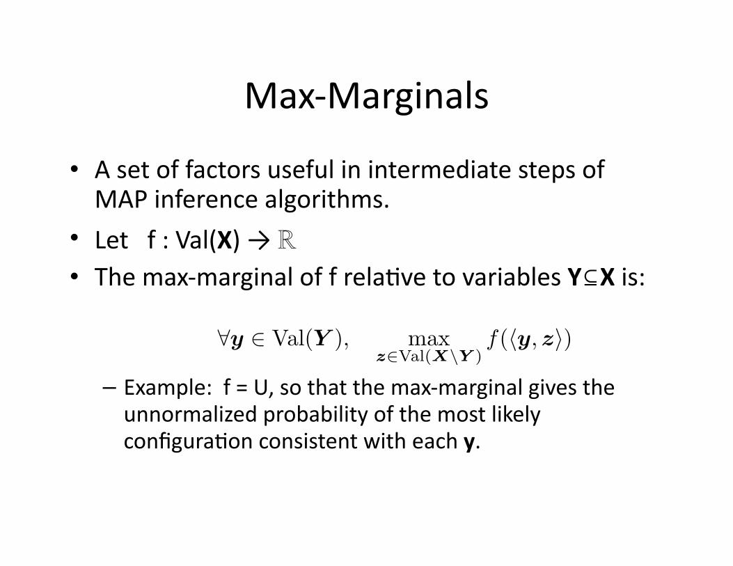
Max-‐Marginals

• A set of factors useful in intermediate steps of MAP inference algorithms.

• Let f : Val(X) → ℝ• The max-‐marginal of f relaEve to variables Y⊆X is:

– Example: f = U, so that the max-‐marginal gives the unnormalized probability of the most likely configuraEon consistent with each y.

∀y ∈ Val(Y ), maxz∈Val(X\Y )

f(�y,z�)

Exact MAP Inference

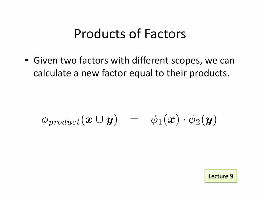
Products of Factors

• Given two factors with different scopes, we can calculate a new factor equal to their products.

φproduct(x ∪ y) = φ1(x) · φ2(y)

Lecture 9

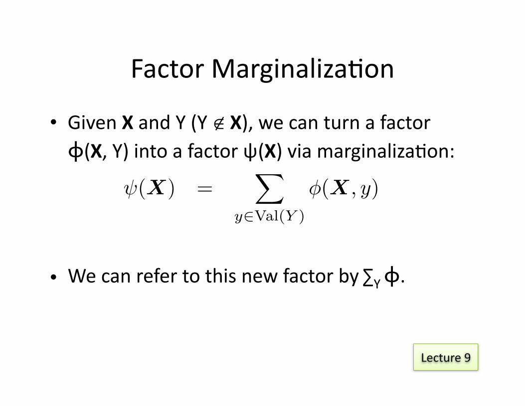
Factor MarginalizaEon

• Given X and Y (Y ∉ X), we can turn a factor ϕ(X, Y) into a factor ψ(X) via marginalizaEon:

• We can refer to this new factor by ∑Y ϕ.

ψ(X) =�

y∈Val(Y )

φ(X, y)

Lecture 9

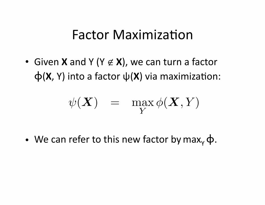
Factor MaximizaEon

• Given X and Y (Y ∉ X), we can turn a factor ϕ(X, Y) into a factor ψ(X) via maximizaEon:

• We can refer to this new factor by maxY ϕ.

ψ(X) = maxY

φ(X, Y )

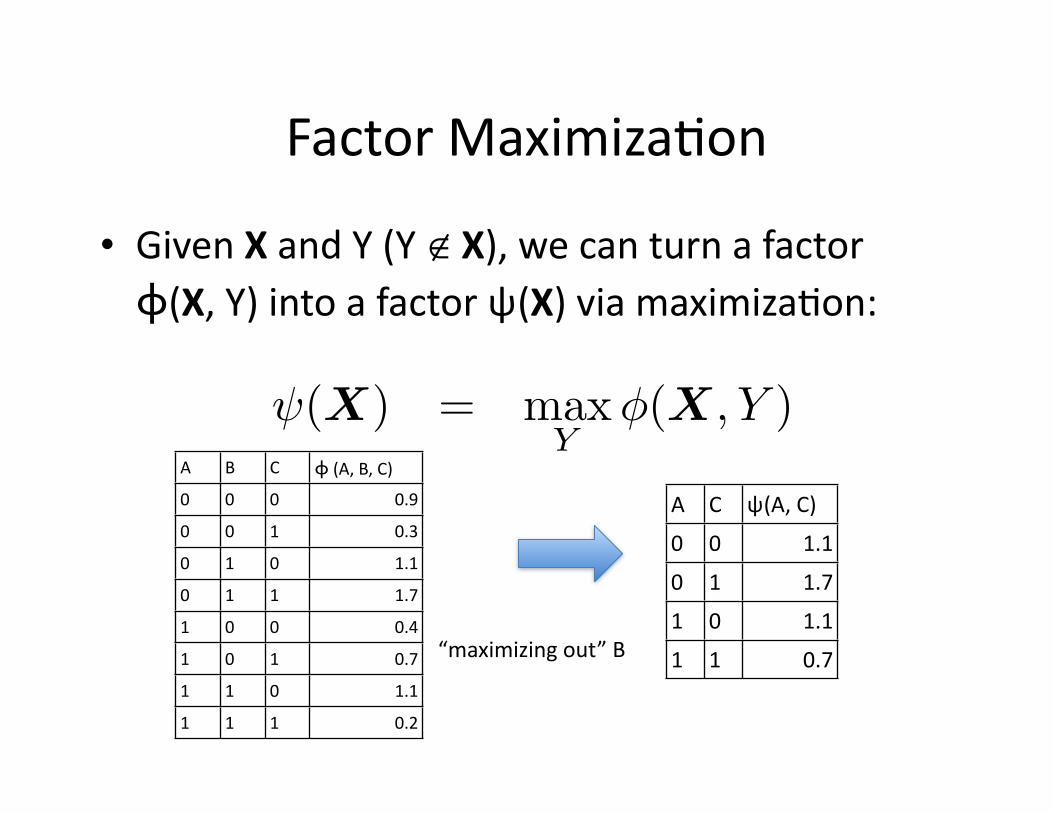
Factor MaximizaEon

• Given X and Y (Y ∉ X), we can turn a factor ϕ(X, Y) into a factor ψ(X) via maximizaEon:

ψ(X) = maxY

φ(X, Y )

A C ψ(A, C)

0 0 1.1

0 1 1.7

1 0 1.1

1 1 0.7“maximizing out” B

A B C ϕ (A, B, C)0 0 0 0.9

0 0 1 0.3

0 1 0 1.1

0 1 1 1.7

1 0 0 0.4

1 0 1 0.7

1 1 0 1.1

1 1 1 0.2

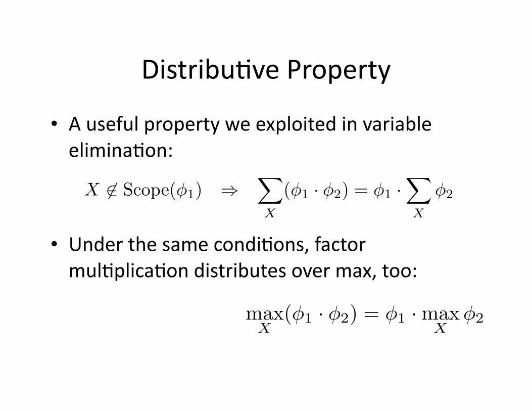
DistribuEve Property

• A useful property we exploited in variable eliminaEon:

• Under the same condiEons, factor mulEplicaEon distributes over max, too:

X �∈ Scope(φ1) ⇒�

X

(φ1 · φ2) = φ1 ·�

X

φ2

maxX

(φ1 · φ2) = φ1 · maxX

φ2

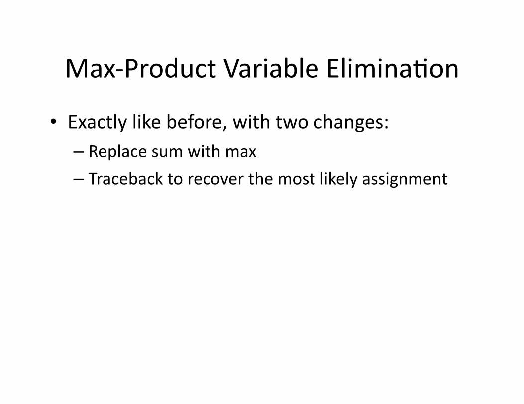
Max-‐Product Variable EliminaEon

• Exactly like before, with two changes:– Replace sum with max

– Traceback to recover the most likely assignment

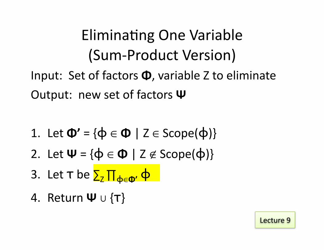
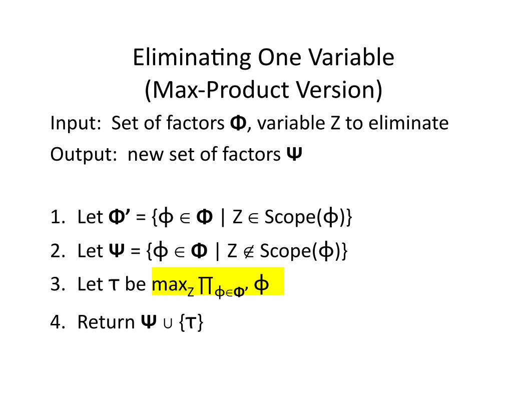
EliminaEng One Variable(Sum-‐Product Version)

Input: Set of factors Φ, variable Z to eliminate

Output: new set of factors Ψ

1. Let Φ’ = {ϕ ∈ Φ | Z ∈ Scope(ϕ)}2. Let Ψ = {ϕ ∈ Φ | Z ∉ Scope(ϕ)}3. Let τ be ∑Z ∏ϕ∈Φ’ ϕ4. Return Ψ ∪ {τ}

Lecture 9

Input: Set of factors Φ, variable Z to eliminate

Output: new set of factors Ψ

1. Let Φ’ = {ϕ ∈ Φ | Z ∈ Scope(ϕ)}2. Let Ψ = {ϕ ∈ Φ | Z ∉ Scope(ϕ)}3. Let τ be maxZ ∏ϕ∈Φ’ ϕ4. Return Ψ ∪ {τ}

EliminaEng One Variable(Max-‐Product Version)

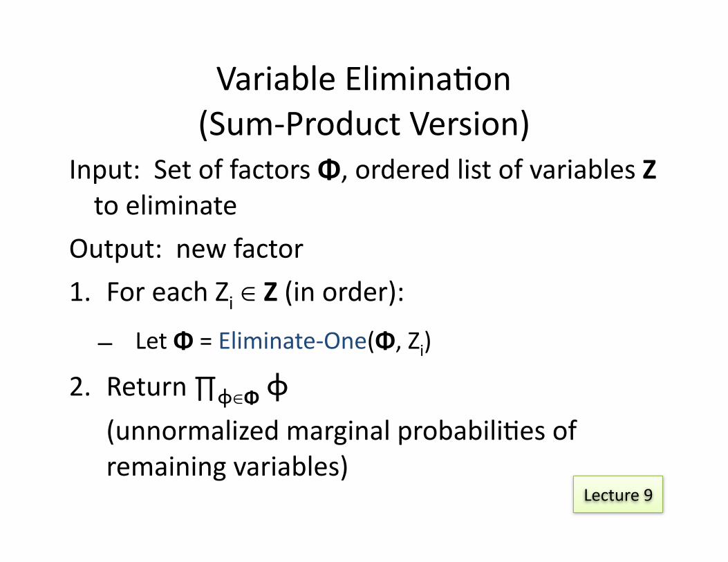
Variable EliminaEon(Sum-‐Product Version)

Input: Set of factors Φ, ordered list of variables Z to eliminate

Output: new factor

1. For each Zi ∈ Z (in order):

– Let Φ = Eliminate-‐One(Φ, Zi)

2. Return ∏ϕ∈Φ ϕ (unnormalized marginal probabiliEes of remaining variables)

Lecture 9

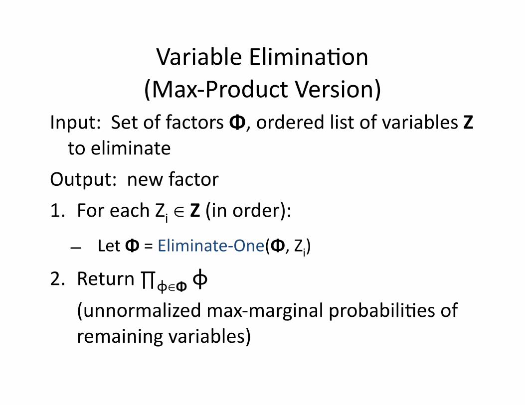
Variable EliminaEon(Max-‐Product Version)


Output: new factor


– Let Φ = Eliminate-‐One(Φ, Zi)

2. Return ∏ϕ∈Φ ϕ (unnormalized max-‐marginal probabiliEes of remaining variables)

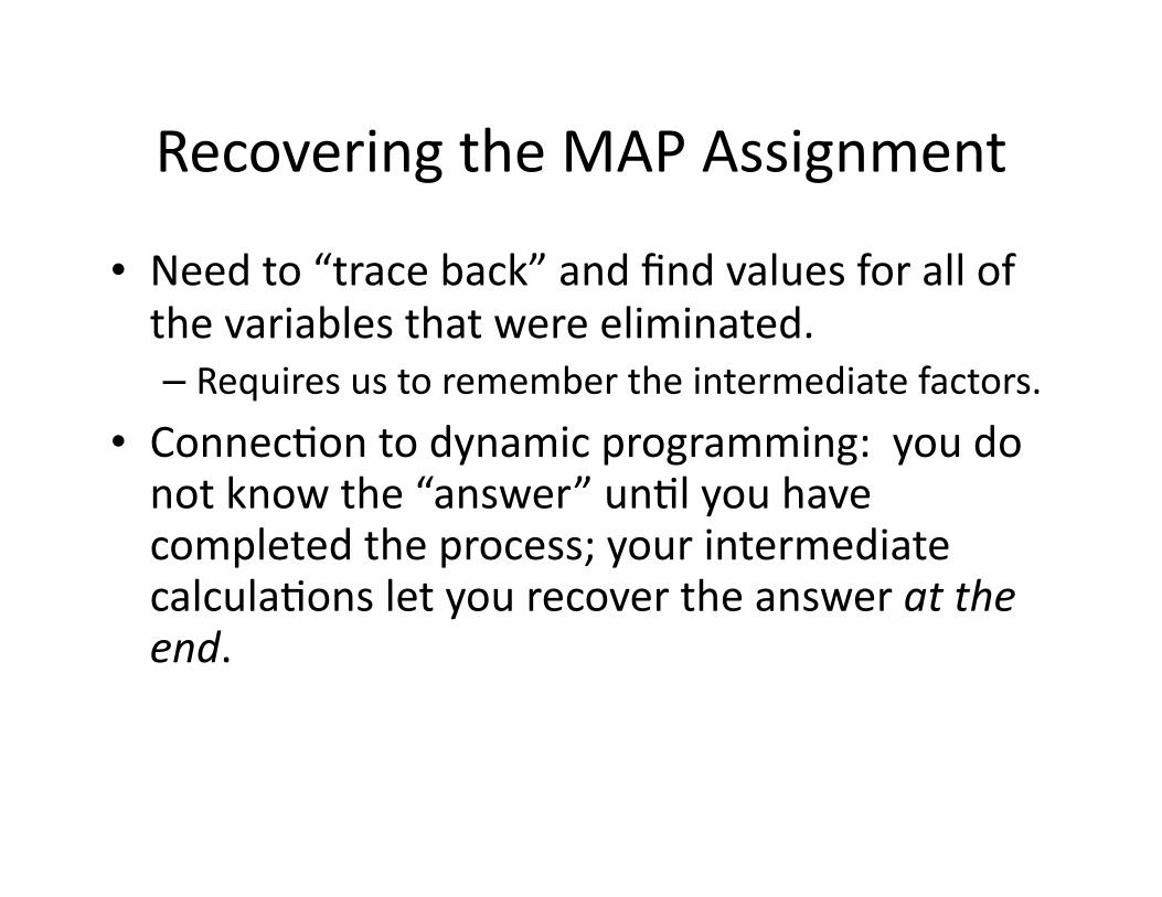
Recovering the MAP Assignment

• Need to “trace back” and find values for all of the variables that were eliminated.– Requires us to remember the intermediate factors.

• ConnecEon to dynamic programming: you do not know the “answer” unEl you have completed the process; your intermediate calculaEons let you recover the answer at the end.

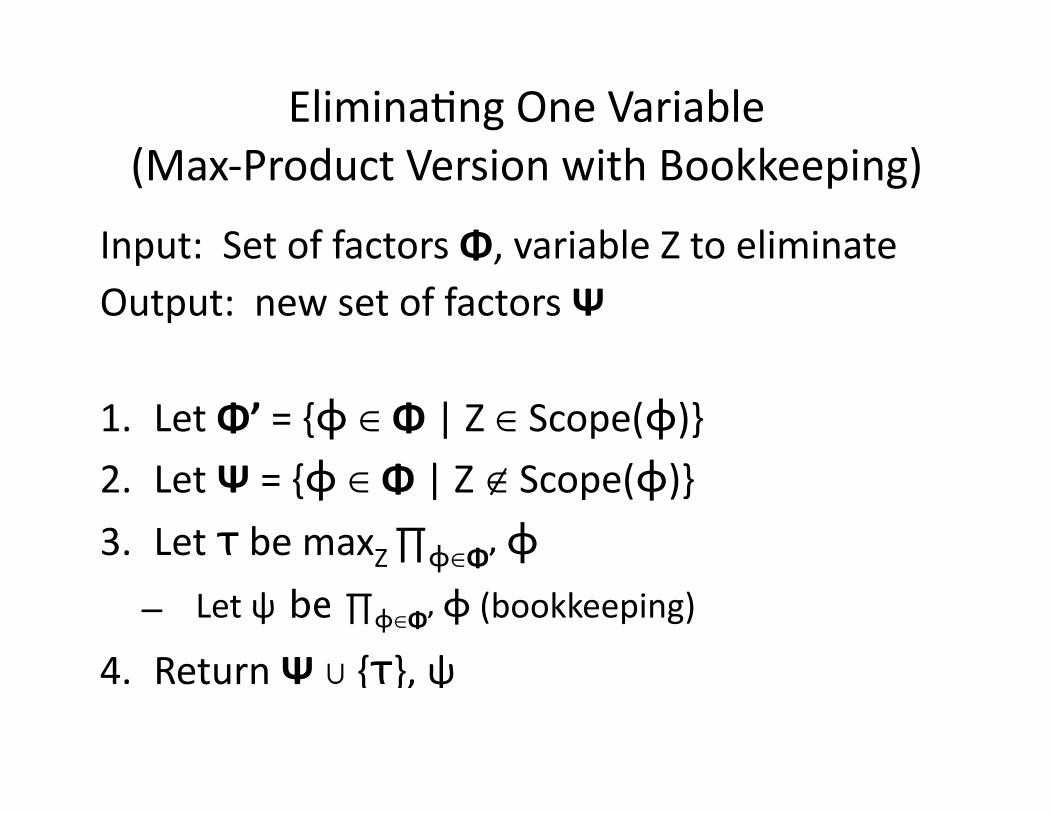
Input: Set of factors Φ, variable Z to eliminateOutput: new set of factors Ψ

1. Let Φ’ = {ϕ ∈ Φ | Z ∈ Scope(ϕ)}2. Let Ψ = {ϕ ∈ Φ | Z ∉ Scope(ϕ)}3. Let τ be maxZ ∏ϕ∈Φ’ ϕ– Let ψ be ∏ϕ∈Φ’ ϕ (bookkeeping)

4. Return Ψ ∪ {τ}, ψ

EliminaEng One Variable(Max-‐Product Version with Bookkeeping)

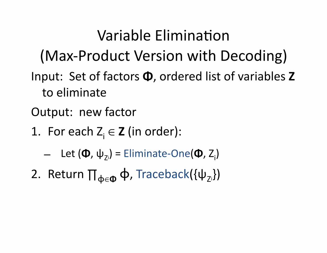
Variable EliminaEon(Max-‐Product Version with Decoding)


Output: new factor


– Let (Φ, ψZi) = Eliminate-‐One(Φ, Zi)

2. Return ∏ϕ∈Φ ϕ, Traceback({ψZi})

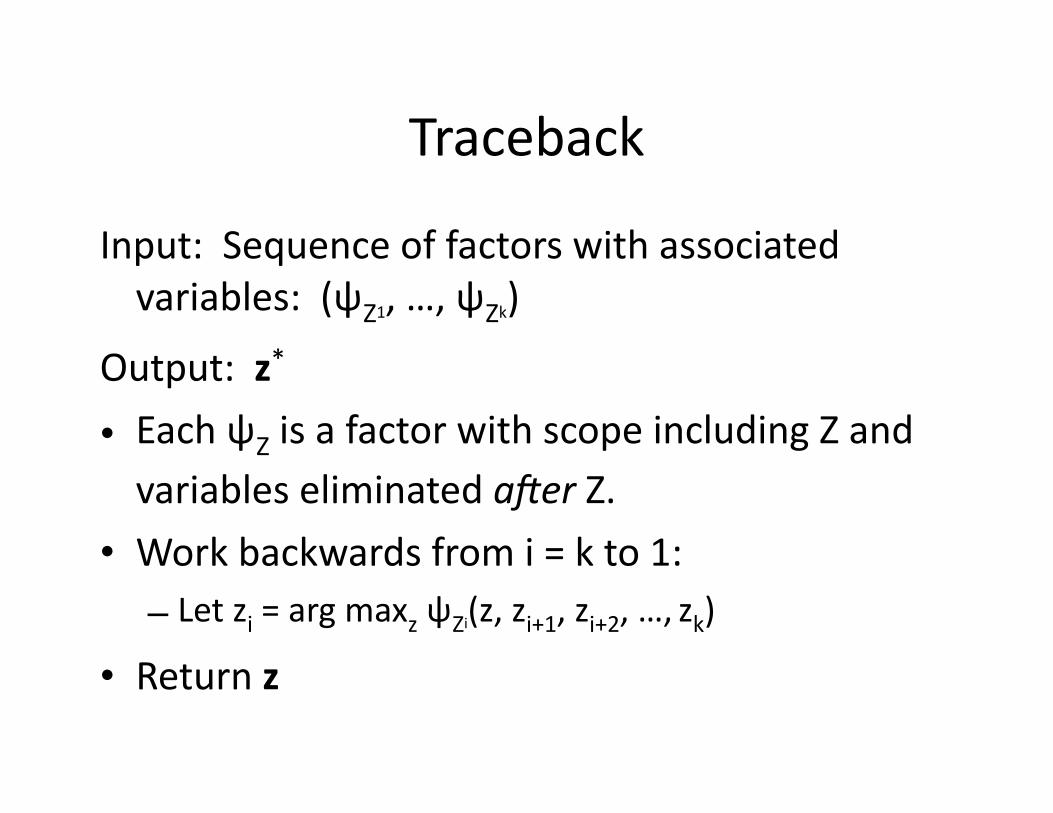
Traceback

Input: Sequence of factors with associated variables: (ψZ1, …, ψZk)

Output: z*

• Each ψZ is a factor with scope including Z and variables eliminated a/er Z.

• Work backwards from i = k to 1:– Let zi = arg maxz ψZi(z, zi+1, zi+2, …, zk)

• Return z

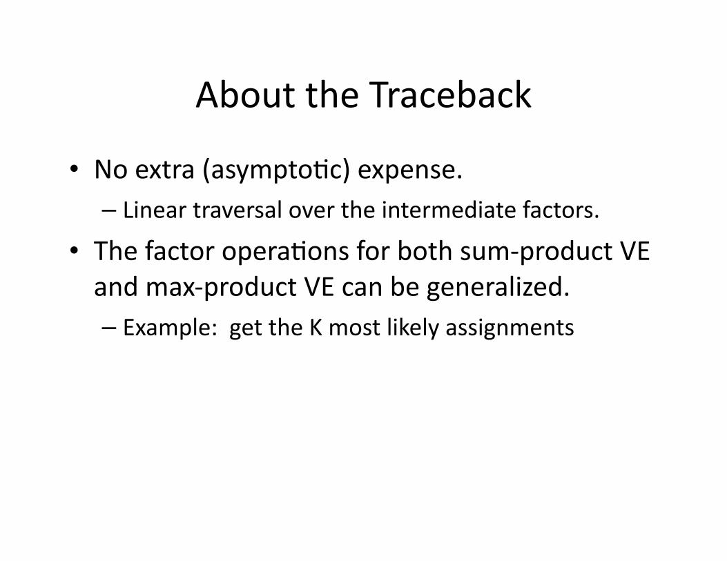
About the Traceback

• No extra (asymptoEc) expense.– Linear traversal over the intermediate factors.

• The factor operaEons for both sum-‐product VE and max-‐product VE can be generalized.– Example: get the K most likely assignments

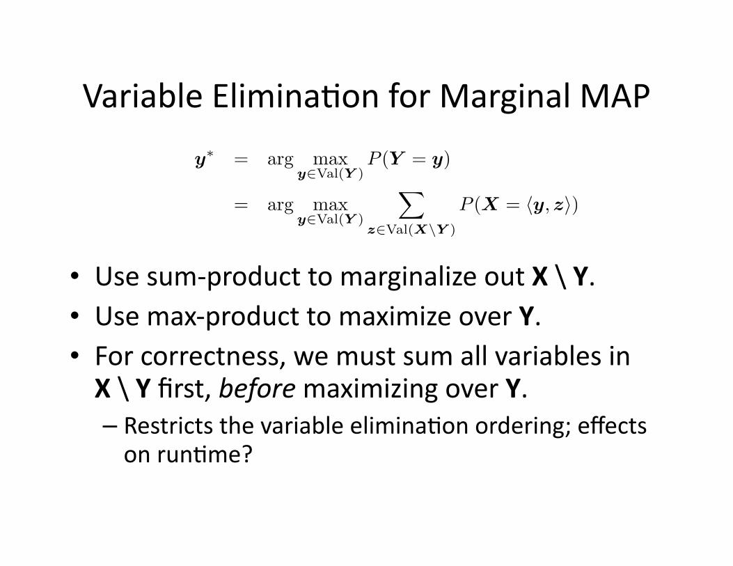
Variable EliminaEon for Marginal MAP

• Use sum-‐product to marginalize out X \ Y.• Use max-‐product to maximize over Y.• For correctness, we must sum all variables in X \ Y first, before maximizing over Y.– Restricts the variable eliminaEon ordering; effects on runEme?

y∗ = arg maxy∈Val(Y )

P (Y = y)

= arg maxy∈Val(Y )

�

z∈Val(X\Y )

P (X = �y,z�)

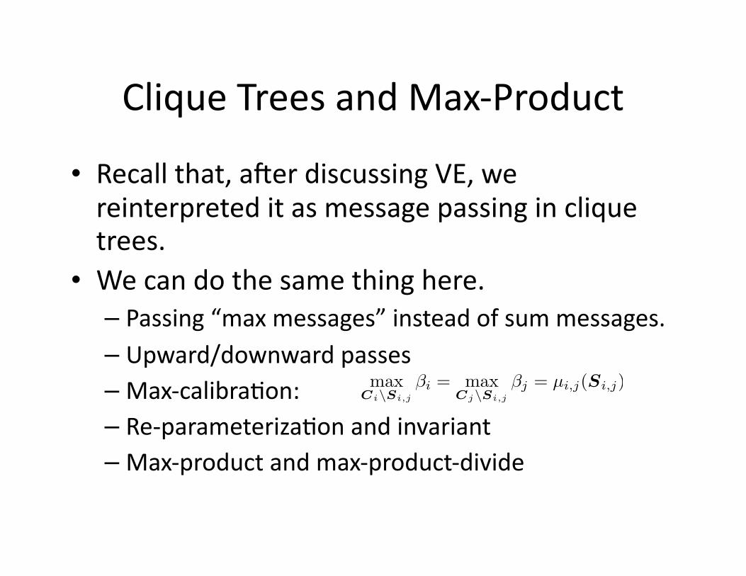
Clique Trees and Max-‐Product

• Recall that, awer discussing VE, we reinterpreted it as message passing in clique trees.

• We can do the same thing here.– Passing “max messages” instead of sum messages.– Upward/downward passes–Max-‐calibraEon:– Re-‐parameterizaEon and invariant–Max-‐product and max-‐product-‐divide

maxCi\Si,j

βi = maxCj\Si,j

βj = µi,j(Si,j)


• How to decode?

• Choose value of each random variable based on local beliefs?


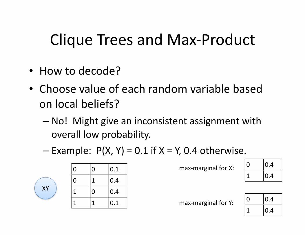
• How to decode?

• Choose value of each random variable based on local beliefs?– No! Might give an inconsistent assignment with overall low probability.

– Example: P(X, Y) = 0.1 if X = Y, 0.4 otherwise.

XY

0 0 0.1

0 1 0.4

1 0 0.4

1 1 0.1

0 0.4

1 0.4

0 0.4

1 0.4

max-‐marginal for X:

max-‐marginal for Y:


• How to decode?

• Choose value of each random variable based on local beliefs?– This is okay if the calibrated node beliefs are unambiguous (no Ees).


• Local opEmality of a (complete) configuraEon:

• Local opEmality is saEsfied for all clique tree node beliefs if and only if x is globally opEmal (global MAP configuraEon).– Use a traceback to get a consistent assignment that is locally opEmal everywhere.

x[Ci] ∈ arg maxci

βi(ci)

Exact MAP

• SomeEmes you can do it.

• Owen, the structure of your problem gives you a specialized algorithm.– Examples I have seen: dynamic programming (really just VE); maximum weighted biparEte matching, minimum spanning tree, max flow, …

Approximate MAP Inference

Approximate MAP Inference

• Huge topic, ge|ng a lot of a]enEon.

• Key techniques:–Max-‐product belief propagaEon in loopy cluster graphs

– Linear programming formulaEons

Max-‐Product Belief PropagaEonin Loopy Cluster Graphs

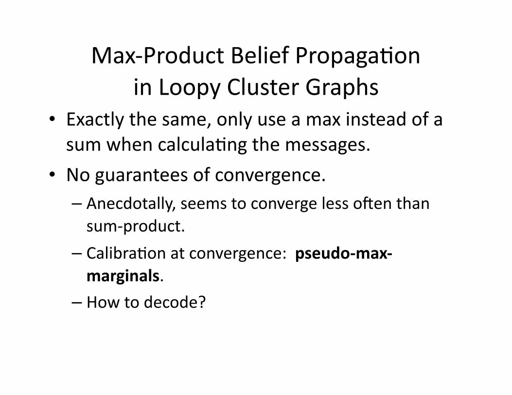
• Exactly the same, only use a max instead of a sum when calculaEng the messages.

• No guarantees of convergence.– Anecdotally, seems to converge less owen than sum-‐product.

– CalibraEon at convergence: pseudo-‐max-‐marginals.

– How to decode?

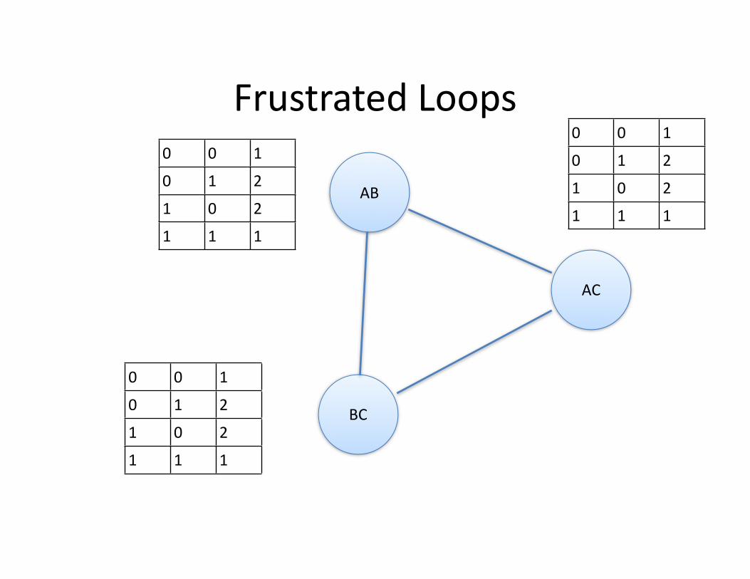
Frustrated Loops

AB

BC

AC

0 0 1

0 1 2

1 0 2

1 1 1

0 0 1

0 1 2

1 0 2

1 1 1

0 0 1

0 1 2

1 0 2

1 1 1

Max-‐Product Belief PropagaEonin Loopy Cluster Graphs: Decoding

• When all node beliefs are unambiguous (no Ees), there is a unique maximizing assignment to the local clusters that is consistent.

• It’s possible to have ambiguous node beliefs and a locally opEmal joint assignment!

• In general, finding the locally opEmal assignments that are consistent is a constraint sa;sfac;on problem.– NP hard.

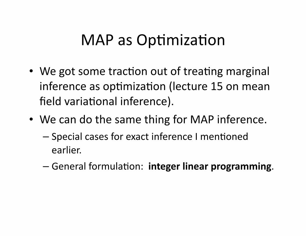
MAP as OpEmizaEon

• We got some tracEon out of treaEng marginal inference as opEmizaEon (lecture 15 on mean field variaEonal inference).

• We can do the same thing for MAP inference.– Special cases for exact inference I menEoned earlier.

– General formulaEon: integer linear programming.

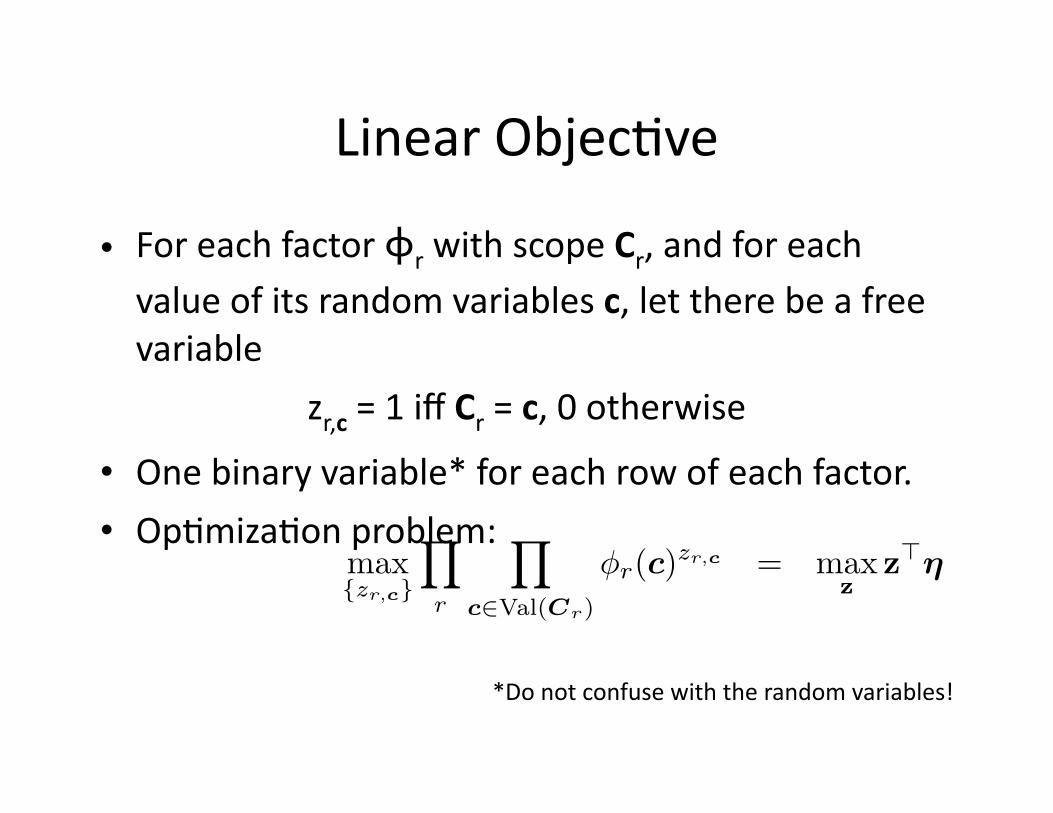
Linear ObjecEve

• For each factor ϕr with scope Cr, and for each value of its random variables c, let there be a free variable

zr,c = 1 iff Cr = c, 0 otherwise

• One binary variable* for each row of each factor.

• OpEmizaEon problem:

*Do not confuse with the random variables!

max{zr,c}

�

r

�

c∈Val(Cr)

φr(c)zr,c = maxz

z�η

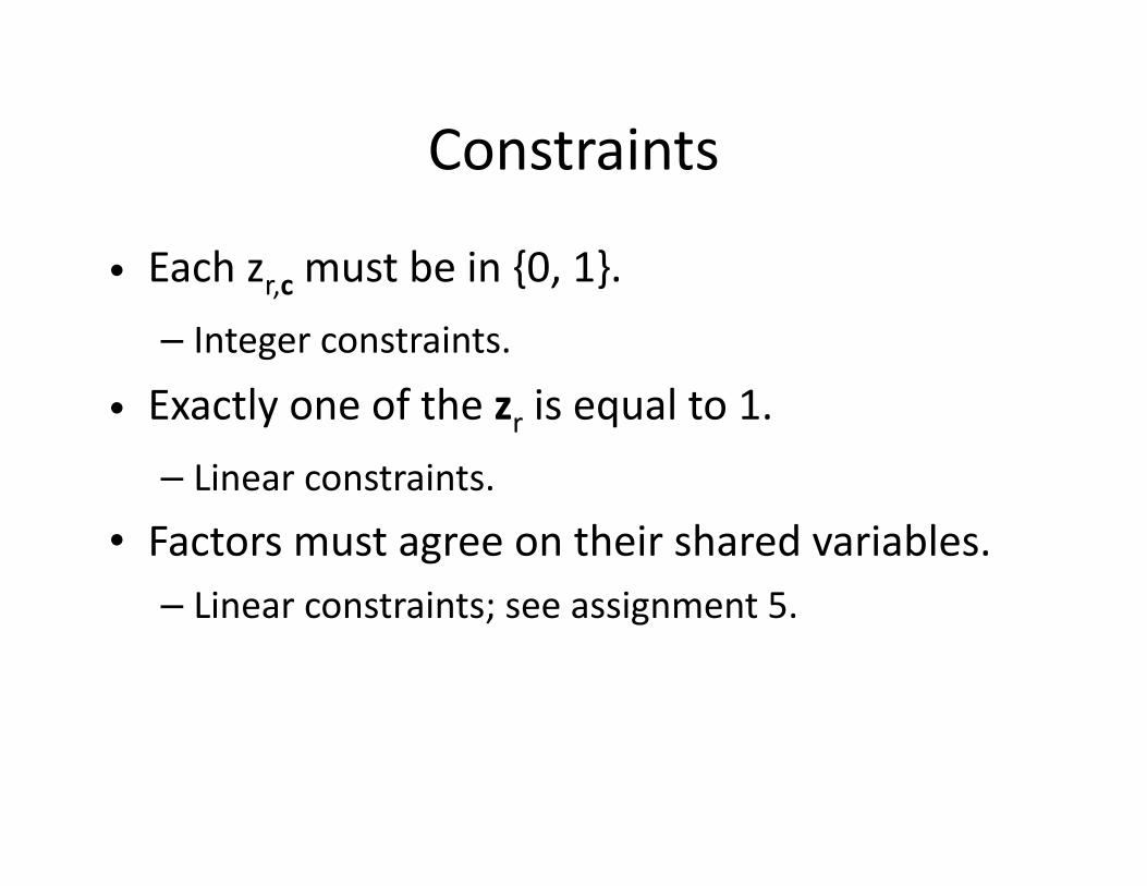
Constraints

• Each zr,c must be in {0, 1}.

– Integer constraints.

• Exactly one of the zr is equal to 1.

– Linear constraints.• Factors must agree on their shared variables.– Linear constraints; see assignment 5.

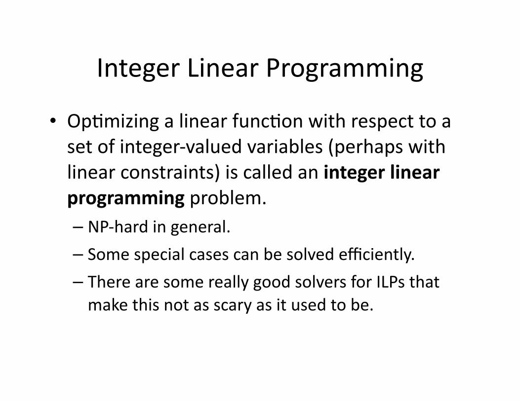
Integer Linear Programming

• OpEmizing a linear funcEon with respect to a set of integer-‐valued variables (perhaps with linear constraints) is called an integer linear programming problem.– NP-‐hard in general.– Some special cases can be solved efficiently.

– There are some really good solvers for ILPs that make this not as scary as it used to be.

RelaxaEon

• Relaxing the integer constraints from {0, 1} to [0, 1] has useful effects:– ILP becomes an LP; solvable in polynomial Eme.

– Feasible region of the LP is a polytope.– Solve the relaxed LP; if soluEon is integer, you are done. If not, go greedy, randomized rounding, etc.

• Can add more constraints to the LP, perhaps ge|ng a be]er approximaEon.

General Solvers

• General solvers are always tempEng, but algorithms that “know” about the special structure of your problem are usually faster and/or more accurate.

• My advice: formulate the problem first, understand the landscape of specialized opEmizaEon techniques that might apply, and resort to general techniques if you can’t find anything.– And be on the lookout for ways to improve the general technique using your problem’s structure!

Final Note

• Finding the best consistent configuraEon is an old problem; old soluEons exist.– Branch and bound, A*– Local search methods (e.g., beam search, tabu)– Randomized methods (e.g., simulated annealing)

• Some of the above can be be]er understood or generalized using data structures developed for inference (e.g., clique trees and cluster graphs).

Documents

Graphical)Models - UMass Amherst