Graphing linear functions 572 Drawing a logarithmic graph

... __

.y :~><~!: ~ :f t.1?{;::r,.,' -:: '<:' X - , V

~ ,.,,k_:;vr

-;! ·using a graphic display calculator

I ..J .J This chapter shows you how to use your graphic display calculator (GDC) to solve the different types of problems that you will meet in your course. You should not work through the whole of the chapter - it is simply here for reference purposes. When you are working on problems in the mathematical chapters, you can refer to this chapter for extra help with your GDC if you need it.

GDC instructions on CD: The instructions in this chapter are for the TI-Nspire made/. Instructions for the same techniques using the T/-84 Plus and the Casio FX-9860GI/ are

Chapter contents 1 Functions

1.1 Graphing linear functions .. ... ...... ... ... 572 Finding information about the graph

1.2 Finding a zero ....... ......... ... .... .. ... ........... .. 572 1.3 Finding the gradient

(slope) of a line .... .. ... ... .. ... ...... ... .. .... ....... 573 Simultaneous equations 1.4 Solving simultaneous

equations graphically ... .. ..... .. ... .. .......... 574 1.5 Solving simultaneous

linear equations .............................. ......... 576 Quadratic functions 1.6 Drawing a quadratic

graph ....... ...... .. ......... .. ...... .. .... ... ....... .... ..... ... 577 1.7 Solving quadratic equations .............. 578 1.8 Finding a local minimum

or maximum point ....... .. ....... .. ... ............ 579 Exponential functions 1.9 Drawing an exponential

graph .. .. ........ .. .. ....... .. ... .. .......... .. ..... ... .......... 583 1.10 Finding a horizontal

asymptote ....... ................. ........................... 584

~ Using a graphic display calculator

available on the CD.

Logarithmic functions 1.11 Evaluating logarithms ................ .......... 585 1.12 Finding an inverse function ............ ... 585 1.13 Drawing a logarithmic graph ..... .. .... 588 Trigonometric functions 1.14 Degrees and radians .......... ....... ............ 589 1.15 Drawing trigonometric

graphs ...... .. .... ... ....... ......... ..... ......... .. ... ........ 590 More complicated functions 1.16 Solving a combined quadratic and

exponential equation ......... ......... .......... 591 Modeling 1.17 Using sinusoidal regression ...... ... ... ... 592 1.18 Using transformations to

model a quadratic function ...... ... ...... 594 1.19 Using sliders to model an

exponential function ..... ... .. ..... ......... ..... 596 2 Differential calculus

Finding gradients, tangents and maximum and minimum points 2.1 Finding the gradient at a point .... .... 598 2.2 Drawing a tangent to a curve .... .. ..... 599

2.3 Finding maximum and

minimum points .................................. ... 600 Derivatives 2.4 Finding a numerical derivative ............ ... 602 2.5 Graphing a numerical

derivative ......................... ..... .... ... ... .......... .. 603 2.6 Using the second derivative .............. 605

3 Integral calculus 3.1 Finding the value of an

indefinite integral ........... ............... ... .. .... 606 3.2 Finding the area under a curve ........ 607

4 Vectors 4.1 Calculating a scalar product ............. 608 4.2 Calculating the angle between

two vectors ....... ......................................... 610 5 Statistics and probability

Entering data 5.1 Entering lists of data ............................ 612 5.2 Entering data from a

frequency table .................... .. .................. 612 Drawing charts 5.3 Drawing a frequency

histogram from a list ............................ 613 5.4 Drawing a frequency histogram

from a frequency table ......................... 614

Before you start You should know:

5.5 Drawing a box and whisker

diagram from a list ................................ 614 5.6 Drawing a box and whisker

diagram from a frequency table .. .... 616 Calculating statistics 5.7 Calculating statistics from a list ...... 617 5.8 Calculating statistics

from a frequency table ...................... ... 618 5.9 Calculating the interquartile

range ............................................................. 619 5.10 Using statistics ......................................... 620 Calculating binomial probabilities

5.11 Use of nCr .... ............................................. 621 5.12 Calculating binomial probabilities ............ 622 Calculating normal probabilities 5.13 Calculating normal probabilities

from X-values ........................................... 624 5.14 Calculating X-values

from normal probabilities .... .. ...... .... .. 625 Scatter diagrams, linear regression and the correlation coefficient 5.15 Scatter diagrams using a

Data & Statistics page .......................... 627 5.16 Scatter diagrams using a

Graphs page .............................................. 629

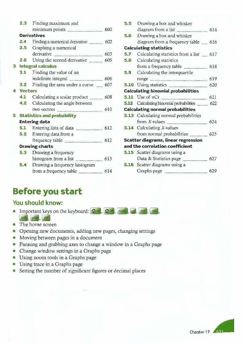
• Opening new documents, adding new pages, changing settings • Moving between pages in a document • Panning and grabbing axes to change a window in a Graphs page • Change window settings in a Graphs page • Using zoom tools in a Graphs page • Using trace in a Graphs page • Setting the number of significant figures or decimal places

Chaoter 17

1 Functions 1.1 Graphing linear functions

Example 1

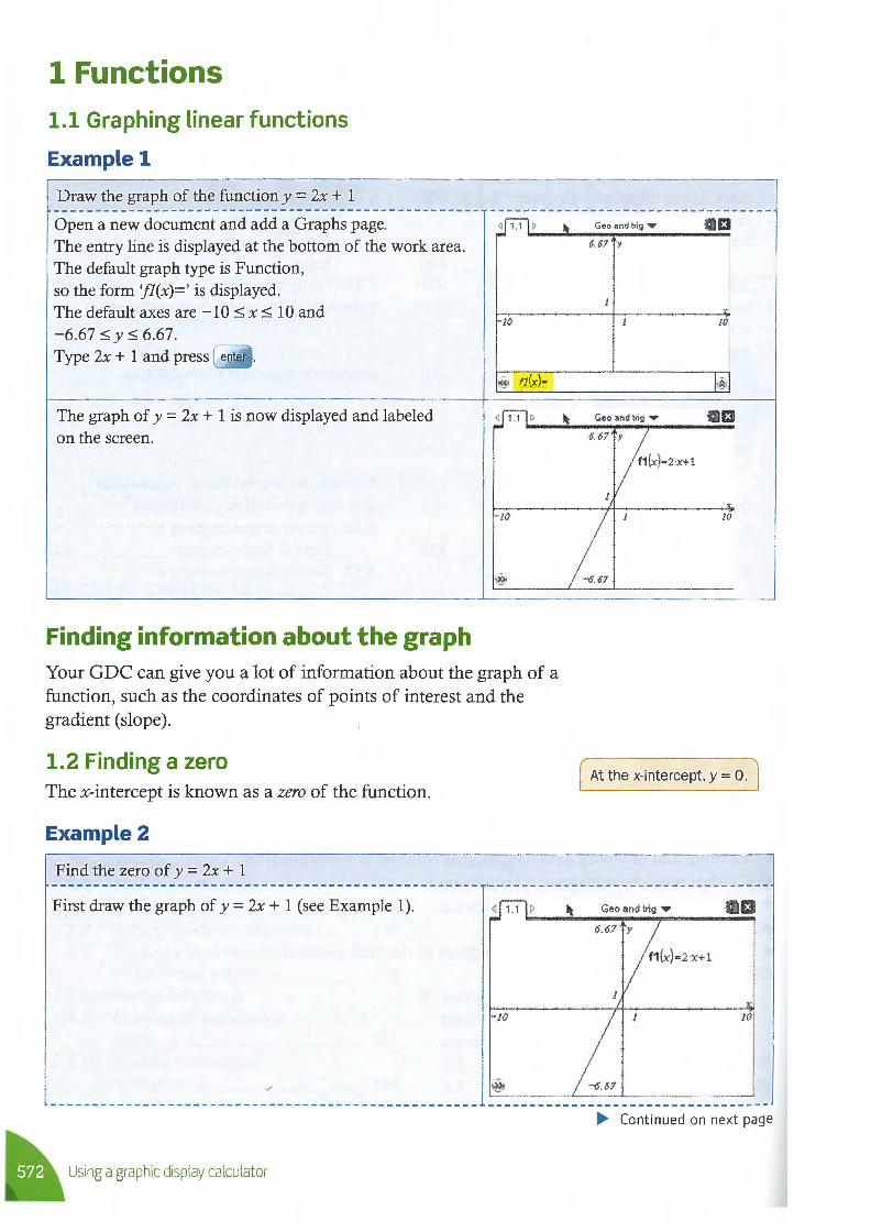
Draw the graph of the function y = 2x + 1

Open a new document and add a Graphs page. < 1. 1 > Geo and trig ..,. £1 The entry line is displayed at the bottom of the work area. The default graph type is Function, so the form 'fl(x)=' is displayed. The default axes are -10 $ x $ l O and -6.67:::; y s 6.67.

The graph of y = 2x + 1 is now displayed and labeled on the screen.

Finding information about the graph

-JO

- JO

Your GDC can give you a lot of information about the graph of a function, such as the coordinates of points of interest and the gradient (slope).

1.2 Finding a zero The x-intercept is known as a zero of the function.

Example 2

Find the zero of y = 2x + 1

First draw the graph of y = 2x + 1 (see Example 1).

-JO

~ U~ng a graphic display calculator

6.67 y

10

~ Geo and trig ..,. ma 6.67 y

f1 (x)=2 x+ l

10

- 6.67

( At the x-intercept, y = 0. j

~ Geo and trig 'Y El 6.67 y

f1 (x)=2 ·x+ 1

10

-6.67

• Continued on next page

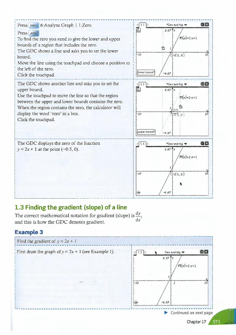
Press menu 6:Analyze Graph I 1 :Zero

Press enter

To find the zero you need to give the lower and upper bounds of a region that includes the zero. The G DC shows a line and asks you to set the lower bound. Move the line using the touchpad and choose a position to the left of the zero. Click the touchpad.

The GDC shows another line and asks you to set the upper bound.

- JO

jtowe r bound]

*Geo and trig ..,. £1

JO

*Geo and trig ,.. £1 6.67 Y

f 1(x)=2 ·x+ 1 Use the touch pad to move the line so that the region between the upper and lower bounds contains the zero. When the region contains the zero, the calculator will display the word 'zero' in a box. -------zero>-+-.- - - - -

\ . Jo) -JO 10

Click the touchpad.

1jupper bound] , _6_ 67

The GDC displays the zero of the function y = 2x +lat the point (-0.5, 0).

1.3 Finding the gradient (slope) of a line

- JO

>

The correct mathematical notation for gradient (slope) is dy ,

and this is how the GDC denotes gradient. dx

Example 3

Find the gradient of y = 2x + l

First draw the graph of y = 2x + l (see Example 1).

- JO

>

*Geo a nd trig ,.. £1

JO

-6.67

£1

f1 (x)=2·x+ 1

JO

- 6.67

• Chapter 17

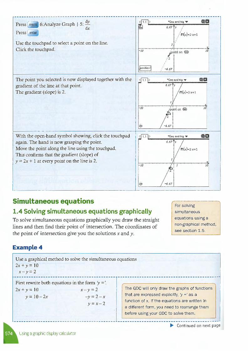
Press

Press

6:Analyze Graph I 5: dy d.x

Use the touch pad to select a point on the line. Click the touchpad. -JO

*Geo and trig ..,.

6.67 y

,/f1 (x)=2 ·x+l

jpointon (§)

/2

£1

1jposition] -6. 67

The point you selected is now displayed together with the gradient of the line at that point. The gradient (slope) is 2.

With the open-hand symbol showing, click the touchpad again. The hand is now grasping the point. Move the point along the line using the touchpad. This confirms that the gradient (slope) of y = 2x + 1 at every point on the line is 2.

Simultaneous equations

-JO

-JO

>

1.4 Solving simultaneous equations graphically To solve simultaneous equations graphically you draw the straight lines and then find their point of intersection. The coordinates of the point of intersection give you the solutions x and y.

Example4

Use a graphical method to solve the simultaneous equations 2x + y = 10 x-y=2

First rewrite both equations in the form '.Y = '.

*Geo and trig ..,. £1

10

*Geo and trig ..,. £1 6.67 y

-6.67

f1(x)=2 ·x+l

10

For solving

simultaneous

equations using a

non-graphical method,

see section 1.5.

2x+y=10 x-y=2

y=10-2x -y=2 -x

y=x-2

The GDC will only draw the graphs of functions

that are expressed explicitly, 'y = ' as a

function of x. If the equations are written in


a different form, you need to rearrange them

before using your GDC to solve them.


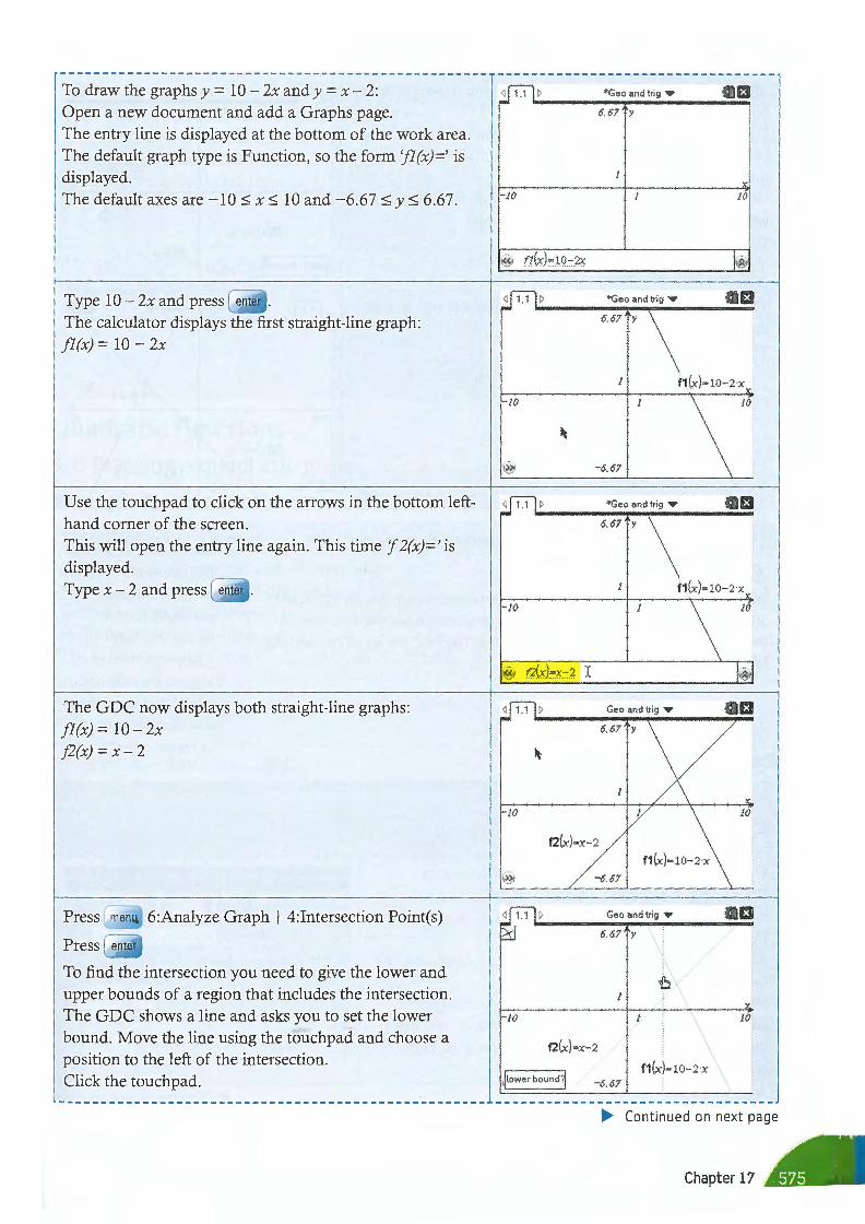
To draw the graphs y = I0-2x andy = x -2: Open a new document and add a Graphs page. The entry line is displayed at the bottom of the work area. The default graph type is Function, so the form 'fl (x)=' is displayed. The default axes are -10 ~ x ~ IO and -6.67 ~ y ~ 6.67.

Type 10 - 2x and press enter .

The calculator displays the first straight-line graph: fl(x) = IO - 2x

Use the touch pad to click on the arrows in the bottom lefthand corner of the screen. This will open the entry line again. This time J 2(x)=' is displayed.

The GDC now displays both straight-line graphs: Jl(x) = IO- 2x j2(x) = x-2

Press

Press

6:Analyze Graph I 4:Intersection Point(s)

To find the intersection you need to give the lower and upper bounds of a region that includes the intersection. The GDC shows a line and asks you to set the lower bound. Move the line using the touchpad and choose a position to the left of the intersection. Click the touchpad.

-*Geo and trig ..,. El

6.67 y

-JO

*Geo and trig ""'

6.67 y

f1 (x)=l0- 2-x

-10 10

- 6.67

*Geo and trig ""' El 6.67 y

f1(x)=l0-2-x

-JO 10

~• f2{x):=x-2. I

Geo and trig •

6.67 y

- 10 10

f1 (x)=l0-2-x - 6.67

Geo and trig ""' El 6.67 y

- JO JO

f2(x) =x- 2

f1 (x)=l0-2-x -6.67


Chapter 17

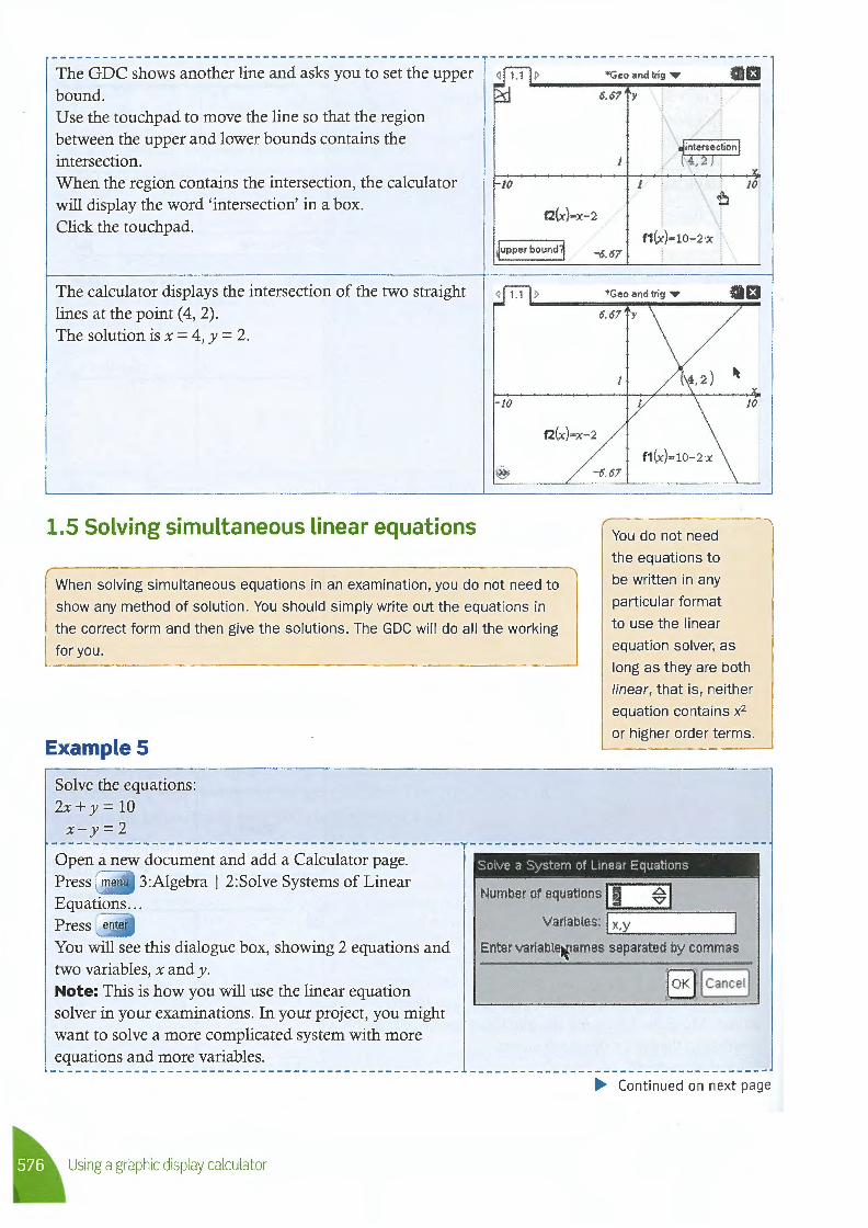
The GDC shows another line and asks you to set the upper bound. Use the touch pad to move the line so that the region between the upper and lower bounds contains the intersection. When the region contains the intersection, the calculator will display the word 'intersection' in a box. Click the touchpad.

The calculator displays the intersection of the two straight lines at the point (4, 2). The solution is x = 4, y = 2.

1.5 Solving simultaneous linear equations

*Geo and trig ..,.

6.67 Y

JO

f2(x) =x- 2

Cll3

intersection 4,

Jupper bound3 -6.67 f1(x)•10-2·x !

*Geo and trig • 13 6.67 y

- JO 10

f2 (x)=x- 2

f1(x)= 10-2x i -6.67

You do not need

the equations to

When solving simultaneous equations in an examination, you do not need to

show any method of solution. You should simply write out the equations in

the correct form and then give the solutions. The GDC will do all the working

for you.

be written in any

particular format

to use the linear

equation solver, as

long as they are both

linear, that is, neither

equation contains x2

or higher order terms. Example 5

Solve the equations: 2x+ y = 10 x-y=2

Open a new document and add a Calculator page. Press menu 3:Algebra I 2:Solve Systems of Linear Equations ... Press enter

You will see this dialogue box, showing 2 equations and two variables, x and y. Note: This is how you will use the linear equation solver in your examinations. In your project, you might want to solve a more complicated system with more equations and more variables.

Using a graphic display calculator

Solve a System of Linear Equations

Number of equations I m ~ I Variables: l~x~,y _____ ~

Enter variabletames separated by commas

I OK) I Cancetj

• Continued on next pa ge

Press enter and you will see the template on the right. Type the two equations into the template, using the arrow keys .... .,,- to move within the template. Press enter and the GDC will solve the equations, giving the solutions in the form {x, y}.

The solutions are x = 4, y = 2.

Quadratic functions 1.6 Drawing a quadratic graph

Example 6

Num Alg 1 "I'

linSolve( ff: , {x,y})

< 1 .1 > Num Alg 1 "I' ~

({2-x+y=l0 { }) linSolve , x,y x-y=2

{ 4,2}

El !?SJ

I

I I

I

I

El

Draw the graph of y = :x!- - 2x + 3 and display using suitable axes.

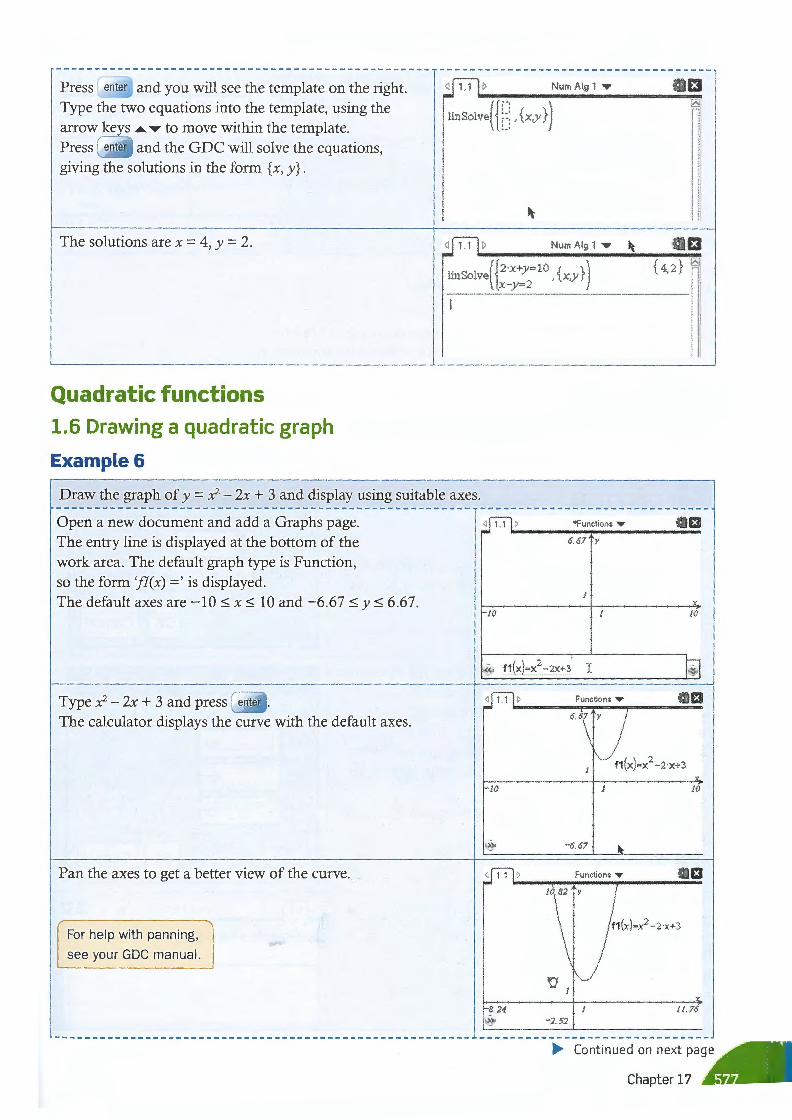
Open a new document and add a Graphs page. The entry line is displayed at the bottom of the work area. The default graph type is Function, so the form 'fl(x) =' is displayed. The default axes are -10 ~ x ~ IO and -6.67 ~ y ~ 6.67.

Type :x!- - 2x + 3 and press enter .

The calculator displays the curve with the default axes.

Pan the axes to get a better view of the curve.

For help with panning,

see your GDC manual.

-JO

- JO

- 8. 24 >

*Functions • £1 6.67 y

10

X

Functions ..,

6.67 y

f1 (x)-x2 -2 x+3

10

-6.67

Functions .., £1 JO. 82 y

11.76 -2. 52


Chapter 17

Grab the x-axis and change it to make the quadratic curve fit the screen better.

•Functions ,..

10.82 y

13

For help with changing

axes, see your GDC

manual. f1(x)=x2- 2·x+3

-2. 52

1.7 Solving quadratic equations

When solving quadratic equations in an examination, you do not need to

show any method of solution. You should simply write out the equations in

the correct form and then give the solutions. The GDC_ will do all the working

for you.

Example 7

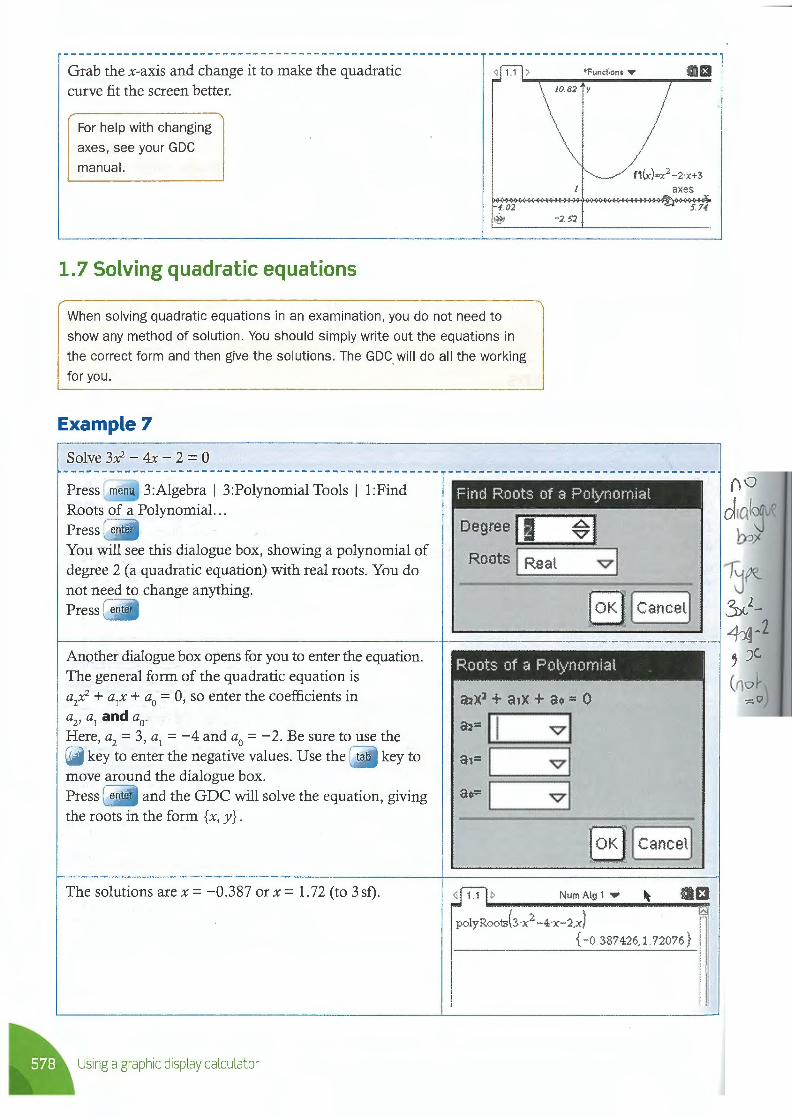
Solve 3x2 - 4x - 2 = 0

Press menu 3:Algebra I 3:Polynomial Tools I 1:Find Roots of a Polynomial. .. Press enter

You will see this dialogue box, showing a polynomial of degree 2 (a quadratic equation) with real roots. You do not need to change anything.

I

Find Roots of a Poly·nomial

Degree I a ~, Roots I Real vi

[OK) [ Cancel}

f-----------------------+------------------, Another dialogue box opens for you to enter the equation. The general form of the quadratic equation is a

2x2 + a

1x + a

0 = 0, so enter the coefficients in

a2

, a1 and a0

.

Here, a2 = 3, a

1 = -4 and a

0 = -2. Be sure to use the

(-) key to enter the negative values. Use the tab key to move around the dialogue box. Press enter and the GDC will solve the equation, giving the roots in the form {x, y} .

The solutions are x = -0.387 or x = l. 72 (to 3 sf).


Roots of a Polynomial

a2= I I vi a,=~,;:::: :_ ===-v:_,- I ao= I vi -----

NumAlg 1 • \

poly Rootsb ·x2 -4-x- 2,x)

{ - 0.387426,1.72076}

no d1ol~\/

OJ)(

18~ 3><-2_ 4-x -2 5 JC

(no~ :;:::\J)

1.8 Finding a local minimum or maximum point

Example 8

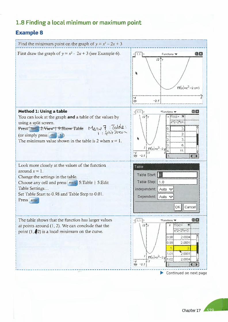
Find the minimum point on the graph of y = :x2 - 2x + 3

First draw the graph of y = :x2 - 2x + 3 (see Example 6).

Method 1: Using a table You can look at the graph and a table of the values by using a split screen.

u .. w I 9.Show Table

( or simply press ctrl T )

The minimum value shown in the table is 2 when x = 1.

Look more closely at the values of the function around x = l. Change the settings in the table. Choose any cell and press menu 5:Table I 5:Edit Table Settings ... Set Table Start to 0.98 and Table Step to 0.01.

The table shows that the function has larger values at points around (1, 2) . We can conclude that the point (1, .f 2) is a local minimum on the curve.

Functions "" £1 12 y

f1 (x)=x2 - 2 x+3

,-..-- ------ --~--~:,-- 2.s

*Fun ctions ,.. {[)£1 X f1 (X):= "'

x"2- 2*x+ ..

1 f1 (x)=x2- 2·f --J- --+-0.S 6

0. 3.

i ·1 . 2.

2. 3.

3. 6.

4. 11. M > - 2 S j 3, II

Table

Table Start ! I ~======: Table Step: 1, .0

:::=====:-------' Independent: I Auto v i

Dependent: I Auto vi

<Fl> *Functions '1111111" f3 12 y X f1 (x): = "'

x"2- 2*x+3

0.98 2.0004 ~

0.99 2 .0001

! 1. 2 .

1.01 "'2.0001

1.02 2.0004

2. l<l>I

6


Chapter 17

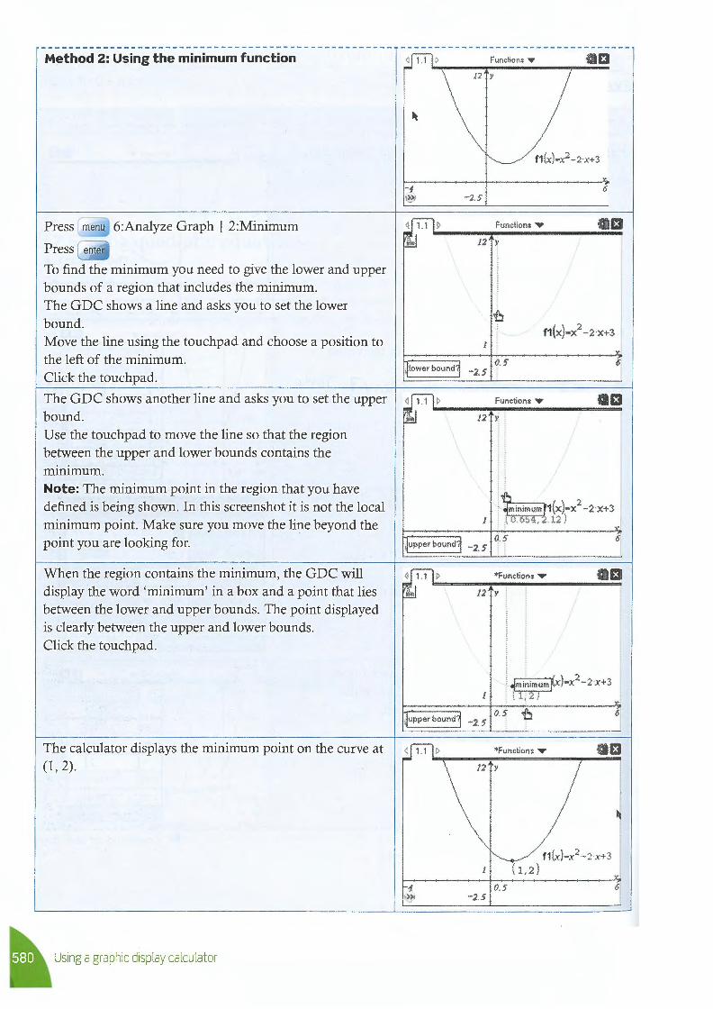
Method 2: Using the minimum function

Press

Press

6:Analyze Graph I 2:Minimum

To find the minimum you need to give the lower and upper bounds of a region that includes the minimum. The GDC shows a line and asks you to set the lower bound. Move the line using the touchpad and choose a position to the left of the minimum. Click the touchpad.

The GDC shows another line and asks you to set the upper bound. Use the touch pad to move the line so that the region between the upper and lower bounds contains the m1mmum. Note: The minimum point in the region that you have defined is being shown. In this screenshot it is not the local minimum point. Make sure you move the line beyond the point you are looking for.

When the region contains the minimum, the GDC will display the word 'minimum' in a box and a point that lies between the lower and upper bounds. The point displayed is clearly between the upper and lower bounds. Click the touchpad.

The calculator displays the minimum point on the curve at (1 , 2) .


Functions • £1 12 y

,.. 6

-2. 5

Functions .,.. £1 12 Y

f1 (x)=x2 -2 x+3

t::::::=:::::=::::::--+-0-5---------; ~lower bound] _2. 5 ·

Functions T £1

; ~tin~s~t J1 (x)=x2

- 2 ·x+ 3 I · ;l . , .12) ______________ ___,.,..

-2. s °:·f 6

*Functions T £1 12 Y )

: ~min27m~x)-x2-2-x+3

\ 1, ______________ __,.,..

Jupper bound] _2. 5 O. ~ tJ 6

-1 )

*Functions .,.. £1 12 y

0. 5 -2. 5

f1 (x)=x2-2-x+3 ( 1, 2)

Example 9

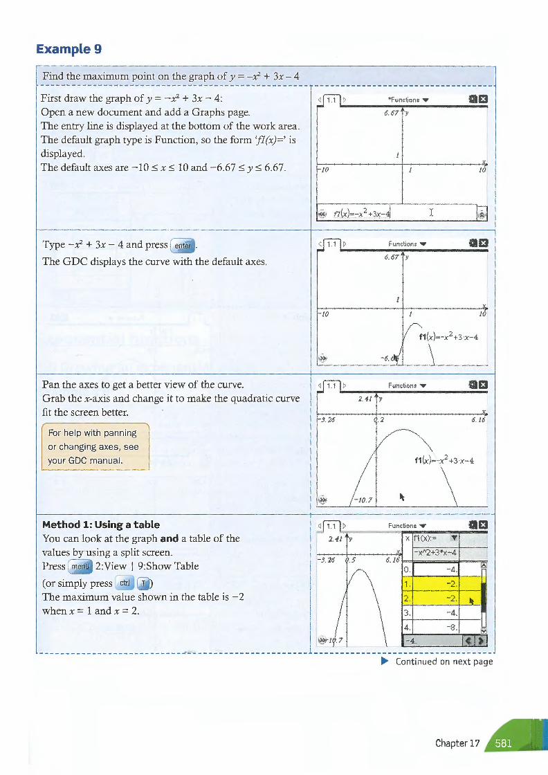
Find the maximum point on the graph of y = - x2 + 3x - 4

First draw the graph of y = - x2 + 3x - 4: Open a new document and add a Graphs page. The entry line is displayed at the bottom of the work area. The default graph type is Function, so the form 'fl (x)=' is displayed. The default axes are -10 :::; x:::; 10 and -6.67:::; y:::; 6.67.

Type -x2 + 3x - 4 and press enter .

The GDC displays the curve with the default axes.

Pan the axes to get a better view of the curve. Grab the x-axis and change it to make the quadratic curve fit the screen better.

For help with panning

or changing axes, see

your GDC manual.

Method 1: Using a table You can look at the graph and a table of the values by using a split screen. Press menu 2:View I 9:Show Table

( or simply press ctr!

The maximum value shown in the table is -2 when x = l and x = 2.

- JO

-JO

-3.26

lf 7

..

*Functions ,..

6.67 y

X

10

I

Functions ..., £1 6.67 y

X

10

f1(x)=-x2+3 ·x-4

Functions ..., £1

X

6.16

f1(x)=-x2+3 ·x-4

Functions ..., «1 £1 X f1 (X):= T

X - xA2+ 3*x- 4 6.16

0. -4.

1. - 2.

2. -2.

3. -4.

4. -8, IS2l

-4. C > • Continued on next page

Chapter 17

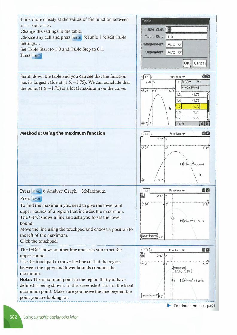
Look more closely at the values of the function between x = I and x = 2. Change the settings in the table. Choose any cell and press menu 5 :Table I 5 :Edit Table Settings ... Set Table Start to 1.0 and Table Step to 0.1.

Scroll down the table and you can see that the function has its largest value at (1.5 , -1. 75). We can conclude that the point ( 1. 5, - 1. 7 5) is a local maximum on the curve.

Method 2: Using the maximum function

To find the maximum you need to give the lower and upper bounds of a region that includes the maximum. The GDC shows a line and asks you to set the lower bound. Move the line using the touchpad and choose a position to the left of the maximum. Click the touchpad.

The GDC shows another line and asks you to set the upper bound. Use the touch pad to move the line so that the region between the upper and lower bounds contains the maximum. Note: The maximum point in the region that you have defined is being shown. In this screenshot it is not the local maximum point. Make sure you move the line beyond the point you are looking for.


Table

Table Start: 11 ~=======~ Table Step: 11 .0

:=:====;---------' Independent: I Auto vi

Dependent: I Auto v i

Functions ,.. £1 X f1 (x): = T

- x"2+ 3*x-4 -J.26 .5 6.16

1.3 -1 .79 l1Sl

1.4 - 1.76

I ~ 1.5 -1.75

1.6 - 1.76

1.7 -1.79 Ei1l -1.75 C >

Functions ,.. GIEi 2.41 y

" -J.26 0.2 6. 16

f1 (x)=-x2+3 ·x-4

-JO. 7

Functions ,.. CIEi 2.41 y

" -J.26 . 2 6.16

f1 (x)=-x2+3x-4

jtower boundJo. 7

Functions ,.. CIEi

" -J.26 0.2 6. 16 1 : maximum I . 1.1 , -1.87)

Jupper bound~. 7


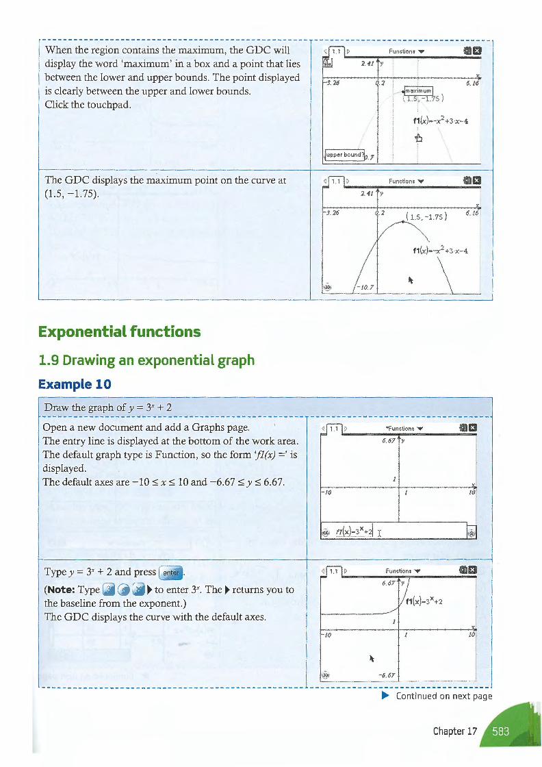
When the region contains the maximum, the GDC will display the word 'maximum' in a box and a point that lies between the lower and upper bounds. The point displayed is clearly between the upper and lower bounds. Click the touchpad.

The GDC displays the maximum point on the curve at (1.5, -1. 75).

Exponential functions

1.9 Drawing an exponential graph

Example 10

Draw the graph of y = 3x + 2

Open a new document and add a Graphs page. The entry line is displayed at the bottom of the work area. The default graph type is Function, so the form 'fl (x) =' is displayed. The default axes are -10 :s; x :s; 10 and -6.67 :s; y :s; 6.67.

Type y = 3x + 2 and press enter .

(Note: Type 3 " x • to enter 3". The • returns you to the baseline from the exponent.) The GDC displays the curve with the default axes.

Function•...,. 13 2.41 y

X'.

-J.26 0.2 6.16 maximum

l. r - 1. s l

f1(x)=-x2+3x-4

Jupper bound 1. 7

Functions ...,. 13 2. 41 y

X

-J.26 .2 ( 1.S , -1.7S) 6. 16

f1(x)=-x2+3·x-4

> -JO. 7

*Functions ...,. 13 6.67 y

-10

Functions ...,. 13

X'.

-10 lO

-6.67


Chapter 17




Grab the x-axis and change it to make the exponential curve fit the screen better.

For help with changing

axes, see your GDC

manual.

1.10 Finding a horizontal asymptote

Example 11

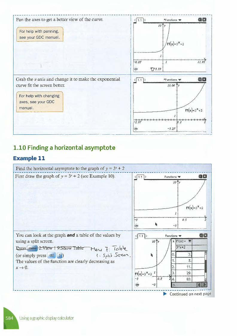
Find the horizontal asymptote to the graph of y = 3x + 2 ---------------------------------------------------First draw the graph of y = 3x + 2 (see Example 10).

You can look at the graph and a table of the values by using a split screen.

£J:es~~ z:vtew-J~~Tia1bte--~_, 1: (cJ,~ (or simply press ( , Sr\i~ 5q--eR,". The values of the function are clearly decreasing as x • 0.


-8.05

-2.97

i

- 3

'{]-3. 33

f1(x) -3X+2 J

-J 0.5

-J

*Functions ...,. £1

1/.95

*Functions -.

10.06 Y

0.2 2

-3. 27

Functions ...,. Gl£1 10 Y

0.5 2

-3

GEi X f1(x):= T

3.

1' 5.

2. 11.

3. 29.

2 4. 83.

3. C > ----------------------------------• Continued on next page

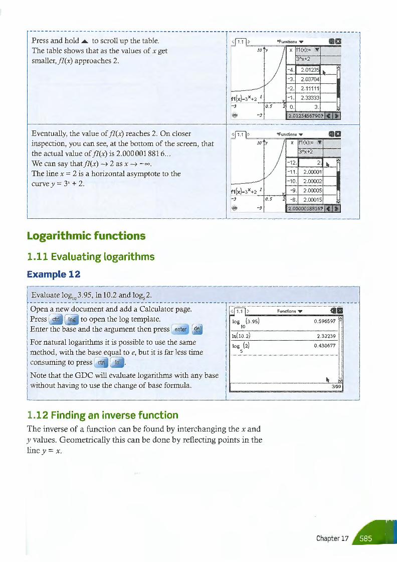
--------------------------------------------------------------- ----------------------------------Press and hold • to scroll up the table. The table shows that as the values of x get smaller,JJ(x) approaches 2.

Eventually, the value of fl(x) reaches 2. On closer inspection, you can see, at the bottom of the screen, that the actual value of fl(x) is 2.0000018816 ... We can say thatfl(x) • 2 as x • - 00 •

The line x = 2 is a horizontal asymptote to the curve y = 3x + 2.

Logarithmic functions

1.11 Evaluating logarithms

Example 12

Evaluate log10

3.95, In 10.2 and log52.

Open a new document and add a Calculator page. log to open the log template.

For natural logarithms it is possible to use the same method, with the base equal to e, but it is far less time consuming to press ctrt

Note that the GDC will evaluate logarithms with any base without having to use the change of base formula.

1.12 Finding an inverse function

f1(x)•3X+2 J -, -,

10

-,

jii1> log (3.95)

10

ln(l0 .2)

log (2) 5

The inverse of a function can be found by interchanging the x and y values. Geometrically this can be done by reflecting points in the line y = x.

0. 5

X f1(x):= T

3Ax+2

-4. 2.0123

-3. 2.03704

-2. 2.11 111

-1. 2.33333

3.

• £1

2.0123456790J C >

"Functions ..- • £1

-12. 2. 1/Sl

-11 . 2.CXX:01

-~ -10. 2.CXX:02

-9 . 2.CXX:05

2 -8. 2.0C015 l'Sil 2.0000018816, C >

Functions • ~£1 0.596597 i;;;i

2.32239

0.430677

~ IS1l 3199

Chapter 17

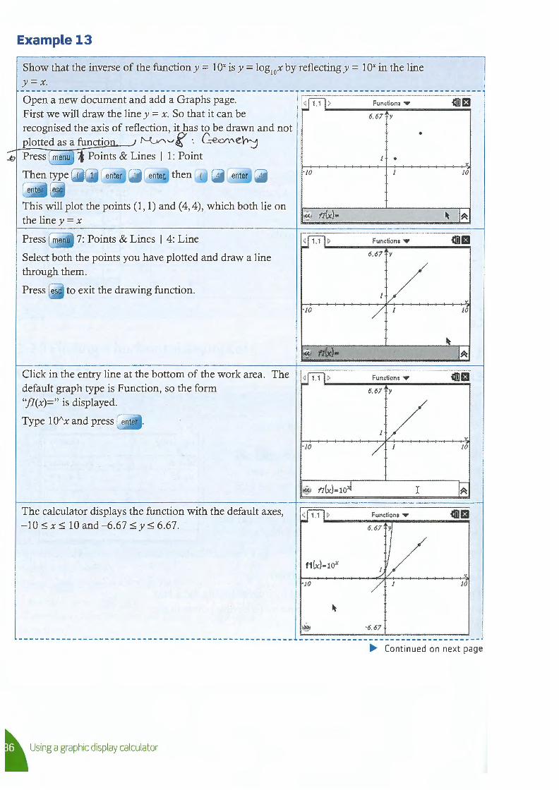
Example 13

Show that the inverse of the function y = lox is y = log10

x by reflecting y = lox in the line y=x.

Open a new document and add a Graphs page. First we will draw the line y = x. So that it can be recognised the axis of reflection, it has to be drawn and not plotted as a functio ~._,f ·. C,--e.c,,,."e~

1 Points & Lines I 1: Point

Then type (

This will plot the points (1, 1) and (4, 4), which both lie on the line y = x

Press menu 7: Points & Lines I 4: Line

Select both the points you have plotted and draw a line through them.

Press esc to exit the drawing function.

Click in the entry line at the bottom of the work area. The default graph type is Function, so the form ''j](x)=" is displayed.

The calculator displays the function with the default axes, - 10 ~ x ~ IO and-6.67 ~ y ~ 6.67.

J,17 :,

-10

I~ n(x)-

-10

-10

-JO

Functions .,..

6.67 y

•

I· • l

Functions•

Functions .,..

6.67 Y

I

Functions •

-6.67

~-• X:

10

'-: 1~

X:

JO

10

X:

JO



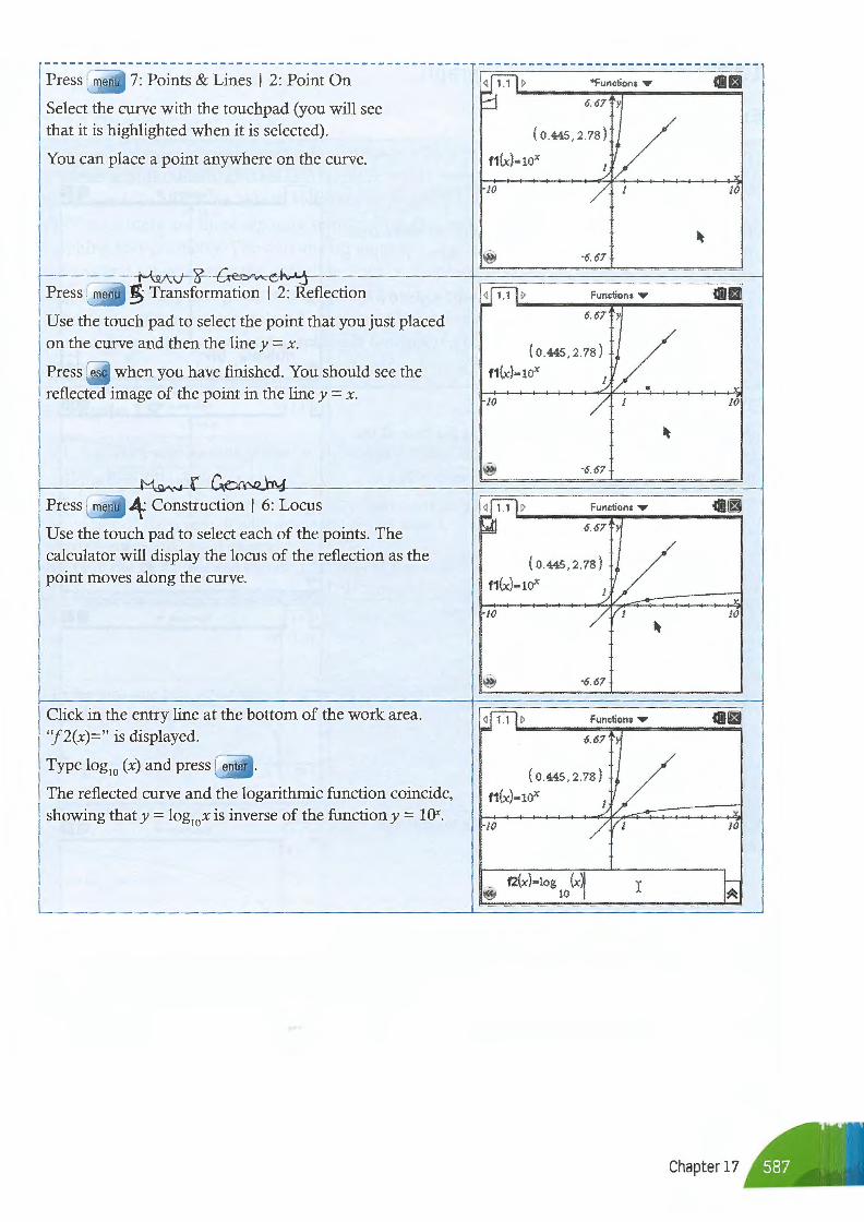
Press menu 7: Points & Lines I 2: Point On

Select the curve with the touchpad (you will see that it is highlighted when it is selected).

You can place a point anywhere on the curve.

Press menu ~ Transformation I 2: Reflection

Use the touch pad to select the point that you just placed on the curve and then the line y = x.

Press esc when you have finished. You should see the reflected image of the point in the line y = x.

Press menu 4 Construction I 6: Locus

Use the touch pad to select each of the points. The calculator will display the locus of the reflection as the point moves along the curve.

Click in the entry line at the bottom of the work area. ''f2(x)=" is displayed.

The reflected curve and the logarithmic function coincide, showing that y = log

10x is inverse of the function y = I ox.

"'Functions •

6.67 y

( 0 .445, 2.78)

f1 (x)-1ox

· JO

·6.67

Functions •

6.67 y

(0.445,2.78)

f1 (x)=10x

·JO

·6.67

•

Functions •

6.67 y

(0 .445,2 .78)

f1 (x)= l 0x

·JO

·6.67

Functions•

( 0.445, 2.78)

f1 (x)- 1oX

· JO

f2(x)=log (x~ 10 ,, I

:c 10

10

:c 10

10

Chapter 17

1.13 Drawing a logarithmic graph

Example 14

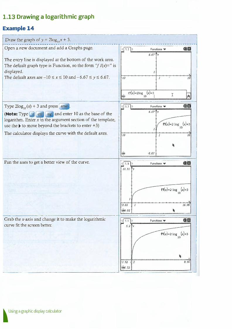
Draw the graph of y = 2log10x + 3.

Open a new document and add a Graphs page.

The entry line is displayed at the bottom of the work area. The default graph type is Function, so the form "J l(x)=" is displayed. The default axes are - 10 ~ x ~ 10 and-6.67 ~ y ~ 6.67.

Type 2log10

(x) + 3 and press enter .

(Note: Type 2 ctrl log and enter 10 as the base of the logarithm. Enter x in the argument section of the template, use the • to move beyond the brackets to enter +3)

The calculator displays the curve with the default axes.


Grab the x-axis and change it to make the logarithmic curve fit the screen better.


jul> Functions ,.. cmm 6.67 ~y

1 X

·/0 1 10

I~ fl(x)=2log (x)+3

10 I I ~

· JO

10. 31 Y

·3.02

Functions ,.. Clil£1 6.67 y

·6.67

f1(x)=2· log (x)+3 10

X

10

Functions ,..

f1(x)=2·log (x)+3 10

X

16. 98

Functions ,..

8.56

Trigonometric functions

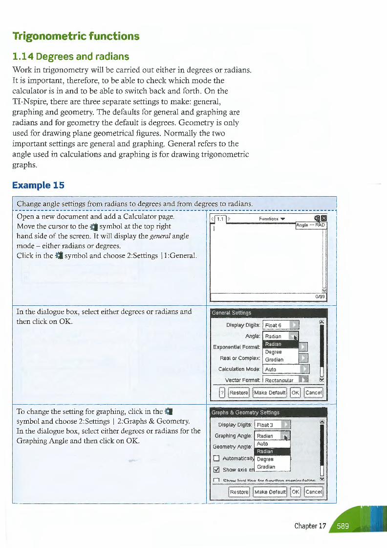
1.14 Degrees and radians Work in trigonometry will be carried out either in degrees or radians. It is important, therefore, to be able to check which mode the calculator is in and to be able to switch back and forth. On the TI-Nspire, there are three separate settings to make: general, graphing and geometry. The defaults for general and graphing are radians and for geometry the default is degrees. Geometry is only used for drawing plane geometrical figures. Normally the two important settings are general and graphing. General refers to the angle used in calculations and graphing is for drawing trigonometric graphs.

Example 15

Change angle settings from radians to degrees and from degrees to radians. --------------------------------------------------- ----------------------------------Open a new document and add a Calculator page. ~ > Functions .... ID Move the cursor to the {{I symbol at the top right

1 1Angle -- RAD

hand side of the screen. It will display the general angle mode - either radians or degrees. Click in the {€1 symbol and choose 2:Settings 11 :General.

In the dialogue box, select either degrees or radians and then click on OK.

To change the setting for graphing, click in the a symbol and choose 2:Settings I 2:Graphs & Geometry. In the dialogue box, select either degrees or radians for the Graphing Angle and then click on OK.

General Settings

Display Digits: I Float 6

Angle:

Exponential Format:

Real or Complex: Gradian \.-----~=.

Calculation Mode: Auto :=======:;'

Vector Format: I Rectanaular

0199

t} j Restore j j Make Default! lo~ j cancel l

Graphs & Geometry Settings


Graphing Angle: 1----Geometry Angle:

0 Automatical

G?l Show axis e,~---~

n ~hnw tnnl t ine fnr f11nr-tinl"'I m-oniru,l~tlnn ~

Chapter 17

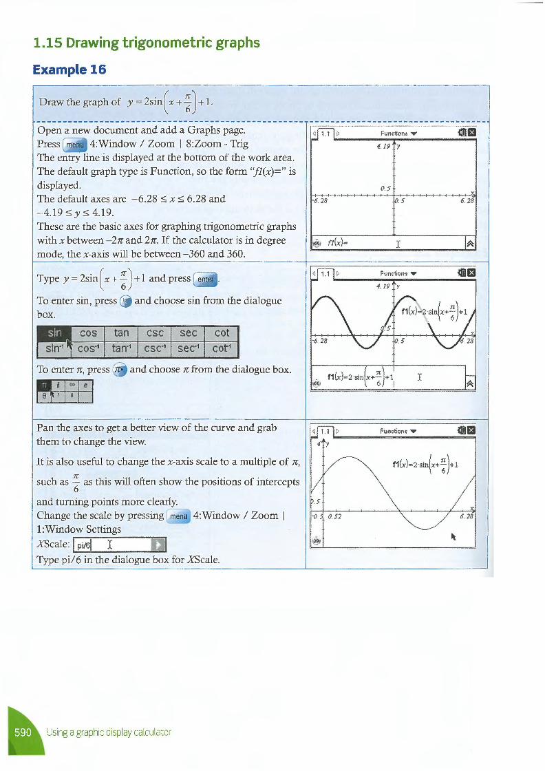
1.15 Drawing trigonometric graphs

Example 16

Draw the graph of y = 2sin ( x + ; ) + 1.

Open a new document and add a Graphs page. Press menu 4:Window / Zoom. I 8:Zoom. - Trig The entry line is displayed at the bottom. of the work area. The default graph type is Function, so the form. "fl(x)=" is displayed. The default axes are -6.28 ::; x :s; 6.28 and -4.19 :s;y :s; 4.19. These are the basic axes for graphing trigonometric graphs with x between -2n and 2n. If the calculator is in degree mode, the x-axis will be between -360 and 360.

Type y = 2sin ( x + ; ) + I and press enter .

To enter sin, press ~g and choose sin from. the dialogue box.

tan csc sec cot

tan-1 csc·1 sec1 cot1

To enter n, press n• and choose n from. the dialogue box.

Pan the axes to get a better view of the curve and grab them. to change the view.

It is also useful to change the x-axis scale to a multiple of n,

such as 1r as this will often show the positions of intercepts 6

and turning points more clearly. Change the scale by pressing menu 4: Window / Zoom. I 1: Window Settings

.XScale: I pil6j I Type pi/ 6 in the dialogue box for .XScale.


jul> Functions ...,. «ma 4. 19 I Y

0. 5 --,:

·6. 28 0. 5 6. 28

I~ fl(x)= I 1~

- f1(x)=2·sin(x+~)+ 11

I < 6 I

Functions ...,. l1iJ £f

f1 (x)=2·sin(x+J )+ 1

. 5

·O. Si 0. 52 6. 28

;

-----------More complicated functions

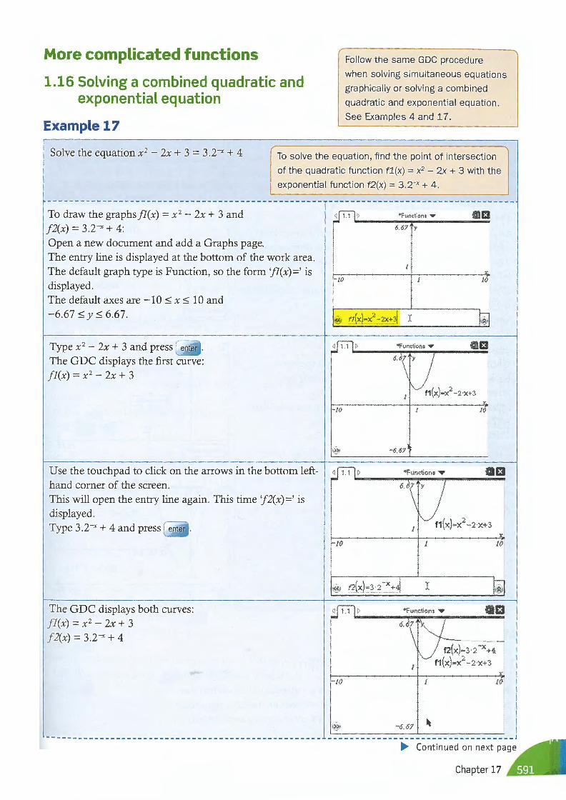
1.16 Solving a combined quadratic and exponential equation

Example 17

Follow the same GDC procedure

when solving simultaneous equations

graphically or solving a combined

quadratic and exponential equation.

See Examples 4 and 17.

Solve the equation x 2 - 2x + 3 = 3.2-x + 4 To solve the equation, find the point of intersection

of the quadratic function f1(x) = x2 - 2x + 3 with the

exponential function f2(x) = 3.2-x + 4.___ J To draw the graphs j].(x) = x 2

- 2x + 3 and f2(x) = 3,2-x + 4:

Open a new document and add a Graphs page. The entry line is displayed at the bottom of the work area. The default graph type is Function, so the form 'j].(x)=' is displayed. The default axes are - 10 ~ x ~ 10 and -6.67 ~ y ~ 6.67.

Type x 2 - 2x + 3 and press enter .

The GDC displays the first curve: fl(x) = x 2 - 2x + 3

Use the touchpad to click on the arrows in the bottom lefthand corner of the screen. This will open the entry line again. This time 'f 2(x) =' is displayed. Type 3 .2-x + 4 and press enter .

The GDC displays both curves: fl (x) = x 2 - 2x + 3 J2(x) = 3,2-x + 4

---------------------------------------------------

< 1.1 > *Functions ...,. 13 ~------r-------6.67 y

-10 10

<< n(x)-x2

-2x+31 X

*Functions ..,. 13

f1(x)-x2 - 2 x+3

-10 10

- 6.67

*Functions • £1

f1(x)=x2 - 2-x+3

- JO J JO

I

*Functions ...,.

X

- JO 10

> - 6. 67

• Chapter 17

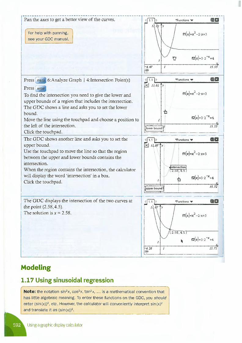
Pan the axes to get a better view of the curves.



Press 6:Analyze Graph I 4:Intersection Point(s)

Press

To find the intersection you need to give the lower and upper bounds of a region that includes the intersection. The GDC shows a line and asks you to set the lower bound. Move the line using the touchpad and choose a position to the left of the intersection. Click the touchpad.

The GDC shows another line and asks you to set the upper bound. Use the touch pad to move the line so that the region between the upper and lower bounds contains the intersection. When the region contains the intersection, the calculator will display the word 'intersection' in a box. Click the touchpad.

The GDC displays the intersection of the two curves at the point (2.58, 4.5). The solution is x = 2.58.

Modeling

1.17 Using sinusoidal regression

-1.28 )

Note: the notation sin2 x, cos2x, tan2x, .. . is a mathematical convention that

has little algebraic meaning. To enter these functions on the GDC, you should

enter (s in (x))2, etc . However, the calculator will conveniently interpret sin (x)2

and translate it as (sin(x))2.


*Functions .,.. f3

f1(x)=x2-2 ·x+3

X

15.53

*Functions "' f3

f1(x)=x2 - 2 x+3

f2(x)=3·2-x+4

*Functions "'

f i f1(x)-x2 -2 ·x+3

I

X

15.53

Gf3

f2(x)=3 ·2 -x+4

15.72

f3

f1(x)=x2

-2 x+3

15.72

/

Example 18

It is known that the following data can be modeled using a sine curve.

I ; I 6°9 I 91

4172916

3719

4218

5316

6

51879 I

Use sine regression to find a function to model this data. ---------------------------------------------------Open a new document and add a Lists & Spreadsheet page. Type 'x' in the first cell and 'y' in the cell to its right. Type the numbers from the x-list in the first column and those from they-list in the second. Use the ..., • • • keys to navigate around the spreadsheet.

< 11-11 > •• x

~

iC

3

~

~

0

1

2

3

4

Functions •

!!ly g !I

6.9

9.4

7.9

6.7

9.2 ...

iffll3 !iS

-

-

~

MB'-V

4: Skt~r \ :Skl-

c""'' \tck v c: r; ,, Of\ r. I -----------------------+-r-- _- _- _- _- _- _- _- _- _- _- _- _---:_---:_- _- _- _- _- _- _- _- _- _- _- _- _- _---j /k

Al lo ·• 1 

): Dciu

;,(tt,ti ct

Press ~ On and add a new graphs page to your document. Functions • ili!l3 j '

,. &wt ~(,V'

·vv1ct0liz •~1 (o r

.~f,ct,.I

<M''~

Press 3:Graph Type I 6:Scatter Plot

Press

The entry line is displayed at the bottom of the work area. Scatter plot type is displayed. Enter the names of the lists, x and y, into the scatter plot function

Adjust your window settings to show your data and the xand y-axes. You now have a scatter plot of x against y.

~ Press ctrl • to return to the Lists & Spreadsheet page. Its Select an empty cell and press menu 4:Statistics I Stat

Calculations I C:Sinusoidal Regression ... ies!' · Tress enter

1 ~rom the drop down menus choose 'x' for X List and 'y' for •~4SOIV .

I List. You should press tab to move between the fields.

'II Press enter

-10

- s1 <1

12

_,._ -2

y

{x .... X y.... ~

(x,y) •

•

J

6.67 y

)(

/0

Functions •

• •

• •

~

8

Sinusoidal Regression

X list x :=::======: Y List y !=:======~

Save RegEqn to: fl :=::======: Iterations: 8 !:======~

Period: (optional)

Cateqorv list I ,~ • Continued on next page

Chapter 17

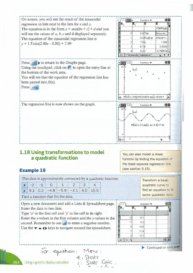
On screen, you will see the result of the sinusoidal regression in lists next to the lists for x and y. The equation is in the form y = asin(bx + c) + d and you will see the values of a, b, c and d displayed separately. The equation of the sinusoidal regression line is y = 1.51sin(2.00x- 0.80) + 7.99

Press ctrl • to return to the Graphs page. Using the touch pad, click on > > to open the entry line at the bottom of the work area. You will see that the equation of the regression line has been pasted into fl(x).

The regression line is now shown on the graph.

1.18 Using transformations to model a quadratic function

Example 19

This data is approximately connected by a quadratic function,

I ; I ~-~ I ~-~ I -~-8 I -:.9 1 -:.1 143

0 I 1:.0 I Find a function that fits the data.

1 0 6.9 Title Sinusoid ...

9.4 RegEqn a"'sin(b*x ...

2 7 .9 a 1. 506

3 6.7 b 2.0029

4 9.2 C ·0.799874 ~

C > --- - -- ~- -- -

Function ; T ili]Ef 12 y

(x,y) . . . .

f1(x) • 1.51 ·sin(2 x+ -0.8)+7 99

-2 8

You can also model a linear

function by finding the equation of

the least squares regression line

(see section 5.15) .

Transform a basic

quadratic curve to

find an equation to fit

some quadratic data.

--------------------------------------------------- ------------------------------- ---Open a new document and add a Lists & Spreadsheet page. Enter the data in two lists: Type 'x' in the first cell and 'y' in the cell to its right. Enter the x-values in the first column and they-values in the 1

second. Remember to use (-) to enter a negative number. Use the ..., ..., • • keys to navigate around the spreadsheet.

Al

- 2

-1

0

2

-2 It

£1 "'

9.1

0.2

-4.8

-S.9

-3.1

C > ---------------------- ---- --------

k)r- 9"..,t Gl~0- ·.

4 Using a graphic display calculator I ;

M -'cf'.. 0

S'ro}-f Sratr Co.le """ . _, ()- ~


Add a Graphs page to your document. Press menu 3:Graph Type I 4:Scatter Plot

The entry line is displayed at the bottom of the work area. Scatter plot type is displayed. Enter the names of the lists, x and y, into the scatter plot function. Use the tab key to move from x toy.

Press

Press A:Zoom-Fit from the Window/Zoom menu This is a quick way to choose an appropriate scale to show all the points. You should recognize that the points are in the shape of a quadratic function.

The next step is to enter a basic quadratic function, y = x2, and manipulate it to fit the points. Press menu 3:Graph Type I !:Function

This changes the graph type from scatter plot to function. Type x2 in as functionfl(x). It is clear that the curve does not fit any of the points, but it is the right general shape to do so.

Use the touch pad to move the cursor so it approaches the curve. You will see one of two icons. The first will allow you to drag the quadratic function around the screen by its vertex.

The second allows you to stretch the function either vertically or horizontally.

Use + to position the vertex where you think it ought to be according to the data points.

------ ------------------------------------------

----------------*Quadratic • CIEi

6.67 y

1

- JO 1 ~ 10

{;;; 1.2 > Quad ratic •

17 y •

. •

-2. s 4.S •

- 8 • (x,y)

1.2 > Quadratic ,.., {§)£1 17 y •

• f1(x)=x 2

• ~

- 2. s 4.S •

~ - 8 • (x,y)

t graph f1· Dns4• : f _, or

"" graph f1 ~¾

' 1.2 > *Quadratic ""' {§)£1 17 y •

f1(x)=(x- 0.66)2- 6

•

4.S

• (x,y)


Chapter 17

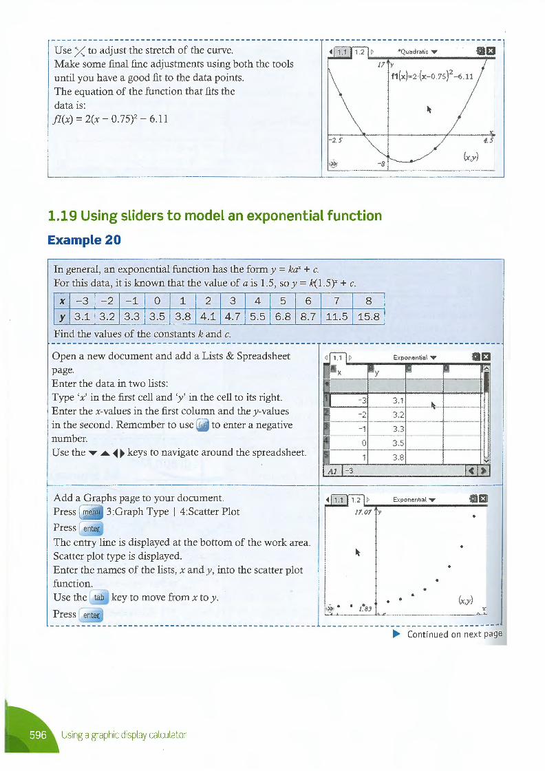
Use X to adjust the stretch of the curve. Make some final fine adjustments using both the tools until you have a good fit to the data points.

17 y

The equation of the function that fits the data is: fl(x) = 2(x - 0. 75)2 - 6.11

-2.s

1. 19 Using sliders to model an exponential function

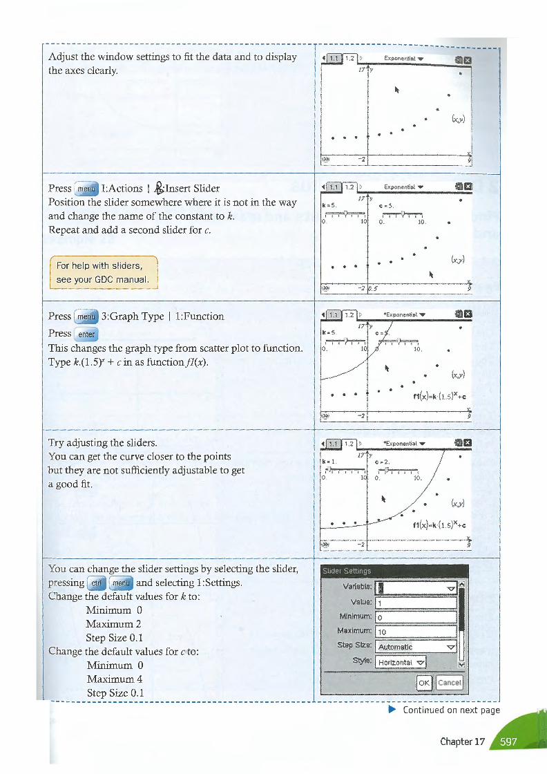
Example 20

In general, an exponential function has the form y = kax + c. For this data, it is known that the value of a is 1.5, soy= k(l.5Y + c.

X -3 -2 -1 0 1 2 3 4 5 y 3.1 3.2 3.3 3.5 3.8 4.1 4.7 5.5 6.8

Find the values of the constants k and c.

Open a new document and add a Lists & Spreadsheet page. Enter the data in two lists: Type 'x' in the first cell and 'y' in the cell to its right. Enter the x-values in the first column and they-values in the second. Remember to use (-) to enter a negative number.

6 8.7

Use the ...,. • • • keys to navigate around the spreadsheet.

7

11.5

Al - 3

8 15.8

f1(x)=2·(x-0. 7S)2 - 6 . ll

4.5

(x,y)

( >

Add a Graphs page to your document. Press menu 3:Graph Type I 4:Scatter Plot

1.2 > Exponential"' 13

The entry line is displayed at the bottom of the work area. Scatter plot type is displayed. Enter the names of the lists, x and y, into the scatter plot function. Use the tab key to move from x toy.

17.07 y

• •

•

•

• (x,y)

X:

--------------------------------------------------- ----------------------------------• Continued on next page


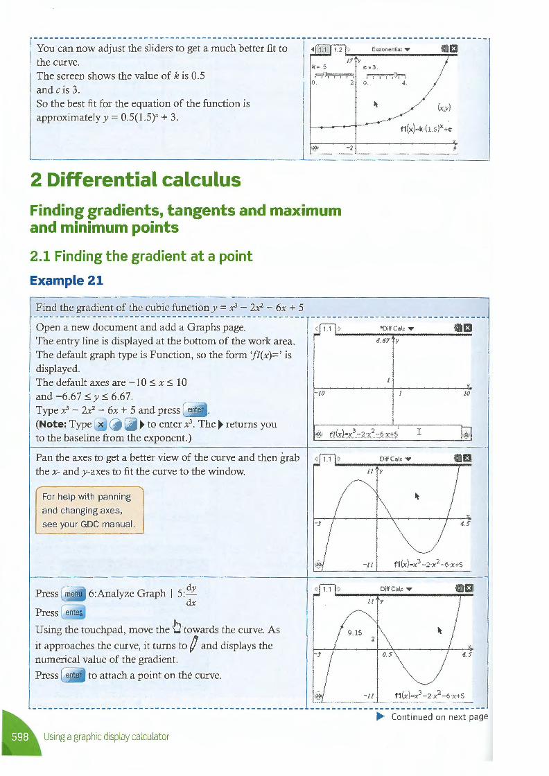
Adjust the window settings to fit the data and to display the axes clearly.

Press menu !:Actions I iinsert Slider Position the slider somewhere where it is not in the way and change the name of the constant to k. Repeat and add a second slider for c.

For help with sliders,


Press menu 3:Graph Type I 1:Function

This changes the graph type from scatter plot to function. Type k.(l .5Y + c in as functionfl(x).

Try adjusting the sliders. You can get the curve closer to the points but they are not sufficiently adjustable to get a good fit.

You can change the slider settings by selecting the slider, pressing ctrl menu and selecting 1 :Settings. Change the default values fork to:

Minimum 0 Maximum2 Step Size 0.1

Change the default values for c to: Minimum 0 Maximum4 Step Size 0.1

----------------~ 1 . 2 I > Exponential • •a

17 y . ~ •

. . (x,y) . • • • • . .

" ~ -2 9

Exponential • £1 17 y .

k •S . e =5 .

~ t"F.~ 0. 10 0 . 10 . .

. . • (x,y) . . . . •

~

.5 9

*Exponential • £1 17 y .

k •S .

. ,~ 0. lO. .

~ • • (x,y)

• . . . f1 (x);k (1.s)x+c . . .

> -2 9

1.2 i *Exponential • £1 l7 y •

k • l. e •2 . rJ,.=-.-,,""", :=f>=,=,=,=,=,

0 . 1 . 0 . 10 . •

(x,y)

. . . > 9

Slider ·:c.ett1r11J,-

Variable:! I v-1~

Value: 11 Minimum: lo

Maximum: I 1 o Step Size: I Automatic v-1

Style: I Horizontal v-1 I [OK] [ Cancel]

------ -- ---- ----- --- ---------- ---- --- -------- ------ ------------------ ----------------• Continued on next page

Chapter 17

You can now adjust the sliders to get a much better fit to the curve. The screen shows the value of k is 0.5 and c is 3. So the best fit for the equation of the function is approximately y = 0.5(1.5Y + 3.

2 Differential calculus

Exponential ,..

17 y k •.5 c -3 .

Ff~~~ 0. 2 . 0 . 4 .

Cl

(x,y)

X

9

Finding gradients, tangents and maximum and minimum points

2.1 Finding the gradient at a point

Example 21

Find the gradient of the cubic function y = .x3 - 2x2 - 6x + 5

Open a new document and add a Graphs page. The entry line is displayed at the bottom of the work area. The default graph type is Function, so the form 'fl(x)=' is displayed. The default axes are -10 ~ x ~ 10 and -6.67 ~ y ~ 6.67. Type .x3 - 2x2 - 6x + 5 and press enter .

(Note: Type x I\ 3 • to enter .x3. The • returns you to the baseline from the exponent.)

Pan the axes to get a better view of the curve and then grab the x- and y-axes to fit the curve to the window.

For help with panning

and changing axes,


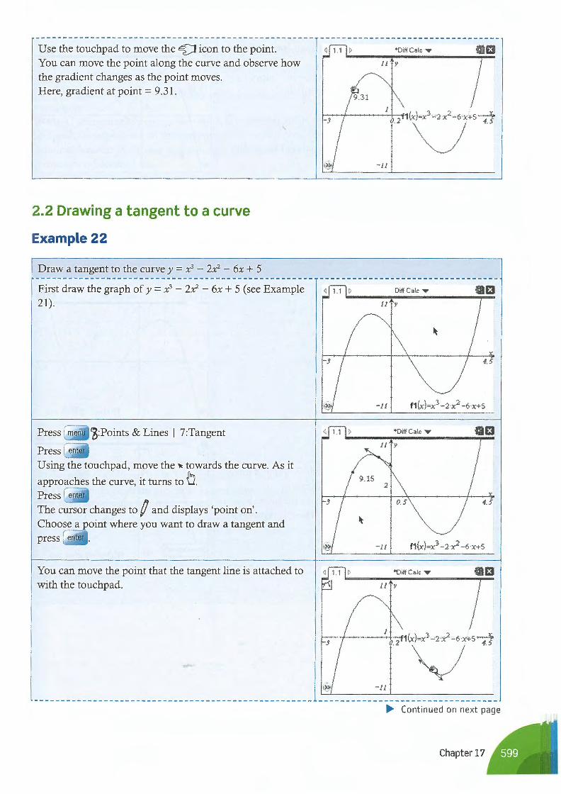
Press menu 6:Analyze Graph I 5: dy dx

Press enter

Using the touch pad, move the -!J towards the curve. As

it approaches the curve, it turns to / and displays the numerical value of the gradient.

Press enter to attach a point on the curve.


-lO

9.15

*Diff Cale ..,. 13 6.67 y

X

10

X

11 y

- 11

13 1 l y

2

4.5

-11 f1 (x)=x3 -2-x2-6-x+S


Use the touch pad to move the c'[J icon to the point. You can move the point along the curve and observe how the gradient changes as the point moves. Here, gradient at point = 9. 31.

2.2 Drawing a tangent to a curve

Example 22

Draw a tangent to the curve y = x3 - 2x2 - 6x + 5

First draw the graph of y = x3 - 2x2 - 6x + 5 (see Example 21).

Press menu 'g:Points & Lines I 7:Tangent

Press enter

Using the touch pad, move the ~ towards the curve. As it

approaches the curve, it turns to b. Press enter

The cursor changes to f and displays 'point on'. Choose a point where you want to draw a tangent and

You can move the point that the tangent line is attached to with the touchpad.

*OiffCalc • £1 11 )'

-11

£1 11 )'

- 3

-11 f1(x)=x3- 2x2- 6x+S

*DiffCalc • £1

0.5

-11 f1(x)=x3- 2·x2- 6-x+S

*Oiff Calc • £1 11 )'

--------1+++-41(x)=x3

- 2 x2

- 6 ·x+S -4 -, ., V ,., -11


Chapter 17

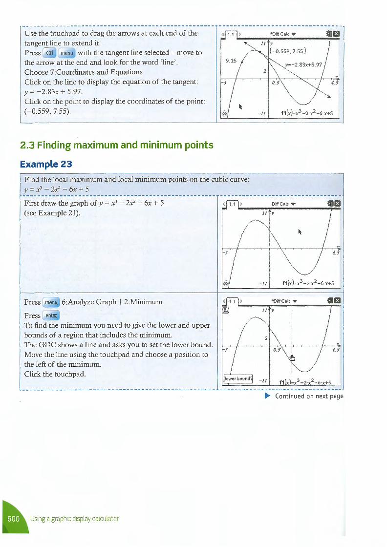
Use the touch pad to drag the arrows at each end of the £1 tangent line to extend it. Press ctrl menu with the tangent line selected - move to the arrow at the end and look for the word 'line'. Choose 7:Coordinates and Equations Click on the line to display the equation of the tangent: y = -2.83x + 5.97. Click on the point to display the coordinates of the point: (-0.559, 7.55).

2.3 Finding maximum and minimum points

Example 23

-J

Find the local maximum and local minimum points on the cubic curve: y = x3 - 2x2 - 6x + 5

First draw the graph of y = x3 - 2x2 - 6x + 5 (see Example 21).

Press enter

To find the minimum you need to give the lower and upper bounds of a region that includes the minimum. The GDC shows a line and asks you to set the lower bound. Move the line using the touchpad and choose a position to the left of the minimum.

-J

-11 f1 (x)=x3- 2·x2- 6·x+S

DiffCalc..,.

11 y

-11 f1(x)=x3-2 ·x2- 6·x+S

*Diff Calc..,. £1 11 y

2

Click the touchpad. 1 lower bound . _ 11



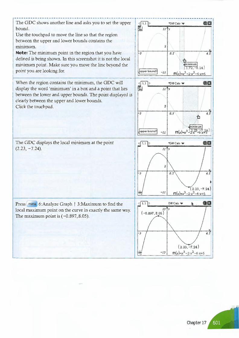
The GDC shows another line and asks you to set the upper bound. Use the touch pad to move the line so that the region between the upper and lower bounds contains the mm1mum. Note: The minimum point in the region that you have defined is being shown. In this screenshot it is not the local minimum point. Make sure you move the line beyond the point you are looking for.

When the region contains the minimum, the GDC will display the word 'minimum' in a box and a point that lies between the lower and upper bounds. The point displayed is clearly between the upper and lower bounds. Click the touchpad.

The GDC displays the local minimum at the point (2.23, - 7.24).

Press menu 6:Analyze Graph I 3:Maximum to find the local maximum point on the curve in exactly the same way. The maximum point is (-0.897, 8.05).

*DiffCatc • CIEi l1 y

2

1jupper bound] _ 11

Q.5 4.5

~ ~ .14 )

f1 x =x3-2·x2-6·x+S

*DiffCalc • CIEi 1/ y

2

Q.5

JupperboundJ -J/

*Diff Cale ...,. CIEi l1 y

0.5 4.5

-11

~

(2.23,-7 .24) f1 x =x3-2·x2-6·x+S

DiffCalc ..-

l!J y

( - 0.897, 8.05)

(2.23,-7 .24)

-l!J f1 (x)=x3-2·x2- 6·x+S

Chapter 17

Derivatives

2.4 Finding a numerical derivative Using the calculator it is possible to find the numerical value of any derivative for any value of x. The calculator will not, however, differentiate a function algebraically. This is equivalent to finding the gradient at a point graphically (see Section 2.1 example 21).

Example 24

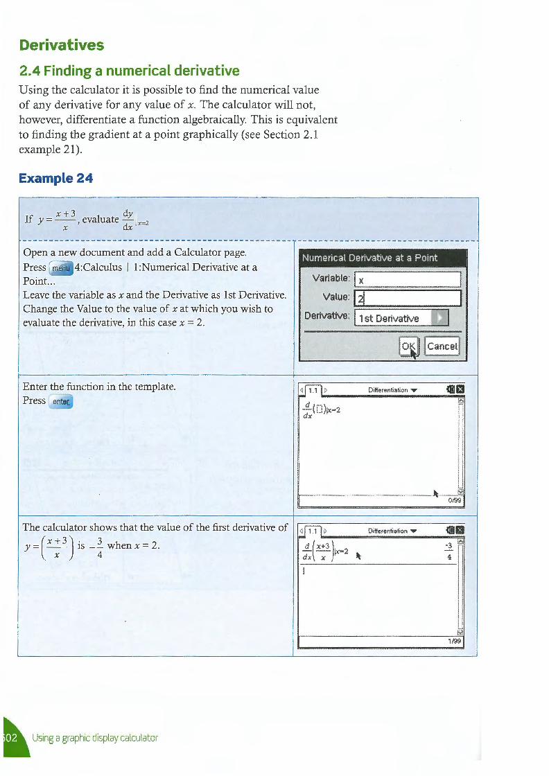
x +3 dy I If y = -x-, evaluate dx x=z

Open a new document and add a Calculator page.

Press menu 4:Calculus I 1 :Numerical Derivative at a Point ... Leave the variable as x and the Derivative as 1st Derivative. Change the Value to the value of x at which you wish to evaluate the derivative, in this case x = 2.

Enter the function in the template.

The calculator shows that the value of the first derivative of

(x+3) • 3 h _ 2 y = - x - 1s - 4 w en x - .


Numerical Deriv ative at a Point

Variable: I x ;;;;;;======~

Value:! 21 ~====::;:::=::;---'

Derivative: 11 st Derivative

Cancel

~ .. > ____ o_iff-er_en-tia-tio_n_ ..... ___ i1il_• m_ ~

~([~:)jx=2 dx

0199

~ > Differentiation T i1!1£1

~(x+3)ix=2 -3 ~ dx x ~ 4

I

f2l 1199

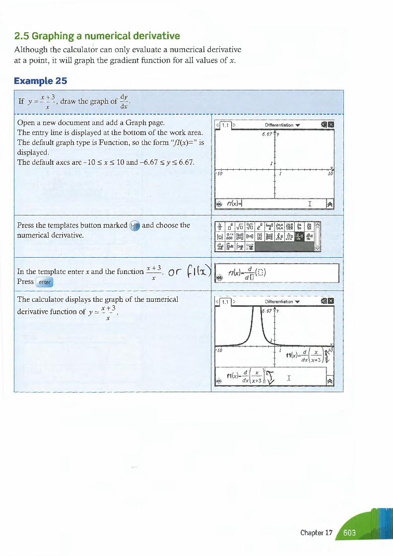
2.5 Graphing a numerical derivative Although the calculator can only evaluate a numerical derivative at a point, it will graph the gradient function for all values of x.

Example 25

x+3 dy If y = --, draw the graph of - .

X dx

Open a new document and add a Graph page. The entry line is displayed at the bottom of the work area. The default graph type is Function, so the form ''fl(x)=" is displayed. The default axes are -10 $ x $ 10 and - 6.67 $ y $ 6.67.

Press the templates button marked !•I ! and choose the numerical derivative.

In the template enter x and the function x + 3 . X

The calculator displays the graph of the numerical

d . . fu . f x+3 envat1ve nct10n o y = --. X

·JO

i•I g~• [g~J [oo] [g]

{jz J§do lllf ~'il

Differentiation 'Y

6.67 y

Differentiation 'Y

6.67 y

,c

10

:r

·JO I d ( x )~O f1(x)=- -dx x+3 \!,

. f1(x)=~(~)'1 X d x x+3 j V

Chapter 17

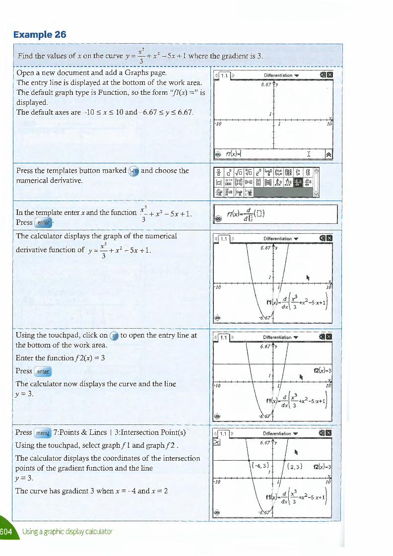
Example 26 3

Find the values of x on the curve y = ~ + x 2 -5x + 1 where the gradient is 3. 3

Open a new document and add a Graphs page. The entry line is displayed at the bottom of the work area. The default graph type is Function, so the form ''fl(x) =" is displayed. The default axes are -10 $ x $ 10 and-6.67 $ y $ 6.67.

Press the templates button marked [· II and choose the numerical derivative.

3

In the template enter x and the function ~ + x 2 - 5x + 1. 3

The calculator displays the graph of the numerical 3

derivative function of y = ~ + x 2 - 5x + 1.

3

Using the touch pad, click on > J to open the entry line at the bottom of the work area.

Enter the function/2(x) = 3

The calculator now displays the curve and the line y = 3.

Press menu 7:Points & Lines I 3:Intersection Point(s)

Using the touchpad, select graph/1 and graph/2.

The calculator displays the coordinates of the intersection points of the gradient function and the line y = 3.

The curve has gradient 3 when x = -4 and x = 2


~ >

-10

•~ fl(x)=I

-10

-JO

-JO

Differentiation ..., tm£f 6.67 y

1 X

1 10

I IA

Differentiation ...,

6.67 y

1 10

I d (x3 ) f1Cx}-- -+x2- S·x+l I dx 3

-6. 6-7


f2(x)=3 X

-6.6-7


f2(x)=3 X

1 10

r/ =!!__(x3

+x2-S ·x+ l) If, dx 3

-6.6-7

2.6 Using the second derivative The calculator can find first and second derivatives. The second derivative can be used to determine whether a point is a maximum or minimum point.

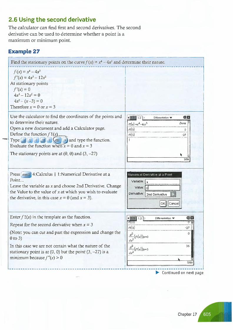
Example 27

Find the stationary points on the curvef(x) = .x4 -4x3 and determine their nature.

f(x) = .x4 - 4x3 f'(x) = 4x3 - 12.x2

At stationary points f'(x) = 0 4x3- 12.x2 = 0 4x2- (x-3) = 0

Therefore x = 0 or x = 3

Differentiation ..,.. Use the calculator to find the coordinates of the points and to determine their nature. fl(x) :-x4 - 4·x3 Done .sJ

Open a new document and add a Calculator page. Define the functionfl(x __ ,__ Type F 1 ( ) ctrl := and type the function. Evaluate the function when x = 0 and x = 3

The stationary points are at (0, 0) and (3, -27)

Press menu 4:Calculus I 1 :Numerical Derivative at a Point. .. Leave the variable as x and choose 2nd Derivative. Change the Value to the value of x at which you wish to evaluate the derivative, in this case x = 0 (and x = 3).

Enter f I (x) in the template as the function.

Repeat for the second derivative when x = 3

(Note: you can cut and past the expression and change the 0 to 3)

In this case we are not certain what the nature of the stationary point is at (0, 0) but the point (3, -27) is a minimum because f"(x) > 0

t1(0)

Numerical Derivative at a Point

Variable: Ix ;:::;::======

Value: !ol ~====:;::=;-.....

Derivative: I 2nd Derivative

.,.2]> Differentiation •

f1(3)

d2 -(t1(xl)1x=o d,_2

d2 - (t1(x))lx=3 d,_2

...

0

·27

3199

~a UfiS]

-27

0

36

f'i1l 5/99


Chapter 17

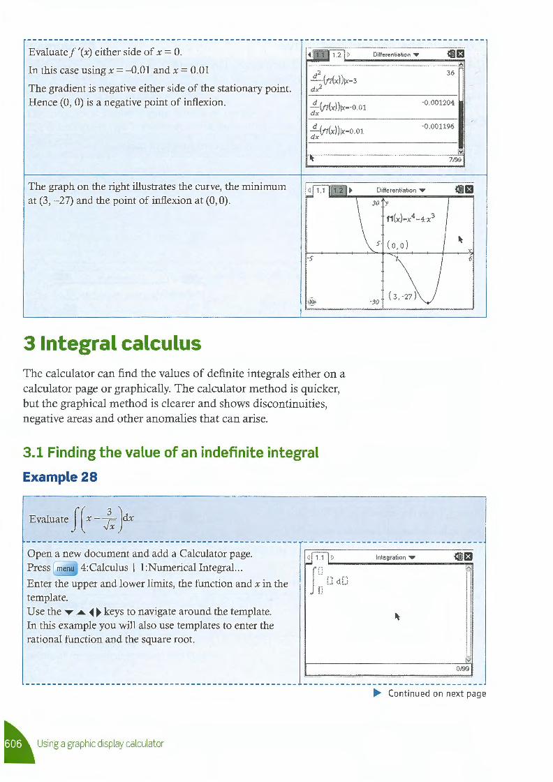
Evaluate/ '(x) either side of x = 0.

In this case using x = -0.01 and x = 0.01

The gradient is negative either side of the stationary point. Hence (0, 0) is a negative point of inflexion.

The graph on the right illustrates the curve, the minimum at (3, -27) and the point of inflexion at (0, 0).

3 Integral calculus

,!Bl.2j >

d2 - (r1(x) )!x=3 d/-

.E'...(r1(x))1x=·O .Ol dx

.E'...(r1(x) )ix=o o 1 dx

It

< 1.1

-5

The calculator can find the values of definite integrals either on a calculator page or graphically. The calculator method is quicker, but the graphical method is clearer and shows discontinuities, negative areas and other anomalies that can arise.

3.1 Finding the value of an indefinite integral

Example 28

Evaluate f ( x - }; )dx

Differentiation •

( 3, -27) ·30

~m [;,s

36

-0 .001204

-0 .001196

l'li 7199

X

6

Open a new document and add a Calculator page. Press menu 4:Calculus I !:Numerical Integral...

jul._> ____ i_nte_g_rat_io_n _,... ____ ilil_• m .....

I[] l1Sl

Enter the upper and lower limits, the function and x in the template. Use the....,....._ •• keys to navigate around the template. In this example you will also use templates to enter the rational function and the square root.


:-: d :-: I] •• , .•.

0199


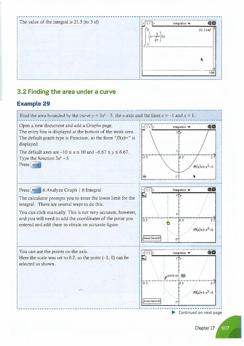
The value of the integral is 21.5 (to 3 sf)

3.2 Finding the area under a curve

Example 29

!fulc. Integration •

J}-t} tmm

21.5147 liSl

~

l!2l 1199

Find the area bounded by the curve y = 3x2 - 5, the x-axis and the lines x = -1 and x = 1.

Open a new document and add a Graphs page. The entry line is displayed at the bottom of the work area. The default graph type is Function, so the form ''fl(x)=" is displayed.

The default axes are - 10 ~ x ~ 10 and-6.67 ~ y ~ 6.67. Type the function 3x2 - 5

Press menu 6:Analyze Graph I 6:Integral

The calculator prompts you to enter the lower limit for the integral. There are several ways to do this.

You can click manually. This is not very accurate, however, and you will need to add the coordinates of the point you entered and edit them to obtain an accurate figure.

You can use the points on the axis. Here the scale was set to 0.2, so the point (-1, 0) can be selected as shown.

Integration •

7 y

,:

·2. 5 2.5

> ·7

Integration ...,

7 y

I 1

·2. 5

~ .2 2.5

f1(x)--3·x2-s /

1itower boundj ·7 -Integration ,. t1iJID

7 y

. I lf point on @ ,J .. •t• • • ❖••·$• .. }•••t•••~ .. ' •••••••I••• ❖ • • ❖ .. • • • • l ••• l • •• ❖ •••l• • •l•••t• • • ❖ ••• $• .. J•••I••• ❖ ••'?( ·2.5 . . 2 2. 5

\ f1(x)=3·x2-s

·7


Chapter 17

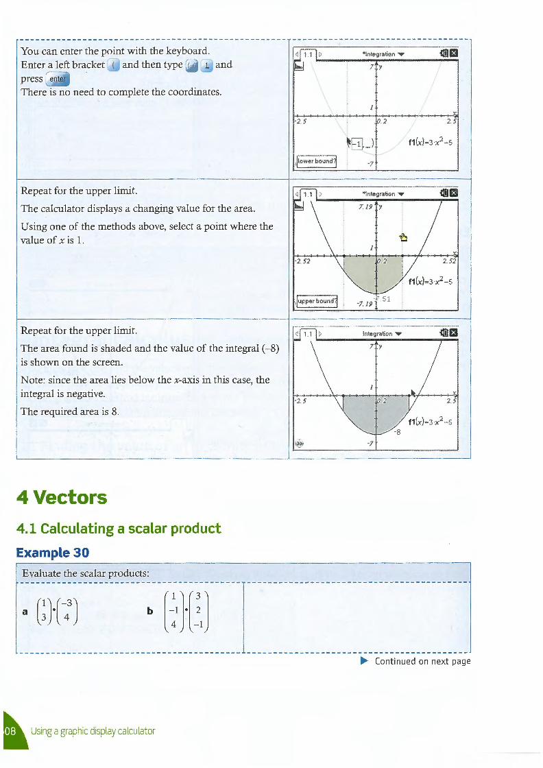
You can enter the point with the keyboard. Enter a left bracket ( and then type (-) 1 and press enter

There is no need to complete the coordinates.

Repeat for the upper limit.

The calculator displays a changing value for the area.

Using one of the methods above, select a point where the value of x is 1.

Repeat for the upper limit.

The area found is shaded and the value of the integral (-8) is shown on the screen.

Note: since the area lies below the x-axis in this case, the integral is negative.

The required area is 8.

4 Vectors

4.1 Calculating a scalar product

Example30

Evaluate the scalar products:


*Integration ,...

7 y

-2.5 . 2 2.5

~ED-) 1jlower bound~ _7

*Integration ,...

X

·2.52 2.52

Integration ,...

7 y

-2. 5

-7·


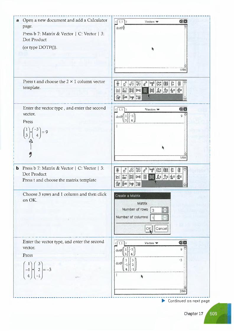
a Open a new document and add a Calculator page.

Press b 7: Matrix & Vector I C: Vector I 3: Dot Product

(or type DOTP()).

Press t and choose the 2 x 1 column vector template.

Enter the vector type , and enter the second vector.

Press

b Press b 7: Matrix & Vector I C: Vector I 3: Dot Product Press t and choose the matrix template

Choose 3 rows and 1 column and then click

on OK.

Enter the vector type, and enter the second vector.

Press

[-J[ _;J=-3

j,,l._> ____ v e_c_tor_s _ ... _____ «m_•"ffla dotP(j) ~

g Do .fo Vo lol go•~• (ggJ [co]

~ /§do Jc>j! ~'ffi

jul✓

dotP([ ~ l (-: ]) I

Create a Matrix

0199

lagO {o,o {11-g {" {g ~ o o,o ito D O ~

::: i O -fro d O dZo ~-n •=• •=• da Ta

~

"Vectors • «ma 9 ~

~

lYl 11'99

Matrix

Number of rows j 3 ;:::;;::=;;;:;:=;

Number of columns ... I 1_1 __ _.

jul> Vectors ,.

dotP([ ~ l[: ]) do~rnm I ~

··----· -

«ma 9 12\l

-3

lYl 21'99


Chapter 17

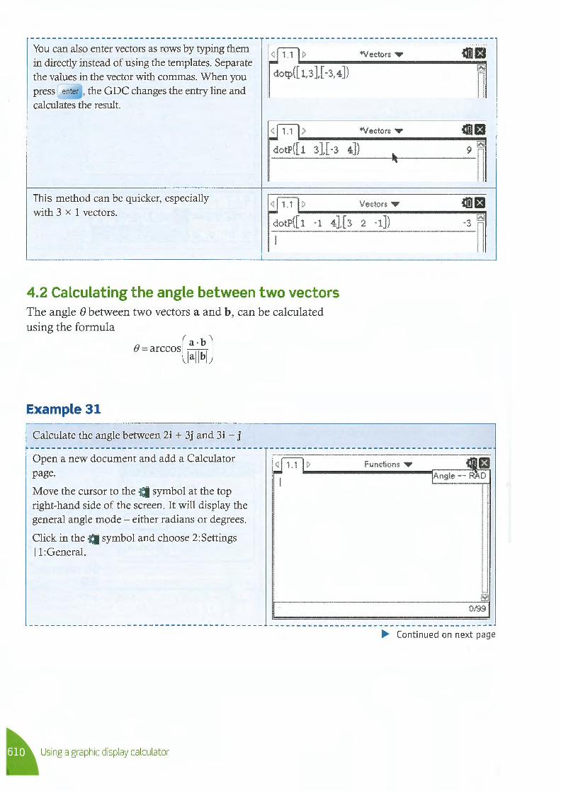
You can also enter vectors as rows by typing them in directly instead of using the templates. Separate the values in the vector with commas. When you press enter , the GDC changes the entry line and calculates the result.

dotp([ 1,3 ],[-3, 4])

dotP([ 1 3 l[-3 4])

>l'Vectors,..

>l'Vectors •

9 ~

Vectors • This method can be quicker, especially with 3 x 1 vectors.

dotP([ 1 · 1 41[ 3 2 · 1])

I ·3 ~

4.2 Calculating the angle between two vectors The angle 0 between two vectors a and b, can be calculated using the formula

(a-bl 0 = arccosllallbl

Example31

Calculate the angle between 2i + 3j and 3i - j


Move the cursor to the d symbol at the top right-hand side of the screen. It will display the general angle mode - either radians or degrees.

Click in the ~ symbol and choose 2:Settings 11 :General.


jul> I

Functions • f_g 1Angle -- RAD

0/99


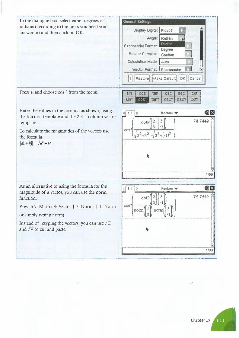
In the dialogue box, select either degrees or radians ( according to the units you need your answer in) and then click on OK.

Pressµ and choose cos-1 from the menu.

Enter the values in the formula as shown, using the fraction template and the 2 x 1 column vector template.

To calculate the magnitudes of the vectors use the formula [ai + bj[= ✓a2 +b2

As an alternative to using the formula for the magnitude of a vector, you can use the norm function.

Press b 7: Matrix & Vector I 7: Norms I 1: Norm

or simply typing norm(

Instead of retyping the vectors, you can use / C and / V to cut and paste.

General Settings


Angle:

Exponential Format:

Real or Complex: Gradian 1------L--~

Calculation Mode: Auto ::::===== ::::::::::.::::.::::.::::..::..::;'

Vector Format: I Rectanoular

[ii I Resto rel I Make Default! I OK 11 Cancetl

sin

sin-'

tan csc sec cot

tan-1 csc-1 sec·1 cot1

~ > Vectors ,.. «mm

coo{~[J~LJllJ2) 74.7449 ~

1/99

~ > Vectors • «m £f

dotP([ ~ }[ _31 ]) 74.7449 ~

cos·' nonn([ ~ ]) · nonn([ _31 ])

~

Isa 1/99

Chapter 17

5 Statistics and probability You can use your GDC to draw charts to represent data and to calculate basic statistics such as mean, median, etc. Before you can do this, you need to enter the data into a list or spreadsheet. This is done in a Lists & Spreadsheet page in your document.

Entering data There are two ways of entering data: as a list or as a frequency table.

5.1 Entering lists of data

Example 32

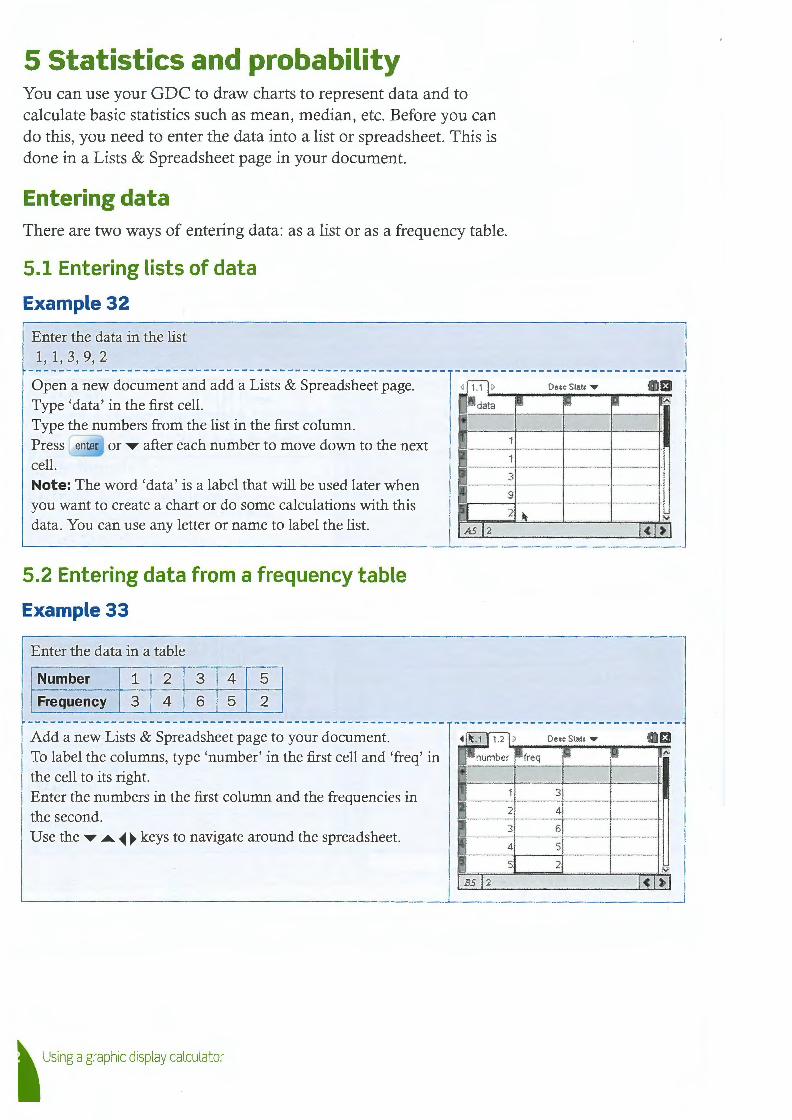
Enter the data in the list 1,1,3,9,2

Open a new document and add a Lists & Spreadsheet page. Type 'data' in the first cell. Type the numbers from the list in the first column. Press enter or ....,. after each number to move down to the next cell. Note: The word 'data' is a label that will be used later when you want to create a chart or do some calculations with this data. You can use any letter or name to label the list.

5.2 Entering data from a frequency table

Example33

Enter the data in a table

Number 1 2 3 4 5

Frequency 3 4 6 5 2

Add a new Lists & Spreadsheet page to your document.

< r,:-i7 > '" [IS data

I• 11

AS 12

Desc Stats ,..

Ill !iii

1

1

3 --9

2 ~

Desc Slats ,..

To label the columns, type 'number' in the first cell and 'freq' in the cell to its right.

• c!.1 .21> • number !ll freq g

Enter the numbers in the first column and the frequencies in the second. Use the ....,. ... • • keys to navigate around the spreadsheet.


•

~

I<

B5 12

1 3

2 4

3 6

4 5

5 2

ma y 211

lS!i

l<l>I

ma !I ii:ll

-~

l< l >I

Drawing charts You can draw charts from a list or from a frequency table.

5.3 Drawing a frequency histogram from a list

Example 34

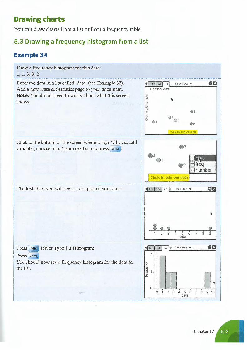
Draw a frequency histogram for this data: 1, 1, 3, 9, 2

Enter the data in a list called 'data' (see Example 32). Add a new Data & Statistics page to your document. Note: You do not need to worry about what this screen shows.

Click at the bottom of the screen where it says 'Click to add variable', choose 'data' from the list and press enter .

The first chart you will see is a dot plot of your data.

Press menu 1:Plot Type I 3:Histogram

Press enter

You should now see a frequency histogram for the data in the list.

• 1.1 1.2 1.3 1.,,,_ oe-•c_s_1at-• _ ..... ___ .;;.;£1;;.

Caption: data

0 3

0 9

Click to add va11able

[Id ta 0 9 {"•} freq I

{u-} number I

I Click to add variable

• 1.1 1.2 1.3 > Desc Stats ,... f3

0 0 0 0 0 1 2 3 4 5 6 7 8 9

data

• 1.1 1.2 1.3 > Desc Stats ,... f3

2

>, u C <I) :, g- 1 t.t

~ 0

0 1 2 3 4 5 6 7 8 9 10 data

Chapter 17

5.4 Drawing a frequency histogram from a frequency table

Example 35

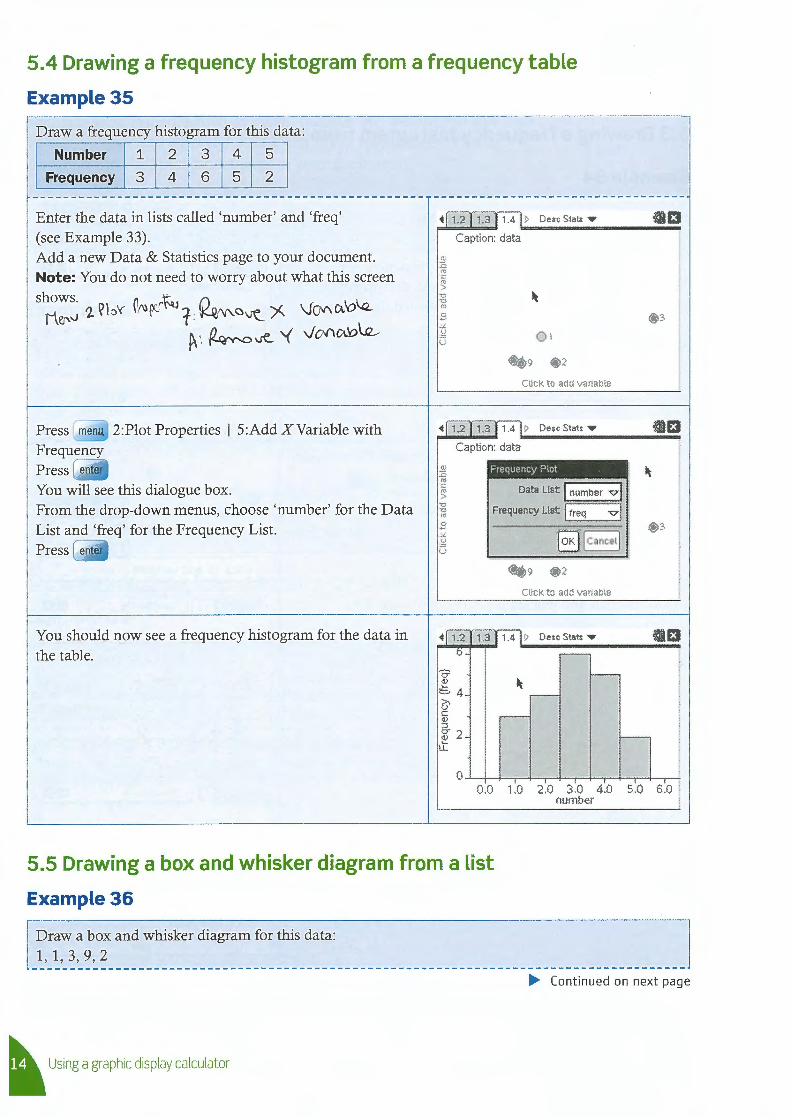
Draw a frequency histogram for this data:

Number 1 2 3 4 5

Frequency 3 4 6 5 2

Enter the data in lists called 'number' and 'freq' (see Example 33). Add a new Data & Statistics page to your document. Note: You do not need to worry about what this screen

shows. ~ ~ n \.a.. Mei--.v 2 ~bY )".)fQ r: ~l\f\.Cv~ )(. \J(rv'\CA.YJ

~ '. ~ -se.. '{ '1 (Jl'l@\.Q_,,

2:Plot Properties I 5:Add XVariable with

Press enter

You will see this dialogue box. From the drop-down menus, choose 'number' for the Data List and 'freq' for the Frequency List.

You should now see a frequency histogram for the data in the table.

• 1.2 1.3 1 .4 !> Oesc Stats ..., 13 '--------....,;~ Caption: data

0 3

Q:)9 0 2

Click to add variable

• 1.2 1.3 1.4 !> OescStats ,.. 13 .... ______ ....,;__, Caption: data

Frequency Plot

Data List ! number v !

Frequency List I freq vi

§) !cancel!

0 3


0.0 1,0 2.0 3.0 4,0 5.0 6.0 number

5.5 Drawing a box and whisker diagram from a list

Example36

Draw a box and whisker diagram for this data: 1, 1, 3, 9, 2



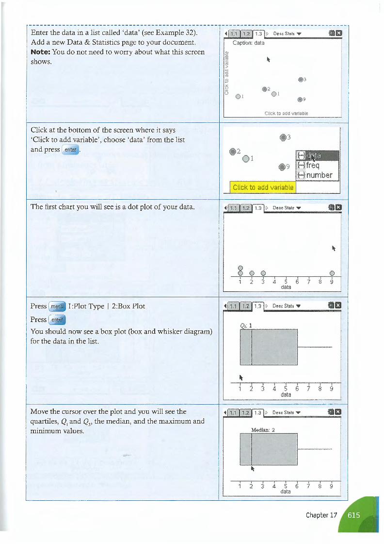
Enter the data in a list called 'data' (see Example 32). Add a new Data & Statistics page to your document. Note: You do not need to worry about what this screen shows.

Click at the bottom of the screen where it says 'Click to add variable', choose 'data' from the list

The first chart you will see is a dot plot of your data.

Press 1 :Plot Type I 2:Box Plot

Press

You should now see a box plot (box and whisker diagram) for the data in the list.

Move the cursor over the plot and you will see the quartiles, Q

1 and Q

3, the median, and the maximum and

minimum values.

• 1.1 1.2 1.3 :> Oesc Stats .,.. £1 -----------Caption: data

!B

~ ~ ~ "C "C

"' .s Y. t.)

"" u 0 1

0 2 0 1

0 3

0 9


0 3

Ill d1. .a 0 2 0 1

0 9 {u•} freq { .. ·}number


• 1.1 1.2 1.3 ;> Oesc Stats .,.. £1 ----------'""'!

0 0 0 0 0 1 2 3 4 5 6 7 8 9

data

• 1.1 1.2 1.3 ~ Desc Stats T £1

Q1: 1

I I ~

2 3 4 5 6 7 8 9 I data

• 1.1 1.2 1.3 ;> Oesc Stats .,.. £1

Median: 2

I I ~

2 3 4 5 6 7 8 9 I data

Chapter 17

5.6 Drawing a box and whisker diagram from a frequency table

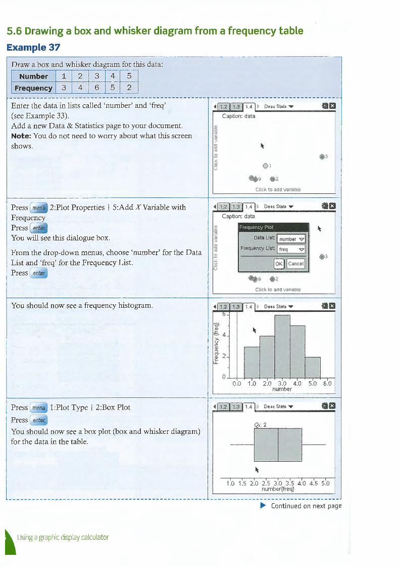
Example37

Draw a box and whisker diagram for this data:

Number 1 2 3 4 5

Frequency 3 4 6 5 2

Enter the data in lists called 'number' and 'freq' (see Example 33). Add a new Data & Statistics page to your document. Note: You do not need to worry about what this screen shows.

2:Plot Properties I 5:Add XVariable with

Press enter

You will see this dialogue box.

From the drop-down menus, choose 'number' for the Data List and 'freq' for the Frequency List.

You should now see a frequency histogram.

Press

Press

1 :Plot Type I 2:Box Plot

You should now see a box plot (box and whisker diagram) for the data in the table.


• 1.2 1.3 1.4 :> De sc Stats ..., 13 .._ __________ _

Caption: data

Q)

:0 "' ~ > :g lit "' .8 X.

~ 0 1 u (b9 0 2


• 1.2 1.3 1.4 > DescStats ..- 13 .._ ________ _, Caption: data

Frequency Plot

Data List: l number v!

Frequency List j freq vi

E)!cancel]


0 ..J...._+-+--..--f--r-+--,--+---.---1-.....---+-..--l 0.0 1.0 2.0 3 .0 4.0 5.0 6.0

number

• 1.2 1.3 1.4 !> Desc Stats ..- £1 '-----------•-

1.0 1.5 2.0 2.5 3 .0 3 .5 4.0 4.5 5.0 number{freq}


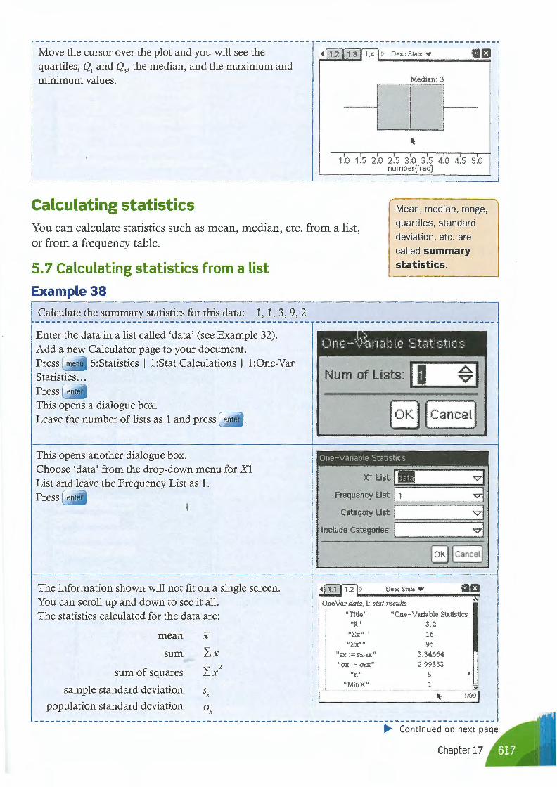
Move the cursor over the plot and you will see the quartiles, Q

1 and Q

3, the median, and the maximum and

minimum values.

Calculating statistics

• 1.2 1.3 1 .4 > Desc Stats ..,, £1

Median: 3

-----ll II -1.0 1.5 2 .0 2.5 3.0 3.5 4 .0 4.5

number{freq} 5.0 I

You can calculate statistics such as mean, median, etc. from a list, or from a frequency table.

Mean, median, range,

quartiles, standard

deviation, etc. are

called summary statistics. 5.7 Calculating statistics from a list

Example38

Calculate the summary statistics for this data: 1, 1, 3, 9, 2

Enter the data in a list called 'data' (see Example 32). Add a new Calculator page to your document.

1:Stat Calculations I 1:0ne-Var

Press enter

This opens a dialogue box. Leave the number of lists as 1 and press

This opens another dialogue box. Choose 'data' from the drop-down menu for X1 List and leave the Frequency List as 1.

The information shown will not fit on a single screen. You can scroll up and down to see it all. The statistics calculated for the data are:

mean

sum

sum of squares

sample standard deviation

population standard deviation

X

s X

(J' X

') - - ', S- .· . 1• t- •:--t.-t· ,-·t · ~ .~ lJ tl>=-- \I dtl.31.t ~ .:: . . d .I .:, .I L .:,

Num of Lists:

_o_K_ I Cancel j

X1 List II v! '::======== Frequency List vi

:==========~ Category List vi

:=:=======: Include Categories: ,__ ______ v....,I

Desc Stats ..,, f3 One Var data, 1: stat.results

"Title " "One- Variable Statistics 11x11 3.2

.. Z::x" , 16. 11z::x: 11 96.

11SX :== Sn- u:: 11 3.34664

110X := OnX 11 2.99333 1/nll 5.

"MinX" 1. M ~ 1199

• Chapter 17

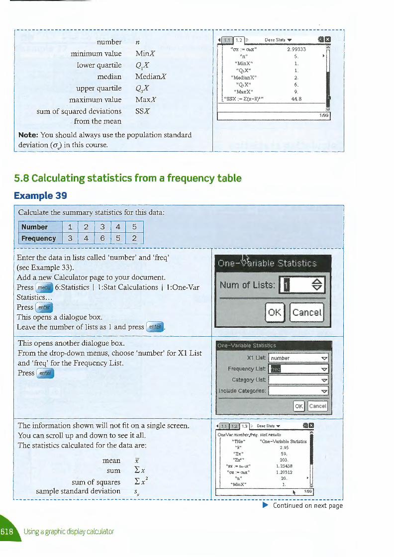
number

minimum value

lower quartile

median

upper quartile

maximum value

sum of squared deviations from the mean

n

MinX

Q,X

MedianX

Q3X

MaxX

SSX

Note: You should always use the population standard deviation ( a) in this course.

11ox := anX '1

•• n"

"MinX " "Q,X"

"MedianX" "QJX II

11MaxX 11

"SSX :~ L'.(x-x)'"

Desc Slats • £1 2.99333

5.

1.

1.

2. 6.

9. 44.8

1/99

5.8 Calculating statistics from a frequency table

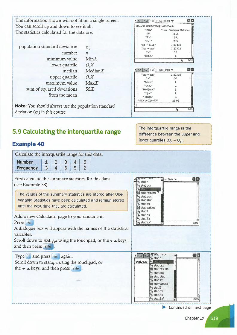
Example39

Calculate the summary statistics for this data:

Number 1 2 3 4 5

Frequency 3 4 6 5 2

Enter the data in lists called 'number' and 'freq' (see Example 33). Add a new Calculator page to your document. Press menu 6:Statistics I 1:Stat Calculations I 1:0ne-Var Statistics ... Press enter

This opens a dialogue box. Leave the number of lists as 1 and press

This opens another dialogue box. From the drop-down menus, choose 'number' for XI List and 'freq' for the Frequency List.


mean x sum LX

sum of squares LX 2

sample standard deviation s X


0 • - •• ,\.. . r l• I •;:'t r t· r- t · - 0:t f I;:! - v •,:H Id lJ .8 ._\ .d .I.:, .I!_. ._,

Num of Lists: _I a __ ~_-_I

;_O_K_ [cancetj

One-Varral)le Stat,strcs

X1 List I number vi

Frequency List ! Ill v j ~ ======= Category List I vi

:========: Include Categories: l.__ _ _ ____ v...,I

• 1 1 1.2 1.3 ~ De•e Stat< .,.. El ....._ ______ .,..,.i;s

One Var number freq: stat.results

"Title " "One- Variable Statistics

"x" 2.95 "Z:x " 59 .

11 :Ex" " "sx :• Sn•1X"

"ox :a OnX "

llnll

11 MinX "

203 . 1. 23438 1. 203 12

20 . 1.

1/99



population standard deviation

number minimum value

lower quartile median

upper quartile maximum value

sum of squared deviations from the mean

(J X

n

MinX

QIX MedianX

Q3X MaxX ssx

Note: You should always use the population standard deviation ( cr) in this course.

5.9 Calculating the interquartile range

Example40

Calculate the interquartile range for this data:

Number 1 2 3 4 5 Frequency 3 4 6 5 2

First calculate the summary statistics for this data (see Example 38).

( The values of the summary statistics are stored after One- '

Variable Statistics have been calculated and remain stored

until the next time they are calculated.

Add a new Calculator page to your document. Press var

A dialogue box will appear with the names of the statistical variables. Scroll down to stat.q

3x using the touchpad, or the .... ...._ keys,

and then press enter .

-

• 1.1 1.2 1.3 ~ De•c Stats • £1 --------RS""'-OneVar ,rumber freq : stat.results

•

I

"Title" "One- Variable Statistics "x" 2.95

"Ex " 59 . "Ex2 11 203.

"sx :- Sn- 1X 11

tlox :• Q'nX B

"n" "Min X"

1.1 IP-2 1 u 1~ 110X :""'OnX 11

llfill

"Min X" "Q, X"

"MedianX" "Q,X "

"MaxX " "SSX :• :1:(x - x)' "

1.23438 1. 203 12

20. 1.

Oe$C Stat$ ..,.

1.203 12 20. 1. 2. 3 . 4. 5 .

28.95

~

1199

ma ~

•

51i 1199 I

The interquartile range is the

difference between the upper and

lower quartiles (Q3

- Q1

).

13

0/99

0/99


Chapter 17

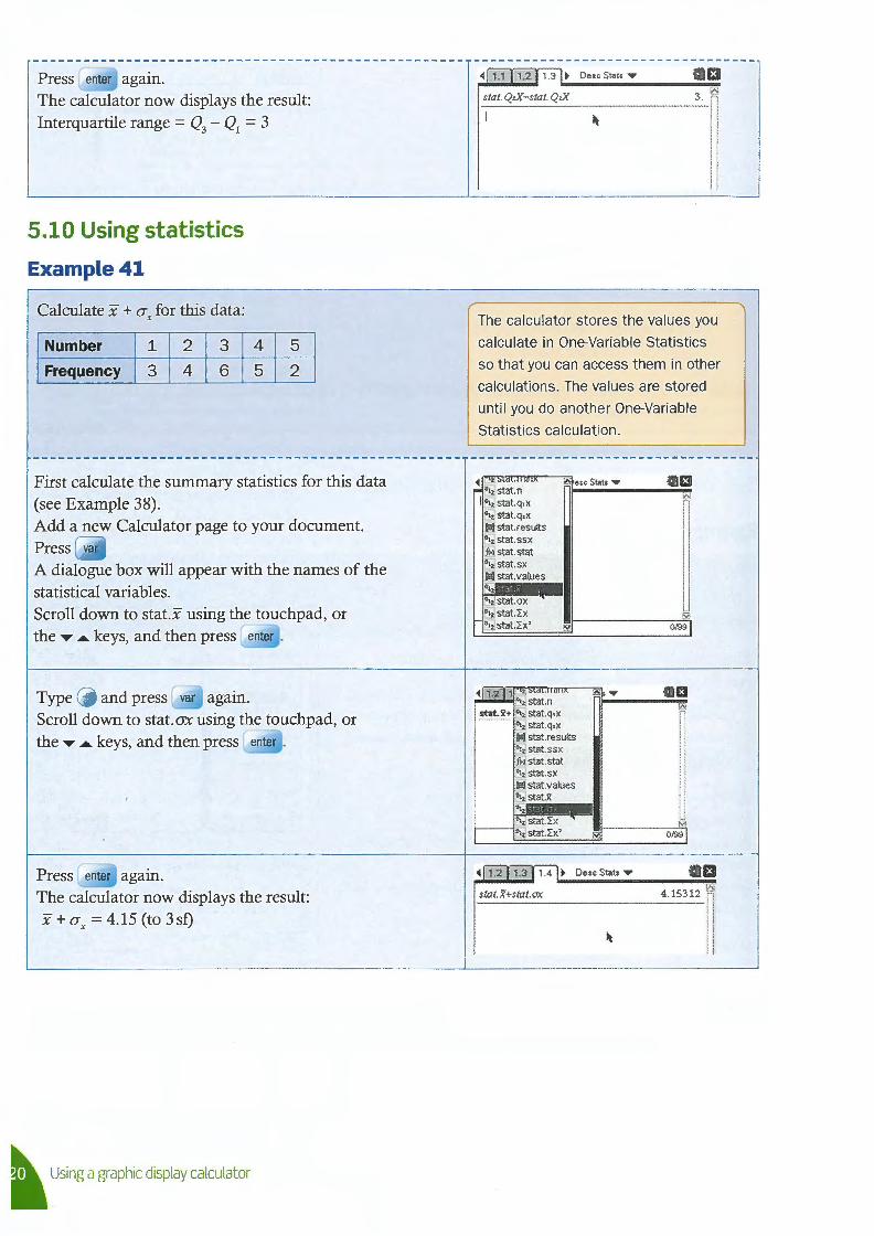
Press enter again. The calculator now displays the result: Interquartile range= Q3 - Q1 = 3

5.10 Using statistics

Example41

Calculate .x + a-x for this data:

Number 1 2 3

Frequency 3 4 6

4

5

5

2

First calculate the summary statistics for this data (see Example 38). Add a new Calculator page to your document. Press var

A dialogue box will appear with the names of the statistical variables. Scroll down to stat..x using the touchpad, or the ..., .... keys, and then press enter .

Type -f and press var again. Scroll down to stat. ax using the touch pad, or the ....- .... keys, and then press enter .

Press enter again. The calculator now displays the result: x + a-x = 4.15 (to 3sf)


• 1.1 1.2 1.3 • Desc Stats• £J __________ ..;;;,; stat. Q,X- stat. Q.X 3. l!Sl

The calculator stores the values you

calculate in One-Variable Statistics

so that you can access them in other

calculations. The values are stored

until you do another One-Variable

Statistics calculation.

13

0/99

GD

0/99

• 1.2 1.3 1.4 • De•c Stats • £J -------------stat.x+stat.ax 4 lS 312 ~

Calculating binomial probabilities

5.11 The use of nCr

Example42

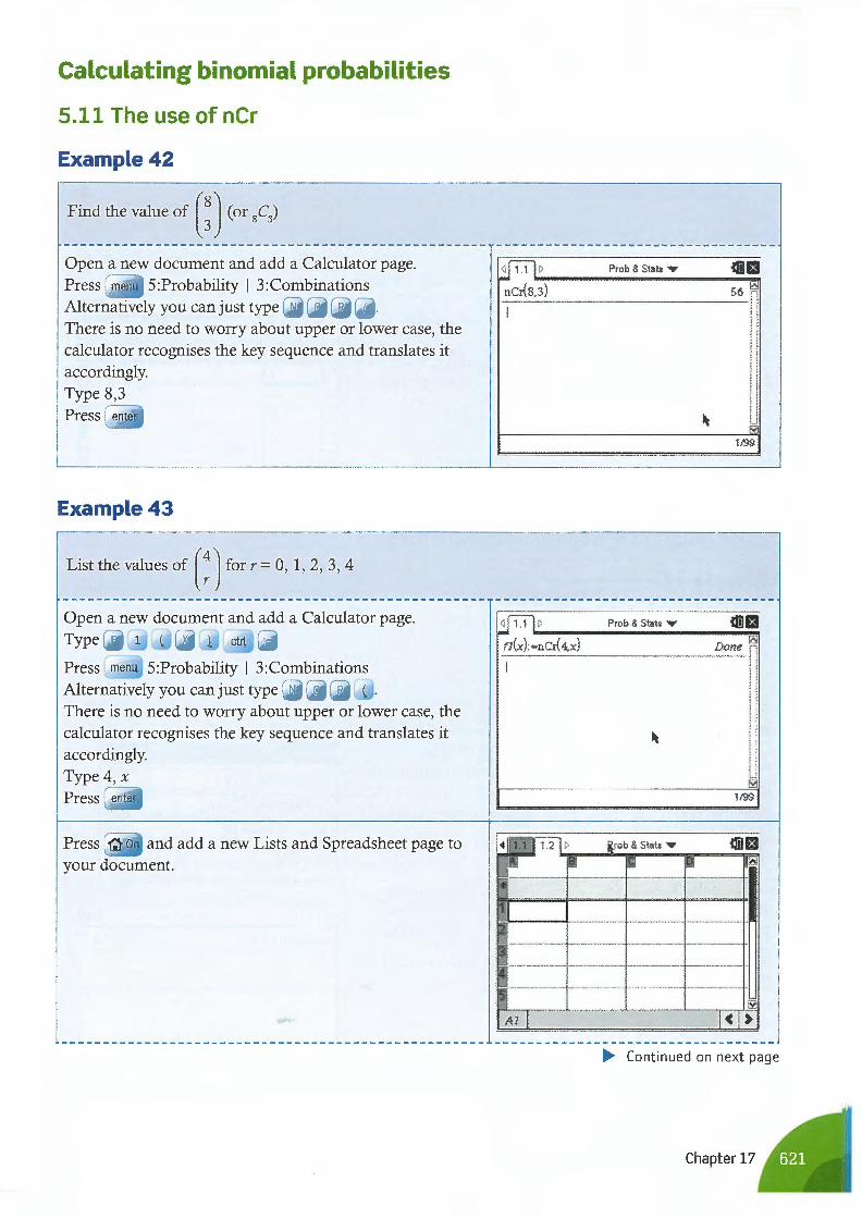
Find the value of(:) (or 8C,)

Open a new document and add a Calculator page. Press menu 5:Probability I 3:Combinations Alternatively you can just type N c R ( .

There is no need to worry about upper or lower case, the calculator recognises the key sequence and translates it accordingly. Type 8,3

Example43

List the values of [: 1 for r = 0, 1, 2, 3, 4

Open a new document and add a Calculator page. Type F ( )

Press menu 5:Probability I 3:Combinations Alternatively you can just type N c R ( •

There is no need to worry about upper or lower case, the calculator recognises the key sequence and translates it accordingly. Type 4, x

Press ~ On and add a new Lists and Spreadsheet page to your document.

~ > ncr(s,3)

I

jul> fl(x) : =ncr( 4,x)

I

• ~ 1.2j > .. !I

I•

1

I AJ I

Prob & Stat$ ,.. oa 56 l1Sl

~ fS1j

1199

Prob & Stab,.. oa Done

l1Sl

~

fS1j

1199

irob & Stal$ ,.. 4lil£1 g !I ~

.

.

~

i


Chapter 17

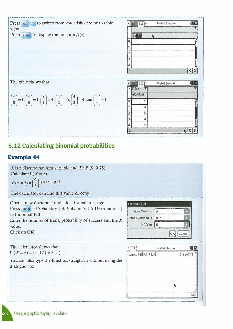
Press view. Press

T to switch from spreadsheet view to table

to display the functionfl(x)

The table shows that

( ~ )= 1, (~)=I, ( ~ )= 4, ( ~ )= 6, (: )= 4 and ( ! )= 1

5.12 Calculating binomial probabilities

Example44

Xis a discrete random variable and X ~ B (9, 0. 7 5) Calculate P( X = 5)

P(x=5)=(:)o.755 0.254

The calculator can find this value directly

Open a new document and add a Calculator page. Press menu 5:Probability I 3:Probability I 5:Distributions I D:Binomial Pdf... Enter the number of trials, probability of success and the X value. Click on OK

The calculator shows that P (X= 5) = 0.117 (to 3 sf)

You can also type the function straight in without using the dialogue box.

t. Using a graphic display calculator

!i ~1.2j > Prob & Stats ..- iD.1£1 T

~ ~ 0.

i 1.

2.

3.

4. 51

l

0.

1

2 3. 4.

1

1.

4 .

6.

1.

Binomial Pdf

Num Trials, n: 19 :========:

Prob Success, p: I 0.75 :=======:::;

X Value: I sj

< 1.17 > Prob & Stats ..- iD.1£1 binomPdr( 9,0 . 75,5) 0. 116798 12\l

~

~ 1199

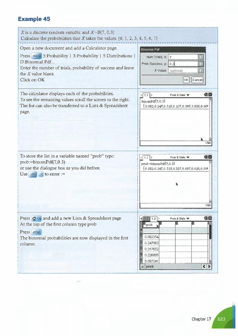
Example45

Xis a discrete random variable and X ~B(7, 0.3) Calculate the probabilities that Xtakes the values {O, 1, 2, 3, 4, 5, 6, 7}


Press menu 5:Probability I 3:Probability I 5:Distributions I D:Binomial Pdf... Enter the number of trials, probability of success and leave the X value blank. Click on OK

The calculator displays each of the probabilities. To see the remaining values scroll the screen to the right. The list can also be transferred to a Lists & Spreadsheet page.

To store the list in a variable named "prob" type: prob:=binomPdf(7,0.3) or use the dialogue box as you did before.

Press ~ On and add a new Lists & Spreadsheet page At the top of the first column type prob

Press enter

The binomial probabilities are now displayed in the first column.

Binomial Pdf

Num Trials, n: j 7 I ;:=;:::=====;:::::;

Prob Success, p: Io.~ J ! ~=====~~ X Value: j (optional) I

~~ Prob & Stats...,. «mm binomPdf17,0.3)

{ 0.082,0. 247,0.318, 0 .227,0.097,0 .025,0.00•

11-------------~~ 1199

~ :> Prob & Stats ..,. «mm prob: =binomPdr( 7, 0 . 3) ~

{ 0.082,0 .247,0.318,0.227, 0.097,0.025,0 .00•

~

fS1l 1/99

• .!:.!.J 1.2 1 > Prob & Stats ...,. «mm :3 prob t\- El !:I ~ ~

-4

0.082354

0.247063 -

0.317652

0.226895

0.097241

I prob l

Chapter 17

.,.

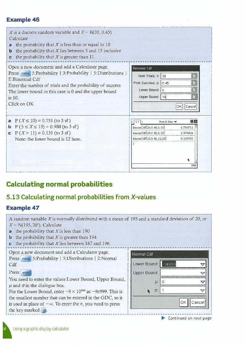
Example46

Xis a discrete random variable and X ~ B(20, 0.45) Calculate a the probability that Xis less than or equal to 10 b the probability that X lies between 5 and 15 inclusive c the probability that Xis greater than 11

Open a new document and add a Calculator page. Press menu 5:Probability I 3:Probability I 5:Distributions I E:Binomial Cdf Enter the number of trials and the probability of success The lower bound in this case is O and the upper bound is 10. Click on OK

a P (X~ 10) = 0.751 (to 3 sf) b P (5 ~ X~ 15) = 0.980 (to 3 sf) c P (X> 11) = 0.131 (to 3 sf)

Note: the lower bound is 12 here.

Calculating normal probabilities

Binomial Cdf

Num Trials, n: i 20 :=======~

Prob Success, p: I 0.45 :=====::::;::~

Lower Bound: I o !=========;

Upper Bound: !._1 __ 01"--------

Prob & Stab T iliJ£f binomCdr(20,0 .45,0, l O) 0. 750711 ~ binomcdr(20, 0 . 45, 5, 15) 0 . 979606

binomCdr(20,0 .45, 12,20) 0.130765

I

3199

5.13 Calculating normal probabilities from X-values

Example47

A random variable Xis normally distributed with a mean of 195 and a standard deviation of 20, or X ~ N(l 95,202

). Calculate a the probability that Xis less than 190 b the probability that Xis greater than 194 c the probability that X lies between 187 and 196.

Open a new document and add a Calculator page. Press menu 5:Probability I 5:Distributions I 2:Normal Cdf

Press

You need to enter the values Lower Bound, Upper Bound, µ and CJ in the dialogue box. For the Lower Bound, enter - 9 x 10999 as - 9E999. This is the smallest number that can be entered in the GDC, so it is used in place of - 00 • To enter the E, you need to press the key marked E •


Normal Celt

Lower Bound: ~I ·~jp~p;~j======v;· JI Upper Bound: I vi

:=:======= µ: lo vi

:============~ ~ o: l..._, _____ v__.l


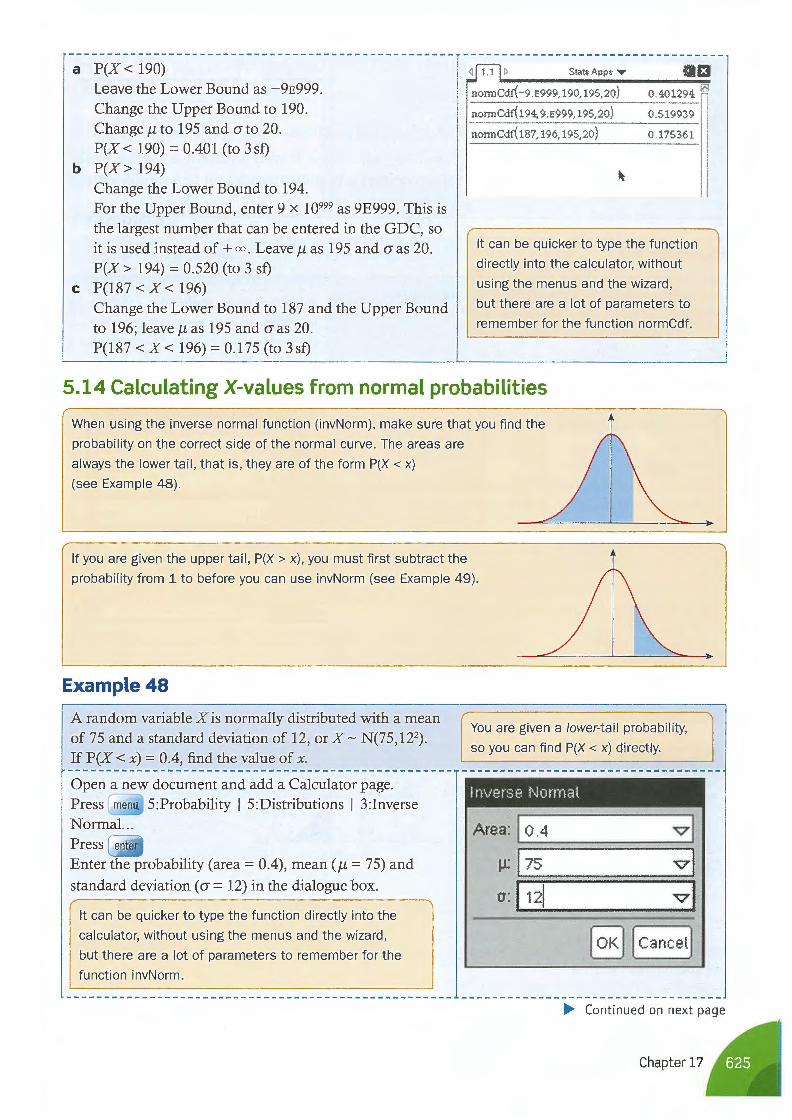
a P(X < 190) Leave the Lower Bound as -9E999. Change the Upper Bound to 190. Changeµ to 195 and ato 20. P(X < 190) = 0.401 (to 3 sf)

b P(X> 194) Change the Lower Bound to 194. For the Upper Bound, enter 9 x 10999 as 9E999. This is the largest number that can be entered in the GDC, so it is used instead of + oo. Leave µ as 19 5 and CJ as 20. P(X > 194) = 0.520 (to 3 sf)

c P(187 < X < 196) Change the Lower Bound to 187 and the Upper Bound to 196; leaveµ as 195 and CJ as 20. P(187 < X < 196) = 0.175 (to 3sf)

Stats Apps ,.. 13 normCdf(-9 E999, 190, 19S,20) 0. 401294 !!\l

normCdf(194, 9 .E999, 195,20) 0. 519939

no1mCdf(187, 196, 195, 20) 0.175361

It can be quicker to type the function

directly into the calculator, without

using the menus and the wizard,

but there are a lot of parameters to

remember for the function normCdf.

5.14 Calculating X-values from normal probabilities

When using the inverse normal function (invNorm), make sure that you find the

probability on the correct side of the normal curve. The areas are

always the lower tail, that is, they are of the form P(X < x)

(see Example 48).

If you are given the upper tail, P(X > x), you must first subtract the

probability from 1 to before you can use invNorm (see Example 49).

Example48

A random variable Xis normally distributed with a mean of 75 and a standard deviation of 12, or X ~ N(75, 122) .

If P(X < x) = 0.4, find the value of x.

Open a new document and add a Calculator page. 5:Probability I 5:Distributions I 3:Inverse

Press enter

Enter the probability (area= 0.4), mean(µ= 75) and

standard deviation (a= 12) in the dialogue box.

It can be quicker to type the function directly into the

calculator, without using the menus and the wizard,

but there are a lot of parameters to remember for the

function invNorm.

You are given a lower-tail probability, I so you can find P(X < x) directly.

Area: I 0.4 vi :::::===============:

µ: 175 vi

a: I 121 vi


Chapter 17

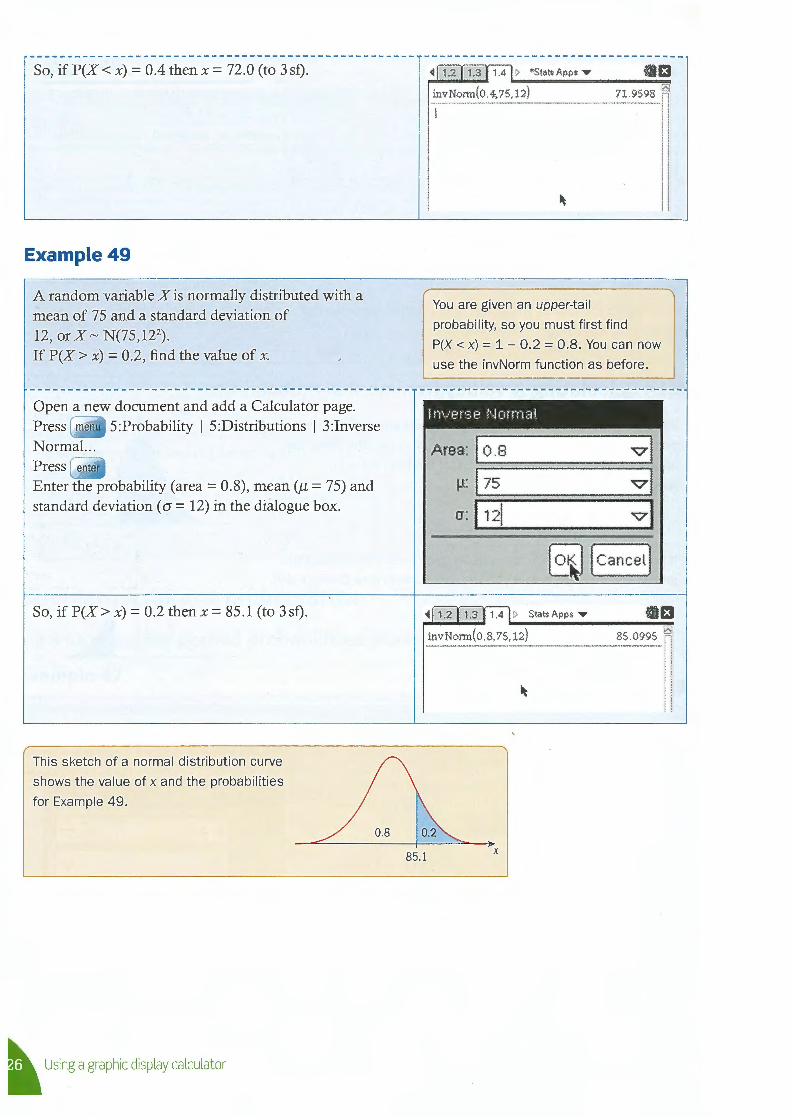
So, if P(X < x) = 0.4 then x = 72.0 (to 3 sf).

Example49

A random variable Xis normally distributed with a mean of 7 5 and a standard deviation of 12, or X ~ N(75, 122

).

If P(X > x) = 0.2, find the value of x.

Open a new document and add a Calculator page. 5 :Probability I 5 :Distributions I 3 :Inverse

Press enter

Enter the probability (area= 0.8), mean(µ= 75) and standard deviation (a-= 12) in the dialogue box.

So, if P(X > x) = 0.2 then x = 85. l (to 3 sf).

This sketch of a normal distribution curve

shows the value of x and the probabilities

for Example 49.


0.8

• 1.2 1.3 1 .4 > *Stats Apps ,. 13 ---------in v No rm (04,75, 12) 71. 9598 !!SJ

You are given an upper-tail

probability, so you must first find

P(X < x) = 1 - 0.2 = 0.8. You can now

use the invNorm function as before.

Inverse f\Jorrnal

Area: I 0 .8 ;::· ==================:::::

µ: 175 o: 1,21

• 1.2 1.3 1.4 > Stats Apps ,. 13 ---------!!!!!' invNonn(O 8,75, 12) 8S 0995 I

0.2

85.1 X

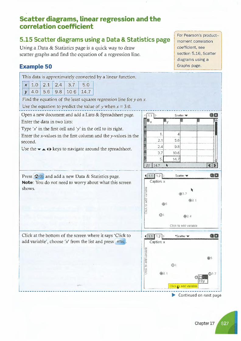
Scatter diagrams, linear regression and the correlation coefficient

5.15 Scatter diagrams using a Data & Statistics page Using a Data & Statistics page is a quick way to draw scatter graphs and find the equation of a regression line.

Example 50

This data is approximately connected by a linear function .

X 1.0 2.1 2.4 3.7 5.0 y 4.0 5.6 9.8 10.6 14.7

Find the equation of the least squares regression line for y on x.

Use the equation to predict the value of y when x = 3.0.

Open a new document and add a Lists & Spreadsheet page.

Enter the data in two lists:

Type 'x' in the first cell and 'y' in the cell to its right.

Enter the x-values in the first column and they-values in the second.

Use the ..- • • • keys to navigate around the spreadsheet.

Press ~ On and add a new Data & Statistics page. Note: You do not need to worry about what this screen shows.

Click at the bottom of the screen where it says 'Click to add variable', choose 'x' from the list and press

< --,.;-i > - '51

X Ji!jy -• 1 1,

2 2. 1

2.4

3,7

5,

B5 j14.7 ~

Caption: x

Q)

:0 !'.'1 ~ > u u "' os .8 Y. !,?

u O l

Caption: x

Q)

:0 "' ~ > u u "' .8 Y. u u 0 2 l

For Pearson's product

moment correlation

coefficient, see

section 5.16, Scatter

diagrams using a

Graphs page.

Scatter...- {[)£1 g !l 2S!

4

5.6

9,8 .

10.6

14.7

l

Scatter• El

~ 0 3 7

0 21

0 24

Click to add vanable

*Scatter• El

os O l

0 37

- Cltci' 'o adcl variable


Chapter 17

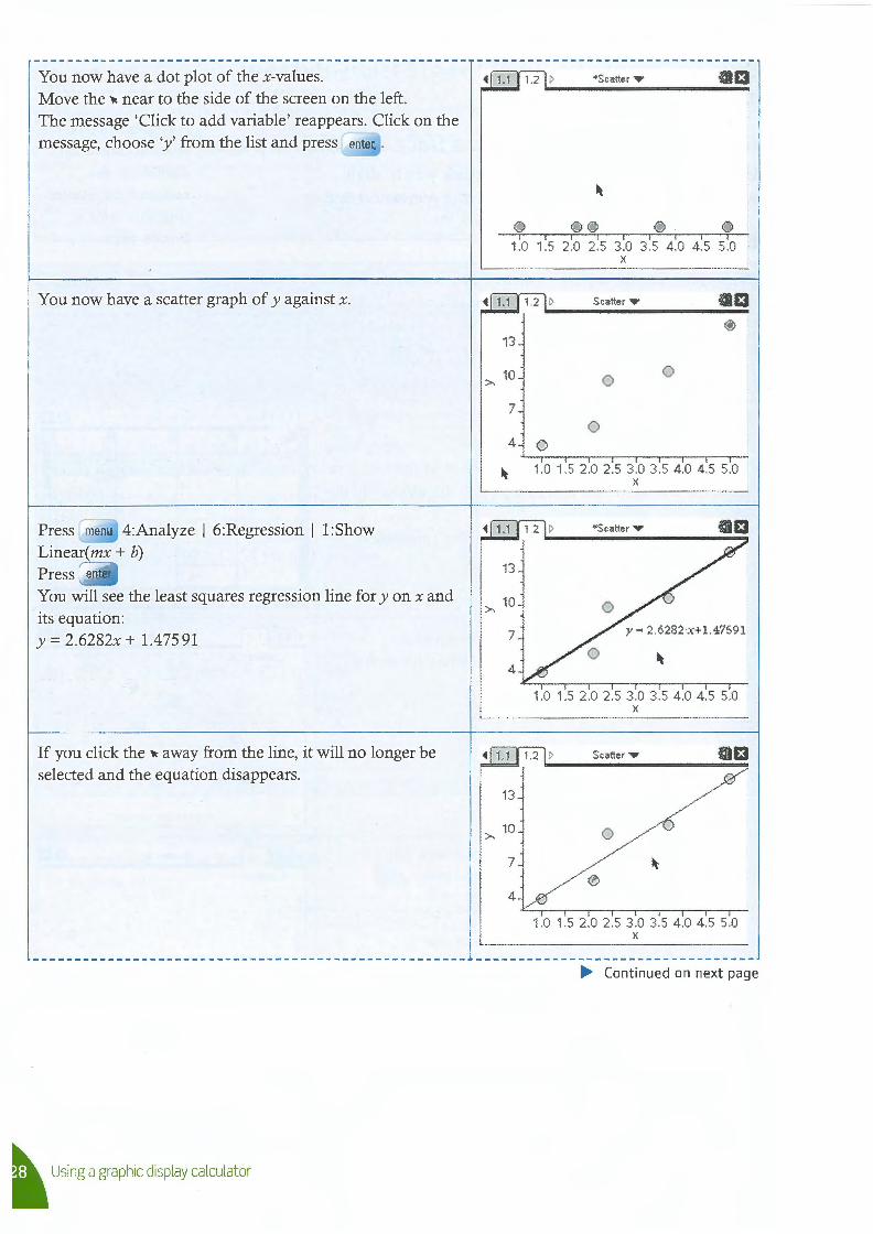
You now have a dot plot of the x-values. Move the ~ near to the side of the screen on the left. The message 'Click to add variable' reappears. Click on the message, choose 'y' from the list and press enter .

You now have a scatter graph of y against x.

Press menu 4:Analyze I 6:Regression I 1:Show Linear(mx + b) Press enter

You will see the least squares regression line for y on x and its equation: y = 2.6282x + I.475 91

If you click the ~ away from the line, it will no longer be selected and the equation disappears.


0 1.0

13

>- 10

7

4

13

>- 10

7

4

>.

13

10

7

4

*Scatter,.. 13

~

00 0 0 1.5 2.0 2.5 3.0 3.5 4.0 4.5 5.0

X

Scatter,.. 13 0

0 0

0 0

1.0 1.5 2.0 2.5 3.0 3 .5 4.0 4.5 5.0 X

*Scatter,..

y = 2.6282·x+ l.47S91

1.0 1.5 2.0 2.5 3.0 3.5 4.0 4.5 5.0 X

Scatter ,..

0

0

1.0 1.5 2.0 2.5 3.0 3.5 4.0 4.5 5.0 X


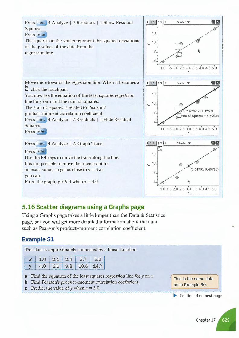
4:Analyze I 7:Residuals I 1 :Show Residual

Press enter

The squares on the screen represent the squared deviations of they-values of the data from the regression line.

Move the ~ towards the regression line. When it becomes a

0, click the touchpad. You now see the equation of the least squares regression line for y on x and the sum of squares. The sum of squares is related to Pearson's product-moment correlation coefficient.

4:Analyze I 7:Residuals I 1 :Hide Residual

Press

Press 4:Analyze I A:Graph Trace

Press Use the • • keys to move the trace along the line. It is not possible to move the trace point to an exact value, so get as close to x = 3 as you can. From the graph, y:::::: 9.4 when x = 3.0.

5.16 Scatter diagrams using a Graphs page

13

>- 10

7

4

13

>- 10

7

4

13

>- 10

7

4

Scatter-..

1.0 1.5 2 .0 2.5 3.0 3.5 4 .0 4.5 5.0 X

1.0 1.5 2.0 2.5 3.0 3.5 4 .0 4.5 5.0 X

*Scatter-..

1.0 1.5 2.0 2 .5 3.0 3 .5 4 .0 4.5 5.0 X

Using a Graphs page takes a little longer than the Data & Statistics page, but you will get more detailed information about the data such as Pearson's product-moment correlation coefficient.

Example51

This data is approximately connected by a linear function.

X 1.0 2.1 2.4 3.7 5.0 y 4.0 5.6 9.8 10.6 14.7

a Find the equation of the least squares regression line for y on x. b Find Pearson's product-moment correlation coefficient. c Predict the value of y when x = 3.0.

.( This is the same data I I as in Example 50.


Chapter 17

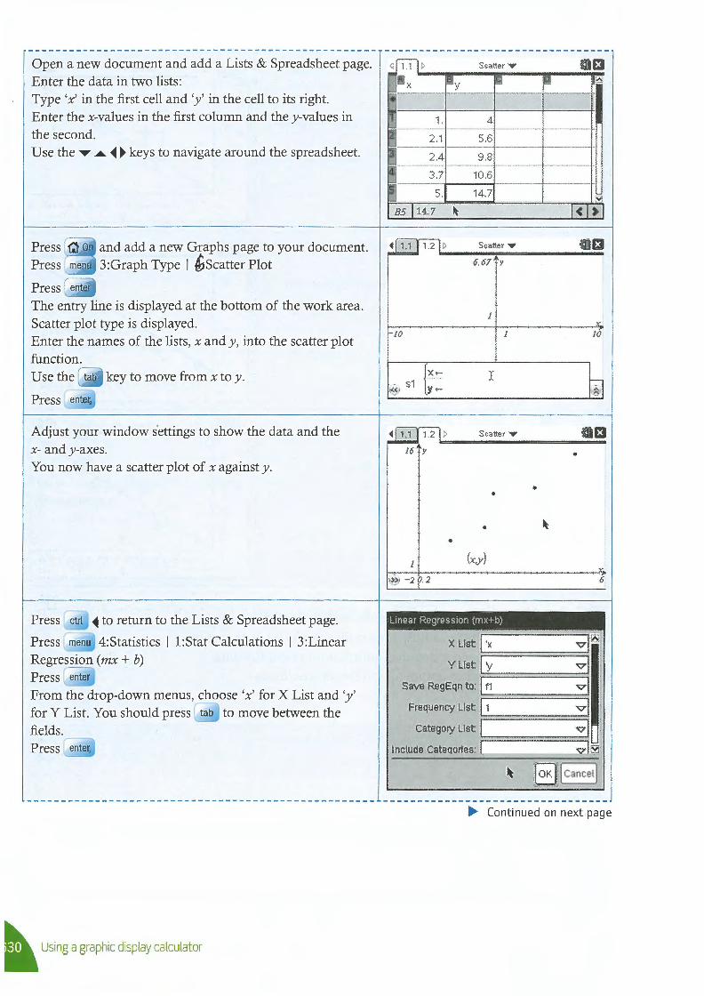
Open a new document and add a Lists & Spreadsheet page. Enter the data in two lists: Type 'x' in the first cell and 'y' in the cell to its right. Enter the x-values in the first column and they-values in the second. Use the ....,. ..._ • • keys to navigate around the spreadsheet.

Press ~ On and add a new Graphs page to your document. Press menu 3:Graph Type I 4iscatter Plot

Press enter

The entry line is displayed at the bottom of the work area. Scatter plot type is displayed. Enter the names of the lists, x and y, into the scatter plot function.

key to move from x toy.

Adjust your window s'ettings to show the data and the x- and y-axes. You now have a scatter plot of x against y.

Press ctrl • to return to the Lists & Spreadsheet page.

Press menu 4:Statistics I 1:Stat Calculations I 3:Linear Regression (mx + b) Press enter

From the drop-down menus, choose 'x' for X List and 'y' for Y List. You should press tab to move between the fields.


< 'T.,7 ,, Scatter,- ma • 29x !:!ly y !:I 2\l

• 1 1. 4

. 2.-1 5.6

2.4 9.8

~ 3.7 10.6

15 5. 14.7 Cl

BS I 14.7 1\- I< l>I

Scatter,. £1 6.67 y

X

-10 10

< s1 {;-: I

Scatter,.. £1 •

• •

• •

(x,y) .......... - ......... -----------......-,:.. ~ -2 0.2 6

Linear Regression (rn;:+tl)

X List: I ·x vi~ v ust: 1 y vi

Save RegEqn to: I f1 vi Frequency List: j 1 vi

Category List: I vi Include Cateqorles: I vi~

~ I OK J I Cancel]


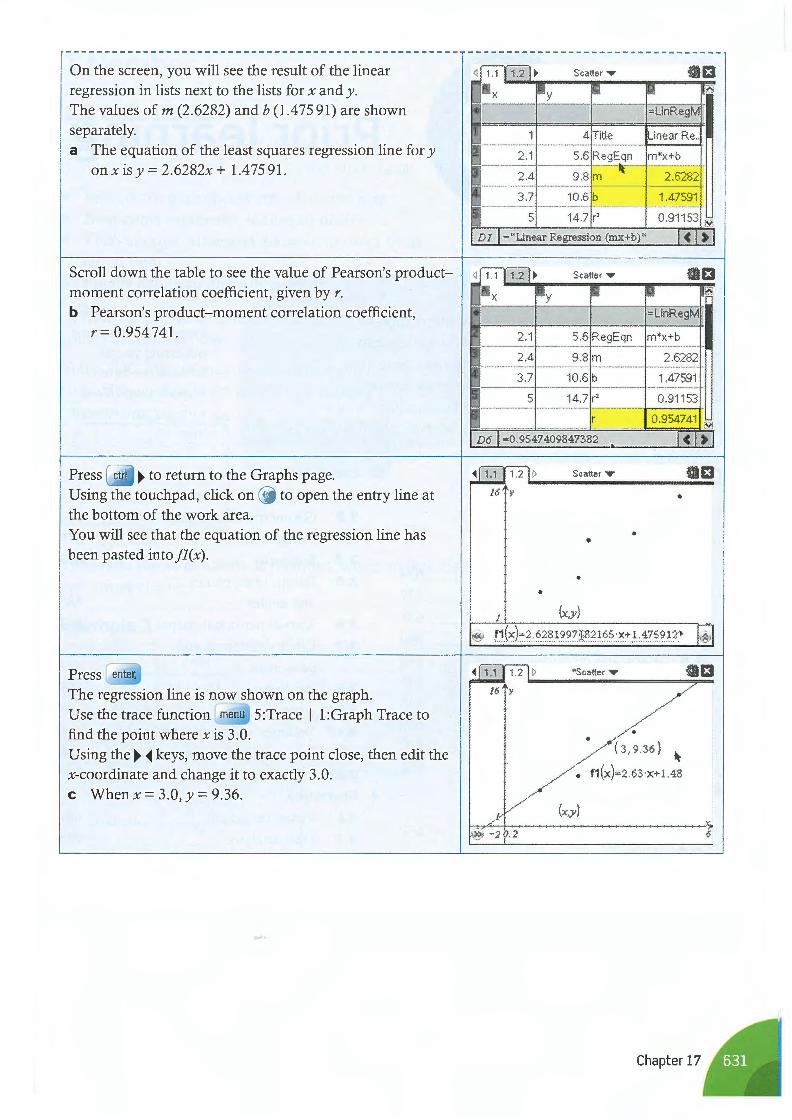
On the screen, you will see the result of the linear regression in lists next to the lists for x and y. The values of m (2.6282) and b (l.475 91) are shown separately. a The equation of the least squares regression line for y

on xis y = 2.6282x + l.475 91.

Scroll down the table to see the value of Pearson's productmoment correlation coefficient, given by r. b Pearson's product-moment correlation coefficient,

r = 0.954 741.

Press ctr! • to return to the Graphs page. Using the touch pad, click on < to open the entry line at the bottom of the work area. You will see that the equation of the regression line has been pasted into fl(x) .

Press enter

The regression line is now shown on the graph. Use the trace function menu 5:Trace I 1:Graph Trace to find the point where x is 3. 0. Using the • • keys, move the trace point close, then edit the x-coordinate and change it to exactly 3. 0. c When x = 3.0, y = 9.36.

~ 1.1 If 1.2 I• Scatter..,. {[}13 "' Rx !iy !) g !2Sl

• . =LinRegM

1 1 4 Title Linear Re .. ~ 2 .1 5.6 RegEqn m*x+b

3 2.4 9.8 If

2.6282 m

~ 3.7 10.6 b 1.47591 -5 5 14.7 r' 0.91153 ~

DI I • "Linear Regression (mx+b)" 1<1>

< 1.1 11 .2 I• Scatter..,. ffll3 : ~ x §IY g I.I

• I =LinRegM

2.1 5.6 RegEqn m*x+b

2.4 9 .8 m 2.6282

3.7 10.6 b 1.47591

15 5 14.7 r' 0.91153 ~

0.954741 r - - ~

D6 1-o. 9547409847382 l

1 .2 t> Scatter ..,. 13 ---------....;;~ •

• •

• •

(x,y)

1.2 :> *Scatter..,. -----------16 y

• • (3,9 .36) \

• f1(x)= 2. 63·x+l.48

Chapter 17

Documents

Graphing linear functions 572 Drawing a logarithmic graph