Gravity equations:Workhorse, toolkit, cookbook

Keith Head1,3 Thierry Mayer2,3,4

1Univ. of British Columbia, Sauder School of Business

2Sciences Po

3CEPR

4CEPII

National Bank of Belgium, November 21st, 2012.

Why you should not resist gravity

Gravity equations are a model of bilateral interactions in which sizeand distance effects enter multiplicatively.

They have been used as a workhorse for analyzing the determinantsof bilateral trade flows for 50 years.

Gravity is a tool for evaluating welfare impacts of trade policychanges.

Gravity also works for FDI, portfolio investment, tradable services,migration, tourism, even the internet.

“Physics envy”: Gravity is rare example in economics of “law-like”behavior.

Gravity research exemplifies the beneficent roles of empiricalregularities in guiding theory development and theory in guidingestimation.

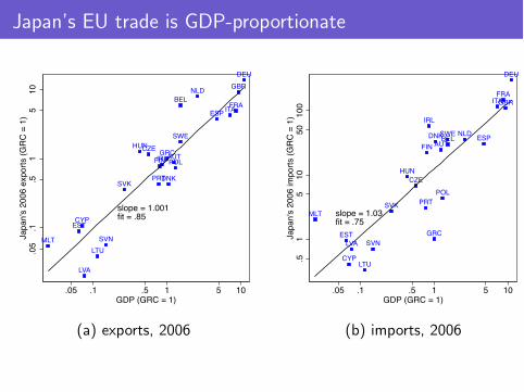
Japan’s EU trade is GDP-proportionate

MLT

ESTCYP

LVA

LTUSVN

SVK

HUNCZE

PRT

FINIRLGRC

DNK

AUTPOL

SWE

BELNLD

ESP ITAFRA

GBRDEU

slope = 1.001fit = .85

.05

.1.5

15

10Ja

pan'

s 20

06 e

xpor

ts (G

RC =

1)

.05 .1 .5 1 5 10GDP (GRC = 1)

MLT

EST

CYP

LVA

LTU

SVN

SVK

HUNCZE

PRT

FIN

IRL

GRC

DNKAUT

POL

SWEBELNLD ESP

ITAFRAGBR

DEU

slope = 1.03fit = .75

.51

510

5010

0Ja

pan'

s 20

06 im

ports

(GRC

= 1

).05 .1 .5 1 5 10

GDP (GRC = 1)

(a) exports, 2006 (b) imports, 2006

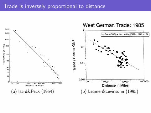
Trade is inversely proportional to distance

(a) Isard&Peck (1954) (b) Leamer&Levinsohn (1995)

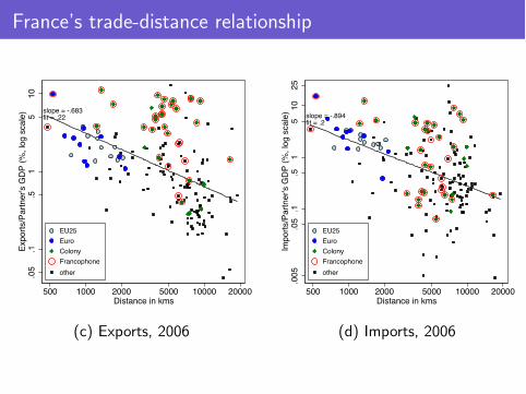
France’s trade-distance relationship

slope = -.683fit = .22

.005

.05

.1.5

15

10Ex

ports

/Par

tner

's G

DP

(%, l

og s

cale

)

500 1000 2000 5000 10000 20000Distance in kms

EU25EuroColonyFrancophoneother

slope = -.894fit = .2

.005

.05

.1.5

15

1025

Impo

rts/P

artn

er's

GD

P (%

, log

sca

le)

500 1000 2000 5000 10000 20000Distance in kms

EU25EuroColonyFrancophoneother

(c) Exports, 2006 (d) Imports, 2006

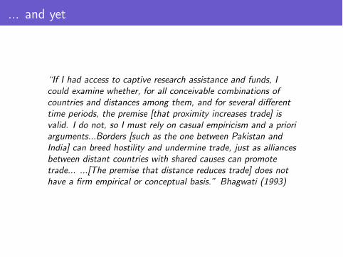
... and yet

“If I had access to captive research assistance and funds, Icould examine whether, for all conceivable combinations ofcountries and distances among them, and for several differenttime periods, the premise [that proximity increases trade] isvalid. I do not, so I must rely on casual empiricism and a prioriarguments...Borders [such as the one between Pakistan andIndia] can breed hostility and undermine trade, just as alliancesbetween distant countries with shared causes can promotetrade... ...[The premise that distance reduces trade] does nothave a firm empirical or conceptual basis.” Bhagwati (1993)

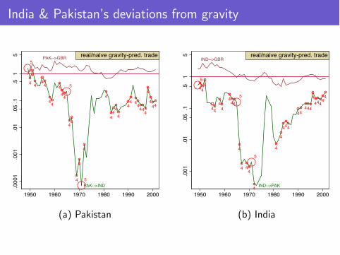
India & Pakistan’s deviations from gravity

PAK-->IND

4

4

44

4

44

4

44

44

4

4

4

4

44

4

4

44 4

444

4

4

444

5

5

5

PAK-->GBR

.00

01

.00

1.0

1.0

5.1

.51

5

1950 1960 1970 1980 1990 2000

real/naive gravity-pred. trade

IND-->PAK

44

4

44

44

444

4

4 44

4

4

4

444

44444

4

4444

4

5

5

5

IND-->GBR

.00

1.0

1.0

5.1

.51

5

1950 1960 1970 1980 1990 2000

real/naive gravity-pred. trade

(a) Pakistan (b) India

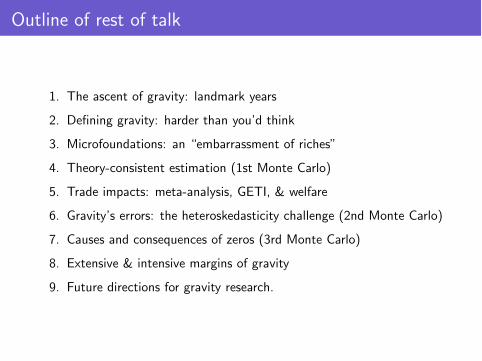
Outline of rest of talk

1. The ascent of gravity: landmark years

2. Defining gravity: harder than you’d think

3. Microfoundations: an “embarrassment of riches”

4. Theory-consistent estimation (1st Monte Carlo)

5. Trade impacts: meta-analysis, GETI, & welfare

6. Gravity’s errors: the heteroskedasticity challenge (2nd Monte Carlo)

7. Causes and consequences of zeros (3rd Monte Carlo)

8. Extensive & intensive margins of gravity

9. Future directions for gravity research.

State of affairs in 1995:

Leamer and Levinshon (1995, HIE): gravity models “have producedsome of the clearest and most robust findings in economics. Butparadoxically they have had no effect on the subject ofinternational economics.”

... “Why don’t trade economists ‘admit’ the effect of distance intotheir thinking?”

One might add: “... still, 40 years after Isard and Peck?”

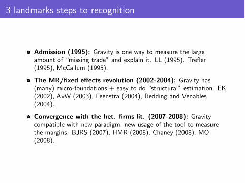
3 landmarks steps to recognition

Admission (1995): Gravity is one way to measure the largeamount of “missing trade” and explain it. LL (1995). Trefler(1995), McCallum (1995).

The MR/fixed effects revolution (2002-2004): Gravity has(many) micro-foundations + easy to do “structural” estimation. EK(2002), AvW (2003), Feenstra (2004), Redding and Venables(2004).

Convergence with the het. firms lit. (2007-2008): Gravitycompatible with new paradigm, new usage of the tool to measurethe margins. BJRS (2007), HMR (2008), Chaney (2008), MO(2008).

Section 1

Microfoundations for Gravity Equations

Defining gravity

3 definitions:

1. General structural gravity

2. Special structural gravity

3. Naive gravity

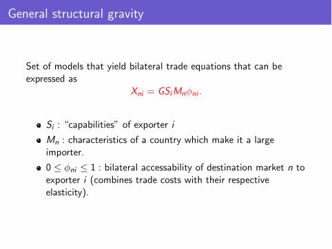
General structural gravity

Set of models that yield bilateral trade equations that can beexpressed as

Xni = GSiMnφni .

Si : “capabilities” of exporter i

Mn : characteristics of a country which make it a largeimporter.

0 ≤ φni ≤ 1 : bilateral accessability of destination market n toexporter i (combines trade costs with their respectiveelasticity).

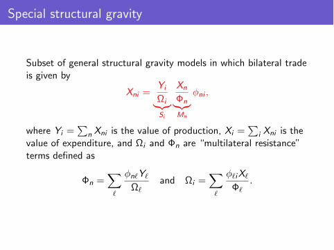
Special structural gravity

Subset of general structural gravity models in which bilateral tradeis given by

Xni =Yi

ΩiSi

Xn

ΦnMn

φni ,

where Yi =

n Xni is the value of production, Xi =

i Xni is thevalue of expenditure, and Ωi and Φn are “multilateral resistance”terms defined as

Φn =

φnY

Ωand Ωi =

φiX

Φ.

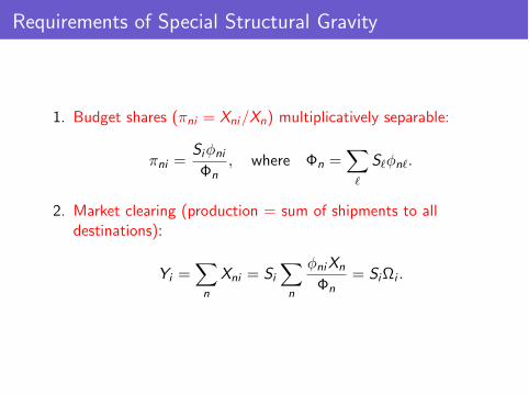
Requirements of Special Structural Gravity

1. Budget shares (πni = Xni/Xn) multiplicatively separable:

πni =Siφni

Φn, where Φn =

Sφn.

2. Market clearing (production = sum of shipments to alldestinations):

Yi =

n

Xni = Si

n

φniXn

Φn= SiΩi .

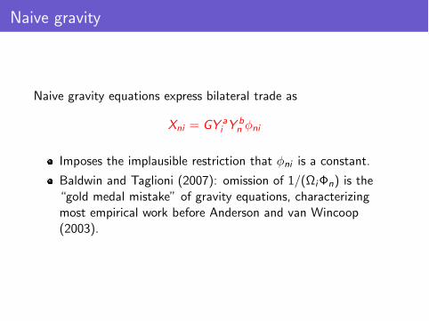
Naive gravity

Naive gravity equations express bilateral trade as

Xni = GY ai Y

bn φni

Imposes the implausible restriction that φni is a constant.

Baldwin and Taglioni (2007): omission of 1/(ΩiΦn) is the“gold medal mistake” of gravity equations, characterizingmost empirical work before Anderson and van Wincoop(2003).

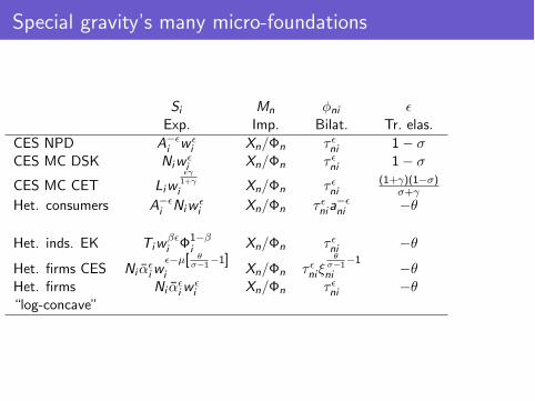
Special gravity’s many micro-foundations

Si Mn φni Exp. Imp. Bilat. Tr. elas.

CES NPD A−i w

i Xn/Φn τ ni 1− σCES MC DSK Niw

i Xn/Φn τ ni 1− σ

CES MC CET Liwγ1+γ

i Xn/Φn τ ni(1+γ)(1−σ)

σ+γ

Het. consumers A−i Niw

i Xn/Φn τ nia−ni −θ

Het. inds. EK Tiwβi Φ1−β

i Xn/Φn τ ni −θ

Het. firms CES Ni αiw

−µ[ θσ−1

−1]i Xn/Φn τ niξ

θσ−1

−1

ni −θHet. firms Ni α

iwi Xn/Φn τ ni −θ

“log-concave”

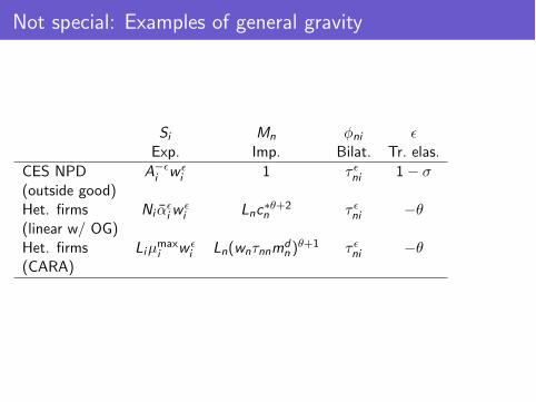
Not special: Examples of general gravity

Si Mn φni Exp. Imp. Bilat. Tr. elas.

CES NPD A−i w

i 1 τ ni 1− σ(outside good)Het. firms Ni α

iwi Lnc∗θ+2

n τ ni −θ(linear w/ OG)Het. firms Liµmax

i w i Ln(wnτnnmd

n )θ+1 τ ni −θ

(CARA)

Gravity for other flows

Human movement: migration, commuting, and tourism.

Anderson (2011, Ann. Rev.) presents a migration gravity modeldrawing on discrete choice techniques. Ahlfeldt et al. (2010) drawon Eaton and Kortum (2002) to specify a commuting gravity model.

Service offshoring. Head et al. (2009) adapt the Eaton andKortum (2002) model to the case of service offshoring.

Cross-border asset ownership. Martin and Rey (2004) propose a2-country model that they use to justify a gravity equation forbilateral portfolio investment. Head and Ries (2008) consider amodel generating a gravity equation for FDI, when it takes the formof acquisitions.

Section 2

Theory-consistent estimation

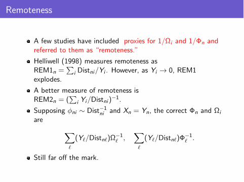
Remoteness

A few studies have included proxies for 1/Ωi and 1/Φn andreferred to them as “remoteness.”

Helliwell (1998) measures remoteness asREM1n =

i Distni/Yi . However, as Yi → 0, REM1

explodes.

A better measure of remoteness isREM2n = (

i Yi/Distni )−1.

Supposing φni ∼ Dist−1

ni and Xn = Yn, the correct Φn and Ωi

are

(Y/Distn)Ω−1

,

(Y/Distn)Φ−1

.

Still far off the mark.

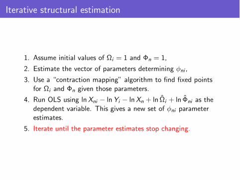
Iterative structural estimation

1. Assume initial values of Ωi = 1 and Φn = 1,

2. Estimate the vector of parameters determining φni ,

3. Use a “contraction mapping” algorithm to find fixed pointsfor Ωi and Φn given those parameters.

4. Run OLS using lnXni − lnYi − lnXn + ln Ωi + ln Φni as thedependent variable. This gives a new set of φni parameterestimates.

5. Iterate until the parameter estimates stop changing.

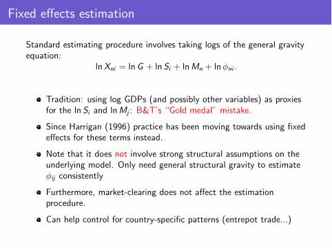
Fixed effects estimation

Standard estimating procedure involves taking logs of the general gravityequation:

lnXni = lnG + ln Si + lnMn + lnφni .

Tradition: using log GDPs (and possibly other variables) as proxiesfor the ln Si and lnMj : B&T’s “Gold medal” mistake.

Since Harrigan (1996) practice has been moving towards using fixedeffects for these terms instead.

Note that it does not involve strong structural assumptions on theunderlying model. Only need general structural gravity to estimateφij consistently

Furthermore, market-clearing does not affect the estimationprocedure.

Can help control for country-specific patterns (entrepot trade...)

Monte Carlo study of different estimators

Monte Carlo using special structural gravity as a DGP.

We use actual data for 170 countries that have GDP,distance, and RTA data in 2006.

φni = exp(− ln Distni + 0.5RTAni )ηni .

2 types of missing values: suppress X% of observationsrandomly, or smallest X% of the initial set of export flows.

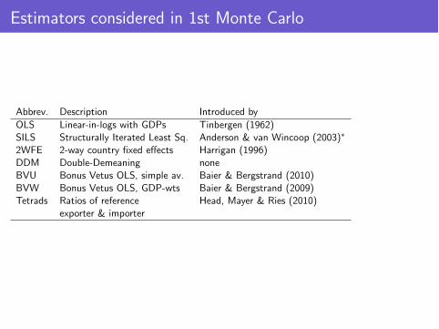
Estimators considered in 1st Monte Carlo

Abbrev. Description Introduced byOLS Linear-in-logs with GDPs Tinbergen (1962)SILS Structurally Iterated Least Sq. Anderson & van Wincoop (2003)∗

2WFE 2-way country fixed effects Harrigan (1996)DDM Double-Demeaning noneBVU Bonus Vetus OLS, simple av. Baier & Bergstrand (2010)BVW Bonus Vetus OLS, GDP-wts Baier & Bergstrand (2009)Tetrads Ratios of reference Head, Mayer & Ries (2010)

exporter & importer

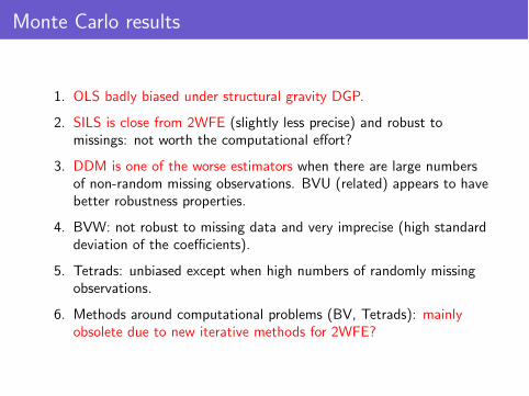
Monte Carlo results

1. OLS badly biased under structural gravity DGP.

2. SILS is close from 2WFE (slightly less precise) and robust tomissings: not worth the computational effort?

3. DDM is one of the worse estimators when there are large numbersof non-random missing observations. BVU (related) appears to havebetter robustness properties.

4. BVW: not robust to missing data and very imprecise (high standarddeviation of the coefficients).

5. Tetrads: unbiased except when high numbers of randomly missingobservations.

6. Methods around computational problems (BV, Tetrads): mainlyobsolete due to new iterative methods for 2WFE?

Section 3

Gravity estimates of policy impacts

Meta-analysis of gravity coefficients

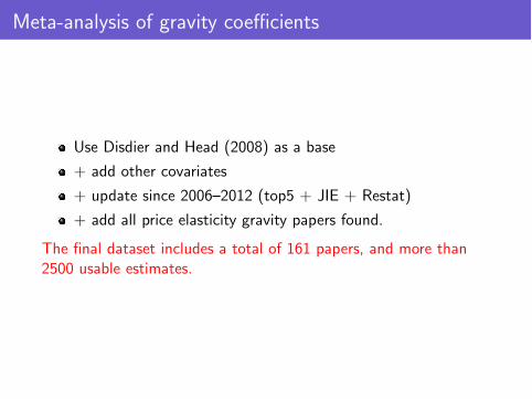
Use Disdier and Head (2008) as a base

+ add other covariates

+ update since 2006–2012 (top5 + JIE + Restat)

+ add all price elasticity gravity papers found.

The final dataset includes a total of 161 papers, and more than2500 usable estimates.

Meta-analysis of gravity coefficients

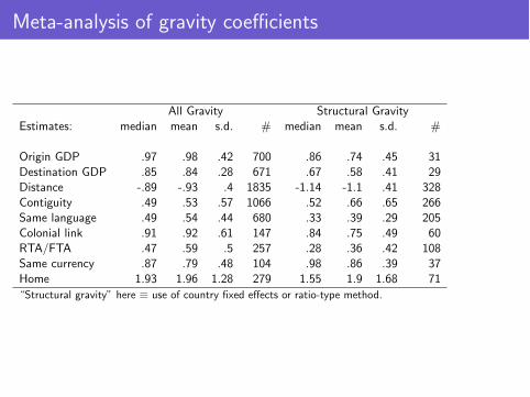
All Gravity Structural GravityEstimates: median mean s.d. # median mean s.d. #

Origin GDP .97 .98 .42 700 .86 .74 .45 31Destination GDP .85 .84 .28 671 .67 .58 .41 29Distance -.89 -.93 .4 1835 -1.14 -1.1 .41 328Contiguity .49 .53 .57 1066 .52 .66 .65 266Same language .49 .54 .44 680 .33 .39 .29 205Colonial link .91 .92 .61 147 .84 .75 .49 60RTA/FTA .47 .59 .5 257 .28 .36 .42 108Same currency .87 .79 .48 104 .98 .86 .39 37Home 1.93 1.96 1.28 279 1.55 1.9 1.68 71“Structural gravity” here ≡ use of country fixed effects or ratio-type method.

Comments on meta-results

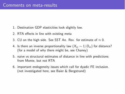
1. Destination GDP elasticities look slightly low.

2. RTA effects in line with existing meta

3. CU on the high side. See SST An. Rev. for estimate of ≈ 0.

4. Is there an inverse proportionality law (Xni ∼ 1/Dni ) for distance?(for a model of why there might be, see Chaney)

5. naive vs structural estimates of distance in line with predictionsfrom Monte, but not RTA

6. important endogeneity issues which call for dyadic FE inclusion.(not investigated here, see Baier & Bergstrand)

Price-shifter elasticities

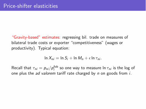
“Gravity-based” estimates: regressing bil. trade on measures ofbilateral trade costs or exporter “competitiveness” (wages orproductivity). Typical equation:

lnXni = ln Si + lnMn + ln τni .

Recall that τni = pni/pfobi so one way to measure ln τni is the log ofone plus the ad valorem tariff rate charged by n on goods from i .

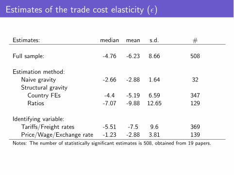
Estimates of the trade cost elasticity ()

Estimates: median mean s.d. #

Full sample: -4.76 -6.23 8.66 508

Estimation method:Naive gravity -2.66 -2.88 1.64 32Structural gravity

Country FEs -4.4 -5.19 6.59 347Ratios -7.07 -9.88 12.65 129

Identifying variable:Tariffs/Freight rates -5.51 -7.5 9.6 369Price/Wage/Exchange rate -1.23 -2.88 3.81 139

Notes: The number of statistically significant estimates is 508, obtained from 19 papers.

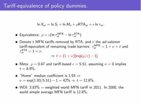
Tariff-equivalence of policy dummies.

lnXni = ln Si + lnMn + ρRTAni + ln τni .

Equivalence: ρ = (ln τMFNni − ln τRTAni )

Denote t MFN tariffs removed by RTA, and ν the ad-valoremtariff-equivalent of remaining trade barriers: τMFN

ni = 1 + ν + t andτRTAni = 1 + ν.

⇒ t = (1 + ν)[exp(ρ/)− 1].

Meta: ρ = 0.47 and tariff-based = 5.51, assuming ν = 0 impliest = 8.9%.

“Home” median coefficient is 1.93 ⇒ν = exp(1.93/5.51)− 1 = 42% ⇒ t = 12.6%.

WDI: 3.83% = weighted world MFN tariff in 2011. In 2000, theworld simple average MFN tariff is 12.8%.

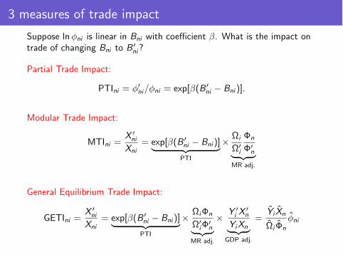
3 measures of trade impact

Suppose lnφni is linear in Bni with coefficient β. What is the impact ontrade of changing Bni to B

ni?

Partial Trade Impact:

PTIni = φni/φni = exp[β(B

ni − Bni )].

Modular Trade Impact:

MTIni =X ni

Xni= exp[β(B

ni − Bni )] PTI

× Ωi

Ωi

Φn

Φn

MR adj.

General Equilibrium Trade Impact:

GETIni =X ni

Xni= exp[β(B

ni − Bni )] PTI

× ΩiΦn

ΩiΦ

n

MR adj.

× Y i X

n

YiXn GDP adj.

=Yi Xn

Ωi Φn

φni

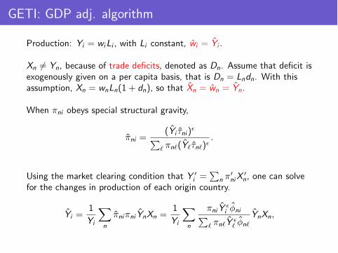
GETI: GDP adj. algorithm

Production: Yi = wiLi , with Li constant, wi = Yi .

Xn = Yn, because of trade deficits, denoted as Dn. Assume that deficit isexogenously given on a per capita basis, that is Dn = Lndn. With thisassumption, Xn = wnLn(1 + dn), so that Xn = wn = Yn.

When πni obeys special structural gravity,

πni =(Yi τni )

πn(Yτn).

Using the market clearing condition that Y i =

n π

niX

n, one can solve

for the changes in production of each origin country.

Yi =1

Yi

n

πniπni YnXn =1

Yi

n

πni Y i φni

πnY φn

YnXn,

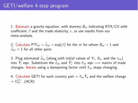
GETI/welfare 4-step program

1. Estimate a gravity equation, with dummy Bni indicating RTA/CU withcoefficient β and the trade elasticity, , or use results from ourmeta-analysis.

2. Calculate PTIni = φni = exp(β) for the ni for whom Bni = 1 andφni = 1 for all other pairs.

3. Plug estimated φni (along with initial values of Yi , Xn, and the πni )into Yi eqn. Substitute the φni and Y

i into πni eqn =⇒ matrix of tradechanges. Iterate using a dampening factor until πni stops changing.

4. Calculate GETI for each country pair = πni Yn and the welfare change= π1/

nn . (ACR)

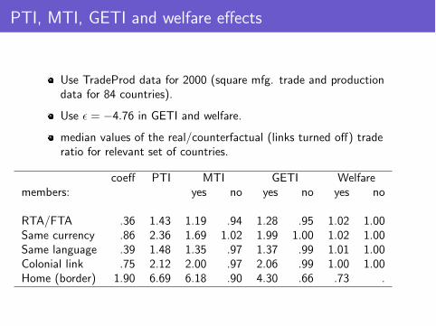
PTI, MTI, GETI and welfare effects

Use TradeProd data for 2000 (square mfg. trade and productiondata for 84 countries).

Use = −4.76 in GETI and welfare.

median values of the real/counterfactual (links turned off) traderatio for relevant set of countries.

coeff PTI MTI GETI Welfaremembers: yes no yes no yes no

RTA/FTA .36 1.43 1.19 .94 1.28 .95 1.02 1.00Same currency .86 2.36 1.69 1.02 1.99 1.00 1.02 1.00Same language .39 1.48 1.35 .97 1.37 .99 1.01 1.00Colonial link .75 2.12 2.00 .97 2.06 .99 1.00 1.00Home (border) 1.90 6.69 6.18 .90 4.30 .66 .73 .

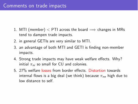
Comments on trade impacts

1. MTI (member) < PTI across the board =⇒ changes in MRstend to dampen trade impacts.

2. in general GETIs are very similar to MTI.

3. an advantage of both MTI and GETI is finding non-memberimpacts.

4. Strong trade impacts may have weak welfare effects. Why?initial πni so small for CU and colonies.

5. 27% welfare losses from border effects. Distortion towardsinternal flows is a big deal (we think) because πnn high due tolow distance to self.

Section 4

Frontiers of gravity research

3 topics w/ “unsettled” questions

1. Gravity’s errors

2. Causes and consequences of zeros

3. Firm-level gravity, extensive and intensive margins

Gravity’s errors

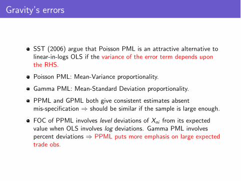
SST (2006) argue that Poisson PML is an attractive alternative tolinear-in-logs OLS if the variance of the error term depends uponthe RHS.

Poisson PML: Mean-Variance proportionality.

Gamma PML: Mean-Standard Deviation proportionality.

PPML and GPML both give consistent estimates absentmis-specification ⇒ should be similar if the sample is large enough.

FOC of PPML involves level deviations of Xni from its expectedvalue when OLS involves log deviations. Gamma PML involvespercent deviations ⇒ PPML puts more emphasis on large expectedtrade obs.

Pseudo ML

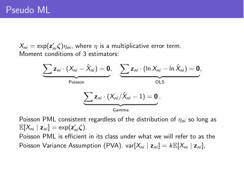
Xni = exp(zniζ)ηni , where η is a multiplicative error term.Moment conditions of 3 estimators:

zni · (Xni − Xni ) = 0

Poisson

,

zni · (lnXni − ln Xni ) = 0

OLS

,

zni · (Xni/Xni − 1) = 0

Gamma

.

Poisson PML consistent regardless of the distribution of ηni so long asE[Xni | zni ] = exp(zniζ).

Poisson PML is efficient in its class under what we will refer to as the

Poisson Variance Assumption (PVA). var[Xni | zni ] = kE[Xni | zni ],

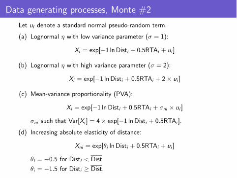
Data generating processes, Monte #2

Let ui denote a standard normal pseudo-random term.

(a) Lognormal η with low variance parameter (σ = 1):

Xi = exp[−1 lnDisti + 0.5RTAi + ui ]

(b) Lognormal η with high variance parameter (σ = 2):

Xi = exp[−1 lnDisti + 0.5RTAi + 2× ui ]

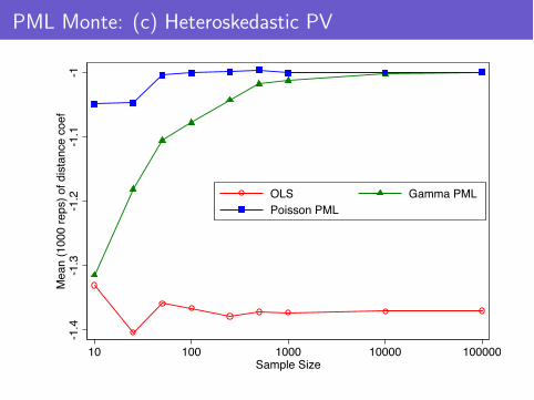
(c) Mean-variance proportionality (PVA):

Xi = exp[−1 lnDisti + 0.5RTAi + σni × ui ]

σni such that Var[Xi ] = 4× exp[−1 lnDisti + 0.5RTAi ].

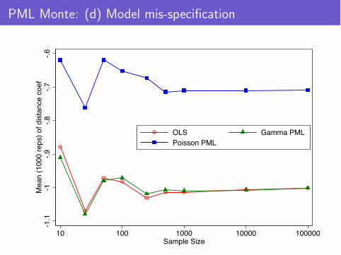
(d) Increasing absolute elasticity of distance:

Xni = exp[θi ln Disti + 0.5RTAi + ui ]

θi = −0.5 for Disti < Dist

θi = −1.5 for Disti ≥ Dist.

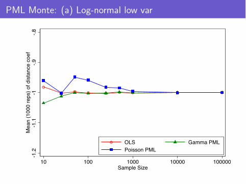
PML Monte: (a) Log-normal low var

-1.2

-1.1

-1-.

9-.

8M

ean (

1000 r

eps)

of dis

tance c

oef

10 100 1000 10000 100000Sample Size

OLS Gamma PML

Poisson PML

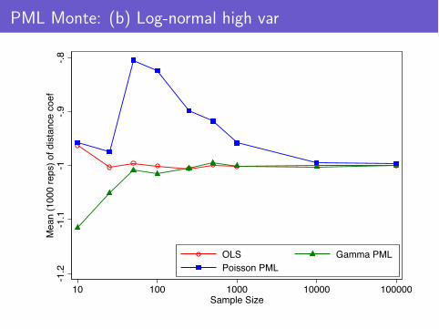
PML Monte: (b) Log-normal high var

-1.2

-1.1

-1-.

9-.

8M

ean (

1000 r

eps)

of dis

tance c

oef

10 100 1000 10000 100000Sample Size

OLS Gamma PML

Poisson PML

PML Monte: (c) Heteroskedastic PV

-1.4

-1.3

-1.2

-1.1

-1M

ean (

1000 r

eps)

of dis

tance c

oef

10 100 1000 10000 100000Sample Size

OLS Gamma PML

Poisson PML

PML Monte: (d) Model mis-specification

-1.1

-1-.

9-.

8-.

7-.

6M

ean (

1000 r

eps)

of dis

tance c

oef

10 100 1000 10000 100000Sample Size

OLS Gamma PML

Poisson PML

Gravity’s errors: cookbook

We recommend all 3 models should be estimated.

1. If 3 estimates are similar, model seems well-specified, error lognormal with a constant variance: Relax.

2. If PPML and GPML are similar and distinct from OLS,heteroskedasticity is probably a problem: OLS unreliable.

3. If Gamma and OLS are similar and Poisson coeffs are smaller inabsolute magnitude (a case we have seen in practice):

(a) RMSE large + small sample: possible small sample bias ofeither the Poisson PML or the Gamma PML.

(b) Large sample: trade costs may have a non-constant elasticity.Major divergence between Poisson and Gamma PML in largesamples is a sign of model mis-specification.

Causes and consequences of zeros

Multiplicative models, in which expected bilateral trade isgiven by E[Xni | zni ] = exp(zniζ), do not naturally generatezero flows.

Actual trade can exhibit substantial fractions of zeros,

Zeros become more frequent with disaggregation at the firmor product level.

Even at the country level, not all small countries tradepositive amounts with other small countries.

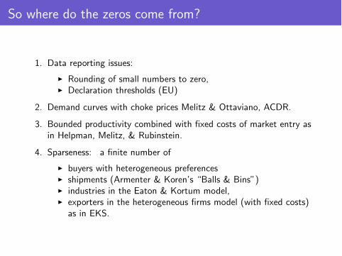
So where do the zeros come from?

1. Data reporting issues:

Rounding of small numbers to zero, Declaration thresholds (EU)

2. Demand curves with choke prices Melitz & Ottaviano, ACDR.

3. Bounded productivity combined with fixed costs of market entry asin Helpman, Melitz, & Rubinstein.

4. Sparseness: a finite number of

buyers with heterogeneous preferences shipments (Armenter & Koren’s “Balls & Bins”) industries in the Eaton & Kortum model, exporters in the heterogeneous firms model (with fixed costs)

as in EKS.

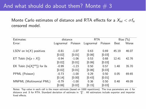
And what should do about them? Monte # 3

Monte Carlo estimates of distance and RTA effects for a Xni < σfncensored model.

Estimates: distance RTA Bias (%)Error: Lognormal Poisson Lognormal Poisson Best Worse

LSDV on ln(X ) positives -0.81 -1.07 0.63 0.69 45.19 46.07[0.02] [0.01] [0.06] [0.03]

ET Tobit (ln[a+ X ]) -0.94 -1.06 0.53 0.68 12.41 42.76[0.02] [0.01] [0.06] [0.03]

EK Tobit (ln[Xminn ]) for 0s -0.99 -1.23 0.50 0.57 1.48 35.70

[0.02] [0.01] [0.06] [0.03]PPML (Poisson) -0.73 -1.00 0.29 0.50 0.05 69.65

[0.14] [0.00] [0.43] [0.01]MNPML (Multinomial PML) -0.79 -1.00 0.36 0.50 0.48 49.09

[0.06] [0.02] [0.15] [0.03]Notes: Top value in each cell is the mean estimate (based on 1000 repetitions). The true parameters are -1 fordistance and .5 for RTA. Standard deviation of estimate in “[]”. All estimators include exporter and importerfixed effects.

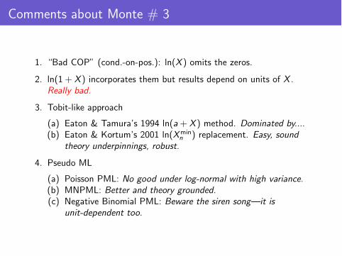
Comments about Monte # 3

1. “Bad COP” (cond.-on-pos.): ln(X ) omits the zeros.

2. ln(1 + X ) incorporates them but results depend on units of X .Really bad.

3. Tobit-like approach

(a) Eaton & Tamura’s 1994 ln(a+ X ) method. Dominated by....(b) Eaton & Kortum’s 2001 ln(Xmin

n ) replacement. Easy, soundtheory underpinnings, robust.

4. Pseudo ML

(a) Poisson PML: No good under log-normal with high variance.(b) MNPML: Better and theory grounded.(c) Negative Binomial PML: Beware the siren song—it is

unit-dependent too.

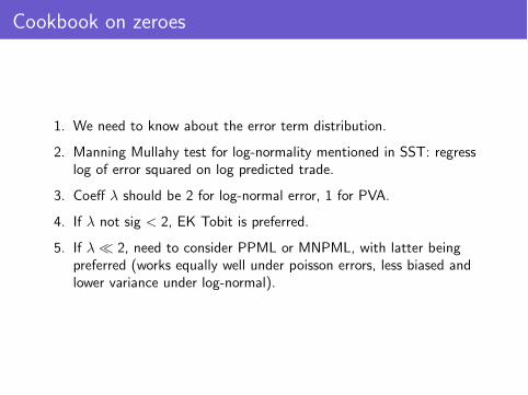
Cookbook on zeroes

1. We need to know about the error term distribution.

2. Manning Mullahy test for log-normality mentioned in SST: regresslog of error squared on log predicted trade.

3. Coeff λ should be 2 for log-normal error, 1 for PVA.

4. If λ not sig < 2, EK Tobit is preferred.

5. If λ 2, need to consider PPML or MNPML, with latter beingpreferred (works equally well under poisson errors, less biased andlower variance under log-normal).

Extensive and intensive margins

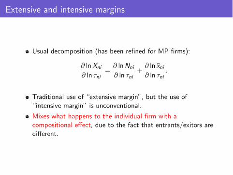
Usual decomposition (has been refined for MP firms):

∂ lnXni

∂ ln τni=

∂ lnNni

∂ ln τni+

∂ ln xni∂ ln τni

.

Traditional use of “extensive margin”, but the use of“intensive margin” is unconventional.

Mixes what happens to the individual firm with acompositional effect, due to the fact that entrants/exitors aredifferent.

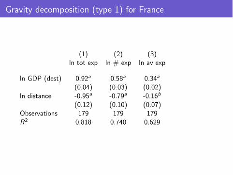
Gravity decomposition (type 1) for France

(1) (2) (3)ln tot exp ln # exp ln av exp

ln GDP (dest) 0.92a 0.58a 0.34a

(0.04) (0.03) (0.02)ln distance -0.95a -0.79a -0.16b

(0.12) (0.10) (0.07)Observations 179 179 179R2 0.818 0.740 0.629

3 Margins

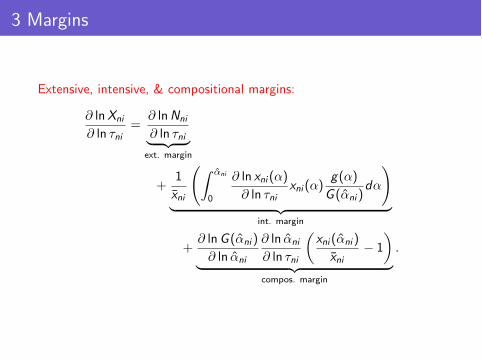
Extensive, intensive, & compositional margins:

∂ lnXni

∂ ln τni=

∂ lnNni

∂ ln τni ext. margin

+1

xni

αni

0

∂ ln xni (α)

∂ ln τnixni (α)

g(α)

G (αni )dα

int. margin

+∂ lnG (αni )

∂ ln αni

∂ ln αni

∂ ln τni

xni (αni )

xni− 1

compos. margin

.

Advantages of 3 margins

Nests existing 2-way decompositions: BJRS/MO (type 1) andChaney (type 2)

Intensive and extensive are “empirically measurable”1. Extensive is elasticity of # of exporters2. Intensive is elasticity of average exports of the “constant

sample” of firms.3. Compositional is a residual

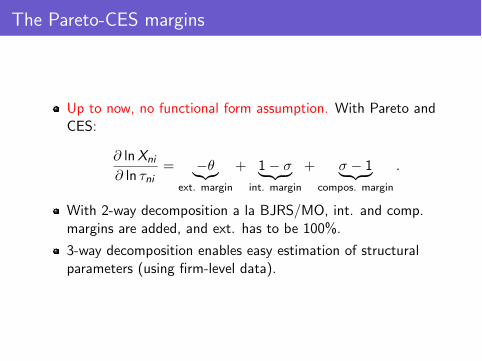
The Pareto-CES margins

Up to now, no functional form assumption. With Pareto andCES:

∂ lnXni

∂ ln τni= −θ

ext. margin

+ 1− σ int. margin

+ σ − 1 compos. margin

.

With 2-way decomposition a la BJRS/MO, int. and comp.margins are added, and ext. has to be 100%.

3-way decomposition enables easy estimation of structuralparameters (using firm-level data).

Future directions for gravity research

1. Digging deeper: Why do the things that matter (distance,language, borders, currencies?) matter as much as they do,even now?

2. Restrictive functional form assumptions: how big of aproblem?

3. Dynamics of gravity

Concluding thoughts

Gravity is an interesting example of1. Strong empirical evidence pushing theory to think about

micro-foundations.2. Theoretical progress changing radically the way those

equations are estimated.

We provide an integrated framework to organise the vastnumbers of micro-foundations

We use quantitative methods to provide cookbook-stylerecommendations about which estimation methods to use andhow to interpret results, notably for policy relevant variables.

Our selective survey of topics at the frontier of currentresearch suggests that a great deal of interesting work liesahead.