Green Electricity Investments: Environmental Target

and the Optimal Subsidy∗

Simona Bigerna1, Xingang Wen†2, Verena Hagspiel3, and Peter M. Kort4,5

1Department of Economics, University of Perugia, 06123 Perugia, Italy2Department of Business Administration and Economics, University of Bielefeld, 33501 Bielefeld, Germany

3Department of Industrial Economics and Technology Management, Norwegian University of Science and

Technology, 7491 Trondheim, Norway4Department of Econometrics and Operations Research & CentER, Tilburg University, LE 5000 Tilburg, The

Netherlands5Department of Economics, University of Antwerp, 2000 Antwerp, Belgium

Abstract

We investigate the optimal investment decision in renewables under market demand uncer-

tainty, in the context of the Italian strategy for renewable deployment under the EU policy.

Upon investing, the firm has to decide about the time and size of the investment. We find that

a higher subsidy level induces the firm to invest earlier with a smaller investment capacity. This

implies that a given environmental target cannot be reached by a too high (too low) subsidy

level since this will cause the investment level to be low (too late). We show that there exists

an optimal (intermediate) subsidy level to reach the environmental target. Furthermore we find

that in a more uncertain economic environment the subsidy adjustment to maintain the target

level of investment results in the firm investing earlier, which is opposite to the standard real

options result.

Keywords: Investment under uncertainty, Renewable energy sources, Public subsidies, Invest-

ment timing, Investment size

JEL subject classification: D81, L51∗Xingang Wen gratefully acknowledges support from the German Research Foundation (DFG) via CRC 1283, and

Peter M. Kort thanks Engie for financial support Grant “FFP160134”.†Corresponding author: Tel.: +49 521 106 3942. Email: xingang.wen@uni-bielefeld.de

1

1 Introduction

Deployment of renewable energy source (RES) is a primary concern of the EU 2020 policy, which

has been geared to set subsidy levels capable to spur new investment. A recent new target of the

European Union (EU) Commission, according to “2030 framework for climate and energy policies”,

is to achieve 27% of RES in total energy consumption for the entire EU, without detailing individual

targets for member countries. At the same time, the EU commission suggests to adopt a feed-in-

premium (FIP) and abandon the fixed feed-in-tariff (FIT) instrument, on the ground that more

market approach is apt and some risk should be shared between investor and consumers (European

Commission, 2014).

The EU policy framework envisions the achievement of a desired RES target with subsidies, and

to close the gap between the market price of conventionally sourced energy and the opportunity cost

of new RES. In many member countries, the subsidy has been typically implemented as a fixed FIT

to provide a clear and certain support to RES policy (European Commission, 2017). However, firms

do not necessarily invest more in RES when the subsidy increases (International Energy Agency,

2015). They may react by a lower than expected investment level, if uncertainty characterizes the

perception of future market demand. Furthermore, the firm can change the investment time, which

can have its own implication for the size of the investment. Therefore, in order to study the policy

effectiveness, there is a need to model the firms’ decision to account for dynamic uncertainty that

impacts the RES investment profitability. In a market with uncertain future demand, the firm is

constantly forecasting demand and balancing the value of investing now and delaying investments.

For these features, we employ a real options approach to analyze the investment decisions, where we

do not only focus on timing as in the traditional real option analysis (see, e.g., Dixit and Pindyck

(1994)), but also on the investment size.

This paper sets up and empirically tests a general model to analyze the investment decision

in RES using the real option approach under dynamic uncertainty. We model three stochastic

components that affect the firm’s profitability, namely, demand fluctuations, changes in consumer

attitude toward environmental issues, and cost decrease due to innovation and decreasing learning

curves. We contribute to the literature in three ways. First, we provide a theoretical model for

the firm’s decision to invest in RES. Secondly, we calibrate the model with Italian data and study

the impact of the government subsidy policy in Italy. Thirdly, we propose an intermediate level of

subsidy support to achieve the desired target of the new EU policy.

2

We show that to reach the target it is not just a matter of setting a high enough subsidy level.

This is because the firm reacts to an increased subsidy by investing earlier and less. What the

government needs to do is to determine a subsidy level such that the firm invests just enough to

reach the target. Hence, the investment is as low as possible in light of the target, which implies

that then the firm invests as early as possible with respect to reaching the target in time. In a

changing economic environment the subsidy level needs to be adjusted such that the target is still

reached. This has the implication that, surprisingly, the firm is expected to invest earlier in a

more uncertain environment. The reason is that the direct effect, implying the usual result that

the firm invests later when there is more uncertainty, is more than counterbalanced by an indirect

effect. This indirect effect is caused by the fact that an increased subsidy level is needed to keep

on reaching the target when uncertainty goes up, and this increased subsidy causes a substantial

acceleration of investment. If the environmental target cannot be reached, a conditional subsidy

rule may help: Only when the demand level is high enough, the subsidy will be issued from that

moment on. This is to prevent that the firm invests in a too low capacity level.

This paper is organized as follows. Section 2 reviews the relevant literature of real options

modelling of the firm’s RES investment decision. Section 3 sets up the theoretical model and derives

the firm’s optimal investment decision under subsidy support. Section 4 shows the calibration of

the model for Italy, using the policy targets for 2020 and a scenario target for 2035, and analyzes

the firm’s investment decision in light of the target and the corresponding subsidy level. Section

5 discusses the results of some sensitivity analysis of the model parameters. Section 6 shows the

conclusions and policy implications.

2 Related Literature

The real options approach proves that investment irreversibility and an uncertain economic envi-

ronment create a value of waiting with investment. The firm postpones its investment in order to

wait for more information about future uncertainty. Applying a real options approach to analyze

the firm’s investment took off with Dixit and Pindyck (1994). This research mainly determines

the timing of the investment. Dangl (1999) is among the first to include the decision of optimal

investment size. Recently, more contributions acknowledge that investing is not only about timing

but also about determining the optimal size, see e.g., Huisman and Kort (2015); Hagspiel et al.

(2016a) and Hagspiel et al. (2016b). A main result of this literature is that increased uncertainty

3

not only delays the time of the investment but also increases its size.

The real options approach has been widely used to analyze the firm’s investment decision in re-

newable energy projects under uncertainty while taking into account different policy instruments.

It is a suitable descriptor of the observed investment behavior compared to the net present value

rule (Fleten et al., 2016) and has been used to analyze regulatory uncertainty impact on invest-

ment decisions (Pawlina and Kort, 2005; Boomsma et al., 2012; Boomsma and Linnerud, 2015;

Chronopoulos et al., 2016). Some literature focuses on policy measures like subsidies. This is be-

cause energy production from green technologies is usually more costly, and only public subsidies

can make the market entry attractive to investors (Nesta et al., 2014). For instance, Ritzenhofen

and Spinler (2016) conclude that a fixed subsidy level leads to an immediate decision to invest now

or never, and Boomsma et al. (2012) show that FIT encourages earlier investment. Some other

contributions emphasize on different policy instruments such as a price cap, and their influence on

private firms’ investments to achieve the first-best outcome. This stream of literature is represented

by Evans and Guthrie (2012), Broer and Zwart (2013), Gatzert and Vogl (2016), and Willems and

Zwart (2017).

Several research papers have looked into the influence of policy instruments from an empirical

perspective. Fleten et al. (2007) consider the problem of investing in a generator. In a case

study, Fleten et al. (2007) focus on the situation at the Nord pool, and show that it is worthwhile

to wait for higher prices under price uncertainty. Boomsma et al. (2012) also study the Nordic

case and argue that upon investment, renewable energy certificate trading creates incentives for

larger projects. Zhang et al. (2016) investigate the dynamics of investment value and the optimal

timing for renewable energy investment in China. They find that a subsidy increase would stimulate

investment. Detert and Kotani (2013) analyze the switch option from coal to renewables in Mongolia

under coal price uncertainty. They assume negative externalities from coal-based operations, and

suggest the government should increase electricity prices or switch to renewable energy earlier to

reduce the welfare loss, when people are willing to pay more to remove the negative externalities.

However, to the best of our knowledge, there is little research on how to reach the RES deployment

target by optimally determining the policy instrument level. This paper intends to fill the void and

presents a theoretical analysis of the public policy with an empirical application to the Italian RES

deployment target.

Several features characterize the RES in Italy. In order to attain 26.4% of green electricity

production from RES by 2020, the government policy has promoted subsidies through a feed-in

4

tariff mechanism for investors. The burden of the subsidy is paid by all consumers with a surcharge

on the electricity bill (Bigerna et al., 2015). The Italian consumer’s willingness to pay for RES is

higher than before. This is because of the positive consumer attitudes towards RES, such as the

willingness to pay as a result of increasing environmental awareness (Bigerna and Polinori, 2014).

In Section 3, a theoretical model is set up that includes such characteristics.

3 Model

3.1 Model Setup

The unit price of green electricity payments, P, which is measured in euro/MWh (or euro/MW),

satisfies a linear inverse demand function with premium s, reflecting the “willingness to pay for

green energy”, i.e.

Pt = γt + st − ηK.

In this formulation η is a positive constant, whereas K stands for green electricity capacity. We

impose that the firm always produces up to capacity.

The time function γt is stochastic to cover unexpected demand fluctuations. It is expected to

increase over time to capture the expected increase of demand for renewable energy over time. The

latter is due to the expected price increase of fossil fuels.

The premium st is subject to uncertainty, because, as argued by Bigerna and Polinori (2014),

uncertainty plays a crucial role in the willingness to pay (WTP) for renewable energy. The WTP,

and thus st, is expected to increase over time, because as time passes consumers get more aware of

environmental problems.

We define ct to be the unit costs for the green energy firm. Due to innovation and a decreasing

learning curve, these costs are expected to decrease over time. Since the future development of

innovation is hard to predict, the development of ct over time will be stochastic, but with decreasing

trend.

Summarizing the above, we can define

Xt = γt + st − ct,

as the sum of the stochastic components, which affect the firm’s profitability. The renewable

energy price for the producer is augmented by a fixed feed-in-premium SF . With this instrument

the government can positively influence renewable energy output. Combining the above expression

5

with the inverse demand function, we can define the net price pt received by the firm as the difference

between the unit price Pt augmented by the feed in premium SF and the unit costs, ct:

pt = Pt + SF − ct = SF +Xt − ηK.

To cover the fact that both γt and st are expected to increase over time, that ct is expected to

decrease over time, and that all are subject to uncertainty, we impose that Xt is a stochastic process

satisfying a geometric Brownian motion process, i.e.

dX = αXdt+ σXdz,

with α and σ being positive constants, whereas dz is the increment of a Wiener process.

Investment costs equal θI, where I is the acquired capacity measured in MW, and θ is a positive

constant. The production function that converts capacity into electricity is linear and given by

K = hI,

where K is the MWh produced and h is the specific productivity coefficient (number of hours).

The value of h takes into account that a solar park has a lower capacity utilization in one year

(1200 hours on average), a wind plant can go up to 4000 hours, and a biomass plant to 6000 hours.

This linear relationship makes that for the investment costs we can write

θI = δK with δ = θ

h.

Given that the firm discounts with rate r, the value the representative firm obtains when under-

taking an investment in capacity K equals

V (X) = maxK

E

∞∫0

e−rtK (Xt + SF − ηK) dt− δK | X0 = X

.The green electricity firm thus faces an investment problem where it has to find the optimal time

and the optimal size of investment. The optimal time is in fact the point in time that the stochastic

process Xt hits the threshold level X∗, provided X0 < X∗. Otherwise, it is optimal for the firm to

invest immediately.

3.2 Optimal Investment Decision

The optimal investment decision can be found in two steps. First, for a given level of the geometric

Brownian motion, denoted by X, the corresponding optimal capacity level of K is found by solving

maxK

E

∞∫0

e−rtK (SF − ηK +Xt) dt− δK | X0 = X

6

= maxK

(K (SF − ηK)

r+ KX

r − α− δK

).

This gives

K = 12η

(SF + r

r − αX − rδ

). (1)

We conclude that the optimal capacity level is increasing in X. Furthermore, at a higher premium

level it is optimal for the firm to invest in a larger capacity so that the total profit flow increases.

Inserting (1) in the profit flow K (SF − ηK +Xt) learns that the profit flow becomes quadratic

in X. Define Y = X2. Then Ito’s lemma gives

dY =(2α+ σ2

)X2dt+ 2σX2dz.

Hence X2 is a geometric Brownian motion process with trend 2α + σ2. This implies that for the

problem to converge we need to impose

r > 2α+ σ2. (2)

Second, we have to derive the optimal investment timing, reflected by the threshold level X∗,

so that the firm stops waiting and invests with capacity K(X∗) at the moment X∗ is reached.

Standard real options analysis (e.g., Dixit and Pindyck (1994)) learns that the value of the option

to invest, denoted by F, is equal to

F (X) = AXβ,

where A is a positive constant and β is the positive root of the quadratic polynomial

12σ

2β2 +(α− 1

2σ2)β − r = 0, (3)

so that

β = 12 −

α

σ2 +

√(12 −

α

σ2

)2+ 2rσ2 > 2. (4)

The inequality follows from the fact that (3) implies that the positive root equals β = 2 for

r = 2α + σ2. However, due to (2) we know that r is larger. This implies that β > 2, since we

conclude from (4) that β is increasing in r.

To determine the threshold level X∗, we employ the value matching and smooth pasting condi-

tions

F (X∗) = V (X∗,K) ,∂F (X)∂X

|X=X∗ = ∂V (X,K)∂X

|X=X∗ .

7

This gives

X∗ = β

β − 1r − αr

(rδ − (SF − ηK)) . (5)

Combining and solving (1) and (5) leads to the following proposition.

Proposition 1 The optimal investment threshold X∗ and the corresponding optimal capacity level

K∗ are given by

X∗ = β

β − 2r − αr

(rδ − SF ) , (6)

K∗ = K (X∗) = rδ − SFη (β − 2) . (7)

3.3 Evaluation

We could confront the resulting investment decision with the fact that, according to some envi-

ronmental treaty, the investment should take place before a certain time and should be sufficiently

large. For instance, “The goal of Italy is to attain 26.4% green electricity (GE) production from

renewable energy sources (RES) by 2020”, where the 26.4% is the share in the total annual produc-

tion of electricity (in MWh). Other big European countries, like Germany and Spain, have similar

objectives that can be analyzed as well.

In this sense it is important to note that the effect of the fixed feed-in premium SF is tricky: on

the one hand we obtain from (6) that it accelerates investment, but on the other hand we get that,

according to (7), the firm invests in less capacity. The latter seems counterintuitive, since X∗ and

thus the output price at the moment of investment is lower, but is caused by the fact that earlier

investment by the firm implies lower profits per unit capacity at the moment of investment, so that

the firm will reduce the investment size. Note that by considering (1) we can conclude that, in case

timing is fixed, capacity goes up with SF .

To reach a specific environmental target like “26.4% green electricity (GE) production in 2020”,

the government first determines the required capacity level K∗. Then by equation (7) we obtain

the corresponding premium level SF , which gives, via (6), the threshold level X∗. In case the firm

is expected to invest too late, we adjust SF to influence the investment decision such that the goal

of this 26.4% in 2020 will be reached. Here a conditional subsidy policy may help: Only when X

has reached a high enough value, the firm can receive the subsidy. This is to prevent that the firm

invests too early in a too low capacity level.

8

4 Derivation of the Optimal Subsidy Level

We take Italy as an example by data from AEEG (2016) and conduct an empirical analysis to

study the renewable subsidy policy. Because Italy has been performing well and realized the 2020

RES target assigned by the EU earlier in 2015, it is easier to calibrate the parameter values from

the historical data. Given the EU policy, we can predict the RES target for Italy. According to the

calibrated parameter values and the analytical results of the theoretical model, we can calculate

the optimal subsidy level to achieve this target.

4.1 Data

In Italy, the total electricity consumption in 2010 was 320 TWh and decreased to 311 TWh in 2015

due to the sluggish economy. In the same period, RES increased from 23% (71 TWh) to about

35% (109 TWh). This means Italy had already reached the 2020 target of 35% by the EU in 2015.

This achievement is largely due to the generous Italian RES policy stance (AEEG, 2016). Note

that the 2020 target for total energy consumption assigned to Italy is 17%, which is smaller than

35% because it includes heating and transportation etc.. In terms of electricity, the target is 35%

of RES.

For the period of 2016-2035, we use the Italian transmission system operator (TSO) forecast of

0.3% annual growth rate for electricity consumption. This results in about 315.7 TWh in 2020

and 330.2 TWh in 2035. We assume that the target of RES in 2020 remains unchanged at 35%.

Therefore, the targeted RES total value in 2020 is about 110.4 TWh. For the time beyond 2020, we

take into account that the European Commission (2014) has formulated a new challenging target

of RES share in 2030, with about 27% of total energy consumption for the EU. We assume this

percentage target remains the same in 2035. Then for Italy, 27% of total energy consumption

implies a RES share of 51% in total electricity consumption. This suggests a RES target value

of 168.4 TWh in 2035. Obviously, this value is under the assumption that the RES policy target

is unchanged and run under the business as usual (BAU) behavior (International Energy Agency,

2016). Nonetheless, as this new EU target is still under discussion, we provide a simulation scenario,

which is useful for the policy formulation.

9

4.2 Calibration

In order to simulate the model, we calibrate the relevant parameters for Italy, using historical data

for the most recent period 2010-2015. We have fitted the demand function to recover the values

for parameters η, γ, and s. We have calibrated the unit cost component c using the computation

of the levelized cost of electricity from Elshurafa et al. (2017). The resulting calibration values

for the initial year 2010 are reported in Table 1. As initial values in the year 2010:1 we fixed:

γ0 + s0 = 185.7; c0 = 175.7; X0 = γ0 + s0 − c0 = 11.4. In this preliminary calibration context, we

assume that the parameters α, r, σ, δ are in a plausible range.

[Table 1]

The simulation of the theoretical model is performed for two separate periods. First, we simulate

the 2010-2015 period to check the validity of the model and whether the model can simulate the

generous Italian subsidy support, which has facilitated to reach the EU 2020 target already in 2015.

Second, we conduct a simulation until the year 2035 to investigate the possible policy framework

to reach the 2035 target.

For both periods, we simulate the geometric Brownian motion according to

Xt = X0 exp((

α− σ2

2

)t+ σWt

),

with 100 random drawings of the Wiener process dWt ∼ N(0, 1). We compute the average of these

100 simulations and check the attainability of the target RES.

4.3 Historical Simulation

We first simulate for the historical period 2010-2015. We have constructed two scenarios with

different levels of SF , labeled A (high subsidy) and C (low subsidy). In Scenario A we set SF = 101

and in Scenario C we set SF = 99. The purpose of these simulations is to check the validity of the

calibrated parameter values and to check the effectiveness of the subsidy policy implemented during

this period. For the given parameter values and the capacity target of 2015, K∗ = 109 TWh, the

optimal subsidy rate to reach this target is equal to SF = 101. Thus, in Scenario A the subsidy

policy is more suitable to reach the target than in Scenario C. We show detailed simulation results

of these scenarios for the investment timing in period 2010-2015, which are reported in Figure 1

and analyzed in Figure 2.

[Figures 1 and Figure 2]

10

For the convenience of graphic illustration, only 10 out of 100 simulated evolution paths of Xt

are demonstrated in Figure 1. Comparing the optimal investment threshold in 1a and 1b, we notice

that X∗ is larger in Scenario C, implying a larger optimal threshold for a lower subsidy rate. This

is coherent with our theoretical results in equation (6), where X∗ decreases with SF . Figure 2

shows for each period the empirical percentage of realizations that reach the optimal threshold.

The high subsidy scenario (A) allows to reach the target in about 20% of the cases already in the

year 2011. This percentage is steadily increasing until 100% of success in 2015. In the low subsidy

scenario (C), the percentage of success in reaching the target remains below 20% up until the year

2015. As these values are close to the historical values, we can conclude that Scenario A represents

the subsidy policy in Italy well and that the subsidy level SF = 101 is close to the historical level.

Thus, the model can explain the boom of RES investment in 2015 that reaches the EU 2020 target.

4.4 Optimal Subsidy Policy to 2035

We now turn to the simulation of the subsidy policy in the period 2016-2035. According to Propo-

sition 1, for the given parameter values in Table 1 and K∗2035 = 168.4 TWh, which is the investment

level needed to reach the environmental target in 2035, we obtain SF2035 = 98.9 and X∗2035 = 19.86.

Given that X0 = 11.4 in 2010, this implies that it would take 23.3 years from 2010 on to realize

the optimal investment size 168.4TWh. In other words, the required capacity K∗ is expected to

be acquired in April 2033. In the following analysis, we check by simulation what happens if the

subsidy rate deviates from the optimal subsidy level SF2035.

[Figure 3]

Figure 3 reports five scenarios for different values of SF and the corresponding fractions of

empirical realization that hit the target value of X∗ in each period until 2035. For instance, for

the subsidy rate SF = 97, scenario E in the figure, the corresponding investment threshold is

X∗(SF = 97) = 25.6, and K∗(SF = 97) = 216.8 TWh. From the simulation, we get that only 8%

of the evolvement paths for Xt can reach 25.6 by 2035, implying that the 2035 target is reached

with 8% probability. A higher level of SF = 101, scenario D in the figure, makes the firm invest

at X∗(SF = 101) = 12.8 with capacity K∗(SF = 101) = 108.4 TWh. This implies that the

environmental target will never be reached because it requires an investment level of 168.4 TWh.

These two scenarios support the theoretical implication of the model: a larger SF makes the firm

invest earlier and less. A small threshold X∗ means it is more likely for Xt to reach X∗ and to

realize the corresponding K∗, but this K∗ can be too low to reach the required investment level.

11

If SF is too low, K∗ is large enough to reach the target, but it is less likely that the geometric

Brownian motion process Xt reaches X∗ before the year 2035. So the investment is expected to

take place too late.

Figure 3 also shows scenarios for SF = 98.9 (B), SF = 100 (C), and SF = 103 (E). Moreover, it

demonstrates the increase of the percentage realization for the corresponding X∗F in period 2016-

2035. For instance, the grey line DDC in Figure 3 illustrates the fraction of realizations where the

threshold target is reached in time in Scenario C. This fraction increases from zero at the beginning

to around 40% in 2016 and over 50% in 2035.

5 Comparative Static Analysis

5.1 Keeping the Policy Instrument SF Fixed

Changes in the market conditions can result in variations of the parameters, and thus influence the

firm’s investment decision. We have conducted a sensitivity analysis around the calibrated values

of the parameters σ, α, δ, and r, to assess the response of the probability of realization of the

target. The results are illustrated in Figure 4 for five different values of each parameter, which are

increasing from Scenario A to Scenario E. In each panel of Figure 4 we show the corresponding

fractions of realizations that hit the target value of X∗ before 2035. We observe that the realization

fraction is decreasing with an increase in each parameter.

[Figure 4]

Panel 4a shows that a smaller σ corresponds to a higher probability of realization, demonstrated

by DDA, implying a lower threshold level X∗. For a given subsidy rate SF , in line with the standard

real options results, an increase in the uncertainty makes the firm undertake a larger investment

and invest later. The intuition is that when there is more uncertainty about the future market, the

firm would like to wait for more information and invest more, because at the moment of investment

market demand is higher.

In panel 4b, as α increases, the probability of the RES target realization decreases. The intuition

is as follows: a larger α implies that the market grows faster, and the firm anticipates a larger future

market demand when deciding on the size of investment. This leads to a larger investment capacity

K∗ and thus more investment costs. So the firm prefers to invest later when market demand is

higher in order to defray the investment costs. This implies that X∗ increases with α. In our

simulations, therefore a negative correlation between α and the fraction of the cases in which the

12

target is reached, prevails.

Panel 4c shows that a larger δ implies a larger X∗ and thus a smaller probability of target

realization, illustrated by DDE, implying a larger X∗. This is because for a given subsidy rate SF ,

a larger δ means investing is more expensive, which motivates the firm to invest later when the

market demand is higher. As for parameter r, note that for the given parameter values, we obtain

that the optimal investment capacity K∗ increases with r, which leads to a larger threshold X∗

and a lower probability of realization of the target as demonstrated by Panel 4d.

5.2 Optimally Adjusting the Policy Instrument SF

With the subsidy instrument, government can anticipate the changing environment and act proac-

tively by adjusting the level of the feed-in premium SF . It does so with the aim to keep the

probability of realizing the target as high as possible. For the corresponding changes in parame-

ters, say σ for instance, in order to guarantee a certain level of investment, the government needs

to adjust SF such that

dK∗

dσ = ∂K∗

∂β

∂β

∂σ+ ∂K∗

∂SF

∂SF∂σ

= − rδ − SFη(β − 2)2

∂β

∂σ− 1η(β − 2)

∂SF∂σ

= 0.

Because ∂β/∂σ < 0 according to (Dixit and Pindyck, 1994), it holds that

∂SF∂σ

= −rδ − SFβ − 2

∂β

∂σ> 0.

The changes in uncertainty parameter σ and the corresponding subsidy adjustment also influence

the optimal investment timing X∗. According to equation (6), this influence is given by

dX∗

dσ = ∂X∗

∂β

∂β

∂σ+ ∂X∗

∂SF

∂SF∂σ

= rδ − SFβ − 2

r − αr

∂β

∂σ< 0.

Hence, we obtain the surprising result that the firm invests earlier in a more uncertain environment,

which contradicts the standard real options result that uncertainty generates a value of waiting

with investment (Dixit and Pindyck, 1994). The reason is that when there is more uncertainty

(larger σ), the firm would delay investment and invest more. Delaying investment would imply

that the probability of reaching the environmental target in time would decrease. Therefore, the

government wants to speed up investment by increasing the feed-in premium. It does this in a way

that it fixes this premium such that the required investment size is just sufficient for reaching the

target. Consequently, there are two effects on the optimal investment timing, resulting from an

increase in σ: a direct (positive) effect that delays investment, and an indirect (negative) effect that

13

accelerates investment. The direct effect reflects the standard real options result, where an increase

in the market uncertainty makes the firm invest later and more. The indirect effect reflects the

adjustment of the policy instrument to counter the influence of the increased market uncertainty.

The indirect effect dominates the direct effect, which leads to the accelerated investment in capacity

size K∗, and implies a faster realization of the RES target.

Similar results can be obtained for the trend parameter α. If the subsidy rate is adjusted such

that the optimal investment capacity stays the same for a changing α, then

∂SF∂α

= −rδ − SFβ − 2

∂β

∂α> 0,

provided that ∂β/∂α < 0 (Dixit and Pindyck, 1994). The subsidy adjustment has influence on the

optimal investment threshold X∗ as given by

dX∗

dα = ∂X∗

∂α+ ∂X∗

∂β

∂β

∂α+ ∂X∗

∂SF

∂SF∂α

= −rδ − SFr

β

β − 2 + rδ − SFβ − 2

r − αr

∂β

∂α< 0.

The implication is that for a faster growing market (larger α), the negative indirect effect from

the policy instrument dominates the effect from the standard real options1. This leads to the

accelerated investment and a faster realization of the RES target, contrary to the demonstration

in Panel 4b.

The subsidy instrument can also adapt to changes in the unit investment cost δ. In order to

maintain the optimal capacity level K∗, ∂SF /∂δ should satisfy that

dK∗

dδ = r − ∂SF /∂δη(β − 2) = 0,

implying ∂SF /∂δ = r > 0. This indicates that a proportional increase of SF can offset the influence

of an increased δ on K∗. Furthermore, it can be derived that

dX∗

dδ = β

β − 2r − αr

(r − ∂SF

∂δ

)= 0.

So the effect from the policy instrument adjustment is equal to the effect from the standard real

options in Panel 4c.

A similar analysis can be carried out with respect to a change in the firm’s discount parameter

r. In order to obtain the desired level of investment, the subsidy rate SF should be adjusted to a

1The effect from standard real options is denoted by ∂X∗

∂α+ ∂X∗

∂β∂β∂α

, and the sign depends on the parameter values

(Wen et al., 2017).

14

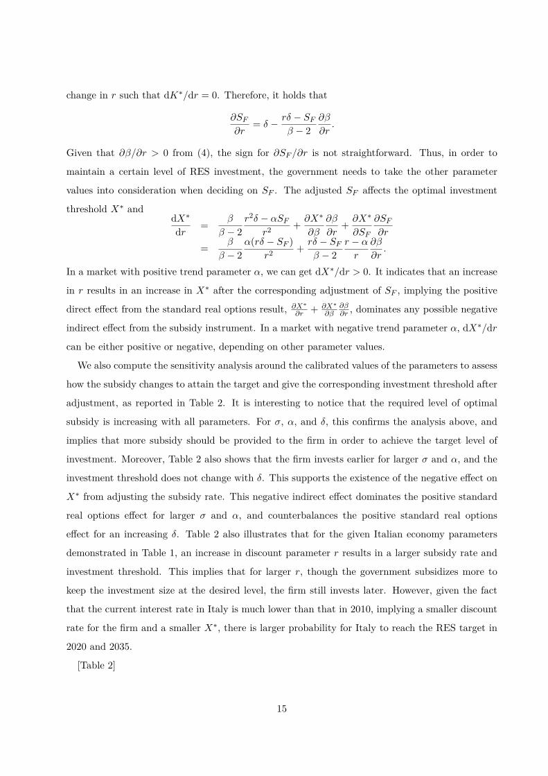
change in r such that dK∗/dr = 0. Therefore, it holds that

∂SF∂r

= δ − rδ − SFβ − 2

∂β

∂r.

Given that ∂β/∂r > 0 from (4), the sign for ∂SF /∂r is not straightforward. Thus, in order to

maintain a certain level of RES investment, the government needs to take the other parameter

values into consideration when deciding on SF . The adjusted SF affects the optimal investment

threshold X∗ anddX∗

dr = β

β − 2r2δ − αSF

r2 + ∂X∗

∂β

∂β

∂r+ ∂X∗

∂SF

∂SF∂r

= β

β − 2α(rδ − SF )

r2 + rδ − SFβ − 2

r − αr

∂β

∂r.

In a market with positive trend parameter α, we can get dX∗/dr > 0. It indicates that an increase

in r results in an increase in X∗ after the corresponding adjustment of SF , implying the positive

direct effect from the standard real options result, ∂X∗

∂r + ∂X∗

∂β∂β∂r , dominates any possible negative

indirect effect from the subsidy instrument. In a market with negative trend parameter α, dX∗/dr

can be either positive or negative, depending on other parameter values.

We also compute the sensitivity analysis around the calibrated values of the parameters to assess

how the subsidy changes to attain the target and give the corresponding investment threshold after

adjustment, as reported in Table 2. It is interesting to notice that the required level of optimal

subsidy is increasing with all parameters. For σ, α, and δ, this confirms the analysis above, and

implies that more subsidy should be provided to the firm in order to achieve the target level of

investment. Moreover, Table 2 also shows that the firm invests earlier for larger σ and α, and the

investment threshold does not change with δ. This supports the existence of the negative effect on

X∗ from adjusting the subsidy rate. This negative indirect effect dominates the positive standard

real options effect for larger σ and α, and counterbalances the positive standard real options

effect for an increasing δ. Table 2 also illustrates that for the given Italian economy parameters

demonstrated in Table 1, an increase in discount parameter r results in a larger subsidy rate and

investment threshold. This implies that for larger r, though the government subsidizes more to

keep the investment size at the desired level, the firm still invests later. However, given the fact

that the current interest rate in Italy is much lower than that in 2010, implying a smaller discount

rate for the firm and a smaller X∗, there is larger probability for Italy to reach the RES target in

2020 and 2035.

[Table 2]

15

6 Conclusion

We design a model for a firm investing in capacity for green energy in an uncertain economic

situation. The model allows for analyzing the effect of the governmental subsidy in the form of a

fixed feed-in-premium on the firm’s investment decision. In particular we find that a larger subsidy

induces the firm to invest earlier in less capacity.

This analysis allows to find the most suitable subsidy level to reach a certain environmental

target level as soon as possible. This goes as follows. First, the environmental target fixes the

required investment size. Based on this size, we can find the subsidy level and the investment

threshold. From the threshold, we can obtain the expected time to reach the environmental target.

Using the Italian data, we applied this model to determine the most suitable subsidy level to

reach the given environmental EU target in 2020 and 2035.

References

AEEG. Relazione annuale sullo stato dei servizi e sull’attivita svolta. Technical report, Roma,

2016.

Simona Bigerna and Paolo Polinori. Italian households»ş willingness to pay for green electricity.

Renewable and Sustainable Energy Reviews, 34:110–121, 2014.

Simona Bigerna, Carlo Andrea Bollino, and Silvia Micheli. The Sustainability of Renewable Energy

in Europe. 2015.

Trine Krogh Boomsma and Kristin Linnerud. Market and policy risk under different renewable

electricity support schemes. Energy, 89:435–448, 2015.

Trine Krogh Boomsma, Nigel Meade, and Stein-Erik Fleten. Renewable energy investments under

different support schemes: A real options approach. European Journal of Operational Research,

220(1):225–237, 2012.

Peter Broer and Gijsbert Zwart. Optimal regulation of lumpy investments. Journal of Regulatory

Economics, 44(2):177–196, 2013.

Michail Chronopoulos, Verena Hagspiel, and Stein-Erik Fleten. Stepwise Green Investment under

Policy Uncertainty. Energy Journal, 37(4):87–108, 2016.

16

Thomas Dangl. Investment and capacity choice under uncertain demand. European Journal of

Operational Research, 117(3):415–428, 1999.

Neal Detert and Koji Kotani. Real options approach to renewable energy investments in Mongolia.

Energy Policy, 56:136–150, 2013.

Avinash K Dixit and Robert S Pindyck. Investment under uncertainty. Princeton university press,

Princeton, 1994.

Amro M. Elshurafa, Shahad R. Albardi, Carlo Andrea Bollino, and Simona Bigerna. Estimating the

learning curve of solar pv balance-of-systems for over 20 countries. KAPSARC working paper,

2017.

European Commission. Communication from the Commission to the European Parliament, the

Council, the European Economic and Social Committee and the Committee of the Regions: A

policy framework for climate and energy in the period from 2020 to 2030. Technical report,

Brussels, 2014.

European Commission. Proposal for a directive of the European Parliament and of the Council

on the promotion of the use of energy from renewable sources (recast), COM(2016) 767 final/2

2016/0382 (COD). Technical report, Brussels, 2017.

Lewis Evans and Graeme Guthrie. Price-cap regulation and the scale and timing of investment.

The RAND Journal of Economics, 43(3):537–561, 2012.

Stein-Erik Fleten, Karl M Maribu, and Ivar Wangensteen. Optimal investment strategies in decen-

tralized renewable power generation under uncertainty. Energy, 32(5):803–815, 2007.

Stein-Erik Fleten, Kristin Linnerud, Peter Molnar, and Maria Tandberg Nygaard. Green electricity

investment timing in practice: Real options or net present value? Energy, 116:498–506, 2016.

Nadine Gatzert and Nikolai Vogl. Evaluating investments in renewable energy under policy risks.

Energy Policy, 95:238–252, 2016.

Verena Hagspiel, Kuno J M Huisman, and Peter M Kort. Volume flexibility and capacity investment

under demand uncertainty. International Journal of Production Economics, 178:95–108, 2016a.

17

Verena Hagspiel, Kuno J M Huisman, Peter M Kort, and Claudia Nunes. How to escape a declining

market: Capacity investment or Exit? European Journal of Operational Research, 254(1):40–50,

2016b.

Kuno J.M. Huisman and Peter M. Kort. Strategic capacity investment under uncertainty. The

RAND Journal of Economics, 46(2):376–408, 2015.

International Energy Agency. Medium-term renewable energy market report 2015: Market analysis

and forecasts to 2020. Technical report, Paris, 2015.

International Energy Agency. Energy policies of IEA countries - Italy 2016 review. Technical

report, Paris, 2016.

Lionel Nesta, Francesco Vona, and Francesco Nicolli. Environmental policies, competition and

innovation in renewable energy. Journal of Environmental Economics and Management, 67(3):

396 – 411, 2014.

Grzegorz Pawlina and Peter M Kort. Investment under uncertainty and policy change. Journal of

Economic Dynamics and Control, 29(7):1193–1209, 2005.

Ingmar Ritzenhofen and Stefan Spinler. Optimal design of feed-in-tariffs to stimulate renewable

energy investments under regulatory uncertainty — A real options analysis. Energy Economics,

53:76–89, 2016.

Xingang Wen, Peter M Kort, and Dolf Talman. Volume flexibility and capacity investment: a real

options approach. Journal of the Operational Research Society, 68(12):1633–1646, 2017.

Bert Willems and Gijsbert Zwart. Optimal regulation of network expansion. The RAND Journal

of Economics, 2017.

Mingming Zhang, Dequn Zhou, and Peng Zhou. A real options model for renewable energy invest-

ment with application to solar photovoltaic power generation in China. Energy Economics, 59:

213–226, 2016.

18

Table 1: Calibration of parameter values in 2010 for Italy.

Parameter Value Range

r 0.06 0.045 – 0.06

α 0.02 0.0185 – 0.0210

σ 0.07 0.007 – 0.008

δ 1750 1535 – 1770

η 0.00007

X0 11.4

19

Table 2: Sensitivity analysis of parameters σ, α, δ, and r, for policy targets 2020 and 2035: Optimal

SF to reach K∗ and the corresponding threshold X∗.

Target 2020 Target 2035

Optimal SF value 100.9 98.8

Optimal K∗ value 110.4 168.4

2020 2035 2020 2035

σ SF X∗ SF X∗ α SF X∗ SF X∗

0.05 99.5 14.0 96.6 21.3 0.018 99.5 14.6 96.7 22.3

0.07 100.9 13.0 98.8 19.9 0.019 100.3 13.8 97.8 21.1

0.09 102.3 12.1 100.8 18.5 0.02 100.9 13.0 98.8 19.9

0.095 102.6 11.9 101.3 18.2 0.021 101.6 12.3 99.8 18.7

0.1 102.9 11.7 101.8 17.9 0.022 102.2 11.6 100.7 17.7

2020 2035 2020 2035

δ SF X∗ SF X∗ r SF X∗ SF X∗

1650 94.9 13.0 92.8 19.9 0.045 78.7 8.6 78.7 13.1

1700 97.9 13.0 95.8 19.9 0.048 83.1 9.5 82.7 14.5

1750 100.9 13.0 98.8 19.8 0.055 93.5 11.6 92.0 17.7

1800 103.9 13.0 101.8 19.9 0.058 97.9 12.5 96.1 19.0

1850 106.9 13.0 104.8 19.9 0.06 100.9 13.0 98.8 19.9

20

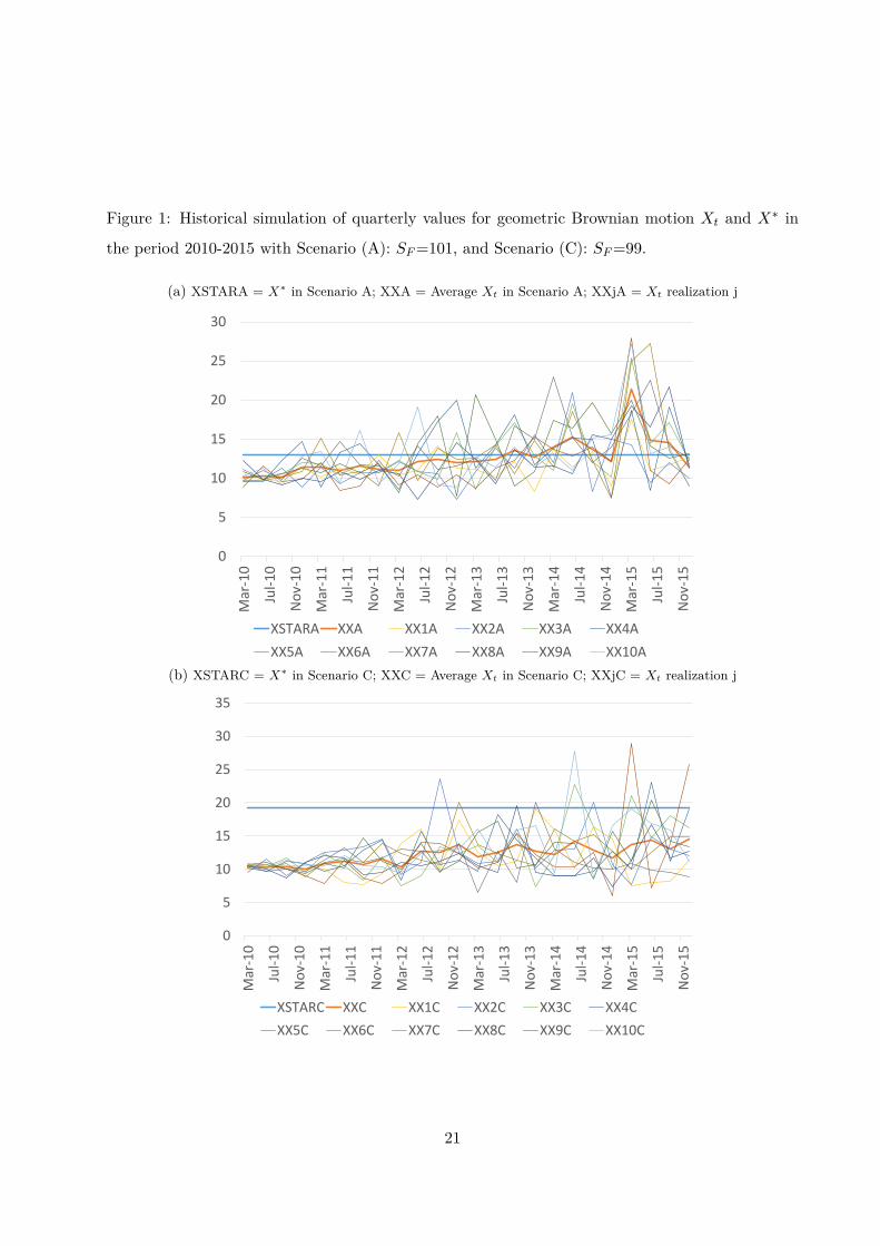
Figure 1: Historical simulation of quarterly values for geometric Brownian motion Xt and X∗ in

the period 2010-2015 with Scenario (A): SF=101, and Scenario (C): SF=99.

(a) XSTARA = X∗ in Scenario A; XXA = Average Xt in Scenario A; XXjA = Xt realization j

0

5

10

15

20

25

30

Mar

-10

Jul-1

0

Nov

-10

Mar

-11

Jul-1

1

Nov

-11

Mar

-12

Jul-1

2

Nov

-12

Mar

-13

Jul-1

3

Nov

-13

Mar

-14

Jul-1

4

Nov

-14

Mar

-15

Jul-1

5

Nov

-15

XSTARA XXA XX1A XX2A XX3A XX4AXX5A XX6A XX7A XX8A XX9A XX10A

(b) XSTARC = X∗ in Scenario C; XXC = Average Xt in Scenario C; XXjC = Xt realization j

0

5

10

15

20

25

30

35

Mar

-10

Jul-1

0

Nov

-10

Mar

-11

Jul-1

1

Nov

-11

Mar

-12

Jul-1

2

Nov

-12

Mar

-13

Jul-1

3

Nov

-13

Mar

-14

Jul-1

4

Nov

-14

Mar

-15

Jul-1

5

Nov

-15

XSTARC XXC XX1C XX2C XX3C XX4CXX5C XX6C XX7C XX8C XX9C XX10C

21

Figure 2: Quarterly percentage realization of X∗ in the period 2010-2015 for Scenario (A): SF=101,

and Scenario (C): SF=99.

0

0.2

0.4

0.6

0.8

1

1.2M

ar-1

0

Jul-1

0

Nov

-10

Mar

-11

Jul-1

1

Nov

-11

Mar

-12

Jul-1

2

Nov

-12

Mar

-13

Jul-1

3

Nov

-13

Mar

-14

Jul-1

4

Nov

-14

Mar

-15

Jul-1

5

Nov

-15

DDA DDC

Figure 3: Percentage realization of X∗ in the period 2016-2035 under different subsidy rates.

0

0.2

0.4

0.6

0.8

1

1.2parameter SF

DDA DDB DDC DDD DDE

22

Figu

re4:

Para

met

erse

nsiti

vity

and

perc

enta

gere

aliz

atio

nofX∗ :

Ann

ualv

alue

sin

the

perio

d20

16-2

035.

(a)σ

0

0.1

0.2

0.3

0.4

0.5

0.6

0.7

0.8

para

met

er σ

DDA

DDB

DDC

DDD

DDE

(b)α

0

0.1

0.2

0.3

0.4

0.5

0.6

para

met

er α

DDA

DDB

DDC

DDD

DDE

(c)δ

0

0.1

0.2

0.3

0.4

0.5

0.6

0.7

0.8

para

met

er δ

DDA

DDB

DDC

DDD

DDE

(d)r

0

0.1

0.2

0.3

0.4

0.5

0.6

0.7

0.8

para

met

er r

DDA

DDB

DDC

DDD

DDE

23