Green’s Functions Application for ComputerModeling in Electromagnetics

Sergey N. Shabunin1, Victor A. Chechetkin1

1Ural Federal University, Ekaterinburg, Russian Federations.n.shabunin@urfu.ru, v.a.chechetkin@urfu.ru

Abstract. Features of application of the Green’s function method in theCartesian, cylindrical, and spherical coordinate systems are considered.The equivalent circuit method is used to describe the layered structure.To simulate propagation of the electromagnetic waves in each layer, ma-trices of the layer transmission and boundaries are applied. It is shownthat the transfer matrices of the boundaries in the Cartesian and spher-ical coordinate systems are unit matrices. Different types of load modelthe boundaries of areas. The proposed approach allows one to create uni-versal algorithms with common modules for solving various electromag-netic problems. Those are excitation and propagation of waves, antennaradiation and diffraction associated with flat, cylindrical, and sphericallayered structures with an arbitrary number of layers, permittivity, andpermeability. Some examples of using the Green’s functions in softwareproducts are presented.

Keywords: electromagnetics, Greens function, scattering, radiation, al-gorithms

1 Introduction

The tasks of electromagnetic modeling are the integral part of most projects re-lated to telecommunications, navigation, and radar. These can be particular onesrelated to design of antennas, antenna arrays, high frequency circuits, elementsof radio-electronics, etc. Tasks can be very different, such as synthesis of thenon-reflective or selectively transmitting materials, solution of electromagneticscattering problem at objects, solution of problem of radio wave propagation ininhomogeneous media, etc. At the present stage, taking into account the greatcapabilities of computing technology, specialized electromagnetic simulation soft-ware (such as Ansys HFSS, FEKO, CST Microwave Studio) is widely used [13].However, solution of the electromagnetic radiation and diffraction problems isusually associated with partition of the analyzed objects into the simplest vol-umes or surfaces and the subsequent solution of systems of extremely high-orderalgebraic equations. This leads to significant costs of the CPU time. This is espe-cially apparent when optimizing the geometry of objects or the electro-physicalcharacteristics of the materials is used. Good initial approximation in optimizingthe electrodynamic characteristics of the objects under study is actual.

63

Along with the use of special software, methods based on an analytical ap-proach are also used, but recently not so wide. This fact is due to the rathercomplex preparatory work and high requirements for knowledge of mathemat-ics in derivation of expressions suitable for programming. Another constraint isthe limitations in the choice of the shape of the analyzed objects for compactcomputational formulas. The analyzed objects should be fitted to the existingcoordinate systems. The preferable forms are the plane-parallel structures, par-allelepipeds, cylinders, spheres and their fragments. This requirement is due tothe need to perform the integration operation over the coordinate surfaces. De-spite these limitations, analytical methods can be considered as a powerful toolfor solving many electromagnetic problems, and, also, as a first step in solvingcomplex problems using electromagnetic simulation software. For example, if thetask is to synthesize an object with a minimum scattering diameter, the initialsynthesis of the non-reflective coatings can be performed using the analytical ap-proaches. The gain increases with increasing electrical dimensions of the objectsunder investigation.

One of the most common analytical methods for solving problems of electro-dynamics is the Green’s function method. Being a solution of the inhomogeneousMaxwell equations for a source in the form of a delta function, the Green’s func-tions allow one to calculate a vector field at an arbitrary point in space. Bytaking into account all the excitation points, one can construct the pattern ofthe electromagnetic field distribution. Another advantage of this method is thatthe field can be counted only in the required areas that save the CPU time.When obtaining Green’s functions, the boundary conditions at the boundariesof the regions and the radiation conditions at infinity are taken into account.The method is a rigorous electrodynamic one.

This article applies the Green’s functions to layered structures in the Carte-sian, cylindrical, and spherical regions and shows the features of the use of theGreen’s functions apparatus when using the model of equivalent electrical cir-cuits to describe the layered structure. The results of electromagnetic modelingare given on the example of synthesis of the non-reflective coatings and solutionof the diffraction problems.

2 Green’s functions in generalized coordinates

In general, the task of calculating the electromagnetic field excited by the extra-neous electric J(r′) and/or magnetic M(r′) currents is written in the followingform:

E(r) =

∫V ′

[Γ 11(r, r′)J(r′) + Γ 12(r, r′)M(r′)

]dv′, (1)

where Γ 11(r, r′), Γ 12(r, r′) are the electric and “transfer” Green’s function,respectively [4]. Similarly, expression for calculation of the magnetic field com-ponent is written. Vector r′ defines the source point, vector r defines the obser-vation point. Integration in (1) is performed over the region of the source.

64

For an unlimited homogeneous space, the Green’s function for electric fieldexcited by electric current has a simple form:

Γ 11(r, r′) =1

4π

exp(−jk|r − r′|)|r − r′|

. (2)

If the space is limited, for example, by a conducting plane, the Green’s func-tion becomes more complicated. Moreover, when constructing the functions, theused coordinate system should be taken into account.

All electromagnetic problems of excitation, radiation, and scattering aresolved with a model of electric and magnetic currents. For example, the cur-rents on the surface of the printed patch antenna are of the electric type. Thecurrents in the slot antenna are magnetic ones. The field formed by the hornantenna is calculated as the radiation of Huygens elements in the aperture ofthe horn, whose amplitude and phase are determined by the parameters of thehorn. The Huygens element itself is modeled by a pair of the orthogonal electricand magnetic dipoles. The diffraction problems are reduced to the problems ofradiation by the currents induced on the irradiated objects.

Greens functions are especially complex in the inhomogeneous and layeredmedia. To simplify the Green’s functions, the electromagnetic field is presentedas a superposition of the electric and magnetic waves [5]. Separation of wavetypes is carried out relatively to the selected axis of the coordinate system.In the Cartesian system, all axes are equivalent. Let’s choose the z axis. Theelectromagnetic field is decomposed into a spatial spectrum of the plane waves.In a cylindrical system, separation occurs relatively to the z axis. The field isdecomposed into a spectrum of the spatial longitudinal waves with respect tothis axis: either radially propagating or azimuthally propagating waves. Thechoice of decomposition depends on the problem to be solved. In the sphericalcoordinate system, the radial axis is selected as the separation one. The fieldis formed by the spatial harmonics of waves propagating along the angular orradial coordinates.

Layer structure in all coordinate systems is modeled by the equivalent elec-trical circuits. The validity of this approach follows from solution of the inho-mogeneous system of the Maxwell equations. In this case, the transverse fieldcomponents are expressed in terms of the components associated with the de-composition axis. The system of 6 algebraic equations is divided into two inde-pendent systems of equations. For example, in the cylindrical coordinates, for ahomogeneous layer, this system looks as follows:

− d

dr(Eezmh) = −j γ

2Z0

εrk20(k0rH

eϕmh)− hZ0

εk0JE exrmh − JM ex

ϕmh ,

− d

dr(k0rH

eϕmh) = j

εk20Z0γ2

r

[k2 − h2 −

(mr

)2]Eezmh + k0rJ

E exzmh−

−mhk0γ

JE exϕmh +

εk0γ2Z0

mJM exrmh .

(3)

65

The type of the reduced system of equations resembles the system of equa-tions for the voltage and current in a long line as follows:

− d

drVE = jZEχIE + νEct,

− d

drIE = jYEχVE + iEct.

(4)

Comparing (3) and (4) you can get the following expressions for equivalentelectric circuit:

VE = Eezmh, IE = −k0rHeϕmh, χ

2 = k2−h2−(mr

)2, ZE =

γ2

k20εr

Z0√k2 − h2 −

(mr

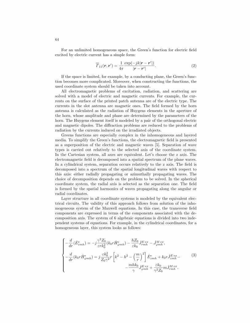
)2 .Since we have electric and magnetic wave, the decomposition of two E and

H-lines in electric equivalent circuit is used (Fig. 1). Similar operations havebeen carried out for other coordinate systems. The generalized coordinate τ cor-responds to the coordinate z, ρ, or r in the Cartesian, cylindrical, and sphericalcoordinate system, respectively.

Fig. 1. A homogeneous layer and its electric circuit model

Let us note that the propagation constant and the characteristic impedancein the equivalent circuit in the cylindrical and spherical coordinate systems de-pend on the radial component. In the Cartesian coordinate system, they remainconstant.

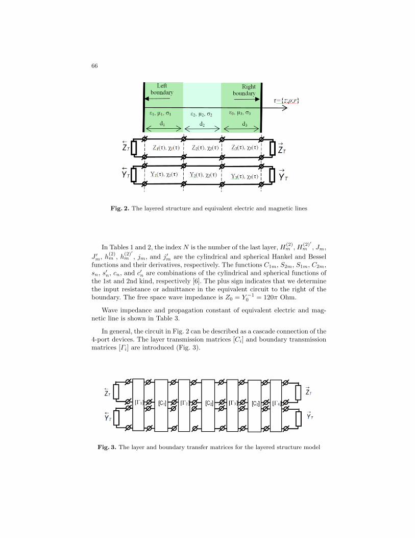
If the medium is heterogeneous and it is modeled by a layered structure,the equivalent circuit is the cascade connection of line segments with different

parameters (Fig. 2). The directional resistances←−Z T ,

−→Z T and conductivities

←−Y T ,

−→Y T , as the terminal loads are used for the region boundaries modeling (Table 1and Table 2).

66

Fig. 2. The layered structure and equivalent electric and magnetic lines

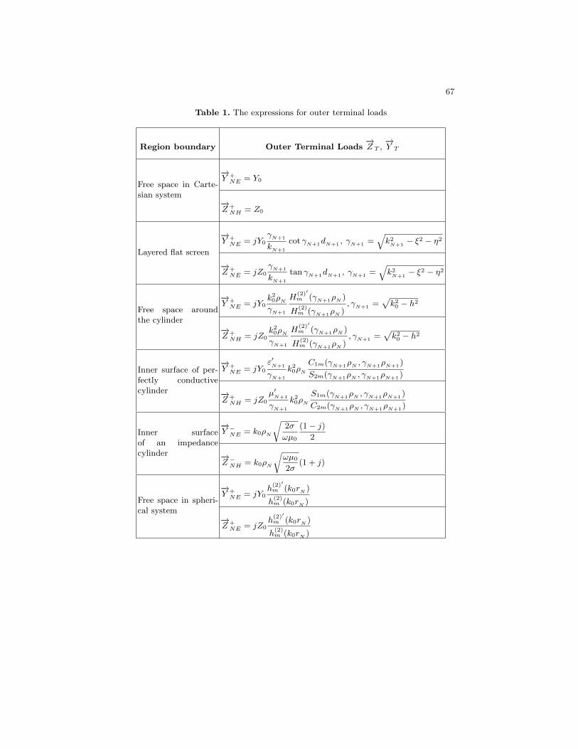
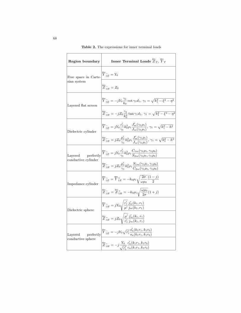
In Tables 1 and 2, the index N is the number of the last layer, H(2)m , H

(2)′

m , Jm,

J ′m, h(2)m , h

(2)′

m , jm, and j′m are the cylindrical and spherical Hankel and Besselfunctions and their derivatives, respectively. The functions C1m, S2m, S1m, C2m,sn, s′n, cn, and c′n are combinations of the cylindrical and spherical functions ofthe 1st and 2nd kind, respectively [6]. The plus sign indicates that we determinethe input resistance or admittance in the equivalent circuit to the right of theboundary. The free space wave impedance is Z0 = Y −10 = 120π Ohm.

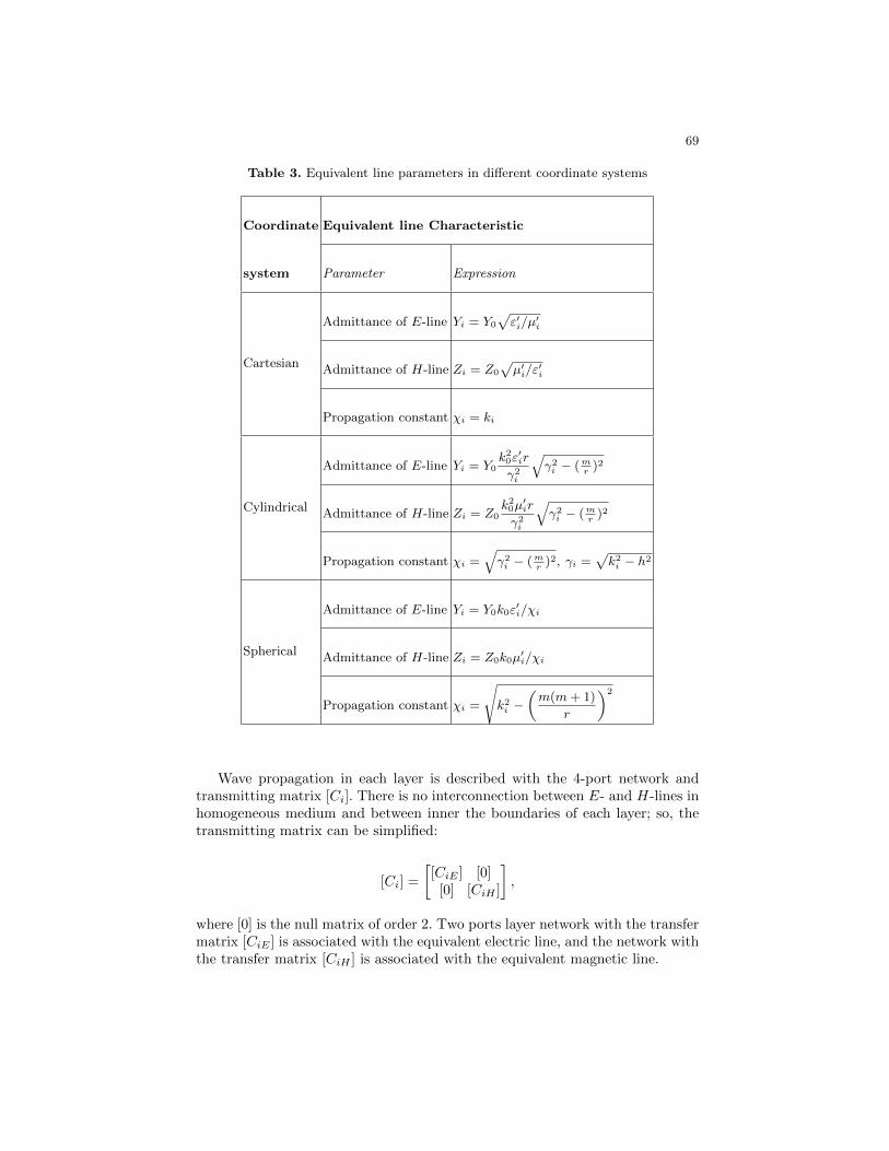
Wave impedance and propagation constant of equivalent electric and mag-netic line is shown in Table 3.

In general, the circuit in Fig. 2 can be described as a cascade connection of the4-port devices. The layer transmission matrices [Ci] and boundary transmissionmatrices [Γi] are introduced (Fig. 3).

Fig. 3. The layer and boundary transfer matrices for the layered structure model

67

Table 1. The expressions for outer terminal loads

Region boundary Outer Terminal Loads−→Z T ,

−→Y T

Free space in Carte-sian system

−→Y +

NE = Y0

−→Z +

NH = Z0

Layered flat screen

−→Y +

NE = jY0

γN+1

kN+1

cot γN+1dN+1 , γN+1 =√k2N+1− ξ2 − η2

−→Z +

NE = jZ0

γN+1

kN+1

tan γN+1dN+1 , γN+1 =√k2N+1− ξ2 − η2

Free space aroundthe cylinder

−→Y +

NE = jY0k20ρN

γN+1

H(2)′m (γN+1ρN )

H(2)m (γN+1ρN )

, γN+1 =√k20 − h2

−→Z +

NH = jZ0k20ρN

γN+1

H(2)′m (γN+1ρN )

H(2)m (γN+1ρN )

, γN+1 =√k20 − h2

Inner surface of per-fectly conductivecylinder

−→Y +

NE = jY0

ε′N+1

γN+1

k20ρN

C1m(γN+1ρN , γN+1ρN+1)

S2m(γN+1ρN , γN+1ρN+1)

−→Z +

NH = jZ0

µ′N+1

γN+1

k20ρN

S1m(γN+1ρN , γN+1ρN+1)

C2m(γN+1ρN , γN+1ρN+1)

Inner surfaceof an impedancecylinder

−→Y −NE = k0ρN

√2σ

ωµ0

(1− j)2

−→Z −NH = k0ρN

√ωµ0

2σ(1 + j)

Free space in spheri-cal system

−→Y +

NE = jY0h(2)′m (k0rN )

h(2)m (k0rN )

−→Z +

NE = jZ0h(2)′m (k0rN )

h(2)m (k0rN )

68

Table 2. The expressions for inner terminal loads

Region boundary Inner Terminal Loads←−Z T ,

←−Y T

Free space in Carte-sian system

←−Y −1E = Y0

←−Z −1H = Z0

Layered flat screen

←−Y −1E = −jY0

γ1k0

cot γ1d1, γ1 =√k21 − ξ2 − η2

←−Z −1H = −jZ0

γ1k20

tan γ1d1, γ1 =√k21 − ξ2 − η2

Dielectric cylinder

←−Y −1E = jY0

ε′1γ1k20ρ1

J ′m(γ1ρ1)

Jm(γ1ρ1), γ1 =

√k21 − h2

←−Z −1H = jZ0

µ′1γ1k20ρ1

J ′m(γ1ρ1)

Jm(γ1ρ1), γ1 =

√k21 − h2

Layered perfectlyconductive cylinder

←−Y −1E = jY0

ε′1γ1k20ρ1

C1m(γ1ρ1, γ1ρ0)

S2m(γ1ρ1, γ1ρ0)

←−Z −1H = jZ0

µ′1γ1k20ρ1

S1m(γ1ρ1, γ1ρ0)

C2m(γ1ρ1, γ1ρ0)

Impedance cylinder

←−Y −1E =

←−Y +

1E = −k0ρ1√

2σ

ωµ0

(1− j)2

←−Z −1H =

←−Z +

1H = −k0ρ1√ωµ0

2σ(1 + j)

Dielectric sphere

←−Y −1H = jY0

√ε′1µ′j′m(k1, r1)

jm(k1, r1)

←−Z −1H = jZ0

√µ′

ε′1

j′m(k1, r1)

jm(k1, r1)

Layered perfectlyconductive sphere

←−Y −1E = −jY0

√ε′1s′n(k1r1, k1r0)

sn(k1r1, k1r0)

←−Z −1H = −j Y0√

ε′1

c′n(k1r1, k1r0)

cn(k1r1, k1r0)

69

Table 3. Equivalent line parameters in different coordinate systems

Coordinate

system

Equivalent line Characteristic

Parameter Expression

Cartesian

Admittance of E-line Yi = Y0

√ε′i/µ

′i

Admittance of H-line Zi = Z0

√µ′i/ε

′i

Propagation constant χi = ki

Cylindrical

Admittance of E-line Yi = Y0k20ε′ir

γ2i

√γ2i − (m

r)2

Admittance of H-line Zi = Z0k20µ

′ir

γ2i

√γ2i − (m

r)2

Propagation constant χi =√γ2i − (m

r)2, γi =

√k2i − h2

Spherical

Admittance of E-line Yi = Y0k0ε′i/χi

Admittance of H-line Zi = Z0k0µ′i/χi

Propagation constant χi =

√k2i −

(m(m+ 1)

r

)2

Wave propagation in each layer is described with the 4-port network andtransmitting matrix [Ci]. There is no interconnection between E- and H-lines inhomogeneous medium and between inner the boundaries of each layer; so, thetransmitting matrix can be simplified:

[Ci] =

[[CiE ] [0]

[0] [CiH ]

],

where [0] is the null matrix of order 2. Two ports layer network with the transfermatrix [CiE ] is associated with the equivalent electric line, and the network withthe transfer matrix [CiH ] is associated with the equivalent magnetic line.

70

The boundary transmission matrix in the Cartesian and spherical coordinatesystems is the identity matrix. But in the cylindrical coordinates, these matricescan be complicated:

[Γi] =

1 0 0 00 1 0 −NiNi 0 1 00 0 0 1

,where Ni =

mh

k0

(1

γ2i− 1

γ2i+1

), γi =

√k2i − h2.

The suggested layer structure model allows one to develop algorithms for theelectromagnetic field calculation based on common modules for different kind ofradiation, propagation, and scattering problems.

3 Green’s functions in basic coordinate systems

The Greens functions according to the electromagnetic field decomposition ontothe electric and magnetic waves have two parts. The first one takes into accountthe layer structure and it is characteristic part of the functions. The second partdescribes field in the perpendicular (to the layers) directions. These surfaces maybe limited or unlimited by conducting surfaces.

In the Cartesian coordinates, the Greens functions are as follows:

Γ ij(x, y, z, x′, y′, z′) = jωµ0

∞∫−∞

∞∫−∞

F {g(z; z′), f(z; z′)}Gt(x, y;x′, y′)dξdθ, (5)

where for unlimited space along the x and y coordinates

Gt(x, y;x′, y′) =1

4πe−iξ(x−x

′)e−iθ(y−y′).

In (5), the characteristic functions and are solutions of the differential equa-tions with the proper boundary conditions:

∂2f(z, z′)

∂z2+ γ2f(z, z′) = δ(z − z′),

∂2g(z, z′)

∂z2+ γ2g(z, z′) = δ(z − z′).

If the boundary is the perfect conductor, we have at this section f(z, z′) =∂f(z, z′)

∂z= 0.

For the cylindrical coordinate system, the Greens functions are defined asfollows:

Γ ij(ρ, ϕ, z, ρ′, ϕ′, z′) = −j ωµ0

2π

∞∑m=−∞

∞∫−∞

F {gm(ρ; ρ′), fm(ρ; ρ′)}Gt(m,h, ϕ, z;ϕ′, z′)dh,

71

where Gt(m,h, ϕ, z;ϕ′, z′) =

1

2πe−jm(ϕ−ϕ′)e−jh(z−z

′).

The characteristic functions gm(ρ; ρ′) and fm(ρ; ρ′) are solutions of the dif-ferential equations:

1

ρ

d

dρ

(ρdgm(ρ; ρ′)

dρ

)+

(k2 − h2 − m2

ρ2

)gm(ρ; ρ′) = −δ(ρ− ρ′),

1

ρ

d

dρ

(ρdfm(ρ; ρ′)

dρ

)+

(k2 − h2 − m2

ρ2

)fm(ρ; ρ′) = −δ(ρ− ρ′).

If the spherical structures are under consideration, the Greens functions aredefined as:

Γ ij(θ, ϕ, r; θ′, ϕ′, r′) = jωµ0

∞∑n=0

n∑m=−n

F{gn(r; r′), fn(r; r′)}Gt(m,n, θ, ϕ; θ′, ϕ′),

where Gt(m,n, θ, ϕ; θ′, ϕ′) =1

4πΦ{Pmn (cos θ)e−jmϕ, Pmn (cos θ′)ejmϕ

′}

.

The spherical harmonics are calculated using the associated Legendre poly-nomials Pmn (cos θ).

The characteristic functions are solutions of the inhomogeneous equations:

∂2gn(r, r′)

∂r2+ k2gn(r, r′) = −δ(r − r′),

∂2fn(r, r′)

∂r2+ k2fn(r, r′) = −δ(r − r′).

Thus, the Greens functions for three main coordinate systems (Cartesian,cylindrical and spherical) are given. A wide class of electromagnetic excitation,radiation, and diffraction problems can be solved using the appropriate distri-bution of extraneous currents. Using the analytical approaches allows one sig-nificantly speed up the calculation in electromagnetics.

4 Greens function application in electromagnetic softwaredevelopment

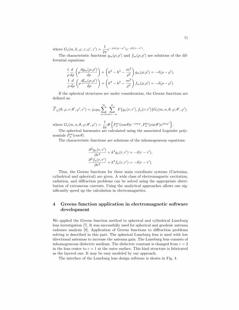
We applied the Greens function method to spherical and cylindrical Luneburglens investigation [7]. It was successfully used for spherical and geodesic antennaradomes analysis [8]. Application of Greens functions to diffraction problemssolving is described in this part. The spherical Luneburg lens is used with lowdirectional antennas to increase the antenna gain. The Luneburg lens consists ofinhomogeneous dielectric medium. The dielectric constant is changed from ε = 2in the lens center to ε = 1 at the outer surface. This kind structure is fabricatedas the layered one. It may be easy modeled by our approach.

The interface of the Luneburg lens design software is shown in Fig. 4.

72

Fig. 4. The interface of software for the Luneburg lens radiation analysis

Radiation pattern for the main and cross-polarized components are calcu-lated. Several types of low directional antennas as a Huygens element, a dipolewith conducting screen, and crossed dipoles may be used as the lens irradiator.The high speed of calculations is confirmed by Table 4, in which the processingtime for radiation pattern computation and different electrical outer radius k0a isshown. In comparison with the traditional software, the calculation is performedby 2–3 orders faster.

Table 4. Processing time of the Luneburg lens antenna radiation calculation

k0a t, sec

2π 1.8

4π 2.3

6π 3.1

12π 12.2

20π 30.3

28π 43.5

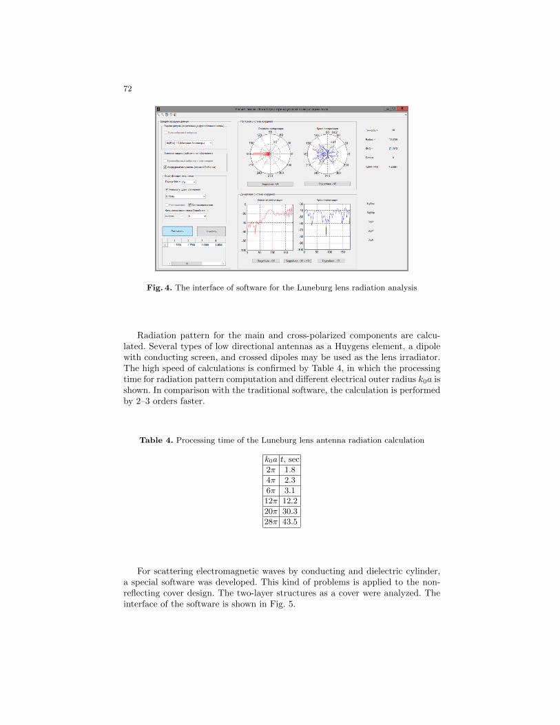
For scattering electromagnetic waves by conducting and dielectric cylinder,a special software was developed. This kind of problems is applied to the non-reflecting cover design. The two-layer structures as a cover were analyzed. Theinterface of the software is shown in Fig. 5.

73

Fig. 5. The interface of software for scattering by covered cylinder

5 Conclusion

TThe spectral-domain full-wave approach based on Greens function method forlayered magneto-dielectric structure analysis is described. The Green’s functionsfor electromagnetic excitation problems in Cartesian, cylindrical and sphericalcoordinate systems are presented. The equivalent circuit model for layered struc-tures analysis is applied. The 4-port network with transmitting matrix is usedfor boundary between layers description. The same kind of matrices was ap-plied for wave propagation analysis in each layer. The solution remains correctfor any type of isotropic magneto-dielectrics. The suggested approach was usedfor electromagnetic software developing. The procedure of calculation and opti-mization electromagnetic radiation and scattering is significantly accelerated incomparing with commercial software.

Acknowledgments

The work was supported by the Act 211 of the Russian Federation Government,contract 02.A03.21.0006.

References

1. L. Sevgi, Electromagnetic Modeling and Simulation. Wiley-IEEE Press (2014)2. J. Volakis, Antenna Engineering Handbook. McGraw-Hill Education (2007)3. C.A. Balanis, Antenna Theory: Analysis and Design. Wiley (2016)

74

4. L. B. Felsen, N. Marcuvitz, Radiation and Scattering of Waves. Englewood Cliffs:Prentice Hall. (1973)

5. D. B. Davidson, Computational Electromagnetics for RF and Microwave Engineer-ing. Cambridge University Press. (2010)

6. S. Dailis, S. Shabunin. Microstrip antennas on metallic cylinder covered with radi-ally inhomogeneous magnetodielectric. Proc. 9th Int. Wroclaw Symp. on Electrom.Compatib., June 16-19. Wroclaw. Part 1, 271–277 (1988)

7. S. Knyazev, A. Korotkov, B. Panchenko, S. Shabunin. Investigation of sphericaland cylindrical Luneburg lens antennas by the Green’s function method. IOP Con-ference Series: Materials Science and Engineering, 120 (1), 012011 (2016)

8. A. Karpov, S. Knyazev, L. Lesnaya, S. Shabunin. Sandwich Spherical and GeodesicAntenna Radomes Analysis. Proc. of the 10th European Conference on Antennasand Propagation (EuCAP 2016), Davos, Switzerland, 1–5 (2016)