Embed Size (px)
DESCRIPTION
Green's function solution to subsurface light transport for BRDF computation. Charly Collin – Ke Chen – Ajit Hakke-Patil Sumanta Pattanaik – Kadi Bouatouch. Painted materials:. Painted materials:. Painted materials:. Painted materials:. Our goal:. - PowerPoint PPT Presentation
Citation preview
Green's function solution to subsurface light transport for BRDF computation
Charly Collin – Ke Chen – Ajit Hakke-PatilSumanta Pattanaik – Kadi Bouatouch
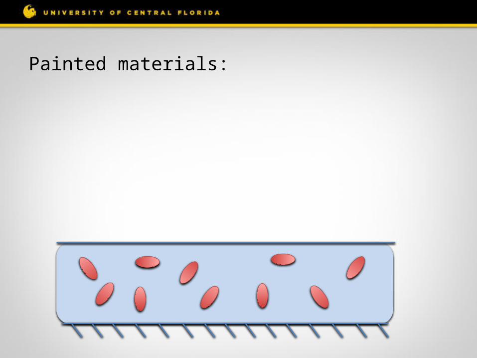
Painted materials:
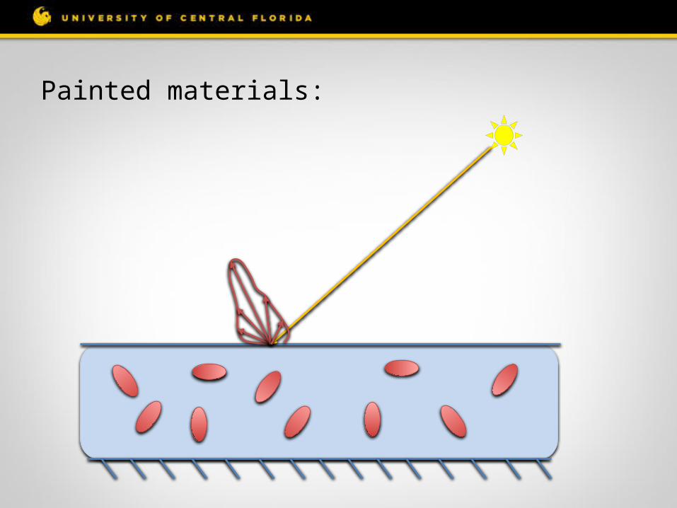
Painted materials:
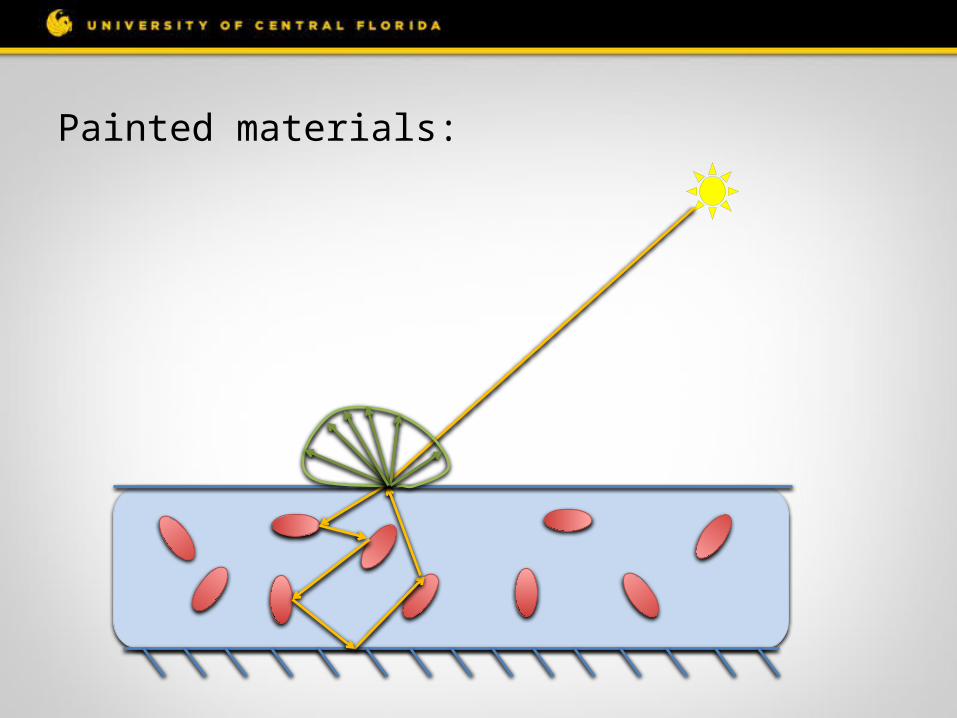
Painted materials:
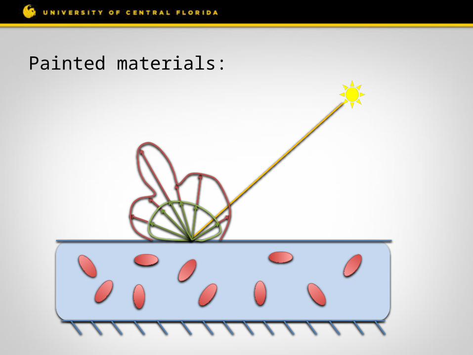
Painted materials:
Our goal:
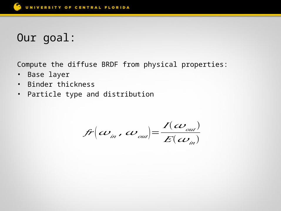
𝑓𝑟 (𝜔𝑖𝑛 ,𝜔𝑜𝑢𝑡 )=𝐼 (𝜔𝑜𝑢𝑡)𝐸 (𝜔 𝑖𝑛)
• Base layer• Binder thickness• Particle type and distribution
Compute the diffuse BRDF from physical properties:
BRDF Computation
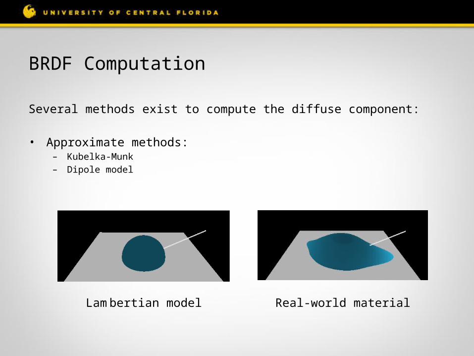
Several methods exist to compute the diffuse component:
• Approximate methods:– Kubelka-Munk– Dipole model
Lam bertian model Real-world material
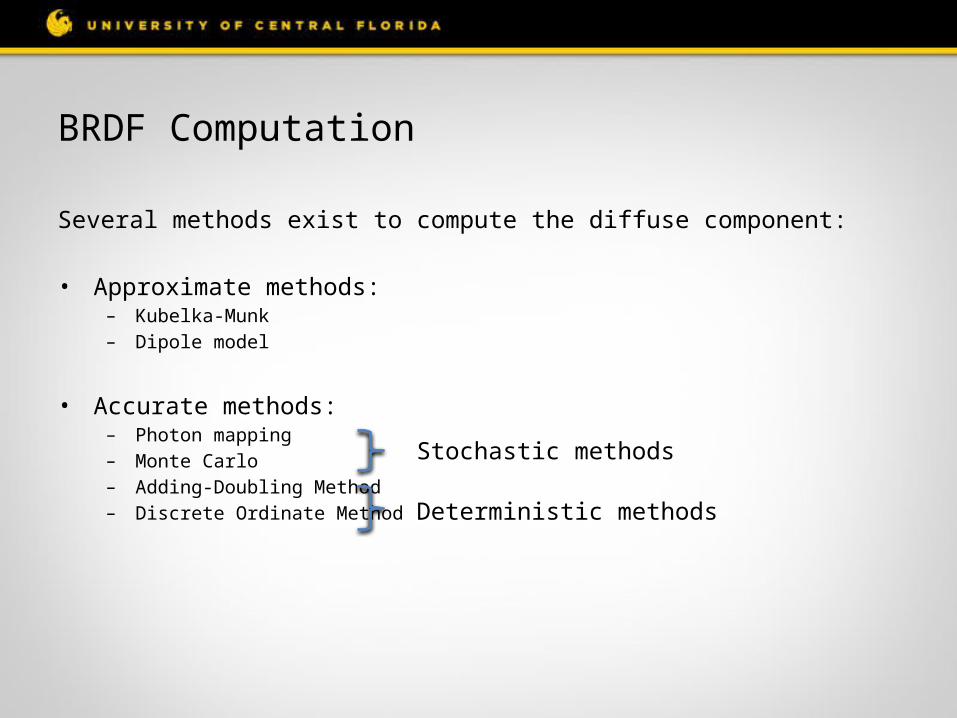
Several methods exist to compute the diffuse component:
• Approximate methods:– Kubelka-Munk– Dipole model
• Accurate methods:– Photon mapping– Monte Carlo– Adding-Doubling Method– Discrete Ordinate Method
BRDF Computation
Stochastic methods
Deterministic methods
BRDF Computation
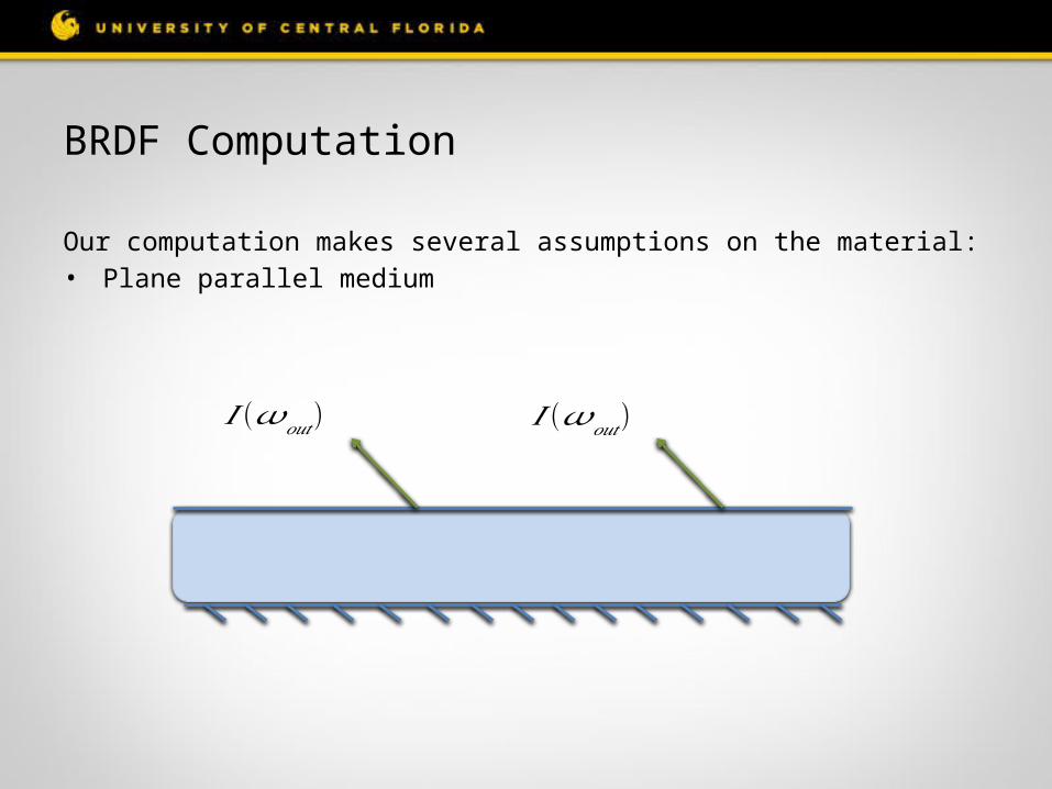
𝐼 (𝜔𝑜𝑢𝑡) 𝐼 (𝜔𝑜𝑢𝑡)
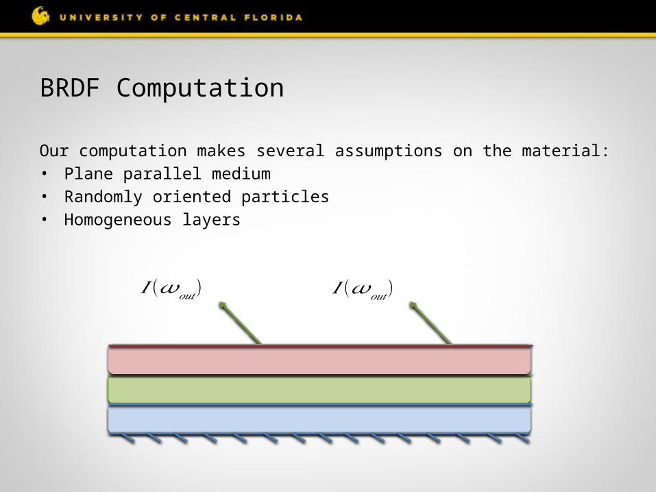
Our computation makes several assumptions on the material:• Plane parallel medium
BRDF Computation
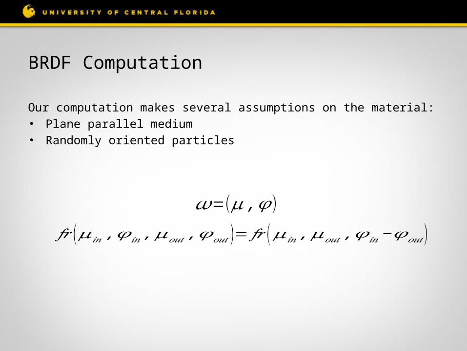
Our computation makes several assumptions on the material:• Plane parallel medium• Randomly oriented particles
𝑓𝑟 (𝜇𝑖𝑛 ,𝜑𝑖𝑛 ,𝜇𝑜𝑢𝑡 ,𝜑𝑜𝑢𝑡 )= 𝑓𝑟 (𝜇𝑖𝑛 ,𝜇𝑜𝑢𝑡 ,𝜑𝑖𝑛−𝜑 𝑜𝑢𝑡 )
𝜔=(𝜇 ,𝜑 )
BRDF Computation
Our computation makes several assumptions on the material:• Plane parallel medium• Randomly oriented particles• Homogeneous layers
𝐼 (𝜔𝑜𝑢𝑡) 𝐼 (𝜔𝑜𝑢𝑡)
BRDF Computation
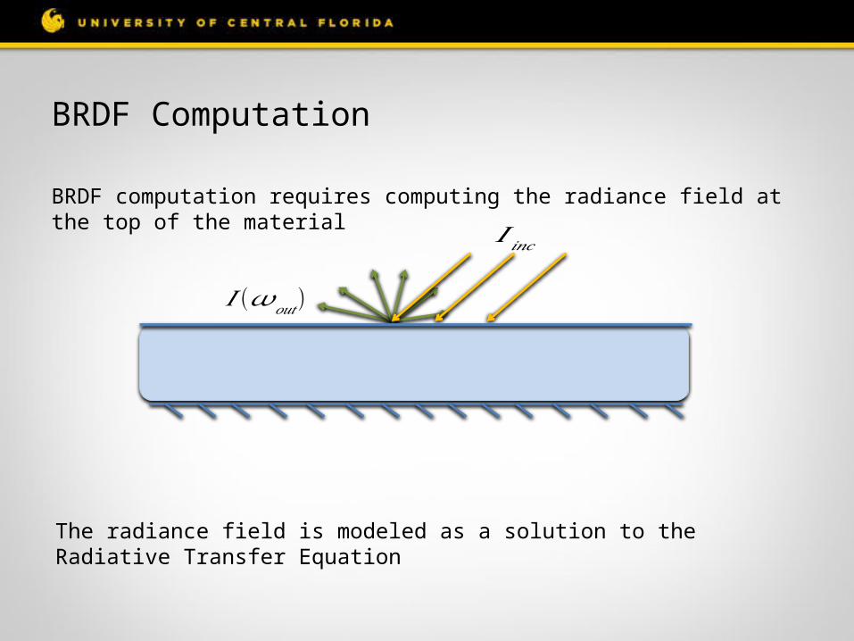
BRDF computation requires computing the radiance field at the top of the material
The radiance field is modeled as a solution to the Radiative Transfer Equation
𝐼 𝑖𝑛𝑐
𝐼 (𝜔𝑜𝑢𝑡)
Radiative Transfer Equation
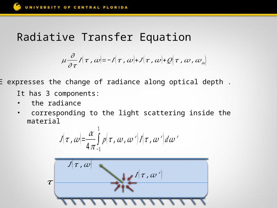
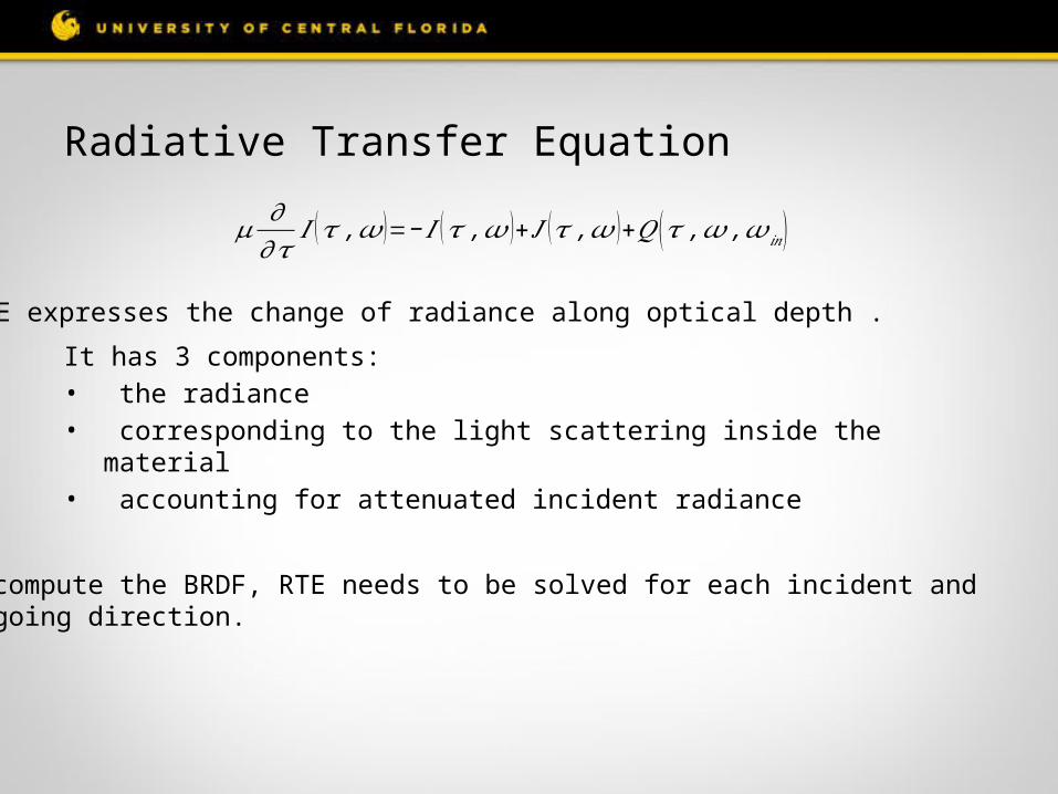
It has 3 components:• the radiance• corresponding to the light scattering inside the material
RTE expresses the change of radiance along optical depth .
𝐽 (𝜏 ,𝜔 )= 𝛼4 𝜋∫
− 1
1
𝑝 (𝜏 ,𝜔 ,𝜔 ′ ) 𝐼 (𝜏 ,𝜔 ′ )𝑑𝜔 ′
𝜏
𝐽 (𝜏 ,𝜔 )𝐼 (𝜏 ,𝜔 ′ )
𝜇𝜕𝜕𝜏
𝐼 (𝜏 ,𝜔 )=− 𝐼 (𝜏 ,𝜔 )+ 𝐽 (𝜏 ,𝜔 )+𝑄 (𝜏 ,𝜔 ,𝜔 𝑖𝑛)
Radiative Transfer Equation
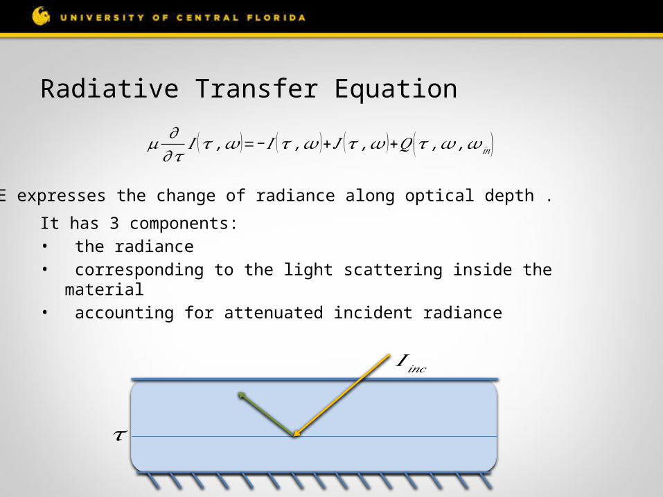
It has 3 components:• the radiance• corresponding to the light scattering inside the material• accounting for attenuated incident radiance
RTE expresses the change of radiance along optical depth .
𝜏
𝐼 𝑖𝑛𝑐
𝜇𝜕𝜕𝜏
𝐼 (𝜏 ,𝜔 )=− 𝐼 (𝜏 ,𝜔 )+ 𝐽 (𝜏 ,𝜔 )+𝑄 (𝜏 ,𝜔 ,𝜔 𝑖𝑛)
Radiative Transfer Equation
It has 3 components:• the radiance• corresponding to the light scattering inside the material• accounting for attenuated incident radiance
RTE expresses the change of radiance along optical depth .
𝜇𝜕𝜕𝜏
𝐼 (𝜏 ,𝜔 )=− 𝐼 (𝜏 ,𝜔 )+ 𝐽 (𝜏 ,𝜔 )+𝑄 (𝜏 ,𝜔 ,𝜔 𝑖𝑛)
To compute the BRDF, RTE needs to be solved for each incident and outgoing direction.
RTE Solution
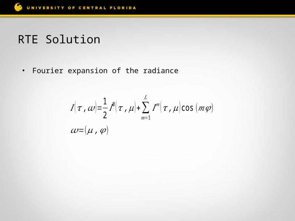
• Fourier expansion of the radiance
𝐼 (𝜏 ,𝜔 )=12𝐼 0 (𝜏 ,𝜇 )+ ∑
𝑚=1
𝐿
𝐼𝑚 (𝜏 ,𝜇) cos (𝑚𝜑 )
𝜔=(𝜇 ,𝜑 )
RTE Solution
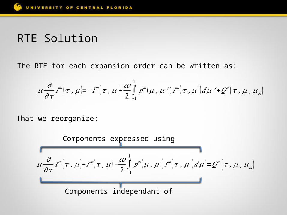
The RTE for each expansion order can be written as:
𝜇 𝜕𝜕𝜏
𝐼𝑚 (𝜏 ,𝜇)=− 𝐼𝑚 (𝜏 ,𝜇 )+𝜔2∫− 1
1
𝑝𝑚 (𝜇 ,𝜇 ′) 𝐼𝑚 (𝜏 ,𝜇′)𝑑𝜇 ′+𝑄𝑚 (𝜏 ,𝜇 ,𝜇𝑖𝑛)
That we reorganize:
𝜇 𝜕𝜕𝜏
𝐼𝑚 (𝜏 ,𝜇) +𝐼𝑚 (𝜏 ,𝜇)−𝜔2∫−1
1
𝑝𝑚 (𝜇 ,𝜇′ ) 𝐼𝑚 (𝜏 ,𝜇′ )𝑑𝜇′=𝑄𝑚 (𝜏 ,𝜇 ,𝜇𝑖𝑛 )
Components expressed using
Components independant of
RTE Solution
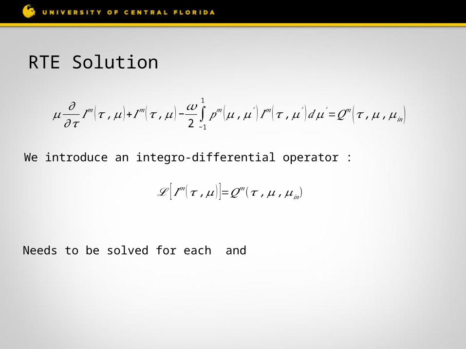
We introduce an integro-differential operator :
ℒ [ 𝐼𝑚 (𝜏 ,𝜇 ) ]=𝑄𝑚(𝜏 ,𝜇 ,𝜇𝑖𝑛)
Needs to be solved for each and
𝜇 𝜕𝜕𝜏
𝐼𝑚 (𝜏 ,𝜇) +𝐼𝑚 (𝜏 ,𝜇)−𝜔2∫−1
1
𝑝𝑚 (𝜇 ,𝜇′ ) 𝐼𝑚 (𝜏 ,𝜇′ )𝑑𝜇′=𝑄𝑚 (𝜏 ,𝜇 ,𝜇𝑖𝑛 )
RTE Solution
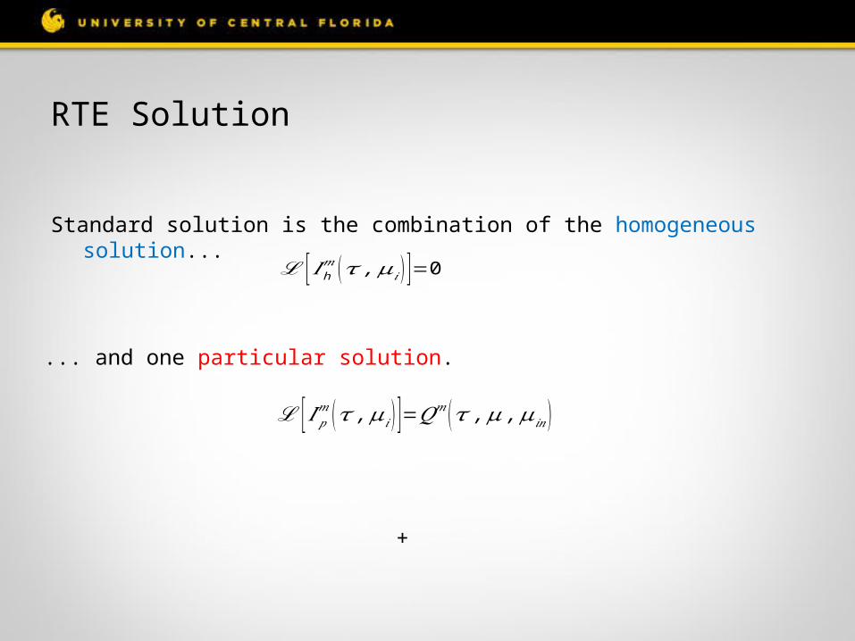
Standard solution is the combination of the homogeneous solution...
ℒ [ 𝐼 h𝑚 (𝜏 ,𝜇𝑖 ) ]=0
... and one particular solution.
ℒ [ 𝐼𝑝𝑚 (𝜏 ,𝜇𝑖 ) ]=𝑄𝑚 (𝜏 ,𝜇 ,𝜇𝑖𝑛 )
+
RTE Solution
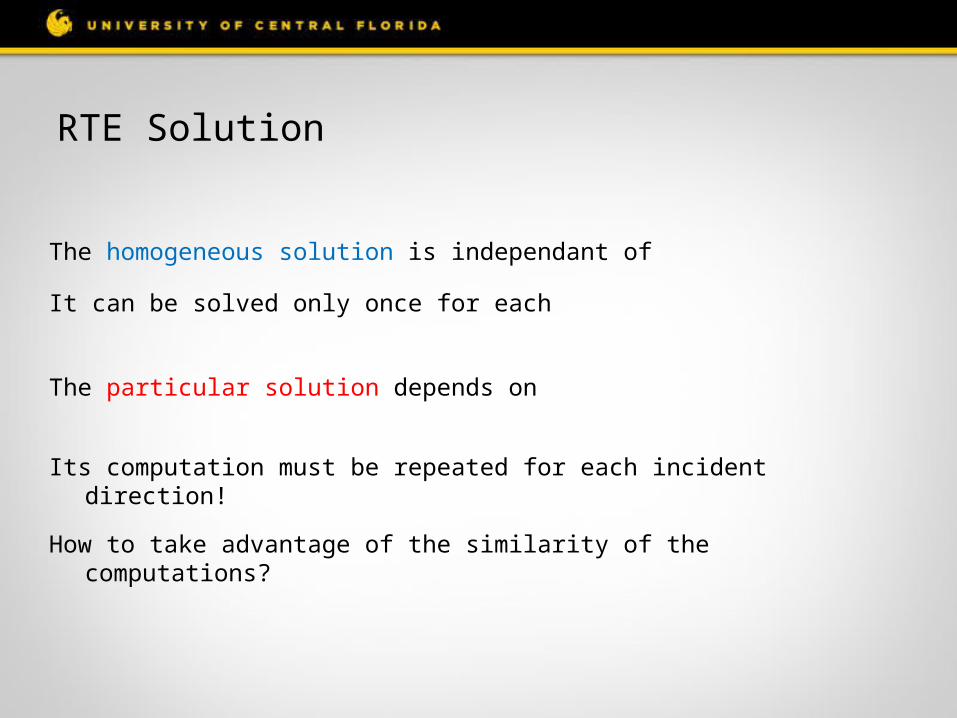
The homogeneous solution is independant of
The particular solution depends on
It can be solved only once for each
Its computation must be repeated for each incident direction!
How to take advantage of the similarity of the computations?
Green’s function solution
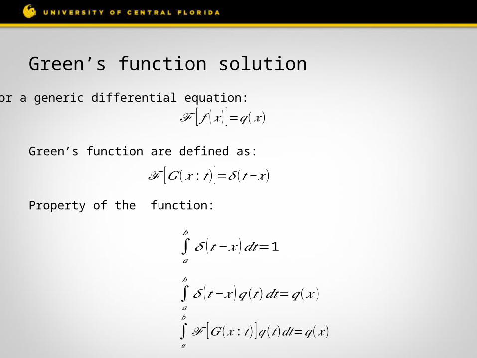
Green’s function are defined as:
ℱ [𝐺(𝑥 :𝑡)]=𝛿(𝑡−𝑥)
Property of the function:
∫𝑎
𝑏
𝛿 (𝑡−𝑥 ) 𝑑𝑡=1
ℱ [ 𝑓 (𝑥 ) ]=𝑞(𝑥 )
∫𝑎
𝑏
𝛿 (𝑡−𝑥 )𝑞(𝑡)𝑑𝑡=𝑞 (𝑥 )
For a generic differential equation:
∫𝑎
𝑏
ℱ [𝐺(𝑥 :𝑡) ]𝑞 (𝑡)𝑑𝑡=𝑞 (𝑥)
Green’s function solution
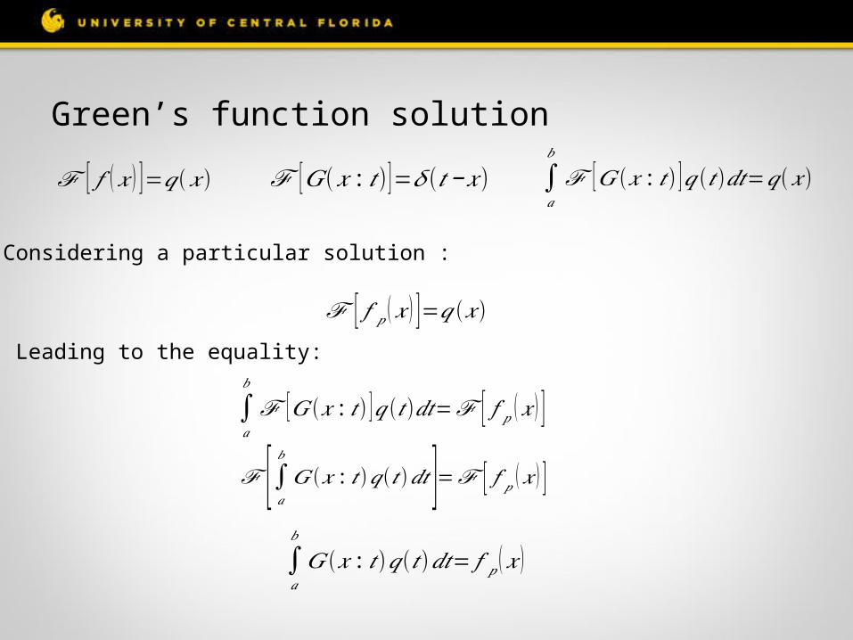
ℱ [ 𝑓 (𝑥 ) ]=𝑞(𝑥 )
ℱ [ 𝑓 𝑝 (𝑥 ) ]=𝑞(𝑥)
∫𝑎
𝑏
ℱ [𝐺(𝑥 :𝑡) ]𝑞 (𝑡)𝑑𝑡=ℱ [ 𝑓 𝑝 (𝑥 ) ]
ℱ [∫𝑎
𝑏
𝐺(𝑥 :𝑡)𝑞 (𝑡)𝑑𝑡 ]=ℱ [ 𝑓 𝑝 (𝑥 ) ]
ℱ [𝐺(𝑥 :𝑡)]=𝛿(𝑡−𝑥) ∫𝑎
𝑏
ℱ [𝐺(𝑥 :𝑡) ]𝑞 (𝑡)𝑑𝑡=𝑞 (𝑥)
Considering a particular solution :
Leading to the equality:
∫𝑎
𝑏
𝐺(𝑥 :𝑡)𝑞(𝑡 )𝑑𝑡= 𝑓 𝑝 (𝑥 )
Green’s function solution
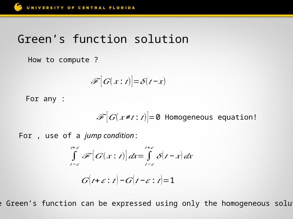
How to compute ?
ℱ [𝐺(𝑥 :𝑡)]=𝛿(𝑡−𝑥)
For any :
ℱ [𝐺(𝑥≠ 𝑡 :𝑡)]=0 Homogeneous equation!
For , use of a jump condition:
∫𝑡−𝜀
𝑡+𝜀
ℱ [𝐺(𝑥 :𝑡)]𝑑𝑥=∫𝑡−𝜀
𝑡+𝜀
𝛿 (𝑡− 𝑥 )𝑑𝑥
𝐺 (𝑡+𝜀 :𝑡 )−𝐺 (𝑡−𝜀 :𝑡 )=1
The Green’s function can be expressed using only the homogeneous solution
Back to the RTE
ℒ [ 𝐼𝑚 (𝜏 ,𝜇 ) ]=𝑄𝑚(𝜏 ,𝜇 ,𝜇𝑖𝑛)
𝜇 𝜕𝜕𝜏
𝐼𝑚 (𝜏 ,𝜇) +𝐼𝑚 (𝜏 ,𝜇)−𝜔2∫−1
1
𝑝𝑚 (𝜇 ,𝜇′ ) 𝐼𝑚 (𝜏 ,𝜇′ )𝑑𝜇′=𝑄𝑚 (𝜏 ,𝜇 ,𝜇𝑖𝑛 )
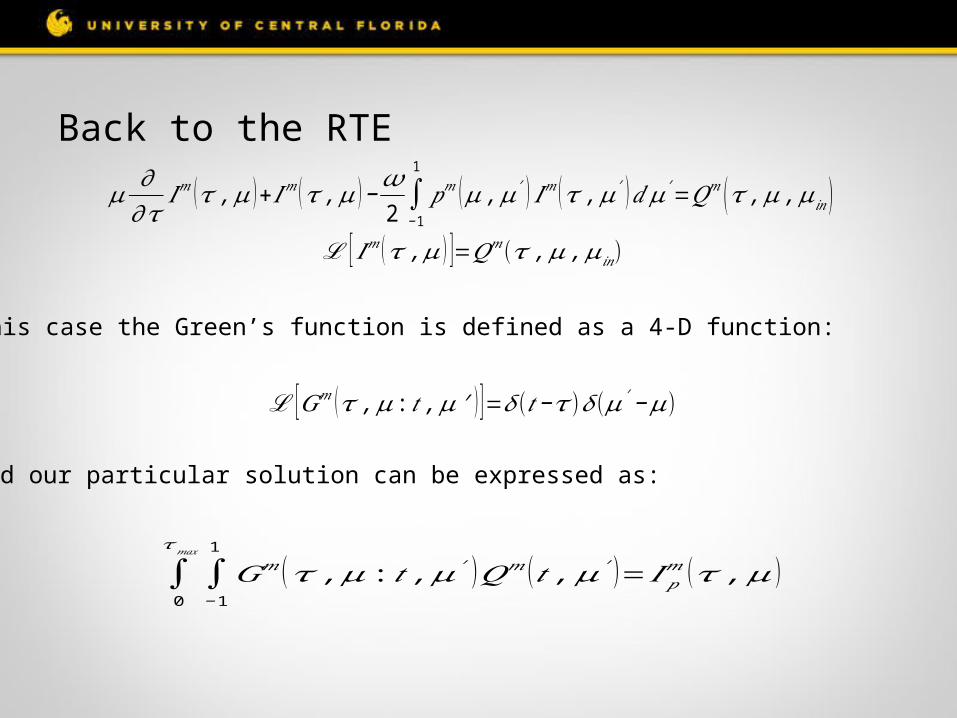
In this case the Green’s function is defined as a 4-D function:
ℒ [𝐺𝑚 (𝜏 ,𝜇 :𝑡 ,𝜇 ′ ) ]=𝛿(𝑡−𝜏)𝛿(𝜇′−𝜇)
And our particular solution can be expressed as:
∫0
𝜏𝑚𝑎𝑥
∫− 1
1
𝐺𝑚 (𝜏 ,𝜇 :𝑡 ,𝜇′ )𝑄𝑚 ( 𝑡 ,𝜇′ )=𝐼𝑝𝑚 (𝜏 ,𝜇)
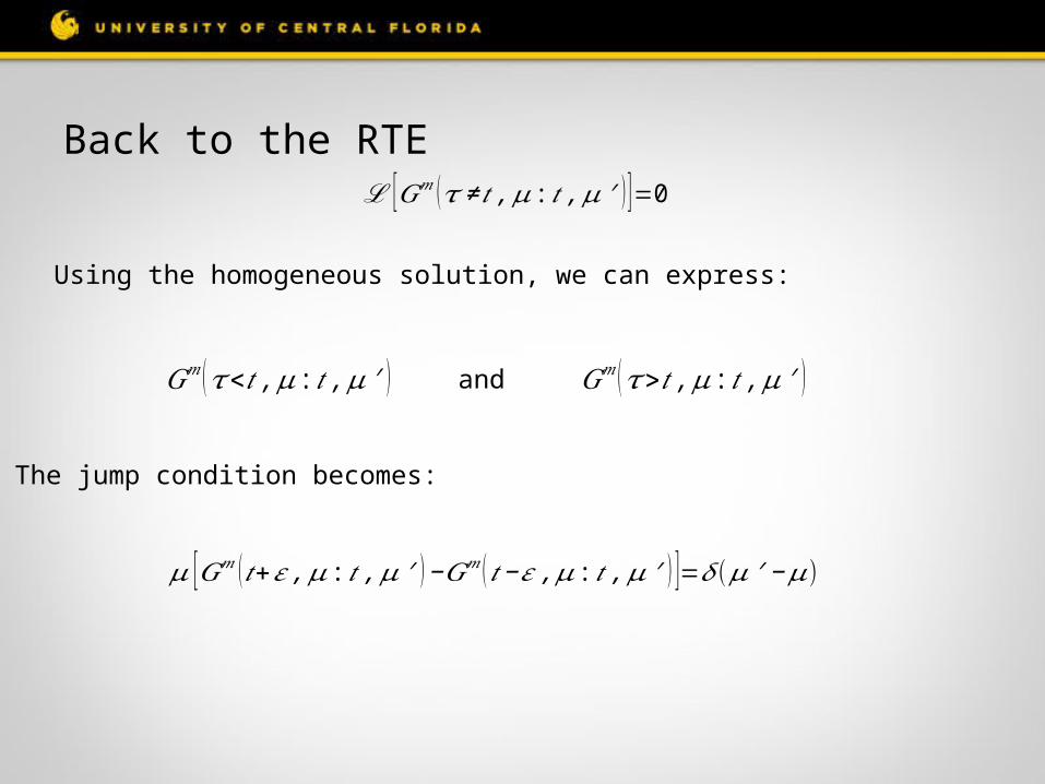
Back to the RTEℒ [𝐺𝑚 (𝜏 ≠ 𝑡 ,𝜇 :𝑡 ,𝜇 ′ ) ]=0
Using the homogeneous solution, we can express:
𝐺𝑚 (𝜏<𝑡 ,𝜇 :𝑡 ,𝜇 ′ ) 𝐺𝑚 (𝜏>𝑡 ,𝜇 :𝑡 ,𝜇 ′ )and
The jump condition becomes:
𝜇 [𝐺𝑚 (𝑡+𝜀 ,𝜇 :𝑡 ,𝜇 ′ )−𝐺𝑚 (𝑡−𝜀 ,𝜇 :𝑡 ,𝜇 ′ ) ]=𝛿(𝜇 ′ −𝜇)

RTE Solution
The homogeneous solution is independant of
The particular solution is now an integration of the Green’s function
It is solved only once
The Green’s function can be expressed using 𝐼 h𝑚 (𝜏 ,𝜇𝑖 )
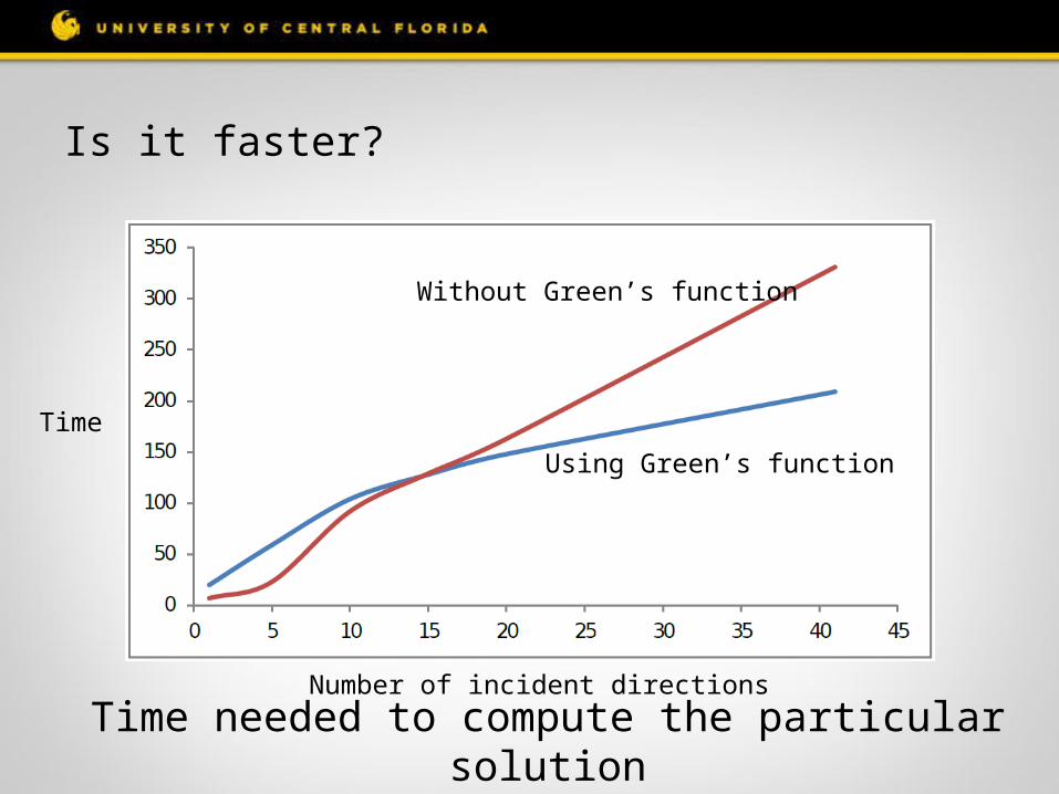
Is it faster?
Without Green’s function
Using Green’s function
Time
Number of incident directions
Time needed to compute the particular solution
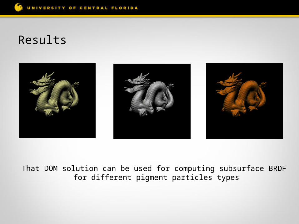
Results
That DOM solution can be used for computing subsurface BRDF for different pigment particles types
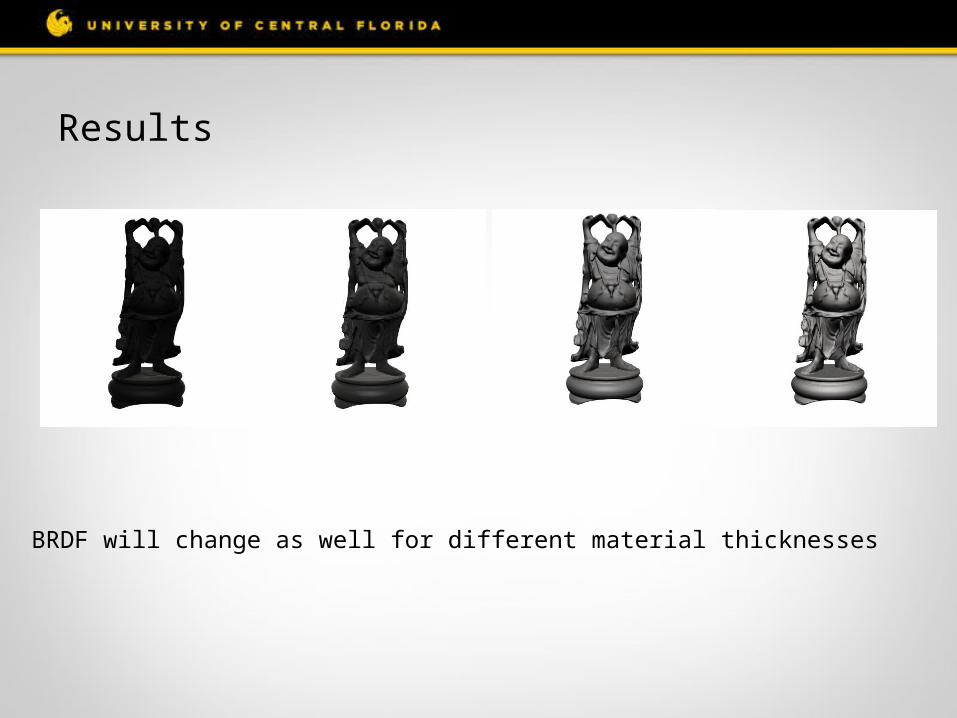
Results
BRDF will change as well for different material thicknesses
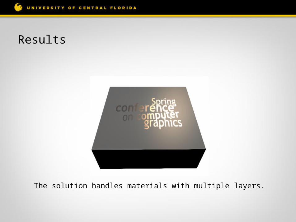
Results
The solution handles materials with multiple layers.
Thank you