Embed Size (px)
Citation preview
IEEE TRANSACTIONS ON VEHICULAR TECHNOLOGY 1
Ricean K-Factors in Narrow-Band Fixed WirelessChannels: Theory, Experiments, and
Statistical ModelsLarry J. Greenstein, Life Fellow, IEEE, Saeed S. Ghassemzadeh, Senior Member, IEEE,
Vinko Erceg, Fellow, IEEE, and David G. Michelson, Senior Member, IEEE
Abstract—Fixed wireless channels in suburban macrocells aresubject to fading due to scattering by moving objects such aswindblown trees and foliage in the environment. When, as is oftenthe case, the fading follows a Ricean distribution, the first-orderstatistics of fading are completely described by the correspondingaverage path gain and Ricean K-factor. Because such fading hasimportant implications for the design of both narrow-band andwideband multipoint communication systems that are deployed insuch environments, it must be well characterized. We conducted aset of 1.9-GHz experiments in suburban macrocell environmentsto generate a collective database from which we could construct asimple model for the probability distribution of K as experiencedby fixed wireless users. Specifically, we find K to be lognormal,with the median being a simple function of season, antenna height,antenna beamwidth, and distance and with a standard deviationof 8 dB. We also present plausible physical arguments to explainthese observations, elaborate on the variability of K with time,frequency, and location, and show the strong influence of windconditions on K .
Index Terms—Fading, fixed wireless channels, K-factors, multi-point communication, Ricean distribution.
I. INTRODUCTION
DURING the past decade, both common carriers and utili-ties have begun to deploy fixed wireless multipoint com-
munication systems in suburban environments. For commoncarriers, wideband multipoint communication systems providea method for delivering broadband voice and data to residenceswith greater flexibility than wired services. For utilities, narrow-band multipoint communication systems provide a convenientand independent method for controlling or monitoring theinfrastructure, including utility meters located on customerpremises. In the past, most narrow-band fixed wireless links
Manuscript received June 26, 2008; revised December 18, 2008. The reviewof this paper was coordinated by Dr. K. T. Wong.
L. J. Greenstein is with the Wireless Information Network Laboratory,Rutgers University, North Brunswick, NJ 08902 USA (e-mail: [email protected]).
S. S. Ghassemzadeh is with the Communication Technology ResearchDepartment, AT&T Labs-Research, Florham Park, NJ 07932 USA (e-mail:[email protected]).
V. Erceg is with the Broadcom Corporation, San Diego, CA 92128 USA(e-mail: [email protected]).
D. G. Michelson is with the Radio Science Laboratory, Department of Elec-trical and Computer Engineering, University of British Columbia, Vancouver,BC V6T 1Z4, Canada (e-mail: [email protected]).
Color versions of one or more of the figures in this paper are available onlineat http://ieeexplore.ieee.org.
Digital Object Identifier 10.1109/TVT.2009.2018549
were deployed in frequency bands below 900 MHz. In responseto increasing demand, both the Federal Communication Com-mission and Industry Canada have recently allocated severalnew bands between 1.4 and 2.3 GHz to such applications. Be-cause fading on fixed wireless links has important implicationsfor the design of both narrow-band and wideband multipointcommunication systems, it must be well characterized. Narrow-band fading models apply to both narrow-band signals and in-dividual carriers or pilot tones in orthogonal frequency-divisionmultiplexing systems such as those based upon the IEEE 802.16standard. Ideally, such models will capture not just the statisticsof fading but their dependence upon the type and density ofscatterers in the environment as well.
The complex path gain of any radio channel can quitegenerally be represented as having a fixed component plus afluctuating (or scatter) component. The former might be dueto a line-of-sight path between the transmitter and the receiver;the latter is usually due to echoes from multiple local scatterers,which causes variations in space and frequency of the summedmultipath rays. The spatial variation is translated into a timevariation when either end of the link is in motion. In the case offixed wireless channels, time variation is a result of scatterersin motion.
If the scatter component has a complex Gaussian distribution,as it does in the central limit (many echoes of comparablestrength), the time-varying magnitude of the complex gain willhave a Ricean distribution. The key parameter of this distribu-tion is the Ricean K-Factor (or just K), which is the power ratioof the fixed and scatter components [1]–[3]. It is a measure ofthe severity of fading. The case K = 0 (no fixed component)corresponds to the most severe fading, and in this limiting case,the gain magnitude is said to be Rayleigh distributed. From theearliest days, most analyses of mobile cellular systems, e.g., [4],have assumed Rayleigh fading because it is both conservativeand quite prevalent.
The case of fixed wireless paths, e.g., for wireless multipointcommunication systems, is different. Here, there can still bemultipath echoes, and the complex sums of received wavesstill vary over space and frequency. However, with both endsof the link fixed, there will be—to first order—no temporalvariations. What alters this first-order picture is the slow motionof scatterers along the path, e.g., pedestrians, vehicles, andwind-blown leaves and foliage. As a result, the path gain atany given frequency will exhibit slow temporal variations as
0018-9545/$25.00 © 2009 IEEE

2 IEEE TRANSACTIONS ON VEHICULAR TECHNOLOGY
the relative phases of arriving echoes change. Because theseperturbations are often slight, the condition of a dominant fixedcomponent plus a smaller fluctuating component takes on ahigher probability than that for mobile links. Furthermore, sincetemporal perturbations can occur on many scatter paths, theconvergence of their sum to a complex Gaussian process isplausible. Therefore, we can expect a Ricean distribution forthe gain magnitude, with a higher K-factor, in general, thanthat for mobile cellular channels.
During the past decade, numerous studies have aimed toreveal various aspects of the manner in which fixed wirelesschannels fade on non-line-of-sight paths typical of those en-countered in urban and suburban environments [5]–[12]. Oneset of researchers has focused on determining the manner inwhich wind blowing through foliage affects the depth of fadingon fixed links, e.g., [6]–[9], while another has focused on sce-narios in which relatively little foliage is present but scatteringfrom vehicular traffic presents a significant impairment, e.g.,[10]–[12].
In this paper, we focus on the development of statisticalmodels that capture the manner in which fading on fixedwireless channels in suburban macrocell environments dependsupon the local environment, the season (leaves or no leaves),the distance between the base and the remote terminal, andthe height and beamwidth of the terminal antenna. We do sousing an extensive body of data collected during four distinctexperiments. Our earlier findings were presented in [13] andwere ultimately adopted by IEEE 802.16 [14]. Here, we fill inthe essential detail concerning the measurement campaigns andpresent plausible physical arguments to explain our observa-tions. Furthermore, we demonstrate that the variability of thechannel about the median can be divided into a componentdue to variation at a fixed location and another due to variationbetween locations. Finally, we present what we believe are thefirst observations of simultaneous fading events on differentlinks within the same suburban macrocell.
In Section II, we review a method for computing K fromtime records of path gain magnitude that is particularly fastand robust and therefore suited to high-volume data reductions.We show that it is also highly accurate. In Section III, wedescribe several experiments that were conducted at 1.9 GHz tomeasure path gains on fixed wireless links. The data from theseexperiments were used to compute K-factors for narrow-bandchannels. In Section IV, we show how the computed resultswere used to model the statistics of K as a function of variousparameters. We also examine such issues as the variability ofK with time, frequency, and location and the influence of windconditions on K. Section V concludes the paper.
II. ESTIMATION OF RICEAN K-FACTOR
A. Background
Our practical objective is to model narrow-band fading bymeans of a Ricean distribution over the duration of a fixed wire-less connection. We assume that the duration of a connection isin the 5–15-min range, and we will compute K for finite timeintervals of that order. Later, we will show how K can varywith the time segment and with frequency. We will also show
that the statistical model for K is very similar for 5- and 15-minintervals.
B. Formulation
We characterize the complex path gain of the narrow-bandwireless channel by a frequency-flat time-varying response
g(t) = V + v(t) (1)
where V is a fixed complex value, and v(t) is a complex zero-mean random time fluctuation caused by vehicular motion,wind-blown foliage, etc., with variance σ2. This descriptionapplies to a particular frequency and time segment. Both V andσ2 may change from one time–frequency segment to another.
We assume that the quantity actually measured is the receivednarrow-band power, which, suitably normalized, yields theinstantaneous power gain
G(t) = |g(t)|2 . (2)
Various methods have been reported to estimate K usingmoments calculated from time series such as (2), e.g.,[15]–[17].
We can relate K to two moments that can be estimated fromthe data record for G(t). The first moment Gm is the averagepower gain; its true value (as distinct from the estimate
Gm =N∑
i=1
Gi
n(3)
computed from finite data) is shown in [15] to be
Gm = |V |2 + σ2. (4)
The second moment Gv is the RMS fluctuation of G aboutGm. The true value of this moment (as distinct from theestimate
Gv =
√√√√ 1N
N∑i=1
(Gi − Gm)2 (5)
calculated from finite data) is shown in [15] to be
Gm =√
σ4 + 2|V |2σ2. (6)
In each of (4) and (6), the left-hand side can be estimatedfrom the data, and the right-hand side is a function of the twointermediate quantities we seek. Combining these equations,we can solve for |V |2 and σ2, yielding
|V |2 =√
G2m − G2
v (7)
σ2 = Gm −√
G2m − G2
v. (8)
Finally, K is obtained by substituting these two values into
K = |V |2/σ2. (9)
Note that σ2 as defined here is twice the RF power of thefluctuating term, which is why the customary factor of two

GREENSTEIN et al.: RICEAN K-FACTORS IN NARROW-BAND FIXED WIRELESS CHANNELS 3
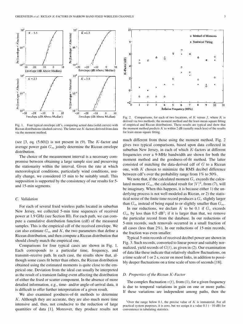
Fig. 1. Four typical envelope cdf’s, comparing actual data (solid curves) withRicean distributions (dashed curves). The latter use K-factors derived from datavia the moment method.
(see [3, eq. (5.60)]) is not present in (9). The K-factor andaverage power gain Gm jointly determine the Ricean envelopedistribution.
The choice of the measurement interval is a necessary com-promise between obtaining a large sample size and preservingthe stationarity within the interval. Given the rate at whichmeteorological conditions, particularly wind conditions, usu-ally change, we considered 15 min to be suitably small. Thissupposition is supported by the consistency of our results for 5-and 15-min segments.
C. Validation
For each of several fixed wireless paths located in suburbanNew Jersey, we collected 5-min time sequences of receivedpower at 1.9 GHz (see Section III). For each path, we can com-pute a cumulative distribution function (cdf) of the measuredsamples. This is the empirical cdf of the received envelope. Wecan also estimate Gm and K, the two parameters that define aRicean distribution, and then compute a Ricean distribution thatshould closely match the empirical one.
Comparisons for four typical cases are shown in Fig. 1.Each corresponds to a particular time, frequency, andtransmit–receive path. In each case, the results show that, al-though some cases fit better than others, the Ricean distributionobtained using the estimated moments is quite close to the em-pirical one. Deviation from the ideal can usually be interpretedas the result of a transient fading event affecting the distributionof either the fixed or scatter component. In the absence of moredetailed information, e.g., time- and/or angle-of-arrival data, itis difficult to offer further interpretation of a given result.
We also examined goodness-of-fit methods to determineK. Although they are accurate, they are also much more timeintensive and, thus, not conducive to the reduction of largequantities of data [1]. Moreover, they produce results not
Fig. 2. Comparisons, for each of two locations, of K versus f , where K isderived via two methods: the moment method and the least-mean-square fittingof empirical and Ricean distributions. These results are typical and show thatthe moment method predicts K to within 2 dB (usually much less) of the resultsfor least-mean-square fitting.
much different from those using the moment method. Fig. 2gives two typical comparisons, based upon data collected insuburban New Jersey, in each of which K-factors at differentfrequencies over a 9-MHz bandwidth are shown for both themoment method and the goodness-of-fit method. The latterconsisted of matching the data-derived cdf of G to a Riceanone, with K chosen to minimize the RMS decibel differencebetween cdf’s over the probability range from 1% to 50%.
We note that, if the calculated moment Gv exceeds the calcu-lated moment Gm, the calculated result for |V |2, from (7), willbe imaginary. When this happens, it is because either 1) the un-derlying process is not well modeled as Ricean, or 2) the statis-tical noise of the finite time record produces a Gv slightly largerthan Gm instead of being equal to or slightly smaller than Gm.
In our reductions, we declare K to be 0.1 if Gv exceedsGm by less than 0.5 dB1; if it is larger than that, we removethe particular record from the database. In our reductions of5-min records, such removals occurred in a small fraction ofall cases (less than 2%). In our reductions of 15-min records,the fraction was even smaller.
Typical 5-min records of received decibel power are shown inFig. 3. Such records, converted to linear power and suitably nor-malized, yield records of G(t), as given in (2). Our examinationof data like these indicate that relatively shallow fluctuations, ona time scale of 1 or 2 s, occur on most links, in addition to possi-bly deeper fluctuations on a time scale of tens of seconds [18].
D. Properties of the Ricean K-Factor
The complex fluctuation v(t), from (1), for a given frequencyis due to temporal variations in gain on one or more paths.If these variations are independent among paths, then the
1Over the range below 0.1, the precise value of K is immaterial. For allpractical system purposes, it is zero, but we assign it a value 0.1 (−10 dB) forconvenience in tabulating statistics.

4 IEEE TRANSACTIONS ON VEHICULAR TECHNOLOGY
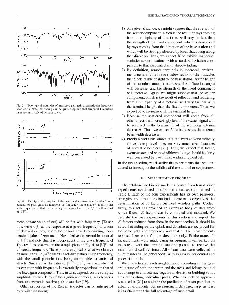
Fig. 3. Two typical examples of measured path gain at a particular frequencyover 280 s. Note that fading can be quite deep and that temporal fluctuationrates are on a scale of hertz or lower.
Fig. 4. Two typical examples of the fixed and mean-square “scatter” com-ponents of path gain, as functions of frequency. Note that σ2 is fairly flatwith frequency, so that the frequency variation of K = |V |2/σ2 follows thatof |V |2.
mean-square value of v(t) will be flat with frequency. [To seethis, write v(t) as the response at a given frequency to a sumof delayed echoes, where the echoes have time-varying inde-pendent gains of zero mean. Next, derive the ensemble mean of|v(t)|2, and note that it is independent of the given frequency.]This result is observed in the sample plots, in Fig. 4, of |V |2 andσ2 versus frequency. These plots are typical of what we observeon most links, i.e., σ2 exhibits a relative flatness with frequency,with the small perturbations being attributable to statisticaleffects. Since K is the ratio of |V |2 to σ2, we conclude thatits variation with frequency is essentially proportional to that ofthe fixed gain component. This, in turn, depends on the complexamplitude versus delay of the significant echoes, which variesfrom one transmit–receive path to another [19].
Other properties of the Ricean K-factor can be anticipatedby similar reasoning.
1) At a given distance, we might suppose that the strength ofthe scatter component, which is the result of rays comingfrom a multiplicity of directions, will vary far less thanthe strength of the fixed component, which is dominatedby rays coming from the direction of the base station andwhich will be strongly affected by local shadowing alongthat direction. Thus, we expect K to exhibit lognormalstatistics across locations, with a standard deviation com-parable to that associated with shadow fading.
2) By definition, remote terminals in macrocell environ-ments generally lie in the shadow region of the obstaclesthat block its line of sight to the base station. As the heightof the terminal antenna increases, the diffraction anglewill decrease, and the strength of the fixed componentwill increase. Again, we might suppose that the scattercomponent, which is the result of reflection and scatteringfrom a multiplicity of directions, will vary far less withthe terminal height than the fixed component. Thus, weexpect K to increase with the terminal height.
3) Because the scattered component will come from allother directions, increasingly less of the scatter signal willbe received as the beamwidth of the receiving antennadecreases. Thus, we expect K to increase as the antennabeamwidth decreases.
4) Previous work has shown that the average wind velocityabove treetop level does not vary much over distancesof several kilometers [20]. Thus, we expect that fadingevents associated with windblown foliage should be fairlywell correlated between links within a typical cell.
In the next section, we describe the experiments that we con-ducted to investigate the validity of these and other conjectures.
III. MEASUREMENT PROGRAM
The database used in our modeling comes from four distinctexperiments conducted in suburban areas, as summarized inTable I. Each of the four experiments has its own purposes,strengths, and limitations but had, as one of its objectives, thedetermination of K-factors on fixed wireless paths. Collec-tively, this set has provided an extensive body of data fromwhich Ricean K-factors can be computed and modeled. Wedescribe the four experiments in this section and report theK-factors reduced from them in the next section. It should benoted that fading on the uplink and downlink are reciprocal forthe same path and frequency and that all the measurementsreported here were for the downlink only. Furthermore, allmeasurements were made using an equipment van parked onthe street, with the terminal antenna pointed to receive themaximum downlink signal. All of our data were collected inquiet residential neighborhoods with minimum residential andpedestrian traffic.
We characterized each neighborhood according to the gen-eral nature of both the terrain and the trees and foliage but didnot attempt to characterize vegetation density or building-to-lotarea ratios along individual paths. Whereas such an approachwas used in [21] to assist in the prediction of mean path loss inurban environments, our measurement database, large as it is,is insufficient to take full advantage of such detail.

GREENSTEIN et al.: RICEAN K-FACTORS IN NARROW-BAND FIXED WIRELESS CHANNELS 5
TABLE ISUMMARY OF THE FOUR EXPERIMENTS
A. Experiment 1: Short-Term Measurements in New Jersey
Downlink measurements were made for three transmit sitesin northern and central New Jersey. For each site, data were col-lected at 33 or more downlink locations during summer (treesin full bloom), and repeat measurements were made at half ormore of these locations during winter (trees bare). Distancesranged (more or less uniformly) from 0.5 to 9 km. This was themajor experiment in our study, and so, we summarize a numberof its features in Table II.
The transmit sites were located in the residential communi-ties of Holmdel, Whippany, and Clark. Each site overlookeda terrain consisting of rolling hills with moderate to heavy treedensities and dwellings of one or two stories. Furthermore, eachsite used a panel-type transmitting antenna with elevation andazimuth beamwidths of 16◦ and 65◦, respectively. The antennawas fed by a 10-MHz swept frequency generator centered at1985 MHz.
For each downlink location (i.e., receive terminal site) foreach of two antennas at each of two heights (3 and 10 m),the data record consists of 700 “snapshots” of received powerversus frequency. The receiver was a swept frequency spectrumanalyzer equipped with a low noise amplifier to increase itssensitivity; its sweep was synchronized to that of the transmit-ter using the 1-pulse-per-second signal from a GPS receiver.The unit was operated in sample detection mode to enhanceits ability to characterize the first-order statistics of randomsignals. A local controller handled the configuration, operation,and data acquisition. The “snapshots” for each antenna/heightcombination are spaced by 0.4 s, for a total time span of nearly5 min, and each consists of 90 samples, spaced by 100 kHz,for a frequency span of 9 MHz. In the data processing, thepower samples, which were recorded in decibels of the mea-sured power referenced to 1 mW (dBm), were calibrated andconverted to linear path gain.

6 IEEE TRANSACTIONS ON VEHICULAR TECHNOLOGY
TABLE IIFEATURES OF EXPERIMENT 1
B. Experiment 2: Short-Term Measurements in Illinoisand Washington
During the spring and summer, measurements were made inthe vicinity of a transmit site in Washington (Redmond, nearSeattle) and from two transmit sites in Illinois (Bellwood andNaperville, near Chicago). The number of downlink locationswas more than 100 for each transmit site at distances rangingfrom 0.4 to 2.2 km.
All three transmit sites were in suburban/residential envi-ronments. The Redmond site overlooked a hilly terrain withheavy tree cover. The Bellwood and Naperville sites overlookedan extremely flat terrain with high and low tree densities,respectively. The measurement data were collected using acontinuous-wave (CW) transmitter and multichannel narrow-band measurement receiver manufactured by Grayson Elec-tronics. The amplitude resolution was 1 dB, which was deemedto be adequate for the purpose of determining K.
Two antennas were used at each downlink location: onedirectional and one omnidirectional. They were used to simul-taneously make measurements and were both mounted at aheight of 3 m. No measurements were made in winter. Eachmeasurement consisted of recording the received signal powerat a rate of 400 samples/s for 5 min.
C. Experiment 3: Long-Term Measurements in New Jersey
Long-term measurements (record lengths of up to 24 h) weremade from two transmit sites in northern New Jersey: onein Iselin and one in Whippany. The Whippany site was thesame as the one used in Experiment 1. The Iselin site used asimilar transmit antenna, at a height of 15 m, and overlooked aresidential area similar to that in Whippany. The total numberof downlink locations processed for these two sites was 16, withdistances ranging from 0.5 to 3.1 km.
The measurement approach was similar to that for Experi-ment 1: The received power was recorded at 100 frequenciesover 10 MHz centered on 1985 MHz. The three main differ-ences were 1) the reception was on the two branches of a slant-
Fig. 5. CDFs of the K-factor for an antenna beamwidth of 30◦. These resultsare for New Jersey locations measured in Experiment 1.
45◦ dual-polarized antenna with an azimuth beamwidth of 32◦,2) data were recorded for continuous intervals ranging from 11to 24 h, and 3) the wind speed was continuously measured andrecorded at both ends of the path.
In the data reductions, only the central 6 MHz of data wereprocessed (60 frequencies), and the long time records wereparsed into 15-min segments. Thus, a 24-h recording produceda 96 × 60 matrix of time–frequency segments, and K wascomputed for each one. This permitted us to obtain K for timesegments longer than the original 5-min samples as well as toexamine slow variations in K over the course of a day. Thedecision to limit the number of frequencies processed was abusiness decision that does not materially affect the results.Indeed, the fact that single-carrier and multicarrier results withdifferent parameters yield consistent results gives us greaterconfidence in the generality of our findings.
D. Experiment 4: Long-Term Measurements in Illinois
Long-term measurements were made from two transmit sitesin Illinois, i.e., the same Bellwood and Naperville sites used in
GREENSTEIN et al.: RICEAN K-FACTORS IN NARROW-BAND FIXED WIRELESS CHANNELS 7
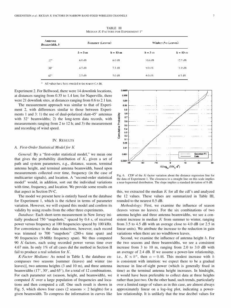
TABLE IIIMEDIAN K-FACTORS FOR EXPERIMENT 1∗
Experiment 2. For Bellwood, there were 14 downlink locations,at distances ranging from 0.35 to 1.4 km; for Naperville, therewere 21 downlink sites, at distances ranging from 0.6 to 2.1 km.
The measurement approach was similar to that of Experi-ment 2, with differences similar to those between Experi-ments 1 and 3: 1) the use of dual-polarized slant-45◦ antennaswith 32◦ beamwidths; 2) the long-term data records, withmeasurements ranging from 2 to 12 h; and 3) the measurementand recording of wind speed.
IV. RESULTS
A. First-Order Statistical Model for K
General: By a “first-order statistical model,” we mean onethat gives the probability distribution of K, given a set ofpath and system parameters, e.g., distance, season, terminalantenna height, and terminal antenna beamwidth, based uponmeasurements collected over time, frequency (in the case ofmulticarrier signals), and location. A “second-order statisticalmodel” would, in addition, sort out the individual variationswith time, frequency, and location. We provide some results onthat aspect in Section IV-C.
The model we present here is entirely based on the databasefor Experiment 1, which is the richest in terms of parametervariation. However, we will expand this model and confirm itsvalidity by using results from the other three experiments.
Database: Each short-term measurement in New Jersey ini-tially produced 750 “snapshots,” spaced by 0.4 s, of receivedpower versus frequency at 100 frequencies spaced by 100 kHz.For convenience in the data reductions, however, each recordwas trimmed to 700 “snapshots” (280-s time span) and90 frequencies (9-MHz frequency span). We thus computed90 K-factors, each using recorded power versus time over4.67 min. In only 1% of all cases did the method in Section IIfail to produce a real solution for K.
K-Factor Medians: As noted in Table I, the database en-compasses two seasons [summer (leaves) and winter (noleaves)], two antenna heights (3 and 10 m), and three antennabeamwidths (17◦, 30◦, and 65◦), for a total of 12 combinations.For each parameter set (season, height, and beamwidth), wecomputed K over a large population of frequencies and loca-tions and then computed a cdf. One such result is shown inFig. 5, which shows four cases (2 seasons × 2 heights) for agiven beamwidth. To compress the information in curves like
Fig. 6. CDF of the K-factor variation about the distance regression line forthe data of Experiment 1. The closeness to a straight line on this scale impliesa near-lognormal distribution. The slope implies a standard deviation of 8 dB.
this, we extracted the median K for all the cdf’s and analyzedthe 12 values. These values are summarized in Table III,rounded to the nearest 0.5 dB.
Methodology: First, we examine the influence of season(leaves versus no leaves). For the six combinations of twoantenna heights and three antenna beamwidths, we see a con-sistent increase in median K from summer to winter, rangingfrom 3.5 to 4.5 dB with an average close to 4.0 dB (or 2.5 inlinear units). We attribute the increase to the reduction in gainvariations when there are no windblown leaves.
Second, we examine the influence of antenna height h. Forthe two seasons and three beamwidths, we see a consistentincrease from 3 to 10 m, ranging from 2.0 to 3.0 dB withan average of 2.4 dB. If we assume a power-law relationship,i.e., K ∝ hα, then α = 0.46. This modest increase with his consistent with intuition: we expect there to be a gradualincrease in line-of-sight power (which is generally fixed intime) as the terminal antenna height increases. In hindsight,it would have been preferable to collect data at three heightsrather than just two. On the other hand, such trends, particularlyover a limited range of values as in this case, are almost alwaysapproximately linear on a log–log plot, indicating a power-law relationship. It is unlikely that the true decibel values for
8 IEEE TRANSACTIONS ON VEHICULAR TECHNOLOGY
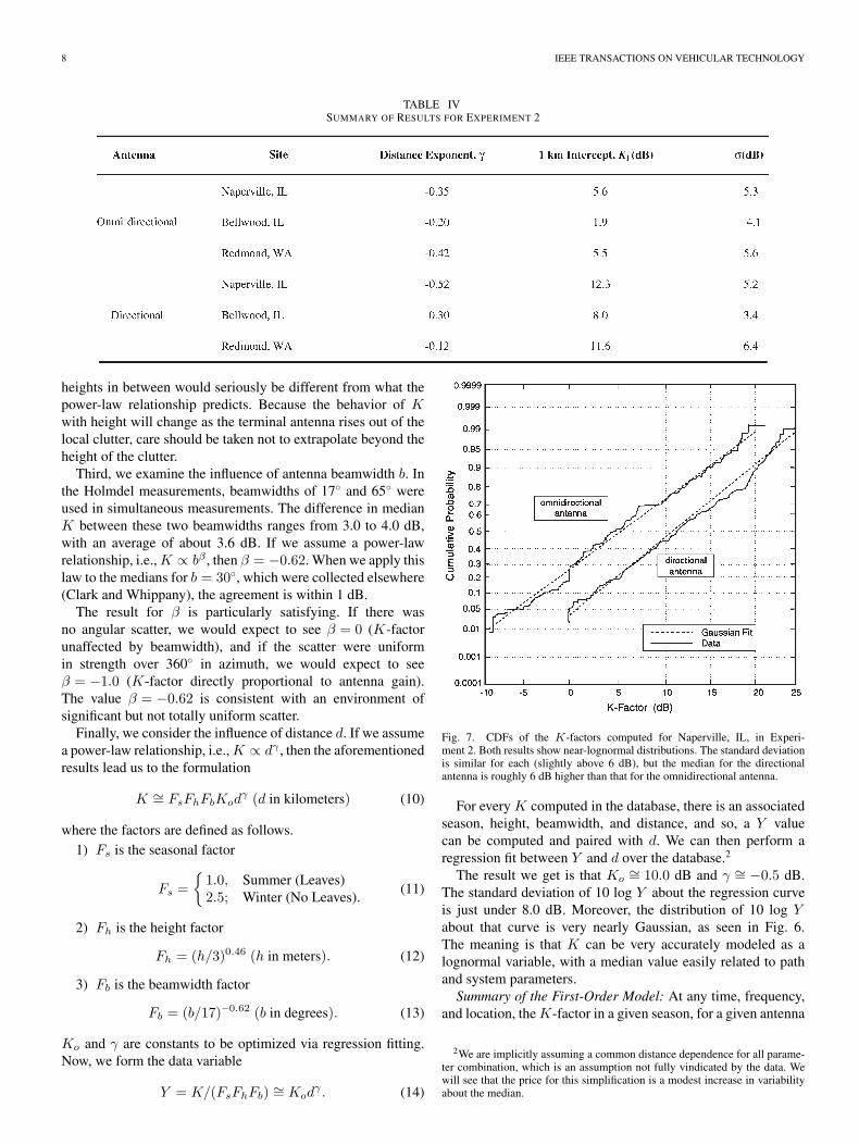
TABLE IVSUMMARY OF RESULTS FOR EXPERIMENT 2
heights in between would seriously be different from what thepower-law relationship predicts. Because the behavior of Kwith height will change as the terminal antenna rises out of thelocal clutter, care should be taken not to extrapolate beyond theheight of the clutter.
Third, we examine the influence of antenna beamwidth b. Inthe Holmdel measurements, beamwidths of 17◦ and 65◦ wereused in simultaneous measurements. The difference in medianK between these two beamwidths ranges from 3.0 to 4.0 dB,with an average of about 3.6 dB. If we assume a power-lawrelationship, i.e., K ∝ bβ , then β = −0.62. When we apply thislaw to the medians for b = 30◦, which were collected elsewhere(Clark and Whippany), the agreement is within 1 dB.
The result for β is particularly satisfying. If there wasno angular scatter, we would expect to see β = 0 (K-factorunaffected by beamwidth), and if the scatter were uniformin strength over 360◦ in azimuth, we would expect to seeβ = −1.0 (K-factor directly proportional to antenna gain).The value β = −0.62 is consistent with an environment ofsignificant but not totally uniform scatter.
Finally, we consider the influence of distance d. If we assumea power-law relationship, i.e., K ∝ dγ , then the aforementionedresults lead us to the formulation
K ∼= FsFhFbKodγ (d in kilometers) (10)
where the factors are defined as follows.1) Fs is the seasonal factor
Fs ={
1.0, Summer (Leaves)2.5; Winter (No Leaves).
(11)
2) Fh is the height factor
Fh = (h/3)0.46 (h in meters). (12)
3) Fb is the beamwidth factor
Fb = (b/17)−0.62 (b in degrees). (13)
Ko and γ are constants to be optimized via regression fitting.Now, we form the data variable
Y = K/(FsFhFb) ∼= Kodγ . (14)
Fig. 7. CDFs of the K-factors computed for Naperville, IL, in Experi-ment 2. Both results show near-lognormal distributions. The standard deviationis similar for each (slightly above 6 dB), but the median for the directionalantenna is roughly 6 dB higher than that for the omnidirectional antenna.
For every K computed in the database, there is an associatedseason, height, beamwidth, and distance, and so, a Y valuecan be computed and paired with d. We can then perform aregression fit between Y and d over the database.2
The result we get is that Ko∼= 10.0 dB and γ ∼= −0.5 dB.
The standard deviation of 10 log Y about the regression curveis just under 8.0 dB. Moreover, the distribution of 10 log Yabout that curve is very nearly Gaussian, as seen in Fig. 6.The meaning is that K can be very accurately modeled as alognormal variable, with a median value easily related to pathand system parameters.
Summary of the First-Order Model: At any time, frequency,and location, the K-factor in a given season, for a given antenna
2We are implicitly assuming a common distance dependence for all parame-ter combination, which is an assumption not fully vindicated by the data. Wewill see that the price for this simplification is a modest increase in variabilityabout the median.

GREENSTEIN et al.: RICEAN K-FACTORS IN NARROW-BAND FIXED WIRELESS CHANNELS 9
TABLE VSUMMARY OF RESULTS FOR EXPERIMENT 4
height, antenna beamwidth, and distance, can be described asfollows in a suburban New Jersey type of terrain:
K = K1dγu (15)
where K1 is the 1-km intercept
K1 = Fs · Fh · Fb · Ko (16)
Ko∼= 10.0 dB; γ ∼= −0.5; Fs, Fh, and Fb are given by
(9)–(11); and u is a lognormal variate, whose decibel value iszero mean with a standard deviation σ of 8.0 dB.
We observe that, for each of the 12 parameter sets identifiedearlier, the standard deviation about the decibel median for thatset was about 7 dB, or a bit more. The increase of less than1 dB in σ is mostly due to simplifications in modeling themedian, including assuming a common distance dependencefor all parameter sets. This small degree of added variabilityis a minor price for obtaining a simple and user-friendly model.
B. Consistency Checks
The reduced results from Experiment 2 are summarizedin Table IV. In computing K via (1)–(9), the percentage ofdata removed because K was not real was 0%, 1%, and 2%for Redmond, Naperville, and Bellwood, respectively, with nodifference between omnidirectional and directional antennas.We make the following observations.
1) The main difference between the terrains in Bellwoodand Naperville is tree density (high in Bellwood andlow in Naperville). The roughly 4-dB higher values forK1 in Naperville (3.7 and 4.3 dB for omnidirectionaland directional antennas, respectively) match the seasonaldifference for New Jersey (leaves versus no leaves).
2) The higher values of K1 for the directional antennasclosely follow the beamwidth dependence given by (13),which predicts a 5.6-dB increase for the 45◦ beamwidthused in Illinois and a 6.7-dB increase for the 30◦
beamwidth used in Washington. The agreements (within1 dB) are exceptionally good, particularly since (13) wasempirically derived for beamwidths of 65◦ and below.
3) The values of K1 for Bellwood and Naperville (takingproper account of the beamwidth and season) are within0.5 dB of the values predicted by the first-order model.
4) The numerical values for γ and σ in Table IV are con-sistent with those for the first-order model. The distanceexponent is smaller in some cases, and so is the standarddeviation. However, the data volume for Experiment 2 isnot large enough for these differences to be statisticallysignificant. What the tabulations show that is significantis that σ does not change with antenna beamwidth, inagreement with the first-order model.
5) The cdf’s of K in Illinois and Washington show the samelognormal character predicted by the first-order model.For example, Fig. 7 shows cdf’s of K, for both antennatypes, in Bellwood.
Now, moving to Experiment 3, we present a result that showsa remarkable consistency with the first-order model: Over60 frequencies and up to 96 time segments at 16 locations,K was found to be essentially lognormal, with a median andstandard deviation of 8.5 and 7.1 dB, respectively. Since thesedata were for distances uniformly clustered between 0.5 and2.0 km, the median closely corresponds to the 1-km interceptof the model, i.e., K1 in (16). For the conditions summer,h = 3 m, and b = 32◦, the model predicts K1 to be 8.3 dB.Furthermore, the 7.1-dB standard deviation is close to the8.0-dB model value, which is slightly elevated due to modelingapproximations.
Note that Experiments 1 and 3 were conducted on differ-ent paths, in different years, using two different measurementintervals (5 and 15 min) and different antenna types. Givenall that, the agreement in the global statistics of K is indeedremarkable.
Somewhat less affirming is a comparison with the resultsfrom Experiment 4, summarized in Table V. On the positiveside, these results repeat the increase in median K-factor atNaperville relative to Bellwood (an average of about 2.7 dB).On the other hand, the median K-factors for both sites areseveral decibels higher than those predicted by the model (anaverage increase of about 6 dB), and the standard deviationsare 1–3 dB lower. A plausible explanation is the lower treedensities, for both sites, relative to those in New Jersey. Ifthe wind-induced motion of trees (branches and leaves) is asignificant cause of path gain variations, then we should expectto see tree density as a separate determinant of the K-factor.The comparisons here between the Illinois and New Jersey datamay be a step toward establishing such a correspondence.

10 IEEE TRANSACTIONS ON VEHICULAR TECHNOLOGY
Fig. 8. Variation of K with (top) frequency and (bottom) time. The resultsshown are for a typical path. The standard deviation (σ) for the top graph iscomputed over 96 15-min intervals at each frequency; for the bottom graph, itis computed over 60 frequencies in each 15-min time interval. Note the relativeconstancy of the results with frequency but not time.
C. Variations With Time, Frequency, and Location
The variation of K with time at a given frequency is due toslow changes of various kinds, e.g., changes in physical objectswithin the environment and wind conditions. (Temperature andhumidity have a significant effect on long-distance point-to-point links because they affect both the refractive index profileand the atmospheric turbulence; their possible role in impairingnon-line-of-sight fixed wireless systems is an area for furtherstudy.) The variation in K with frequency at a given time is dueto a multipath, which causes frequency-selective variations inthe RF gain. Taken together, the time/frequency variations ata given location account for a significant part of the K-factorvariability reflected in the first-order model.
However, another significant component is the variationamong locations. For analysts doing system simulations, itis important to separate the two kinds of variability, as their
Fig. 9. CDF of K for a given location, computed over 96 15-min intervals ateach of the 60 frequencies. For this typical case, the variation of K with timeand frequency at a given location is seen to be essentially lognormal.
impacts are different. We can do this separation by expressingthe decibel value of u, from (15), as
10 log u ≡ UTF + ULOC (17)
where UTF and ULOC are independent zero-mean Gaussianvariates with standard deviations of σTF and σLOC, respec-tively. UTF varies at a given location as a function of time ofconnection and frequency assignment; ULOC is fixed at a givenlocation but varies among locations over the terrain. The RMSsum of the two standard deviations is σ in the first-order model.
To make these points more concrete, Fig. 8 (top) shows thevariability of the decibel K-factor for a particular New Jerseypath over 6 MHz and 24 h. This plot conveys the median andstandard deviation of K, computed over a 24-h period, i.e.,over 96 15-min segments, as a function of frequency. Note thatthe variability at any given frequency can be severe, e.g., the±σ region can span a range from 4 to 21 dB. Furthermore,there is roughly uniform behavior with respect to frequency,i.e., there are no “preferred” frequencies at the chosen location.This general observation applies to other locations as well.
Another version of the same data [Fig. 8 (bottom)] conveysthe median and standard deviation, computed over 6 MHz, i.e.,over 60 frequencies, as a function of time. Here, the spread infrequency at a given time is small. This spread depends on thedelay profile of the channel and can significantly vary from onelocation to another, as we have observed [19]. Furthermore,there can be “good” time periods (high K) and “bad” timeperiods (low K), as we see in this example.
The variability of K over time and frequency was evaluatedfor each of the 16 downlink locations in the database ofExperiment 3. First, we found that the variability is well de-scribed as lognormal, as exemplified in Fig. 9. Second, the stan-dard deviation of K per location had an average value of 5.7 dB,with a fairly narrow spread across the 16 locations. The medianof K per location had a standard deviation across locations of
GREENSTEIN et al.: RICEAN K-FACTORS IN NARROW-BAND FIXED WIRELESS CHANNELS 11
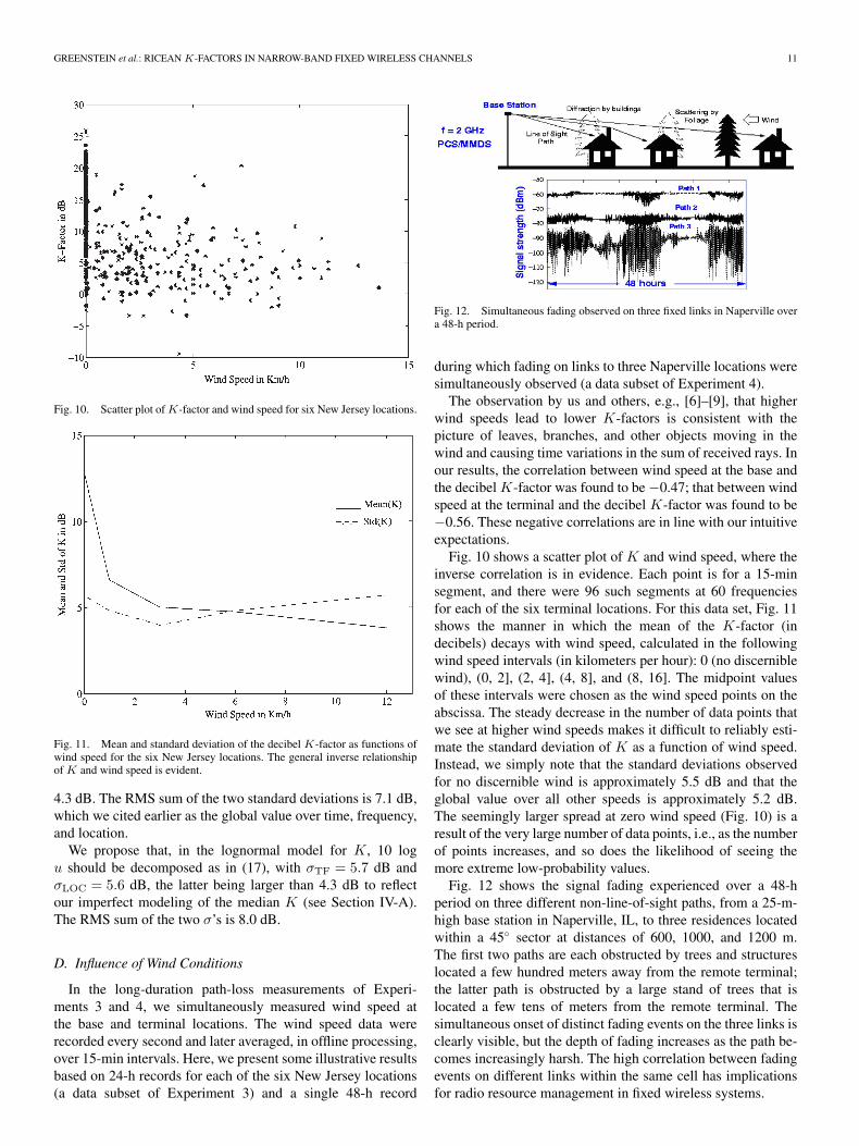
Fig. 10. Scatter plot of K-factor and wind speed for six New Jersey locations.
Fig. 11. Mean and standard deviation of the decibel K-factor as functions ofwind speed for the six New Jersey locations. The general inverse relationshipof K and wind speed is evident.
4.3 dB. The RMS sum of the two standard deviations is 7.1 dB,which we cited earlier as the global value over time, frequency,and location.
We propose that, in the lognormal model for K, 10 logu should be decomposed as in (17), with σTF = 5.7 dB andσLOC = 5.6 dB, the latter being larger than 4.3 dB to reflectour imperfect modeling of the median K (see Section IV-A).The RMS sum of the two σ’s is 8.0 dB.
D. Influence of Wind Conditions
In the long-duration path-loss measurements of Experi-ments 3 and 4, we simultaneously measured wind speed atthe base and terminal locations. The wind speed data wererecorded every second and later averaged, in offline processing,over 15-min intervals. Here, we present some illustrative resultsbased on 24-h records for each of the six New Jersey locations(a data subset of Experiment 3) and a single 48-h record
Fig. 12. Simultaneous fading observed on three fixed links in Naperville overa 48-h period.
during which fading on links to three Naperville locations weresimultaneously observed (a data subset of Experiment 4).
The observation by us and others, e.g., [6]–[9], that higherwind speeds lead to lower K-factors is consistent with thepicture of leaves, branches, and other objects moving in thewind and causing time variations in the sum of received rays. Inour results, the correlation between wind speed at the base andthe decibel K-factor was found to be −0.47; that between windspeed at the terminal and the decibel K-factor was found to be−0.56. These negative correlations are in line with our intuitiveexpectations.
Fig. 10 shows a scatter plot of K and wind speed, where theinverse correlation is in evidence. Each point is for a 15-minsegment, and there were 96 such segments at 60 frequenciesfor each of the six terminal locations. For this data set, Fig. 11shows the manner in which the mean of the K-factor (indecibels) decays with wind speed, calculated in the followingwind speed intervals (in kilometers per hour): 0 (no discerniblewind), (0, 2], (2, 4], (4, 8], and (8, 16]. The midpoint valuesof these intervals were chosen as the wind speed points on theabscissa. The steady decrease in the number of data points thatwe see at higher wind speeds makes it difficult to reliably esti-mate the standard deviation of K as a function of wind speed.Instead, we simply note that the standard deviations observedfor no discernible wind is approximately 5.5 dB and that theglobal value over all other speeds is approximately 5.2 dB.The seemingly larger spread at zero wind speed (Fig. 10) is aresult of the very large number of data points, i.e., as the numberof points increases, and so does the likelihood of seeing themore extreme low-probability values.
Fig. 12 shows the signal fading experienced over a 48-hperiod on three different non-line-of-sight paths, from a 25-m-high base station in Naperville, IL, to three residences locatedwithin a 45◦ sector at distances of 600, 1000, and 1200 m.The first two paths are each obstructed by trees and structureslocated a few hundred meters away from the remote terminal;the latter path is obstructed by a large stand of trees that islocated a few tens of meters from the remote terminal. Thesimultaneous onset of distinct fading events on the three links isclearly visible, but the depth of fading increases as the path be-comes increasingly harsh. The high correlation between fadingevents on different links within the same cell has implicationsfor radio resource management in fixed wireless systems.

12 IEEE TRANSACTIONS ON VEHICULAR TECHNOLOGY
We do not offer the partial results given here as a model forthe dependence of K upon wind speed. We merely use themto illustrate an important physical relationship. For a meaning-ful model development, considerably more experimental datawould be required.
V. CONCLUSION
We have theorized and demonstrated that narrow-band chan-nels in fixed wireless systems can be well modeled by Riceanfading, and we have shown a simple accurate way to computeRicean K-factors from time records of path gain magnitude.The K-factor is a key indicator of the severity of fading; there-fore, modeling its statistics over fixed wireless environments isessential to the study of systems using either narrow-band ormulticarrier radio techniques.
To this end, we have described the collection and reductionof a large body of data at 1.9 GHz for suburban paths in NewJersey, Illinois, and Washington. Whereas other studies havefocused on locations and scenarios in which moving vehiclesand pedestrians have a significant effect on fixed wireless links,we have focused on quiet residential areas where windblowntrees and foliage appear to have the most significant impact. Wehave developed a statistical model that presents K as lognormalover time, frequency, and user location in such environments,with the median being a simple function of season, antennaheight, antenna beamwidth, and distance. Moreover, we haveseparated the variability about the median into two parts: onedue to time and frequency variations per location and one dueto changes among locations. We have also demonstrated theconsistency of key results across different experiments. Finally,we have produced results on the relationship of the K-factorto wind conditions. The results will be useful to those engagedin the design of fixed wireless systems and/or the modeling offixed wireless channels.
ACKNOWLEDGMENT
We are indebted to numerous past and present AT&T col-leagues and contractors for collecting and processing the largequantities of path loss data used in this study. They areD. J. Barnickel, M. K. Dennison, B. J. Guarino, P. B. Guerlain,D. Jacobs, S. C. Kim, R. S. Roman, A. J. Rustako, Jr.,S. K. Wang, J. Lee, L. Roberts and M. Stephano.
REFERENCES
[1] D. Greenwood and L. Hanzo, “Characterization of mobile radio chan-nels,” in Mobile Radio Communications, R. Steele, Ed. London, U.K.:Pentech, 1992, pp. 163–185.
[2] M. Schwartz, W. R. Bennett, and S. Stein, Communication Systems andTechniques. New York: McGraw-Hill, 1966, sec. 9.2.
[3] J. D. Parsons, The Mobile Radio Propagation Channel. Hoboken, NJ:Wiley, 1992, pp. 134–136.
[4] W. C. Jakes, Jr., Ed., Microwave Mobile Communications. New York:Wiley, 1974.
[5] M. J. Gans, N. Amitay, Y. S. Yeh, T. C. Damen, R. A. Valenzuela,C. Cheon, and J. Lee, “Propagation measurements for fixed wireless loops(FWL) in a suburban region with foliage and terrain blockages,” IEEETrans. Wireless Commun., vol. 1, no. 2, pp. 302–310, Apr. 2002.
[6] E. R. Pelet, J. E. Salt, and G. Wells, “Effect of wind on foliage obstructedline-of-sight channel at 2.5 GHz,” IEEE Trans. Broadcast., vol. 50, no. 3,pp. 224–232, Sep. 2004.
[7] D. Crosby, V. S. Abhayawardhana, I. J. Wassell, M. G. Brown, andM. P. Sellars, “Time variability of the foliated fixed wireless access chan-nel at 3.5 GHz,” in Proc. IEEE VTC, May 30–Jun. 1, 2005, pp. 106–110.
[8] M. H. Hashim and S. Stavrou, “Measurements and modeling of windinfluence on radiowave propagation through vegetation,” IEEE Trans.Wireless Commun., vol. 5, no. 5, pp. 1055–1064, May 2006.
[9] H. Suzuki, C. D. Wilson, and K. Ziri-Castro, “Time variation characteris-tics of wireless broadband channel in urban area,” in Proc. 1st Eur. Conf.Antennas Propag., Nice, France, Nov. 2006.
[10] L. Ahumada, R. Feick, and R. A. Valenzuela, “Characterization of tem-poral fading in urban fixed wireless links,” IEEE Commun. Lett., vol. 10,no. 4, pp. 242–244, Apr. 2006.
[11] R. P. Torres, B. Cobo, D. Mavares, F. Medina, S. Loredo, and M. Engels,“Measurement and statistical analysis of the temporal variations of a fixedwireless link at 3.5 GHz,” Wireless Pers. Commun., vol. 37, no. 1/2,pp. 41–59, Apr. 2006.
[12] R. Feick, R. A. Valenzuela, and L. Ahumada, “Experiment results onthe level crossing rate and average fade duration for urban fixed wirelesschannels,” IEEE Trans. Commun., vol. 9, no. 1, pp. 175–179, Jan. 2007.
[13] L. J. Greenstein, S. S. Ghassemzadeh, V. Erceg, andD. G. Michelson, “Ricean K-factors in narrowband fixed wirelesschannels,” in Proc. WPMC, Amsterdam, The Netherlands, 1999.
[14] V. Erceg, “Channel models for fixed wireless applications,” IEEE802.16 Broadband Wireless Access Working Group, IEEE 802.16a-03/01,Jun. 27, 2003.
[15] L. J. Greenstein, D. G. Michelson, and V. Erceg, “Moment-methodestimation of the Ricean K-factor,” IEEE Commun. Lett., vol. 3, no. 6,pp. 175–176, Jun. 1999.
[16] C. Tepedelenlioglu, A. Abdi, and G. B. Giannakis, “The Ricean K factor:Estimation and performance analysis,” IEEE Trans. Wireless Commun.,vol. 2, no. 4, pp. 799–810, Jul. 2003.
[17] Y. Chen and N. C. Beaulieu, “Maximum likelihood estimation of the Kfactor in Ricean fading channels,” IEEE Commun. Lett., vol. 9, no. 12,pp. 1040–1042, Dec. 2005.
[18] V. Erceg, L. J. Greenstein, S. Y. Tjandra, S. R. Parkoff, A. Gupta,B. Kulic, A. A. Julius, and R. Bianchi, “An empirically based path lossmodel for wireless channels in suburban environments,” IEEE J. Sel.Areas Commun., vol. 17, no. 7, pp. 1205–1211, Jul. 1999.
[19] V. Erceg, D. G. Michelson, S. S. Ghassemzadeh, L. J. Greenstein,A. J. Rustako, Jr., P. B. Guerlain, M. K. Dennison, R. S. Roman,D. J. Barnickel, S. C. Wang, and R. R. Miller, “A model for the multipathdelay profile of fixed wireless channels,” IEEE J. Sel. Areas Commun.,vol. 17, no. 3, pp. 399–410, Mar. 1999.
[20] S. R. Hanna and J. C. Chang, “Representativeness of wind measure-ments on a mesoscale grid with station separations of 312 m to 10 km,”Boundary-Layer Meteorol., vol. 60, no. 4, pp. 309–324, Sep. 1992.
[21] M. F. Ibrahim and J. D. Parsons, “Signal strength prediction in built-upareas. Part l: Median signal strength,” Proc. Inst. Elect. Eng.—F, vol. 130,no. 5, pp. 377–384, Aug. 1983.
Larry J. Greenstein (S’59–M’67–SM’80–F’87–LF’02) received the B.S., M.S., and Ph.D. degreesin electrical engineering from the Illinois Instituteof Technology, Chicago, in 1958, 1961, and 1967,respectively.
From 1958 to 1970, he was with IIT ResearchInstitute, Chicago, working on radio frequency inter-ference and anticlutter airborne radar. He joinedBell Laboratories, Holmdel, NJ, in 1970. He waswith AT&T for 32 years, conducting research ondigital satellites, point-to-point digital radio, optical
transmission techniques, and wireless communications. For 21 years duringthat period (1979–2000), he led a research department renowned for itscontributions in these fields. He is currently a Research Scientist with theWireless Information Network Laboratory (WINLAB), Rutgers University,North Brunswick, NJ, working in the areas of ultrawideband, sensor net-works, multiple-input–multiple-output-based systems, broadband power linesystems, and radio channel modeling. He has been a Guest Editor, SeniorEditor, and Editorial Board Member for numerous publications.
Dr. Greenstein is an AT&T Fellow. He is a recipient of the IEEE Com-munications Society’s Edwin Howard Armstrong Award and a corecipient offour best paper awards. He is currently the Director of Journals for the IEEECommunications Society.

GREENSTEIN et al.: RICEAN K-FACTORS IN NARROW-BAND FIXED WIRELESS CHANNELS 13
Saeed S. Ghassemzadeh (S’88–M’91–SM’02) re-ceived the B.S., M.S., and Ph.D. degrees in electricalengineering from the City University of New York,New York, in 1989, 1991, and 1994, respectively.
From 1989 to 1992, he was with SCS Mobile-com, which is a wireless technology developmentcompany, where he conducted research in the areasof wireless channel modeling. In 1992, while work-ing toward the Ph.D. degree, he joined InterDigital,where he worked as a Principal Research Engineer,conducting research in the areas of fixed/mobile
wireless channels, and was involved in system integration and testing ofB-code-division multiple access (CDMA) technology. At the same time, hewas also an Adjunct Lecturer with the City University of New York. In1995, he joined AT&T Wireless Communication Center of Excellence, AT&TBell Laboratories, where he was involved in the design and developmentof the fixed wireless base station. He also conducted research in areas ofCDMA technologies, propagation channel measurement and modeling, satellitecommunications, wireless local area networks, and coding in wireless systems.He is currently Principal Member of Technical Staff with the CommunicationTechnology Research Department at AT&T Labs-Research, Florham Park,NJ. His current research interest includes wireless propagation measurementand modeling, cognitive radio, wireless local area networks, and terahertzcommunications.
Dr. Ghassemzadeh is a member of the IEEE Communication Society andIEEE Vehicular Technology Society. He is currently an Associate Editor for theIEEE TRANSACTIONS ON WIRELESS COMMUNICATIONS and the Journal ofCommunications and Networks.
Vinko Erceg (M’92–SM’98–F’07) received theB.Sc. degree in electrical engineering and the Ph.D.degree in electrical engineering from the City Uni-versity of New York, in 1988 and 1992, respectively.
From 1990 to 1992, he was a Lecturer with theDepartment of Electrical Engineering, City Collegeof the City University of New York. Concurrently,he was a Research Scientist with SCS Mobilecom,Port Washington, NY, working on spread-spectrumsystems for mobile communications. In 1992, hejoined AT&T Bell Laboratories. In 1996, he joined
AT&T Labs—Research as a Principal Member of Technical Staff with theWireless Communications Research Department, where he worked on signalpropagation and other projects related to the systems engineering and perfor-mance analysis of personal and mobile communication systems. From 2000 to2002, he was with Iospan Wireless Inc., San Jose, CA, as the Director of theCommunication Systems Division, working on system, propagation, deploy-ment, and performance issues of a multiple-input–multiple-output orthogonalfrequency division multiplexing communication system. He is currently aSenior Manager with the Broadcom Corporation, San Diego, CA.
David G. Michelson (S’80–M’89–SM’99) receivedthe B.A.Sc., M.A.Sc., and Ph.D. degrees in electricalengineering from the University of British Columbia(UBC), Vancouver, BC, Canada.
From 1996 to 2001, he served as a member of ajoint team from AT&T Wireless Services, Redmond,WA, and AT&T Labs—Research, Red Bank, NJ,where he was concerned with the development ofpropagation and channel models for next-generationand fixed wireless systems. The results of this workformed the basis for the propagation and channel
models later adopted by the IEEE 802.16 Working Group on Broadband FixedWireless Access Standards. From 2001 to 2002, he helped to oversee thedeployment of one of the world’s largest campus wireless local area networksat UBC while also serving as an Adjunct Professor with the Department ofElectrical and Computer Engineering. Since 2003, he has led the Radio ScienceLaboratory, Department of Electrical and Computer Engineering, UBC, wherehis current research interests include propagation and channel modeling forfixed wireless, ultra wideband, and satellite communications.
Prof. Michelson is a registered professional engineer. He serves as the Chairof the IEEE Vehicular Technology Society Technical Committee on Propaga-tion and Channel Modeling and as an Associate Editor for Mobile Channelsfor IEEE Vehicular Technology Magazine. In 2002, he served as a Guest Editorfor a pair of Special Issues of the IEEE JOURNAL ON SELECTED AREAS IN
COMMUNICATIONS concerning propagation and channel modeling. From 2001to 2007, he served as an Associate Editor for the IEEE TRANSACTIONS ON
VEHICULAR TECHNOLOGY. From 1999 to 2007, he was the Chair of the IEEEVancouver Section’s Joint Communications Chapter. Under his leadership, thechapter received Outstanding Achievement Awards from the IEEE Communi-cations Society in 2002 and 2005 and the Chapter of the Year Award from IEEEVehicular Technology Society in 2006. He received the E. F. Glass Award fromIEEE Canada in 2009.

IEEE TRANSACTIONS ON VEHICULAR TECHNOLOGY 1
Ricean K-Factors in Narrow-Band Fixed WirelessChannels: Theory, Experiments, and
Statistical ModelsLarry J. Greenstein, Life Fellow, IEEE, Saeed S. Ghassemzadeh, Senior Member, IEEE,
Vinko Erceg, Fellow, IEEE, and David G. Michelson, Senior Member, IEEE
Abstract—Fixed wireless channels in suburban macrocells aresubject to fading due to scattering by moving objects such aswindblown trees and foliage in the environment. When, as is oftenthe case, the fading follows a Ricean distribution, the first-orderstatistics of fading are completely described by the correspondingaverage path gain and Ricean K-factor. Because such fading hasimportant implications for the design of both narrow-band andwideband multipoint communication systems that are deployed insuch environments, it must be well characterized. We conducted aset of 1.9-GHz experiments in suburban macrocell environmentsto generate a collective database from which we could construct asimple model for the probability distribution of K as experiencedby fixed wireless users. Specifically, we find K to be lognormal,with the median being a simple function of season, antenna height,antenna beamwidth, and distance and with a standard deviationof 8 dB. We also present plausible physical arguments to explainthese observations, elaborate on the variability of K with time,frequency, and location, and show the strong influence of windconditions on K .
Index Terms—Fading, fixed wireless channels, K-factors, multi-point communication, Ricean distribution.
I. INTRODUCTION
DURING the past decade, both common carriers and utili-ties have begun to deploy fixed wireless multipoint com-
munication systems in suburban environments. For commoncarriers, wideband multipoint communication systems providea method for delivering broadband voice and data to residenceswith greater flexibility than wired services. For utilities, narrow-band multipoint communication systems provide a convenientand independent method for controlling or monitoring theinfrastructure, including utility meters located on customerpremises. In the past, most narrow-band fixed wireless links
Manuscript received June 26, 2008; revised December 18, 2008. The reviewof this paper was coordinated by Dr. K. T. Wong.
L. J. Greenstein is with the Wireless Information Network Laboratory,Rutgers University, North Brunswick, NJ 08902 USA (e-mail: [email protected]).
S. S. Ghassemzadeh is with the Communication Technology ResearchDepartment, AT&T Labs-Research, Florham Park, NJ 07932 USA (e-mail:[email protected]).
V. Erceg is with the Broadcom Corporation, San Diego, CA 92128 USA(e-mail: [email protected]).
D. G. Michelson is with the Radio Science Laboratory, Department of Elec-trical and Computer Engineering, University of British Columbia, Vancouver,BC V6T 1Z4, Canada (e-mail: [email protected]).
Color versions of one or more of the figures in this paper are available onlineat http://ieeexplore.ieee.org.
Digital Object Identifier 10.1109/TVT.2009.2018549
were deployed in frequency bands below 900 MHz. In responseto increasing demand, both the Federal Communication Com-mission and Industry Canada have recently allocated severalnew bands between 1.4 and 2.3 GHz to such applications. Be-cause fading on fixed wireless links has important implicationsfor the design of both narrow-band and wideband multipointcommunication systems, it must be well characterized. Narrow-band fading models apply to both narrow-band signals and in-dividual carriers or pilot tones in orthogonal frequency-divisionmultiplexing systems such as those based upon the IEEE 802.16standard. Ideally, such models will capture not just the statisticsof fading but their dependence upon the type and density ofscatterers in the environment as well.
The complex path gain of any radio channel can quitegenerally be represented as having a fixed component plus afluctuating (or scatter) component. The former might be dueto a line-of-sight path between the transmitter and the receiver;the latter is usually due to echoes from multiple local scatterers,which causes variations in space and frequency of the summedmultipath rays. The spatial variation is translated into a timevariation when either end of the link is in motion. In the case offixed wireless channels, time variation is a result of scatterersin motion.
If the scatter component has a complex Gaussian distribution,as it does in the central limit (many echoes of comparablestrength), the time-varying magnitude of the complex gain willhave a Ricean distribution. The key parameter of this distribu-tion is the Ricean K-Factor (or just K), which is the power ratioof the fixed and scatter components [1]–[3]. It is a measure ofthe severity of fading. The case K = 0 (no fixed component)corresponds to the most severe fading, and in this limiting case,the gain magnitude is said to be Rayleigh distributed. From theearliest days, most analyses of mobile cellular systems, e.g., [4],have assumed Rayleigh fading because it is both conservativeand quite prevalent.
The case of fixed wireless paths, e.g., for wireless multipointcommunication systems, is different. Here, there can still bemultipath echoes, and the complex sums of received wavesstill vary over space and frequency. However, with both endsof the link fixed, there will be—to first order—no temporalvariations. What alters this first-order picture is the slow motionof scatterers along the path, e.g., pedestrians, vehicles, andwind-blown leaves and foliage. As a result, the path gain atany given frequency will exhibit slow temporal variations as
0018-9545/$25.00 © 2009 IEEE

2 IEEE TRANSACTIONS ON VEHICULAR TECHNOLOGY
the relative phases of arriving echoes change. Because theseperturbations are often slight, the condition of a dominant fixedcomponent plus a smaller fluctuating component takes on ahigher probability than that for mobile links. Furthermore, sincetemporal perturbations can occur on many scatter paths, theconvergence of their sum to a complex Gaussian process isplausible. Therefore, we can expect a Ricean distribution forthe gain magnitude, with a higher K-factor, in general, thanthat for mobile cellular channels.
During the past decade, numerous studies have aimed toreveal various aspects of the manner in which fixed wirelesschannels fade on non-line-of-sight paths typical of those en-countered in urban and suburban environments [5]–[12]. Oneset of researchers has focused on determining the manner inwhich wind blowing through foliage affects the depth of fadingon fixed links, e.g., [6]–[9], while another has focused on sce-narios in which relatively little foliage is present but scatteringfrom vehicular traffic presents a significant impairment, e.g.,[10]–[12].
In this paper, we focus on the development of statisticalmodels that capture the manner in which fading on fixedwireless channels in suburban macrocell environments dependsupon the local environment, the season (leaves or no leaves),the distance between the base and the remote terminal, andthe height and beamwidth of the terminal antenna. We do sousing an extensive body of data collected during four distinctexperiments. Our earlier findings were presented in [13] andwere ultimately adopted by IEEE 802.16 [14]. Here, we fill inthe essential detail concerning the measurement campaigns andpresent plausible physical arguments to explain our observa-tions. Furthermore, we demonstrate that the variability of thechannel about the median can be divided into a componentdue to variation at a fixed location and another due to variationbetween locations. Finally, we present what we believe are thefirst observations of simultaneous fading events on differentlinks within the same suburban macrocell.
In Section II, we review a method for computing K fromtime records of path gain magnitude that is particularly fastand robust and therefore suited to high-volume data reductions.We show that it is also highly accurate. In Section III, wedescribe several experiments that were conducted at 1.9 GHz tomeasure path gains on fixed wireless links. The data from theseexperiments were used to compute K-factors for narrow-bandchannels. In Section IV, we show how the computed resultswere used to model the statistics of K as a function of variousparameters. We also examine such issues as the variability ofK with time, frequency, and location and the influence of windconditions on K. Section V concludes the paper.
II. ESTIMATION OF RICEAN K-FACTOR
A. Background
Our practical objective is to model narrow-band fading bymeans of a Ricean distribution over the duration of a fixed wire-less connection. We assume that the duration of a connection isin the 5–15-min range, and we will compute K for finite timeintervals of that order. Later, we will show how K can varywith the time segment and with frequency. We will also show
that the statistical model for K is very similar for 5- and 15-minintervals.
B. Formulation
We characterize the complex path gain of the narrow-bandwireless channel by a frequency-flat time-varying response
g(t) = V + v(t) (1)
where V is a fixed complex value, and v(t) is a complex zero-mean random time fluctuation caused by vehicular motion,wind-blown foliage, etc., with variance σ2. This descriptionapplies to a particular frequency and time segment. Both V andσ2 may change from one time–frequency segment to another.
We assume that the quantity actually measured is the receivednarrow-band power, which, suitably normalized, yields theinstantaneous power gain
G(t) = |g(t)|2 . (2)
Various methods have been reported to estimate K usingmoments calculated from time series such as (2), e.g.,[15]–[17].
We can relate K to two moments that can be estimated fromthe data record for G(t). The first moment Gm is the averagepower gain; its true value (as distinct from the estimate
Gm =N∑
i=1
Gi
n(3)
computed from finite data) is shown in [15] to be
Gm = |V |2 + σ2. (4)
The second moment Gv is the RMS fluctuation of G aboutGm. The true value of this moment (as distinct from theestimate
Gv =
√√√√ 1N
N∑i=1
(Gi − Gm)2 (5)
calculated from finite data) is shown in [15] to be
Gm =√
σ4 + 2|V |2σ2. (6)
In each of (4) and (6), the left-hand side can be estimatedfrom the data, and the right-hand side is a function of the twointermediate quantities we seek. Combining these equations,we can solve for |V |2 and σ2, yielding
|V |2 =√
G2m − G2
v (7)
σ2 = Gm −√
G2m − G2
v. (8)
Finally, K is obtained by substituting these two values into
K = |V |2/σ2. (9)
Note that σ2 as defined here is twice the RF power of thefluctuating term, which is why the customary factor of two
GREENSTEIN et al.: RICEAN K-FACTORS IN NARROW-BAND FIXED WIRELESS CHANNELS 3
Fig. 1. Four typical envelope cdf’s, comparing actual data (solid curves) withRicean distributions (dashed curves). The latter use K-factors derived from datavia the moment method.
(see [3, eq. (5.60)]) is not present in (9). The K-factor andaverage power gain Gm jointly determine the Ricean envelopedistribution.
The choice of the measurement interval is a necessary com-promise between obtaining a large sample size and preservingthe stationarity within the interval. Given the rate at whichmeteorological conditions, particularly wind conditions, usu-ally change, we considered 15 min to be suitably small. Thissupposition is supported by the consistency of our results for 5-and 15-min segments.
C. Validation
For each of several fixed wireless paths located in suburbanNew Jersey, we collected 5-min time sequences of receivedpower at 1.9 GHz (see Section III). For each path, we can com-pute a cumulative distribution function (cdf) of the measuredsamples. This is the empirical cdf of the received envelope. Wecan also estimate Gm and K, the two parameters that define aRicean distribution, and then compute a Ricean distribution thatshould closely match the empirical one.
Comparisons for four typical cases are shown in Fig. 1.Each corresponds to a particular time, frequency, andtransmit–receive path. In each case, the results show that, al-though some cases fit better than others, the Ricean distributionobtained using the estimated moments is quite close to the em-pirical one. Deviation from the ideal can usually be interpretedas the result of a transient fading event affecting the distributionof either the fixed or scatter component. In the absence of moredetailed information, e.g., time- and/or angle-of-arrival data, itis difficult to offer further interpretation of a given result.
We also examined goodness-of-fit methods to determineK. Although they are accurate, they are also much more timeintensive and, thus, not conducive to the reduction of largequantities of data [1]. Moreover, they produce results not
Fig. 2. Comparisons, for each of two locations, of K versus f , where K isderived via two methods: the moment method and the least-mean-square fittingof empirical and Ricean distributions. These results are typical and show thatthe moment method predicts K to within 2 dB (usually much less) of the resultsfor least-mean-square fitting.
much different from those using the moment method. Fig. 2gives two typical comparisons, based upon data collected insuburban New Jersey, in each of which K-factors at differentfrequencies over a 9-MHz bandwidth are shown for both themoment method and the goodness-of-fit method. The latterconsisted of matching the data-derived cdf of G to a Riceanone, with K chosen to minimize the RMS decibel differencebetween cdf’s over the probability range from 1% to 50%.
We note that, if the calculated moment Gv exceeds the calcu-lated moment Gm, the calculated result for |V |2, from (7), willbe imaginary. When this happens, it is because either 1) the un-derlying process is not well modeled as Ricean, or 2) the statis-tical noise of the finite time record produces a Gv slightly largerthan Gm instead of being equal to or slightly smaller than Gm.
In our reductions, we declare K to be 0.1 if Gv exceedsGm by less than 0.5 dB1; if it is larger than that, we removethe particular record from the database. In our reductions of5-min records, such removals occurred in a small fraction ofall cases (less than 2%). In our reductions of 15-min records,the fraction was even smaller.
Typical 5-min records of received decibel power are shown inFig. 3. Such records, converted to linear power and suitably nor-malized, yield records of G(t), as given in (2). Our examinationof data like these indicate that relatively shallow fluctuations, ona time scale of 1 or 2 s, occur on most links, in addition to possi-bly deeper fluctuations on a time scale of tens of seconds [18].
D. Properties of the Ricean K-Factor
The complex fluctuation v(t), from (1), for a given frequencyis due to temporal variations in gain on one or more paths.If these variations are independent among paths, then the
1Over the range below 0.1, the precise value of K is immaterial. For allpractical system purposes, it is zero, but we assign it a value 0.1 (−10 dB) forconvenience in tabulating statistics.
4 IEEE TRANSACTIONS ON VEHICULAR TECHNOLOGY
Fig. 3. Two typical examples of measured path gain at a particular frequencyover 280 s. Note that fading can be quite deep and that temporal fluctuationrates are on a scale of hertz or lower.
Fig. 4. Two typical examples of the fixed and mean-square “scatter” com-ponents of path gain, as functions of frequency. Note that σ2 is fairly flatwith frequency, so that the frequency variation of K = |V |2/σ2 follows thatof |V |2.
mean-square value of v(t) will be flat with frequency. [To seethis, write v(t) as the response at a given frequency to a sumof delayed echoes, where the echoes have time-varying inde-pendent gains of zero mean. Next, derive the ensemble mean of|v(t)|2, and note that it is independent of the given frequency.]This result is observed in the sample plots, in Fig. 4, of |V |2 andσ2 versus frequency. These plots are typical of what we observeon most links, i.e., σ2 exhibits a relative flatness with frequency,with the small perturbations being attributable to statisticaleffects. Since K is the ratio of |V |2 to σ2, we conclude thatits variation with frequency is essentially proportional to that ofthe fixed gain component. This, in turn, depends on the complexamplitude versus delay of the significant echoes, which variesfrom one transmit–receive path to another [19].
Other properties of the Ricean K-factor can be anticipatedby similar reasoning.
1) At a given distance, we might suppose that the strength ofthe scatter component, which is the result of rays comingfrom a multiplicity of directions, will vary far less thanthe strength of the fixed component, which is dominatedby rays coming from the direction of the base station andwhich will be strongly affected by local shadowing alongthat direction. Thus, we expect K to exhibit lognormalstatistics across locations, with a standard deviation com-parable to that associated with shadow fading.
2) By definition, remote terminals in macrocell environ-ments generally lie in the shadow region of the obstaclesthat block its line of sight to the base station. As the heightof the terminal antenna increases, the diffraction anglewill decrease, and the strength of the fixed componentwill increase. Again, we might suppose that the scattercomponent, which is the result of reflection and scatteringfrom a multiplicity of directions, will vary far less withthe terminal height than the fixed component. Thus, weexpect K to increase with the terminal height.
3) Because the scattered component will come from allother directions, increasingly less of the scatter signal willbe received as the beamwidth of the receiving antennadecreases. Thus, we expect K to increase as the antennabeamwidth decreases.
4) Previous work has shown that the average wind velocityabove treetop level does not vary much over distancesof several kilometers [20]. Thus, we expect that fadingevents associated with windblown foliage should be fairlywell correlated between links within a typical cell.
In the next section, we describe the experiments that we con-ducted to investigate the validity of these and other conjectures.
III. MEASUREMENT PROGRAM
The database used in our modeling comes from four distinctexperiments conducted in suburban areas, as summarized inTable I. Each of the four experiments has its own purposes,strengths, and limitations but had, as one of its objectives, thedetermination of K-factors on fixed wireless paths. Collec-tively, this set has provided an extensive body of data fromwhich Ricean K-factors can be computed and modeled. Wedescribe the four experiments in this section and report theK-factors reduced from them in the next section. It should benoted that fading on the uplink and downlink are reciprocal forthe same path and frequency and that all the measurementsreported here were for the downlink only. Furthermore, allmeasurements were made using an equipment van parked onthe street, with the terminal antenna pointed to receive themaximum downlink signal. All of our data were collected inquiet residential neighborhoods with minimum residential andpedestrian traffic.
We characterized each neighborhood according to the gen-eral nature of both the terrain and the trees and foliage but didnot attempt to characterize vegetation density or building-to-lotarea ratios along individual paths. Whereas such an approachwas used in [21] to assist in the prediction of mean path loss inurban environments, our measurement database, large as it is,is insufficient to take full advantage of such detail.

GREENSTEIN et al.: RICEAN K-FACTORS IN NARROW-BAND FIXED WIRELESS CHANNELS 5
TABLE ISUMMARY OF THE FOUR EXPERIMENTS
A. Experiment 1: Short-Term Measurements in New Jersey
Downlink measurements were made for three transmit sitesin northern and central New Jersey. For each site, data were col-lected at 33 or more downlink locations during summer (treesin full bloom), and repeat measurements were made at half ormore of these locations during winter (trees bare). Distancesranged (more or less uniformly) from 0.5 to 9 km. This was themajor experiment in our study, and so, we summarize a numberof its features in Table II.
The transmit sites were located in the residential communi-ties of Holmdel, Whippany, and Clark. Each site overlookeda terrain consisting of rolling hills with moderate to heavy treedensities and dwellings of one or two stories. Furthermore, eachsite used a panel-type transmitting antenna with elevation andazimuth beamwidths of 16◦ and 65◦, respectively. The antennawas fed by a 10-MHz swept frequency generator centered at1985 MHz.
For each downlink location (i.e., receive terminal site) foreach of two antennas at each of two heights (3 and 10 m),the data record consists of 700 “snapshots” of received powerversus frequency. The receiver was a swept frequency spectrumanalyzer equipped with a low noise amplifier to increase itssensitivity; its sweep was synchronized to that of the transmit-ter using the 1-pulse-per-second signal from a GPS receiver.The unit was operated in sample detection mode to enhanceits ability to characterize the first-order statistics of randomsignals. A local controller handled the configuration, operation,and data acquisition. The “snapshots” for each antenna/heightcombination are spaced by 0.4 s, for a total time span of nearly5 min, and each consists of 90 samples, spaced by 100 kHz,for a frequency span of 9 MHz. In the data processing, thepower samples, which were recorded in decibels of the mea-sured power referenced to 1 mW (dBm), were calibrated andconverted to linear path gain.
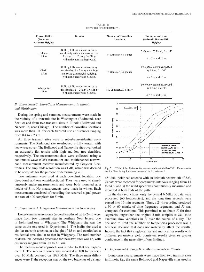
6 IEEE TRANSACTIONS ON VEHICULAR TECHNOLOGY
TABLE IIFEATURES OF EXPERIMENT 1
B. Experiment 2: Short-Term Measurements in Illinoisand Washington
During the spring and summer, measurements were made inthe vicinity of a transmit site in Washington (Redmond, nearSeattle) and from two transmit sites in Illinois (Bellwood andNaperville, near Chicago). The number of downlink locationswas more than 100 for each transmit site at distances rangingfrom 0.4 to 2.2 km.
All three transmit sites were in suburban/residential envi-ronments. The Redmond site overlooked a hilly terrain withheavy tree cover. The Bellwood and Naperville sites overlookedan extremely flat terrain with high and low tree densities,respectively. The measurement data were collected using acontinuous-wave (CW) transmitter and multichannel narrow-band measurement receiver manufactured by Grayson Elec-tronics. The amplitude resolution was 1 dB, which was deemedto be adequate for the purpose of determining K.
Two antennas were used at each downlink location: onedirectional and one omnidirectional. They were used to simul-taneously make measurements and were both mounted at aheight of 3 m. No measurements were made in winter. Eachmeasurement consisted of recording the received signal powerat a rate of 400 samples/s for 5 min.
C. Experiment 3: Long-Term Measurements in New Jersey
Long-term measurements (record lengths of up to 24 h) weremade from two transmit sites in northern New Jersey: onein Iselin and one in Whippany. The Whippany site was thesame as the one used in Experiment 1. The Iselin site used asimilar transmit antenna, at a height of 15 m, and overlooked aresidential area similar to that in Whippany. The total numberof downlink locations processed for these two sites was 16, withdistances ranging from 0.5 to 3.1 km.
The measurement approach was similar to that for Experi-ment 1: The received power was recorded at 100 frequenciesover 10 MHz centered on 1985 MHz. The three main differ-ences were 1) the reception was on the two branches of a slant-
Fig. 5. CDFs of the K-factor for an antenna beamwidth of 30◦. These resultsare for New Jersey locations measured in Experiment 1.
45◦ dual-polarized antenna with an azimuth beamwidth of 32◦,2) data were recorded for continuous intervals ranging from 11to 24 h, and 3) the wind speed was continuously measured andrecorded at both ends of the path.
In the data reductions, only the central 6 MHz of data wereprocessed (60 frequencies), and the long time records wereparsed into 15-min segments. Thus, a 24-h recording produceda 96 × 60 matrix of time–frequency segments, and K wascomputed for each one. This permitted us to obtain K for timesegments longer than the original 5-min samples as well as toexamine slow variations in K over the course of a day. Thedecision to limit the number of frequencies processed was abusiness decision that does not materially affect the results.Indeed, the fact that single-carrier and multicarrier results withdifferent parameters yield consistent results gives us greaterconfidence in the generality of our findings.
D. Experiment 4: Long-Term Measurements in Illinois
Long-term measurements were made from two transmit sitesin Illinois, i.e., the same Bellwood and Naperville sites used in

GREENSTEIN et al.: RICEAN K-FACTORS IN NARROW-BAND FIXED WIRELESS CHANNELS 7
TABLE IIIMEDIAN K-FACTORS FOR EXPERIMENT 1∗
Experiment 2. For Bellwood, there were 14 downlink locations,at distances ranging from 0.35 to 1.4 km; for Naperville, therewere 21 downlink sites, at distances ranging from 0.6 to 2.1 km.
The measurement approach was similar to that of Experi-ment 2, with differences similar to those between Experi-ments 1 and 3: 1) the use of dual-polarized slant-45◦ antennaswith 32◦ beamwidths; 2) the long-term data records, withmeasurements ranging from 2 to 12 h; and 3) the measurementand recording of wind speed.
IV. RESULTS
A. First-Order Statistical Model for K
General: By a “first-order statistical model,” we mean onethat gives the probability distribution of K, given a set ofpath and system parameters, e.g., distance, season, terminalantenna height, and terminal antenna beamwidth, based uponmeasurements collected over time, frequency (in the case ofmulticarrier signals), and location. A “second-order statisticalmodel” would, in addition, sort out the individual variationswith time, frequency, and location. We provide some results onthat aspect in Section IV-C.
The model we present here is entirely based on the databasefor Experiment 1, which is the richest in terms of parametervariation. However, we will expand this model and confirm itsvalidity by using results from the other three experiments.
Database: Each short-term measurement in New Jersey ini-tially produced 750 “snapshots,” spaced by 0.4 s, of receivedpower versus frequency at 100 frequencies spaced by 100 kHz.For convenience in the data reductions, however, each recordwas trimmed to 700 “snapshots” (280-s time span) and90 frequencies (9-MHz frequency span). We thus computed90 K-factors, each using recorded power versus time over4.67 min. In only 1% of all cases did the method in Section IIfail to produce a real solution for K.
K-Factor Medians: As noted in Table I, the database en-compasses two seasons [summer (leaves) and winter (noleaves)], two antenna heights (3 and 10 m), and three antennabeamwidths (17◦, 30◦, and 65◦), for a total of 12 combinations.For each parameter set (season, height, and beamwidth), wecomputed K over a large population of frequencies and loca-tions and then computed a cdf. One such result is shown inFig. 5, which shows four cases (2 seasons × 2 heights) for agiven beamwidth. To compress the information in curves like
Fig. 6. CDF of the K-factor variation about the distance regression line forthe data of Experiment 1. The closeness to a straight line on this scale impliesa near-lognormal distribution. The slope implies a standard deviation of 8 dB.
this, we extracted the median K for all the cdf’s and analyzedthe 12 values. These values are summarized in Table III,rounded to the nearest 0.5 dB.
Methodology: First, we examine the influence of season(leaves versus no leaves). For the six combinations of twoantenna heights and three antenna beamwidths, we see a con-sistent increase in median K from summer to winter, rangingfrom 3.5 to 4.5 dB with an average close to 4.0 dB (or 2.5 inlinear units). We attribute the increase to the reduction in gainvariations when there are no windblown leaves.
Second, we examine the influence of antenna height h. Forthe two seasons and three beamwidths, we see a consistentincrease from 3 to 10 m, ranging from 2.0 to 3.0 dB withan average of 2.4 dB. If we assume a power-law relationship,i.e., K ∝ hα, then α = 0.46. This modest increase with his consistent with intuition: we expect there to be a gradualincrease in line-of-sight power (which is generally fixed intime) as the terminal antenna height increases. In hindsight,it would have been preferable to collect data at three heightsrather than just two. On the other hand, such trends, particularlyover a limited range of values as in this case, are almost alwaysapproximately linear on a log–log plot, indicating a power-law relationship. It is unlikely that the true decibel values for

8 IEEE TRANSACTIONS ON VEHICULAR TECHNOLOGY
TABLE IVSUMMARY OF RESULTS FOR EXPERIMENT 2
heights in between would seriously be different from what thepower-law relationship predicts. Because the behavior of Kwith height will change as the terminal antenna rises out of thelocal clutter, care should be taken not to extrapolate beyond theheight of the clutter.
Third, we examine the influence of antenna beamwidth b. Inthe Holmdel measurements, beamwidths of 17◦ and 65◦ wereused in simultaneous measurements. The difference in medianK between these two beamwidths ranges from 3.0 to 4.0 dB,with an average of about 3.6 dB. If we assume a power-lawrelationship, i.e., K ∝ bβ , then β = −0.62. When we apply thislaw to the medians for b = 30◦, which were collected elsewhere(Clark and Whippany), the agreement is within 1 dB.
The result for β is particularly satisfying. If there wasno angular scatter, we would expect to see β = 0 (K-factorunaffected by beamwidth), and if the scatter were uniformin strength over 360◦ in azimuth, we would expect to seeβ = −1.0 (K-factor directly proportional to antenna gain).The value β = −0.62 is consistent with an environment ofsignificant but not totally uniform scatter.
Finally, we consider the influence of distance d. If we assumea power-law relationship, i.e., K ∝ dγ , then the aforementionedresults lead us to the formulation
K ∼= FsFhFbKodγ (d in kilometers) (10)
where the factors are defined as follows.1) Fs is the seasonal factor
Fs ={
1.0, Summer (Leaves)2.5; Winter (No Leaves).
(11)
2) Fh is the height factor
Fh = (h/3)0.46 (h in meters). (12)
3) Fb is the beamwidth factor
Fb = (b/17)−0.62 (b in degrees). (13)
Ko and γ are constants to be optimized via regression fitting.Now, we form the data variable
Y = K/(FsFhFb) ∼= Kodγ . (14)
Fig. 7. CDFs of the K-factors computed for Naperville, IL, in Experi-ment 2. Both results show near-lognormal distributions. The standard deviationis similar for each (slightly above 6 dB), but the median for the directionalantenna is roughly 6 dB higher than that for the omnidirectional antenna.
For every K computed in the database, there is an associatedseason, height, beamwidth, and distance, and so, a Y valuecan be computed and paired with d. We can then perform aregression fit between Y and d over the database.2
The result we get is that Ko∼= 10.0 dB and γ ∼= −0.5 dB.
The standard deviation of 10 log Y about the regression curveis just under 8.0 dB. Moreover, the distribution of 10 log Yabout that curve is very nearly Gaussian, as seen in Fig. 6.The meaning is that K can be very accurately modeled as alognormal variable, with a median value easily related to pathand system parameters.
Summary of the First-Order Model: At any time, frequency,and location, the K-factor in a given season, for a given antenna
2We are implicitly assuming a common distance dependence for all parame-ter combination, which is an assumption not fully vindicated by the data. Wewill see that the price for this simplification is a modest increase in variabilityabout the median.

GREENSTEIN et al.: RICEAN K-FACTORS IN NARROW-BAND FIXED WIRELESS CHANNELS 9
TABLE VSUMMARY OF RESULTS FOR EXPERIMENT 4
height, antenna beamwidth, and distance, can be described asfollows in a suburban New Jersey type of terrain:
K = K1dγu (15)
where K1 is the 1-km intercept
K1 = Fs · Fh · Fb · Ko (16)
Ko∼= 10.0 dB; γ ∼= −0.5; Fs, Fh, and Fb are given by
(9)–(11); and u is a lognormal variate, whose decibel value iszero mean with a standard deviation σ of 8.0 dB.
We observe that, for each of the 12 parameter sets identifiedearlier, the standard deviation about the decibel median for thatset was about 7 dB, or a bit more. The increase of less than1 dB in σ is mostly due to simplifications in modeling themedian, including assuming a common distance dependencefor all parameter sets. This small degree of added variabilityis a minor price for obtaining a simple and user-friendly model.
B. Consistency Checks
The reduced results from Experiment 2 are summarizedin Table IV. In computing K via (1)–(9), the percentage ofdata removed because K was not real was 0%, 1%, and 2%for Redmond, Naperville, and Bellwood, respectively, with nodifference between omnidirectional and directional antennas.We make the following observations.
1) The main difference between the terrains in Bellwoodand Naperville is tree density (high in Bellwood andlow in Naperville). The roughly 4-dB higher values forK1 in Naperville (3.7 and 4.3 dB for omnidirectionaland directional antennas, respectively) match the seasonaldifference for New Jersey (leaves versus no leaves).
2) The higher values of K1 for the directional antennasclosely follow the beamwidth dependence given by (13),which predicts a 5.6-dB increase for the 45◦ beamwidthused in Illinois and a 6.7-dB increase for the 30◦
beamwidth used in Washington. The agreements (within1 dB) are exceptionally good, particularly since (13) wasempirically derived for beamwidths of 65◦ and below.
3) The values of K1 for Bellwood and Naperville (takingproper account of the beamwidth and season) are within0.5 dB of the values predicted by the first-order model.
4) The numerical values for γ and σ in Table IV are con-sistent with those for the first-order model. The distanceexponent is smaller in some cases, and so is the standarddeviation. However, the data volume for Experiment 2 isnot large enough for these differences to be statisticallysignificant. What the tabulations show that is significantis that σ does not change with antenna beamwidth, inagreement with the first-order model.
5) The cdf’s of K in Illinois and Washington show the samelognormal character predicted by the first-order model.For example, Fig. 7 shows cdf’s of K, for both antennatypes, in Bellwood.
Now, moving to Experiment 3, we present a result that showsa remarkable consistency with the first-order model: Over60 frequencies and up to 96 time segments at 16 locations,K was found to be essentially lognormal, with a median andstandard deviation of 8.5 and 7.1 dB, respectively. Since thesedata were for distances uniformly clustered between 0.5 and2.0 km, the median closely corresponds to the 1-km interceptof the model, i.e., K1 in (16). For the conditions summer,h = 3 m, and b = 32◦, the model predicts K1 to be 8.3 dB.Furthermore, the 7.1-dB standard deviation is close to the8.0-dB model value, which is slightly elevated due to modelingapproximations.
Note that Experiments 1 and 3 were conducted on differ-ent paths, in different years, using two different measurementintervals (5 and 15 min) and different antenna types. Givenall that, the agreement in the global statistics of K is indeedremarkable.
Somewhat less affirming is a comparison with the resultsfrom Experiment 4, summarized in Table V. On the positiveside, these results repeat the increase in median K-factor atNaperville relative to Bellwood (an average of about 2.7 dB).On the other hand, the median K-factors for both sites areseveral decibels higher than those predicted by the model (anaverage increase of about 6 dB), and the standard deviationsare 1–3 dB lower. A plausible explanation is the lower treedensities, for both sites, relative to those in New Jersey. Ifthe wind-induced motion of trees (branches and leaves) is asignificant cause of path gain variations, then we should expectto see tree density as a separate determinant of the K-factor.The comparisons here between the Illinois and New Jersey datamay be a step toward establishing such a correspondence.
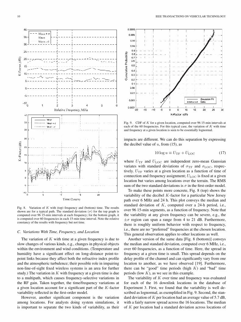
10 IEEE TRANSACTIONS ON VEHICULAR TECHNOLOGY
Fig. 8. Variation of K with (top) frequency and (bottom) time. The resultsshown are for a typical path. The standard deviation (σ) for the top graph iscomputed over 96 15-min intervals at each frequency; for the bottom graph, itis computed over 60 frequencies in each 15-min time interval. Note the relativeconstancy of the results with frequency but not time.
C. Variations With Time, Frequency, and Location
The variation of K with time at a given frequency is due toslow changes of various kinds, e.g., changes in physical objectswithin the environment and wind conditions. (Temperature andhumidity have a significant effect on long-distance point-to-point links because they affect both the refractive index profileand the atmospheric turbulence; their possible role in impairingnon-line-of-sight fixed wireless systems is an area for furtherstudy.) The variation in K with frequency at a given time is dueto a multipath, which causes frequency-selective variations inthe RF gain. Taken together, the time/frequency variations ata given location account for a significant part of the K-factorvariability reflected in the first-order model.
However, another significant component is the variationamong locations. For analysts doing system simulations, itis important to separate the two kinds of variability, as their
Fig. 9. CDF of K for a given location, computed over 96 15-min intervals ateach of the 60 frequencies. For this typical case, the variation of K with timeand frequency at a given location is seen to be essentially lognormal.
impacts are different. We can do this separation by expressingthe decibel value of u, from (15), as
10 log u ≡ UTF + ULOC (17)
where UTF and ULOC are independent zero-mean Gaussianvariates with standard deviations of σTF and σLOC, respec-tively. UTF varies at a given location as a function of time ofconnection and frequency assignment; ULOC is fixed at a givenlocation but varies among locations over the terrain. The RMSsum of the two standard deviations is σ in the first-order model.
To make these points more concrete, Fig. 8 (top) shows thevariability of the decibel K-factor for a particular New Jerseypath over 6 MHz and 24 h. This plot conveys the median andstandard deviation of K, computed over a 24-h period, i.e.,over 96 15-min segments, as a function of frequency. Note thatthe variability at any given frequency can be severe, e.g., the±σ region can span a range from 4 to 21 dB. Furthermore,there is roughly uniform behavior with respect to frequency,i.e., there are no “preferred” frequencies at the chosen location.This general observation applies to other locations as well.
Another version of the same data [Fig. 8 (bottom)] conveysthe median and standard deviation, computed over 6 MHz, i.e.,over 60 frequencies, as a function of time. Here, the spread infrequency at a given time is small. This spread depends on thedelay profile of the channel and can significantly vary from onelocation to another, as we have observed [19]. Furthermore,there can be “good” time periods (high K) and “bad” timeperiods (low K), as we see in this example.
The variability of K over time and frequency was evaluatedfor each of the 16 downlink locations in the database ofExperiment 3. First, we found that the variability is well de-scribed as lognormal, as exemplified in Fig. 9. Second, the stan-dard deviation of K per location had an average value of 5.7 dB,with a fairly narrow spread across the 16 locations. The medianof K per location had a standard deviation across locations of

GREENSTEIN et al.: RICEAN K-FACTORS IN NARROW-BAND FIXED WIRELESS CHANNELS 11
Fig. 10. Scatter plot of K-factor and wind speed for six New Jersey locations.
Fig. 11. Mean and standard deviation of the decibel K-factor as functions ofwind speed for the six New Jersey locations. The general inverse relationshipof K and wind speed is evident.
4.3 dB. The RMS sum of the two standard deviations is 7.1 dB,which we cited earlier as the global value over time, frequency,and location.
We propose that, in the lognormal model for K, 10 logu should be decomposed as in (17), with σTF = 5.7 dB andσLOC = 5.6 dB, the latter being larger than 4.3 dB to reflectour imperfect modeling of the median K (see Section IV-A).The RMS sum of the two σ’s is 8.0 dB.
D. Influence of Wind Conditions
In the long-duration path-loss measurements of Experi-ments 3 and 4, we simultaneously measured wind speed atthe base and terminal locations. The wind speed data wererecorded every second and later averaged, in offline processing,over 15-min intervals. Here, we present some illustrative resultsbased on 24-h records for each of the six New Jersey locations(a data subset of Experiment 3) and a single 48-h record
Fig. 12. Simultaneous fading observed on three fixed links in Naperville overa 48-h period.
during which fading on links to three Naperville locations weresimultaneously observed (a data subset of Experiment 4).
The observation by us and others, e.g., [6]–[9], that higherwind speeds lead to lower K-factors is consistent with thepicture of leaves, branches, and other objects moving in thewind and causing time variations in the sum of received rays. Inour results, the correlation between wind speed at the base andthe decibel K-factor was found to be −0.47; that between windspeed at the terminal and the decibel K-factor was found to be−0.56. These negative correlations are in line with our intuitiveexpectations.
Fig. 10 shows a scatter plot of K and wind speed, where theinverse correlation is in evidence. Each point is for a 15-minsegment, and there were 96 such segments at 60 frequenciesfor each of the six terminal locations. For this data set, Fig. 11shows the manner in which the mean of the K-factor (indecibels) decays with wind speed, calculated in the followingwind speed intervals (in kilometers per hour): 0 (no discerniblewind), (0, 2], (2, 4], (4, 8], and (8, 16]. The midpoint valuesof these intervals were chosen as the wind speed points on theabscissa. The steady decrease in the number of data points thatwe see at higher wind speeds makes it difficult to reliably esti-mate the standard deviation of K as a function of wind speed.Instead, we simply note that the standard deviations observedfor no discernible wind is approximately 5.5 dB and that theglobal value over all other speeds is approximately 5.2 dB.The seemingly larger spread at zero wind speed (Fig. 10) is aresult of the very large number of data points, i.e., as the numberof points increases, and so does the likelihood of seeing themore extreme low-probability values.
Fig. 12 shows the signal fading experienced over a 48-hperiod on three different non-line-of-sight paths, from a 25-m-high base station in Naperville, IL, to three residences locatedwithin a 45◦ sector at distances of 600, 1000, and 1200 m.The first two paths are each obstructed by trees and structureslocated a few hundred meters away from the remote terminal;the latter path is obstructed by a large stand of trees that islocated a few tens of meters from the remote terminal. Thesimultaneous onset of distinct fading events on the three links isclearly visible, but the depth of fading increases as the path be-comes increasingly harsh. The high correlation between fadingevents on different links within the same cell has implicationsfor radio resource management in fixed wireless systems.
12 IEEE TRANSACTIONS ON VEHICULAR TECHNOLOGY
We do not offer the partial results given here as a model forthe dependence of K upon wind speed. We merely use themto illustrate an important physical relationship. For a meaning-ful model development, considerably more experimental datawould be required.
V. CONCLUSION
We have theorized and demonstrated that narrow-band chan-nels in fixed wireless systems can be well modeled by Riceanfading, and we have shown a simple accurate way to computeRicean K-factors from time records of path gain magnitude.The K-factor is a key indicator of the severity of fading; there-fore, modeling its statistics over fixed wireless environments isessential to the study of systems using either narrow-band ormulticarrier radio techniques.
To this end, we have described the collection and reductionof a large body of data at 1.9 GHz for suburban paths in NewJersey, Illinois, and Washington. Whereas other studies havefocused on locations and scenarios in which moving vehiclesand pedestrians have a significant effect on fixed wireless links,we have focused on quiet residential areas where windblowntrees and foliage appear to have the most significant impact. Wehave developed a statistical model that presents K as lognormalover time, frequency, and user location in such environments,with the median being a simple function of season, antennaheight, antenna beamwidth, and distance. Moreover, we haveseparated the variability about the median into two parts: onedue to time and frequency variations per location and one dueto changes among locations. We have also demonstrated theconsistency of key results across different experiments. Finally,we have produced results on the relationship of the K-factorto wind conditions. The results will be useful to those engagedin the design of fixed wireless systems and/or the modeling offixed wireless channels.
ACKNOWLEDGMENT
We are indebted to numerous past and present AT&T col-leagues and contractors for collecting and processing the largequantities of path loss data used in this study. They areD. J. Barnickel, M. K. Dennison, B. J. Guarino, P. B. Guerlain,D. Jacobs, S. C. Kim, R. S. Roman, A. J. Rustako, Jr.,S. K. Wang, J. Lee, L. Roberts and M. Stephano.
REFERENCES
[1] D. Greenwood and L. Hanzo, “Characterization of mobile radio chan-nels,” in Mobile Radio Communications, R. Steele, Ed. London, U.K.:Pentech, 1992, pp. 163–185.
[2] M. Schwartz, W. R. Bennett, and S. Stein, Communication Systems andTechniques. New York: McGraw-Hill, 1966, sec. 9.2.
[3] J. D. Parsons, The Mobile Radio Propagation Channel. Hoboken, NJ:Wiley, 1992, pp. 134–136.
[4] W. C. Jakes, Jr., Ed., Microwave Mobile Communications. New York:Wiley, 1974.
[5] M. J. Gans, N. Amitay, Y. S. Yeh, T. C. Damen, R. A. Valenzuela,C. Cheon, and J. Lee, “Propagation measurements for fixed wireless loops(FWL) in a suburban region with foliage and terrain blockages,” IEEETrans. Wireless Commun., vol. 1, no. 2, pp. 302–310, Apr. 2002.
[6] E. R. Pelet, J. E. Salt, and G. Wells, “Effect of wind on foliage obstructedline-of-sight channel at 2.5 GHz,” IEEE Trans. Broadcast., vol. 50, no. 3,pp. 224–232, Sep. 2004.
[7] D. Crosby, V. S. Abhayawardhana, I. J. Wassell, M. G. Brown, andM. P. Sellars, “Time variability of the foliated fixed wireless access chan-nel at 3.5 GHz,” in Proc. IEEE VTC, May 30–Jun. 1, 2005, pp. 106–110.
[8] M. H. Hashim and S. Stavrou, “Measurements and modeling of windinfluence on radiowave propagation through vegetation,” IEEE Trans.Wireless Commun., vol. 5, no. 5, pp. 1055–1064, May 2006.
[9] H. Suzuki, C. D. Wilson, and K. Ziri-Castro, “Time variation characteris-tics of wireless broadband channel in urban area,” in Proc. 1st Eur. Conf.Antennas Propag., Nice, France, Nov. 2006.
[10] L. Ahumada, R. Feick, and R. A. Valenzuela, “Characterization of tem-poral fading in urban fixed wireless links,” IEEE Commun. Lett., vol. 10,no. 4, pp. 242–244, Apr. 2006.
[11] R. P. Torres, B. Cobo, D. Mavares, F. Medina, S. Loredo, and M. Engels,“Measurement and statistical analysis of the temporal variations of a fixedwireless link at 3.5 GHz,” Wireless Pers. Commun., vol. 37, no. 1/2,pp. 41–59, Apr. 2006.
[12] R. Feick, R. A. Valenzuela, and L. Ahumada, “Experiment results onthe level crossing rate and average fade duration for urban fixed wirelesschannels,” IEEE Trans. Commun., vol. 9, no. 1, pp. 175–179, Jan. 2007.
[13] L. J. Greenstein, S. S. Ghassemzadeh, V. Erceg, andD. G. Michelson, “Ricean K-factors in narrowband fixed wirelesschannels,” in Proc. WPMC, Amsterdam, The Netherlands, 1999.
[14] V. Erceg, “Channel models for fixed wireless applications,” IEEE802.16 Broadband Wireless Access Working Group, IEEE 802.16a-03/01,Jun. 27, 2003.
[15] L. J. Greenstein, D. G. Michelson, and V. Erceg, “Moment-methodestimation of the Ricean K-factor,” IEEE Commun. Lett., vol. 3, no. 6,pp. 175–176, Jun. 1999.
[16] C. Tepedelenlioglu, A. Abdi, and G. B. Giannakis, “The Ricean K factor:Estimation and performance analysis,” IEEE Trans. Wireless Commun.,vol. 2, no. 4, pp. 799–810, Jul. 2003.
[17] Y. Chen and N. C. Beaulieu, “Maximum likelihood estimation of the Kfactor in Ricean fading channels,” IEEE Commun. Lett., vol. 9, no. 12,pp. 1040–1042, Dec. 2005.
[18] V. Erceg, L. J. Greenstein, S. Y. Tjandra, S. R. Parkoff, A. Gupta,B. Kulic, A. A. Julius, and R. Bianchi, “An empirically based path lossmodel for wireless channels in suburban environments,” IEEE J. Sel.Areas Commun., vol. 17, no. 7, pp. 1205–1211, Jul. 1999.
[19] V. Erceg, D. G. Michelson, S. S. Ghassemzadeh, L. J. Greenstein,A. J. Rustako, Jr., P. B. Guerlain, M. K. Dennison, R. S. Roman,D. J. Barnickel, S. C. Wang, and R. R. Miller, “A model for the multipathdelay profile of fixed wireless channels,” IEEE J. Sel. Areas Commun.,vol. 17, no. 3, pp. 399–410, Mar. 1999.
[20] S. R. Hanna and J. C. Chang, “Representativeness of wind measure-ments on a mesoscale grid with station separations of 312 m to 10 km,”Boundary-Layer Meteorol., vol. 60, no. 4, pp. 309–324, Sep. 1992.
[21] M. F. Ibrahim and J. D. Parsons, “Signal strength prediction in built-upareas. Part l: Median signal strength,” Proc. Inst. Elect. Eng.—F, vol. 130,no. 5, pp. 377–384, Aug. 1983.
Larry J. Greenstein (S’59–M’67–SM’80–F’87–LF’02) received the B.S., M.S., and Ph.D. degreesin electrical engineering from the Illinois Instituteof Technology, Chicago, in 1958, 1961, and 1967,respectively.
From 1958 to 1970, he was with IIT ResearchInstitute, Chicago, working on radio frequency inter-ference and anticlutter airborne radar. He joinedBell Laboratories, Holmdel, NJ, in 1970. He waswith AT&T for 32 years, conducting research ondigital satellites, point-to-point digital radio, optical
transmission techniques, and wireless communications. For 21 years duringthat period (1979–2000), he led a research department renowned for itscontributions in these fields. He is currently a Research Scientist with theWireless Information Network Laboratory (WINLAB), Rutgers University,North Brunswick, NJ, working in the areas of ultrawideband, sensor net-works, multiple-input–multiple-output-based systems, broadband power linesystems, and radio channel modeling. He has been a Guest Editor, SeniorEditor, and Editorial Board Member for numerous publications.
Dr. Greenstein is an AT&T Fellow. He is a recipient of the IEEE Com-munications Society’s Edwin Howard Armstrong Award and a corecipient offour best paper awards. He is currently the Director of Journals for the IEEECommunications Society.

GREENSTEIN et al.: RICEAN K-FACTORS IN NARROW-BAND FIXED WIRELESS CHANNELS 13
Saeed S. Ghassemzadeh (S’88–M’91–SM’02) re-ceived the B.S., M.S., and Ph.D. degrees in electricalengineering from the City University of New York,New York, in 1989, 1991, and 1994, respectively.
From 1989 to 1992, he was with SCS Mobile-com, which is a wireless technology developmentcompany, where he conducted research in the areasof wireless channel modeling. In 1992, while work-ing toward the Ph.D. degree, he joined InterDigital,where he worked as a Principal Research Engineer,conducting research in the areas of fixed/mobile
wireless channels, and was involved in system integration and testing ofB-code-division multiple access (CDMA) technology. At the same time, hewas also an Adjunct Lecturer with the City University of New York. In1995, he joined AT&T Wireless Communication Center of Excellence, AT&TBell Laboratories, where he was involved in the design and developmentof the fixed wireless base station. He also conducted research in areas ofCDMA technologies, propagation channel measurement and modeling, satellitecommunications, wireless local area networks, and coding in wireless systems.He is currently Principal Member of Technical Staff with the CommunicationTechnology Research Department at AT&T Labs-Research, Florham Park,NJ. His current research interest includes wireless propagation measurementand modeling, cognitive radio, wireless local area networks, and terahertzcommunications.
Dr. Ghassemzadeh is a member of the IEEE Communication Society andIEEE Vehicular Technology Society. He is currently an Associate Editor for theIEEE TRANSACTIONS ON WIRELESS COMMUNICATIONS and the Journal ofCommunications and Networks.
Vinko Erceg (M’92–SM’98–F’07) received theB.Sc. degree in electrical engineering and the Ph.D.degree in electrical engineering from the City Uni-versity of New York, in 1988 and 1992, respectively.
From 1990 to 1992, he was a Lecturer with theDepartment of Electrical Engineering, City Collegeof the City University of New York. Concurrently,he was a Research Scientist with SCS Mobilecom,Port Washington, NY, working on spread-spectrumsystems for mobile communications. In 1992, hejoined AT&T Bell Laboratories. In 1996, he joined
AT&T Labs—Research as a Principal Member of Technical Staff with theWireless Communications Research Department, where he worked on signalpropagation and other projects related to the systems engineering and perfor-mance analysis of personal and mobile communication systems. From 2000 to2002, he was with Iospan Wireless Inc., San Jose, CA, as the Director of theCommunication Systems Division, working on system, propagation, deploy-ment, and performance issues of a multiple-input–multiple-output orthogonalfrequency division multiplexing communication system. He is currently aSenior Manager with the Broadcom Corporation, San Diego, CA.
David G. Michelson (S’80–M’89–SM’99) receivedthe B.A.Sc., M.A.Sc., and Ph.D. degrees in electricalengineering from the University of British Columbia(UBC), Vancouver, BC, Canada.
From 1996 to 2001, he served as a member of ajoint team from AT&T Wireless Services, Redmond,WA, and AT&T Labs—Research, Red Bank, NJ,where he was concerned with the development ofpropagation and channel models for next-generationand fixed wireless systems. The results of this workformed the basis for the propagation and channel
models later adopted by the IEEE 802.16 Working Group on Broadband FixedWireless Access Standards. From 2001 to 2002, he helped to oversee thedeployment of one of the world’s largest campus wireless local area networksat UBC while also serving as an Adjunct Professor with the Department ofElectrical and Computer Engineering. Since 2003, he has led the Radio ScienceLaboratory, Department of Electrical and Computer Engineering, UBC, wherehis current research interests include propagation and channel modeling forfixed wireless, ultra wideband, and satellite communications.
Prof. Michelson is a registered professional engineer. He serves as the Chairof the IEEE Vehicular Technology Society Technical Committee on Propaga-tion and Channel Modeling and as an Associate Editor for Mobile Channelsfor IEEE Vehicular Technology Magazine. In 2002, he served as a Guest Editorfor a pair of Special Issues of the IEEE JOURNAL ON SELECTED AREAS IN
COMMUNICATIONS concerning propagation and channel modeling. From 2001to 2007, he served as an Associate Editor for the IEEE TRANSACTIONS ON
VEHICULAR TECHNOLOGY. From 1999 to 2007, he was the Chair of the IEEEVancouver Section’s Joint Communications Chapter. Under his leadership, thechapter received Outstanding Achievement Awards from the IEEE Communi-cations Society in 2002 and 2005 and the Chapter of the Year Award from IEEEVehicular Technology Society in 2006. He received the E. F. Glass Award fromIEEE Canada in 2009.


![1 $SU VW (G +LWDFKL +HDOWKFDUH %XVLQHVV 8QLW 1 X ñ 1 … · 2020. 5. 26. · 1 1 1 1 1 x 1 1 , x _ y ] 1 1 1 1 1 1 ¢ 1 1 1 1 1 1 1 1 1 1 1 1 1 1 1 1 1 1 1 1 1 1 1 1 1 1 1 1 1 1](https://img.pdfslide.net/doc/110x75/5fbfc0fcc822f24c4706936b/1-su-vw-g-lwdfkl-hdowkfduh-xvlqhvv-8qlw-1-x-1-2020-5-26-1-1-1-1-1-x.jpg)
![1 ¢ Ù 1 £¢ 1 £ £¢ 1 - Narodowy Bank Polski · 1 à 1 1 1 1 \ 1 1 1 1 ¢ 1 1 £ 1 £ £¢ 1 ¢ 1 ¢ Ù 1 à 1 1 1 ¢ à 1 1 £ ï 1 1. £¿ï° 1 ¢ 1 £ 1 1 1 1 ] 1 1 1 1 ¢](https://img.pdfslide.net/doc/110x75/5fc6757af26c7e63a70a621e/1-1-1-1-narodowy-bank-polski-1-1-1-1-1-1-1-1-1-1-1.jpg)