S1  

Supplemental material:

Losses of ammonia and nitrate from agriculture and their effect on nitrogen recovery in the European Union and the United States between 1900 and 2050

Hans J.M van Grinsven*, Lex Bouwman, Kenneth G. Cassman, Harold M. van Es, Michelle L. McCrackin, Arthur H.W. Beusen

Pages: 20

Figures: 11

Tables: 4

S2  

Agro-environmental policies in the United Stated and the European Union

EU policies After severe food shortages in the decade after WWII, one goal of the EU Common Agricultural Policy (CAP; 1958) was to increase production of grain and livestock, which indirectly contributed to increased N fertilizers inputs in agriculture and to the import of animal feed from outside the EU (Oenema et al, 2011). Since the 1980s awareness of overproduction of agricultural products and associated negative environmental problems has led to a series of reforms, important ones being the introduction of milk quota (1984), set-aside regulations to take land out of crop production, and gradual abolishment of production subsidies for cereals, beef (1992), and sugar beet (2006). In view of the increasing global demand for dairy products, the EU will abolish the milk quota system in 2015. In 2003, it was agreed that the CAP has two pillars: market policies and rural development policies. In 2008, EU countries agreed to further modernize, simplify and streamline the CAP and remove restrictions on farming (the so-called ‘Health Check’). As a result of this evolution in policies, in 2011 73% of the 57 billion euro CAP subsidies were paid as single payments to farms, with an average of 200 euro per hectare. Of this total, 23% was allocated for rural development.

In the 1990s environmental concerns formed additional drivers of CAP reform. Cross-compliance is used to link environmental targets to the CAP reform. Cross-compliance requires farmers receiving CAP payments to also provide proof of meeting other relevant EU legislative goals. Some so-called Statutory Management Requirements for cross-compliance directly or indirectly address N inputs and include, for example, the 1991 Nitrates Directive (Oenema et al., 2011). EU environmental policy is mostly established by means of directives. These impose environmental objectives to be achieved by the Member States and provide flexibility for each member state to meet them. N loss from agriculture is mostly in the form of diffuse emissions of ammonia (NH3) and nitrous oxide (N2O) to air and of nitrate (NO3) to groundwater and surface water. Pollution of water bodies by nitrate is regulated by the Nitrates Directive (1991: Directive 91/676/EEC) with the aim of reducing water pollution caused or induced by nitrate from agricultural sources. The Nitrates Directive is the most important EU regulation for reducing environmental impacts of fertilizer and manure and for increasing REN (Van Grinsven et al., 2012). It restricts use of fertilizer and manure in situations with high risk of leaching and runoff, and it sets limits to the use of N in manure per hectare of agricultural land. Further, it promotes the concept of balanced fertilization, where inputs of N and P are in balance with plant demand and inevitable nutrient losses. Types and limits imposed by restrictions differ among member states and are partly negotiable with the European Commission. For most Northwestern EU states the national implementation of the Nitrates Directive also sets a legal limit to the total fertilizer equivalent input of N which generally is often close to agronomic recommendations for economically optimum fertilizer rates. In EU member states with strict implementation, e.g. Denmark and the Netherlands, limits on total N application in regions prone to nitrate leaching can be below the N recommendation (Van Grinsven et al., 2012).

S3  

Two other important EU directives to protect aquatic ecosystems against eutrophication are the Water Framework Directive and the Marine Strategy Framework. Different from the Nitrates Directive, these directives apply to all sources of nutrients. These directives aim at maintaining or establishing the ecological integrity of aquatic ecosystems, however without imposing restrictions on the use or losses of N from agricultural sources. In addition there are multilateral agreements to protect the marine environment of among others the North-East Atlantic (OSPAR convention, 1992) and the Baltic Sea (HELCOM convention, 2000). Protection strategies include targets and programs to reduce emission of nitrogen (and phosphorus); for OSPAR (2014) this target is a reduction of N (and P) loadings by 50% relative to 1985 levels, for HELCOM (2014) the target for N is a 13% reduction relative to 1997-2003 inputs, and 41% for P.

Emissions of NH3 are regulated by the National Emission Ceilings Directive (NEC Directive; 2001/81/EC) with the purpose of protecting the environment and human health against risks from acidification, eutrophication and ground-level ozone contamination of air quality. There is no direct relationship between the national ceilings of NH3 and N oxides (NOx) and the critical N deposition loads for ecosystems. The ceiling for NH3 is the result of political negotiations between the European Commission and member states. Total emission by the EU in 2010 was 3.6 Tg NH3,0.7 Tg below the ceiling of 4.3 Tg NH3, but four member states were exceeding their national ceiling. More recently, the UNE ECE Gothenborg revision in 2012 set the EU 2020 NH3 ceiling at 3.6 Tg, but this still must be endorsed by the European Commission (http://www.unece.org/index.php?id=29858). Large hog and poultry livestock operations, or Concentrated Animal Feeding Operations (CAFO’s) must comply with the Industrial Emissions Directive (2010; 2010/75/EU) which requires installations to apply best available techniques to control emissions.

EU policies for reduction of nitrous oxide (N2O) emissions are an integral part of the EU implementation of the Kyoto Protocol (1997-2012). Currently, a new protocol is being negotiated. A set of binding legislative acts has been put in place to ensure the EU meets its climate and energy targets. The "20-20-20" targets set three key objectives for 2020: (1) A 20% reduction in EU greenhouse gas emissions from 1990 levels; (2) Increasing the share of EU energy consumption produced from renewable resources to 20%; and (3) A 20% improvement in the EU's energy efficiency. These relative reduction targets also apply to the agricultural sector. The proposed targets set in 2014 for 2030 are a 40% reduction in EU greenhouse gas emissions and a 27% share of renewables (http://ec.europa.eu/clima/policies/2030/index_en.htm).

Unlike the US, EU policies currently do not directly address erosion and runoff of nutrients from agricultural lands, which can be a major source of loss in hilly and undulating landscapes. Especially in the eastern EU countries, past policies under centralized government planning strongly promoted the consolidation of land tracts into large fields where long slopes promote high erosion rates and associated nutrient and sediment losses to riverine systems.

S4  

US policies The history of US Farm Bills goes back to the 1920s with the Grain Futures Act that regulated trade in cereals. Soil conservation has been a national focus since the 1930’s Dust Bowl, and implementation of practices was voluntary, technically-supported by national, state and local agencies, and cost-shared at modest levels. The new Farm Bill for the period 2014-2018 passed in February 2014 and includes an annual farm budget of US$23 billion. The 2014 Farm Act includes a subsidy of US$6.1 billion per year for commodity support, US$9.8 billion for crop insurance and US$7.3 billion for conservation (US Government, 2014). Building on successes in soil conservation, much of the effort related to improved use of N on US farms occurs through voluntary adoption and incentives payments, starting in the late 1980’s. The Environmental Quality Incentives Program (EQIP), initiated in the 1996 Farm Bill, offers explicit cost-share funding or incentives payments for farmers to adopt practices that promote sound nutrient management (as written in federal and state NRCS 590 standards). These standards generally include management practices promulgated by the state land grant universities. Average payment in the US to crop farmers adopting nutrient management in EQIP in 2008 were US$22 per ha when involving only synthetic fertilizer and US$37 per ha when also involving organic waste utilization. Additional costs using manure N to replace synthetic N are estimated at US$67 per ha, which EQIP only compensates in Illinois and Indiana. (Ribaudo et al., 2011). The principal federal regulatory authority pertaining to nitrogen is derived from the 1970 Clean Air Act (CAA), the 1972 Clean Water Act (CWA), and the 1974 the Safe Drinking Water Act, and subsequent amendments. Other legislation such as the 2007 Energy Independence and Security Act (EISA), and the 1973 Endangered Species Act (ESA) contain provisions that could result in regulatory actions that affect nitrogen management. Based on authority granted to the US Environmental Protection Agency (EPA) under these legislative acts, national and regional standards are set for pollutants that have detrimental effects on human health and the environment. The EPA sets these standards for N when there is adequate scientific evidence to do so, but enforcement occurs at the state level (USEPA, 2011). EPA’s Office of Water addresses N pollution through activities such as: criteria development and standard setting, total maximum daily load (TMDL) development, National Pollution Discharge Elimination System (NPDES) permits for point N sources, watershed planning, wetlands preservation and regulation of CAFOs. Recent national assessments have found that 45% of rivers and streams, 46% of lakes, and 70% of estuaries in the US have been degraded by excess nutrients (Bricker, et al., 2007; USEPA, 2009; USEPA, 2013). For the US as a whole Alexander et al. (2007) and Seitzinger et al. (2010) estimate the relative contribution of agricultural sources to surface water loads at about 45%. For NE US this contribution is about 20% and for the Mississippi River Basin nearly 70%. Efforts to adopt nutrient water quality standards for water bodies, other than when used for drinking water, have progressed slowly and half of US states have no numeric nutrient criteria (USEPA, 2009).

In aquatic ecosystems, thresholds at which excess N becomes a problem can be expressed as a management goal such as a total maximum daily load (TMDL) or as a critical load (CL). The

S5  

TMDL should lead to an implementation plan or a watershed plan designed to meet water quality standards and restore impaired water bodies. Each state must develop TMDLs for specified lakes, reservoirs, rivers and streams, as well as protocols for developing criteria for estuaries and wetlands. The CWA does not specifically require implementation plans for TMDLs. However, it does require that waste load allocations be implemented through (NPDES) permit programs, which need to be approved by the EPA. Waste load allocation, e.g. for nitrogen, in NPDES are implemented though a wide variety of state, local, and federal programs, which may be regulatory, non-regulatory, or incentive-based, depending on the program, as well as voluntary action by citizens. There are also regional policies to reduce marine systems, like the Gulf Hypoxia Action Plan, in which the 2008 goal is a 45% reduction in riverine N and P load (Iowa State University, 2013).

Ammonia and ammonium are not regulated by the CAA. Ammonia is considered in CAFO guidelines as a water quality issue in effluent. As a result some manure management systems in CAFO’s enhance NH3 volatilization to lower the N content of manure. Only recently the resulting increase in NH3 emission into the air is viewed as a potential problem with respect to air quality concerns and N deposition. However, there is not yet a consistent view in policy on how to deal with NH3 as a potential source of atmospheric N deposition on sensitive ecosystems, of harmful PM2.5 and water acidification (USEPA, 2011). Between 1990 and 2012 emissions of NH3 from agricultural sources in the EU have decreased, while those in the US have increased (Fig. 2), which in part reflects the different policy approaches. Additional reference Oenema, O., A. Bleeker, N.A. Braathen, M. Budnáková, K. Bull, P.Cermák et al. 2011.

Nitrogen in current European policies. In: M.A. Sutton et al., editors, European Nitrogen Assessment Cambridge University Press: Cambridge, U.K., pp 612.

S6  

Short description of the IMAGE model and an extensive description of the nutrient module used for this manuscript

Selection of material copied from:

Stehfest, E., D. van Vuuren, T. Kram, L. Bouwman, R. Alkemade et al. 2014. Integrated Assessment of Global Environmental Change with IMAGE 3.0. Model description and policy applications, The Hague: PBL Netherlands Environmental Assessment Agency.

http://www.pbl.nl/sites/default/files/cms/publicaties/PBL-2014-Integrated_Assessment_of_Global_Environmental_Change_with_IMAGE_30-735.pdf

1.2 IMAGE 3.0 in a nutshell

The IMAGE suite of models, run by PBL, is a dynamic integrated assessment framework to analyse global change. IMAGE allows us to look into the future and helps to identify and map out major challenges ahead. A more balanced interaction between human development and the natural system is needed. IMAGE supports policymakers to address major transitions regarding the use of energy, land and water. The IMAGE 3.0 framework addresses a set of global environmental issues and sustainability challenges. The most prominent are climate change, land-use change, biodiversity loss, modified nutrient cycles, and water scarcity. These highly complex issues are characterised by long-term dynamics and are either global issues, such as climate change, or manifest in a similar form in many places making them global in character. Typically, these global environmental issues have emerged as human societies have harnessed natural resources to support their development, for instance to provide energy, food, water and shelter. IMAGE 3.0 is a comprehensive integrated modelling framework of interacting human and natural systems. The model framework is suited to large scale (mostly global) and long-term (up to the year 2100) assessments of interactions between human development and the natural environment, and integrates a range of sectors, ecosystems and indicators. The impacts of human activities on the natural systems and natural resources are assessed and how such impacts hamper the provision of ecosystem services to sustain human development. The model identifies socio-economic pathways, and projects the implications for energy, land, water and other natural resources, subject to resource availability and quality. Unintended side effects, such as emissions to air, water and soil, climatic change, and depletion and degradation of remaining stocks (fossil fuels, forests), are calculated and taken into account in future projections. IMAGE has been designed to be comprehensive in terms of human activities, sectors and environmental impacts, and where and how these are connected through common drivers, mutual impacts, and synergies and trade-offs. IMAGE 3.0 is the latest version of the IMAGE framework models, and has the following features: – Comprehensive and balanced integration of energy and land systems was a pioneering feature of IMAGE. Recently, other IAMs have been developed in similar directions and comprehensive IAMs are becoming more mainstream. – Coverage of all emissions by sources/sinks including natural sources/sinks makes IMAGE appropriate to provide input to bio-geochemistry models and complex Earth System Models (ESMs). – In addition to climate change, which is the primary focus of most IAMs, the IMAGE framework covers a broad range of closely interlinked dimensions. These include water availability and water quality,

S7  

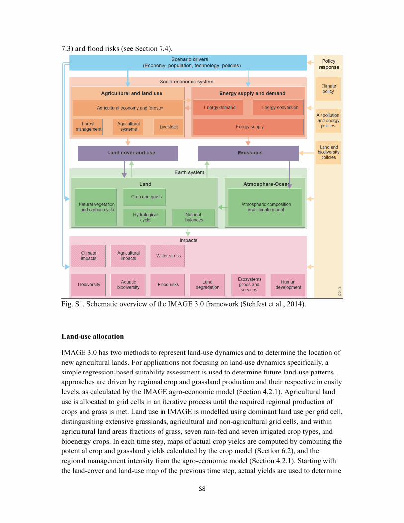
air quality, terrestrial and aquatic biodiversity, resource depletion, with competing claims on land and many ecosystem services. – Rather than averages over larger areas, spatial modelling of all terrestrial processes by means of unique and identifiable grid cells captures the influence of local conditions and yields valuable results and insights for impact models. – IMAGE is based on biophysical/technical processes, capturing the inherent constraints and limits posed by these processes and ensuring that physical relationships are not violated. – Integrated into the IMAGE framework, MAGICC 6.0 is a simple climate model calibrated to more complex climate models. Using downscaling tools, IMAGE scales global mean temperature change to spatial patterns of temperature and precipitation changes, which vary between climate models. – Detailed descriptions of technical energy systems, and integration of land-use related emissions and carbon sinks enable IMAGE to explore very low greenhouse gas emissions scenarios, contributing to the increasingly explored field of very low climate forcing scenarios. – The integrated nature of IMAGE enables linkages between climate change, other environmental concerns and human development issues to be explored, thus contributing to informed discussion on a more sustainable future including tradeoffs and synergies between stresses and possible solutions. Model components The components of the IMAGE framework are presented in Figure 1.2, which also shows the information flow from the key driving factors to the impact indicators. An overview of the model components is provided in Chapter 2, and the components are described in Chapters 3 to 8. Future pathways or scenarios depend on the assumed projections of key driving forces. Thus, all results can only be understood and interpreted in the context of the assumed future environment in which they unfold. As a result of the exogenous drivers, IMAGE projects how human activities would develop in the Human system, namely in the energy and agricultural systems (see Figure 1.2). Human activities and associated demand for ecosystem services are squared to the Earth system through the ‘interconnectors’ Land Cover and Land Use, and Emissions (see Figure 1.2). Assumed policy interventions lead to model responses, taking into account all internal interactions and feedback. Impacts in various forms arise either directly from the model, for example the extent of future land-use for agriculture and forestry, or the average global temperature increase up to 2050. Other indicators are generated by activating additional models that use output from the core IMAGE model, together with other assumptions to estimate the effects, for example, biodiversity (GLOBIO; see Sections 7.2 and

S8  

7.3) and flood risks (see Section 7.4).

Fig. S1. Schematic overview of the IMAGE 3.0 framework (Stehfest et al., 2014).

Land-use allocation

IMAGE 3.0 has two methods to represent land-use dynamics and to determine the location of new agricultural lands. For applications not focusing on land-use dynamics specifically, a simple regression-based suitability assessment is used to determine future land-use patterns. approaches are driven by regional crop and grassland production and their respective intensity levels, as calculated by the IMAGE agro-economic model (Section 4.2.1). Agricultural land use is allocated to grid cells in an iterative process until the required regional production of crops and grass is met. Land use in IMAGE is modelled using dominant land use per grid cell, distinguishing extensive grasslands, agricultural and non-agricultural grid cells, and within agricultural land areas fractions of grass, seven rain-fed and seven irrigated crop types, and bioenergy crops. In each time step, maps of actual crop yields are computed by combining the potential crop and grassland yields calculated by the crop model (Section 6.2), and the regional management intensity from the agro-economic model (Section 4.2.1). Starting with the land-cover and land-use map of the previous time step, actual yields are used to determine

S9  

crop and grassland production on current agricultural land. This is compared to the required regional crop and grassland production. If the demand exceeds calculated production, the agricultural area needs to be expanded at the cost of natural vegetation. If the calculated production of current cropland exceeds the required production, agricultural land is abandoned to adjust to the production required. Crop and grassland is either abandoned or expanded until the required production is met. Since actual yields are taken into account, changes in crop yields in time due to technological change, climate change and land heterogeneity are included. If yields in the new agricultural areas are lower than average in the current area, relatively more agricultural land is required compared to the production increase.

A grid cell is only regarded suitable for agriculture if the potential rain-fed production is at least 5% of the global maximum attainable crop yield. Grid cells with a production potential between 0.05 and 5% of the maximum attainable are still assumed suitable for extensive grassland. Irrigated areas are increased on a regional scale, prescribed by external scenario dependent assumptions, such as based on FAO (Alexandratos and Bruinsma, 2012). In each time-step, more irrigated areas are allocated in agricultural land based on the need for irrigation (the difference in rain-fed and irrigated yields), and water availability.

In agricultural areas, the fraction of specific crops is determined based on the initial fractions, and modified annually based on changes in regional demand and local crop yields. As a result, the land-use fraction of a certain crop increases when the demand for this crop increases faster than for other crops, or if the potential yield in this grid cell increases more than for other crops. Land use in IMAGE is modelled using dominant land use types per grid cell on a 0.5ox0.5o resolution. In reality, land use is more heterogeneous. Many applications require higher resolution and additional data, such as studies on biodiversity and agricultural intensification (Verburg et al., 2012).

The nutrient module

Introduction Human activity has accelerated the Earth’s biogeochemical nitrogen (N) and phosphorus (P) cycles through increasing fertiliser use in agriculture (Bouwman et al., 2013c). Increased use of N and P fertilisers has raised food production to support the rapidly growing world population, and increasing per capita consumption particularly of meat and milk (Galloway et al., 2004). The side effect is that significant proportions of the mobilised N are lost through ambient emissions of ammonia (NH3), nitrous oxide (N2O) and nitric oxide (NO). Ammonia contributes to eutrophication and acidification when deposited on land. Nitric oxide plays a role in tropospheric ozone chemistry, and nitrous oxide is a potent greenhouse gas and depleting substance of stratospheric ozone (Ravishankara et al. 2009). Moreover, large proportions of mobilised N and P in watersheds enter the groundwater through leaching, and are released to surface waters through groundwater transport and surface runoff. Subsequently, nutrients in streams and rivers are transported to coastal marine systems, reduced by retention but augmented by releases from point sources, such as sewerage systems

S10  

and industrial facilities. This has resulted in negative impacts on human health and the environment, such as groundwater pollution, loss of habitat and biodiversity, an increases in the frequency and severity of harmful algal blooms, eutrophication, hypoxia and fish kills (Diaz and Rosenberg, 2008; Zhang et al., 2010). The harmful effects of eutrophication have spread rapidly around the world, with large-scale implications for biodiversity, water quality, fisheries and recreation, in both industrialised and developing regions (UNEP, 2002). Input of nutrients in freshwater and coastal marine ecosystems also disturbs the stoichiometric balance of N, P and Si (silicon) (Rabalais, 2002) affecting total plant production and the species composition in ecosystems. To assess eutrophication as a consequence of increasing population, and economic and technological development, IMAGE 3.0 includes a nutrient model, which comprises three modules: – Wastewater module calculating nutrient flows in wastewater discharges (Figure 6.4.1, top); – Soil nutrient budget module describing all input and output of N and P in soil compartments (Figure 6.4.1, middle); – Nutrient environmental fate describing the fate of soil nutrient surpluses and wastewater nutrients in the aquatic environment (Figure 6.4.1, bottom).

Soil nutrient budget The soil budget approach (Bouwman et al., 2009; Bouwman et al., 2013c) considers all N and P inputs and outputs for IMAGE grid cells. N input terms in the budgets include application of synthetic N fertiliser (Nfert) and animal manure (Nman), biological N fixation (Nfix), and atmospheric N deposition (Ndep). Output terms include N withdrawal from the field through crop harvesting, hay and grass cutting, and grass consumed by grazing animals (Nwithdr).

The soil N budget (Nbudget) is calculated as follows:

N-budget = Nfert + Nman + Nfix + Ndep − Nwithdr

The same approach is used for P, with input terms being animal manure and fertiliser. The soil nutrient budget does not include nutrient accumulation in soil organic matter for a positive budget (surplus), or nutrient depletion due to soil organic matter decomposition and mineralisation. With no accumulation, a surplus represents a potential loss to the environment. For N this includes NH3 volatilisation (see Section 5.2), denitrification, surface runoff and leaching. For P, this is surface runoff. For spatial allocation of the nutrient input to IMAGE grid cells, grass and the crop groups in IMAGE (temperate cereals, rice, maize, tropical cereals, pulses, roots and tubers, oil crops, other crops, energy crops) and grass are aggregated to five broad groups. These groups are grass, wetland rice, leguminous crops, other upland crops and energy crops for both mixed and pastoral production systems (see Section 4.2.4).

S11  

Fig. S2. Schematic overview of the IMAGE global nutrient model (Beusen et al., 2014, adapted from Stehfest et al., 2014).

Fertiliser: Fertiliser use is based on nutrient use efficiency, representing crop production in kilograms of dry matter per kilogram of fertiliser N (NUE) and P (PUE). NUE and PUE vary between countries because of differences in crop mix, attainable yield potential, soil quality, amount and form of N and P application and management. In constructing scenarios on fertiliser use, data on the 1970–2005 period serve as a guide to distinguish countries with an input exceeding crop uptake (positive budget or surplus) from countries with a deficit. Generally, farmers in countries with a surplus are assumed to be increasingly efficient in fertiliser use (increasing NUE and PUE). In countries with nutrient deficits, an increase in crop yields is only possible with an increase in the nutrient input. Initially, this will lead to

S12  

decreasing NUE and PUE, showing a decrease in soil nutrient depletion due to increased fertiliser use.

Manure: Total manure production is computed from animal stocks and N and P excretion rates (Figure 6.4.1, middle). IMAGE uses constant N and P excretion rates per head for dairy and non-dairy cattle, buffaloes, sheep and goats, pigs, poultry, horses, asses, mules and camels. Constant excretion rates imply that the N and P excretion per unit of product decreases with increased milk and meat production per animal. N and P in the manure for each animal category are spatially allocated to mixed and pastoral systems. In each country and system, the manure is distributed over three management systems: grazing; storage in animal housing and storage systems; and manure used outside the agricultural system for fuel or other purposes. The quantity of manure assigned to grazing is based on the proportion of grass in feed rations (Figure 6.4.1, middle). Stored animal manure available for cropland and grassland application includes all stored and collected manure, excluding ammonia volatilisation from animal houses and storage systems. In general, IMAGE assumes that 50% of available animal manure from storage systems is applied to arable land and the rest to grassland in industrialised countries. In most developing countries, 95% of the available manure is spread on croplands and 5% on grassland, thus accounting for the lower economic importance of grass compared to crops in these countries. In the European Union, maximum manure application rates are 170 to 250 kg N per ha, reflecting current regulations.

Biological N2 fixation: Data on biological N2 fixation by leguminous crops (pulses and soybeans) are obtained from the N in the harvested product (see nutrient withdrawal) following the approach of Salvagiotti et al. (2008). Thus any change in the rate of biological N2 fixation by legumes is the result of yield changes for pulses and soybeans. In addition to leguminous crops, IMAGE uses an annual rate of biological N2 fixation of 5 kg N per ha for non-leguminous crops and grass, and 25 kg N per ha for wetland rice. N fixation rates in natural ecosystems were based on the low estimates for areal coverage by legumes (Cleveland et al., 1999) as described by Bouwman et al. (2013a).

Atmospheric deposition: Deposition rates for historical and future years are calculated by scaling a N deposition map for 2000 (obtained from atmospheric chemistry transport models), using emission inventories for the historical period and N gas emissions in the scenario considered. IMAGE does not include atmospheric P deposition.

Nutrient withdrawal: Withdrawal of N and P in harvested products is calculated from regional crop production in IMAGE and the N and P content for each crop, which is aggregated to the broad crop categories (wetland rice, leguminous crops, upland crops and energy crops). IMAGE also accounts for uptake by fodder crops. N withdrawal through grass consumption and harvest is assumed to amount to 60% of all N input (manure, fertiliser, deposition, N fixation), excluding NH3 volatilisation. P withdrawal through grazing or grass cutting is calculated as a proportion of 87.5% of fertiliser and manure P input. The rest is assumed to be lost through surface runoff. In calculating spatially explicit nutrient withdrawal, a procedure is used to downscale regional crop production data from IMAGE to country estimates for nutrient withdrawal based on distributions in 2005.

S13  

Nutrient environmental fate Nutrient losses from the plant-soil system to the soil-hydrology system are calculated from the soil nutrient budgets (Bouwman et al., 2013a). For N, the budget is corrected for ammonia volatilisation from grazing animals and from fertiliser and manure spreading (see Section 5.2, Emissions). P not taken up by plants is generally bound to soil particles, with the only loss pathway being surface runoff. N is more mobile and is transported via surface runoff and through soil, groundwater and riparian zones to surface water.

Soil denitrification and leaching: Denitrification is calculated as a proportion of the soil N budget surplus based on the effect of temperature and residence time of water and nitrate in the root zone, and the effects of soil texture, soil drainage and soil organic carbon content. In a soil budget deficit, IMAGE assumes that denitrification does not occur. Leaching is the complement of the soil N budget.

Groundwater transport, surface runoff and denitrification: Two groundwater subsystems are distinguished. One is the shallow groundwater system representing interflow and surface runoff for the upper 5 m of the saturated zone, with short travel times for the water to enter local surface water at short distances or to infiltrate the deep groundwater system. The other is the deep system with a thickness of 50 m with generally long travel times draining to larger streams and rivers. Deep groundwater is assumed to be absent in areas of non-permeable, consolidated rocks or in the presence of surface water. Denitrification during groundwater transport is based on the travel time and the half-life of nitrate. The half-life depends on the lithological class (1 year for schists and shales containing pyrite, 2 years for alluvial material, and 5 years for all other lithological classes). Flows of water and nitrate from shallow groundwater to riparian zones are assumed to be absent in areas with surface water bodies, where the flow is assumed to bypass riparian zones flowing directly to streams or rivers.

Denitrification in riparian areas: The calculation of denitrification in riparian areas is similar to that in soils, but with two differences: a biologically active layer of 0.3 m thickness is assumed instead of 1 m for other soils; and the approach includes the effect of pH on denitrification.

In-stream nutrient retention: The water that enters streams and rivers through surface runoff and discharges from groundwater and riparian zones is routed through stream and river channels, and passes through lakes, wetlands and reservoirs. The nutrient retention in each of these systems is calculated on the basis of the nutrient spiralling ecological concept, which is based on residence time and temperature as described in (Beusen et al., submitted).

Data, uncertainties and limitations

Data The data stem from various parts of IMAGE, such as land cover, biomes, crop production and allocation, livestock, fertiliser use and nutrient excretion rates. Environmental data include temperature and precipitation, runoff, and soil properties. External data are used in determining historical N excretion rates, manure spreading and fertiliser use efficiency, but their development in the future is a scenario assumption. Additional information used only in

S14  

this section includes lithology, relief and slope of the terrain. Additional data used in the nutrient budget model include subnational data as used for the United States, India, Brazil and China.

Uncertainties With regard to uncertainties, the budget calculations and individual input terms for 2000 have been found to be in close agreement (Bouwman et al., 2009) with detailed country estimates for the member countries of the Organisation for Economic Cooperation and Development (OECD, 2012). However, uncertainty is larger for some budget terms than for others. Data on fertiliser use are more reliable than on N and P animal excretions, which are calculated from livestock data (FAO, 2012a) and excretion rates per animal category. Data on crop nutrient withdrawal are less certain than on crop production, because the withdrawal is calculated with fixed global nutrient contents of the harvested proportions of marketed crops. In addition to uncertainty in nutrient contents, major uncertainties arise from insufficient data, for instance, on crops that are not marketed and on the use of crop residues. This leads to major uncertainties about nutrient withdrawal. Sensitivity analysis (Beusen et al., 2008) has shown that the main determinants of the uncertainty in the nutrient model are N excretion rates; NH3 emission rates from manure in animal housing and storage systems; the proportion of time that ruminants graze, the proportion of non-agricultural use of manure in mixed and industrial systems; and animal stocks.

S15  

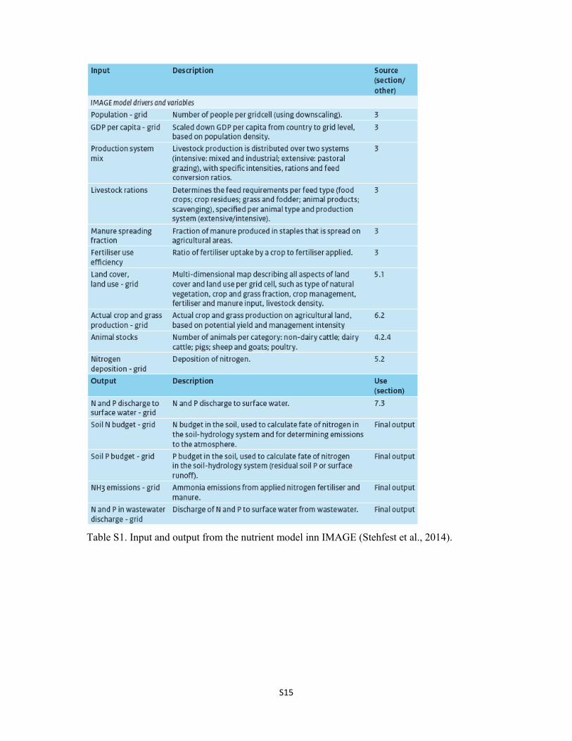
Table S1. Input and output from the nutrient model inn IMAGE (Stehfest et al., 2014).

S16  

References

Selection of peer reviewed publications since 2000 about concepts and applications of the IMAGE model focusing on agriculture and nutrients.

Beusen AHW, Bouwman AF, Heuberger PSC, Van Drecht G and Van Der Hoek KW. (2008). Bottom-up uncertainty estimates of global ammonia emissions from global agricultural production systems. Atmospheric Environment 42(24), pp. 6067–6077.

Beusen AHW, Van Beek LPH, Bouwman AF and Middelburg JJ. (submitted). Exploring changes in nitrogen and phosphorus biogeochemistry in global rivers in the twentieth century. Global Biogeochemical Cycles.

Bouwman AF, Van Vuuren DP, Derwent RG and Posch M. (2002b). A global analysis of acidification and eutrophication of terrestrial ecosystems. Water Air Soil Pollution 141, pp. 349–382.

Bouwman AF, Van der Hoek KW, Eickhout B and Soenario I. (2005). Exploring changes in world ruminant production systems. Agricultural Systems 84(2), pp. 121–153, DOI: 10.1016 j.agsy 2004.05.006.

Bouwman AF, van der Hoek KW, Van Drecht G and Eickhout B. (2006). World livestock and crop production systems, land use and environment between 1970 and 2030. In: F. Brouwer and B. McCarl (eds.), Rural Lands, Agriculture and Climate beyond 2015: A new perspective on future land use patterns. Springer, Dordrecht, pp. 75–89.

Bouwman AF, Beusen AHW and Billen G. (2009). Human alteration of the global nitrogen and phosphorus soil balances for the period 1970–2050. Global Biogeochemical Cycles 23, DOI: 10.1029/2009GB003576.

Bouwman AF, G Van Drecht, JM Knoop, AHW Beusen, CR Meinardi (2005). Exploring changes in river nitrogen export to the world's oceans. Global Biogeochemical Cycles,

Bouwman AF, Pawłowski M, Liu C, Beusen AHW, Shumway SE, Glibert PM and Overbeek CC. (2011). Global Hindcasts and Future Projections of Coastal Nitrogen and Phosphorus Loads Due to Shellfish and Seaweed Aquaculture. Reviews in Fisheries Science 19(4), pp. 331–357, DOI: 10.1080/10641262.2011.603849.

Bouwman AF, Beusen AHW, Griffioen J, Van Groenigen JW, Hefting MM, Oenema O, Van Puijenbroek PJTM, Seitzinger S, Slomp CP and Stehfest E. (2013a). Global trends and uncertainties in terrestrial denitrification and N2O emissions. Philosophical Transactions of the Royal Society B: Biological Sciences 368(1621), DOI: 10.1098/rstb.2013.0112.

Bouwman AF, Beusen AHW, Overbeek CC, Bureau DP, Pawlowski M and Glibert PM. (2013b). Hindcasts and Future Projections of Global Inland and Coastal Nitrogen and Phosphorus Loads Due to Finfish Aquaculture. Reviews in Fisheries Science 21(2), pp. 112–156, DOI: 10.1080/10641262.2013.790340.

S17  

Bouwman AF, Klein Goldewijk K, Van der Hoek KW, Beusen AHW, Van Vuuren DP, Willems WJ, Rufinoe MC and Stehfest E. (2013c). Exploring global changes in nitrogen and phosphorus cycles in agriculture induced by livestock production over the 1900– 2050 period. Proceedings of the National Academy of Sciences of the United States of America (PNAS) 110, pp. 20882–20887, DOI: 20810.21073/pnas.1012878108.

Eickhout B, A.F. Bouwman and H. van Zeijts (2006). The role of nitrogen in world food production and environmental sustainability. Agriculture, Ecosystems and Environment 116: 4-14.

Eickhout B, Van Meijl H, Tabeau A and Van Rheenen R. (2007). Economic and ecological consequences of four European land use scenarios. Land Use Policy 24(3), pp. 562–575.

Morée AL, Beusen AHW, Bouwman AF and Willems WJ. (2013). Exploring global nitrogen and phosphorus flows in urban wastes during the twentieth century. Global Biogeochemical Cycles 27, pp. 1–11, DOI: 10.1002/gbc.20072.

Sattari, S. Z., Bouwman, A. F., Giller, K. E., and Van Ittersum, M. K. (2012). Residual soil phosphorus as the missing piece in the global phosphorus crisis puzzle. Proceedings of the National Academy of Sciences of the United States of America 109, 6348‐6353.

Sattari, S. Z., van Ittersum, M. K., Giller, K. E., Zhang, F., & Bouwman, A. F. (2014). Key role of China and its agriculture in global sustainable phosphorus management. Environmental Research Letters, 9(5), 054003.

Stehfest E, Bouwman L, Van Vuuren DP, Den Elzen MGJ, Eickhout B and Kabat P. (2009). Climate benefits of changing diet. Climatic Change 95(1-2), pp. 83–102.

Stehfest E, Berg M, Woltjer G, Msangi S and Westhoek H. (2013). Options to reduce the environmental effects of livestock production - Comparison of two economic models. Agricultural Systems 114, pp. 38–53.

G Van Drecht, AF Bouwman, JM Knoop, AHW Beusen, CR Meinardi. 2003. Global modeling of the fate of nitrogen from point and nonpoint sources in soils, groundwater, and surface water. Global Biogeochemical Cycles 17.

Van Drecht G, Bouwman AF, Harrison J and Knoop JM. (2009). Global nitrogen and phosphate in urban waste water for the period 1970-2050. Global Biogeochemical Cycles 23, pp. GB0403, DOI: 10.1029/2009GB003458.

Van Minnen JG, Klein Goldewijk K, Stehfest E, Eickhout B, Drecht G and Leemans R. (2009). The importance of three centuries of land-use change for the global and regional terrestrial carbon cycle. Climatic Change 97(1-2), pp. 123–144, DOI: 10.1007/ s10584-009-9596-0.

S18 

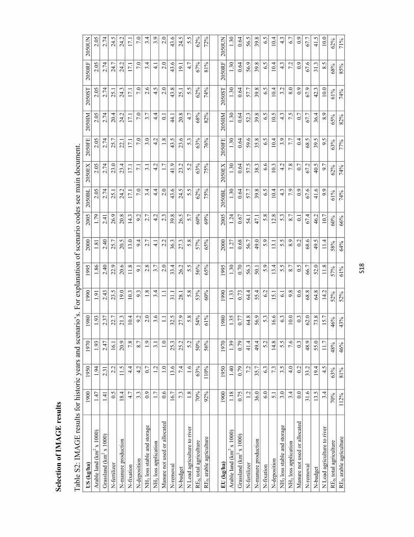
 Sel

ecti

on o

f IM

AG

E r

esu

lts

Tab

le S

2: I

MA

GE

res

ults

for

his

tori

c ye

ars

and

scen

ario

’s. F

or e

xpla

nati

on o

f sc

enar

io c

odes

see

mai

n do

cum

ent.

US

(kg/

ha)

19

00

1950

1970

1980

1990

1995

2000

2005

20

50B

L20

50E

X20

50FE

2050

IM20

50ST

2050

RF

2050

UN

Ara

ble

land

(km

2 x 1

000)

1.

47

1.94

1.93

1.93

1.91

1.86

1.81

1.79

2.

052.

052.

052.

052.

052.

052.

05

Gra

ssla

nd (

km2 x

100

0)

1.41

2.

312.

472.

372.

432.

402.

402.

41

2.74

2.74

2.74

2.74

2.74

2.74

2.74

N-f

erti

lizer

0.

5 2.

216

.122

.723

.522

.925

.726

.9

25.1

23.0

25.7

20.4

25.1

24.7

24.5

N-m

anur

e pr

oduc

tion

18.4

11

.520

.921

.319

.020

.620

.520

.8

24.2

23.4

22.1

24.2

24.3

24.2

24.2

N-f

ixat

ion

4.7

4.4

7.8

10.4

10.3

11.8

13.0

14.3

17

.117

.117

.117

.117

.117

.117

.1

N-d

epos

itio

n 3.

3 4.

28.

79.

29.

39.

19.

49.

2 7.

07.

17.

07.

07.

07.

07.

0

NH

3 lo

ss s

tabl

e an

d st

orag

e 0.

9 0.

71.

92.

01.

82.

82.

72.

7 3.

43.

13.

03.

72.

63.

43.

4

NH

3 lo

ss a

ppli

catio

n 1.

7 1.

23.

13.

63.

43.

74.

14.

2 4.

44.

24.

24.

44.

54.

13.

9

Man

ure

not u

sed

or a

lloca

ted

0.6

1.0

1.0

1.1

1.1

2.0

2.2

2.3

2.0

1.7

1.8

0.1

2.0

2.0

2.0

N-r

emov

al

16.7

13

.625

.332

.531

.133

.436

.339

.8

43.6

41.9

43.5

44.1

43.8

43.6

43.6

N-b

udge

t 7.

3 7.

425

.227

.928

.126

.227

.326

.5

24.5

23.2

23.6

20.8

25.1

19.1

24.5

N L

oad

agri

cult

ure

to r

iver

1.

8 1.

65.

25.

85.

85.

55.

85.

7 5.

55.

25.

34.

75.

54.

75.

5

RE

N to

tal a

gric

ultu

re

70%

63

%50

%54

%53

%56

%57

%60

%

62%

63%

63%

68%

62%

67%

62%

RE

N a

rabl

e ag

ricu

lture

92

%

110%

56%

61%

60%

65%

65%

69%

75

%75

%76

%82

%74

%81

%72

%

EU

(kg

/ha)

19

00

1950

1970

1980

1990

1995

2000

2005

20

50B

L20

50E

X20

50FE

2050

IM20

50ST

2050

RF

2050

UN

Ara

ble

land

(km

2 x 1

000)

1.

18

1.40

1.39

1.35

1.33

1.30

1.27

1.24

1.

301.

301.

301.

301.

301.

301.

30

Gra

ssla

nd (

km2 x

100

0)

0.75

0.

790.

790.

770.

730.

700.

680.

67

0.64

0.64

0.64

0.64

0.64

0.64

0.64

N-f

erti

lizer

1.

2 7.

241

.464

.864

.456

.356

.754

.1

57.7

57.5

59.6

52.3

57.7

56.9

56.5

N-m

anur

e pr

oduc

tion

36.0

35

.749

.456

.955

.450

.149

.047

.1

39.8

38.3

35.8

39.8

39.8

39.8

39.8

N-f

ixat

ion

6.0

6.3

5.2

5.3

6.2

5.9

5.9

5.8

6.5

6.6

6.5

6.5

6.5

6.5

6.5

N-d

epos

itio

n 5.

1 7.

314

.816

.615

.113

.413

.112

.8

10.4

10.3

10.4

10.5

10.4

10.4

10.4

NH

3 lo

ss s

tabl

e an

d st

orag

e 3.

0 3.

55.

56.

36.

15.

55.

55.

3 4.

34.

23.

94.

33.

24.

34.

3

NH

3 lo

ss a

ppli

catio

n 3.

4 4.

07.

610

.09.

88.

78.

98.

7 7.

97.

87.

77.

58.

07.

26.

7

Man

ure

not u

sed

or a

lloca

ted

0.0

0.2

0.3

0.3

0.6

0.5

0.2

0.1

0.9

0.7

0.4

0.7

0.9

0.9

0.9

N-r

emov

al

31.6

33

.248

.962

.068

.866

.768

.667

.4

67.6

67.2

68.5

67.7

67.9

67.6

67.7

N-b

udge

t 13

.5

19.4

55.0

73.8

64.8

52.0

49.5

46.2

41

.640

.539

.536

.442

.331

.341

.5

N L

oad

agri

cult

ure

to r

iver

3.

4 4.

511

.715

.714

.211

.811

.410

.7

9.9

9.7

9.5

8.9

10.0

8.5

10.0

RE

N to

tal a

gric

ultu

re

70%

63

%

48%

46

%

52%

57

%

58%

60

%

61%

62

%

63%

65

%

61%

68

%

62%

RE

N a

rabl

e ag

ricu

lture

11

2%

81%

46

%

43%

52

%

61%

64

%

66%

74

%

74%

77

%

82%

74

%

85%

71

%

 

S19  

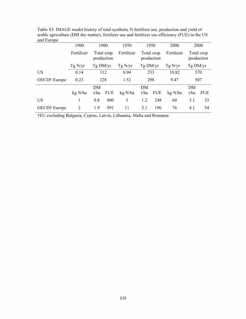
Table S3. IMAGE model history of total synthetic N fertilizer use, production and yield of arable agriculture (DM dry matter), fertilizer use and fertilizer use efficiency (FUE) in the US and Europe. 1900 1900 1950 1950 2000 2000

Fertilizer Total crop production

Fertilizer Total crop production

Fertilizer Total crop production

Tg N/yr Tg DM/yr Tg N/yr Tg DM/yr Tg N/yr Tg DM/yr

US 0.14 112 0.94 233 10.82 570

OECD† Europe 0.23 228 1.52 298 9.47 507

kg N/ha DM t/ha FUE kg N/ha

DM t/ha FUE kg N/ha

DM t/ha FUE

US 1 0.8 800 5 1.2 248 60 3.1 53

OECD† Europe 2 1.9 991 11 2.1 196 76 4.1 54

†EU excluding Bulgaria, Cyprus, Latvia, Lithuania, Malta and Romania.

S20  

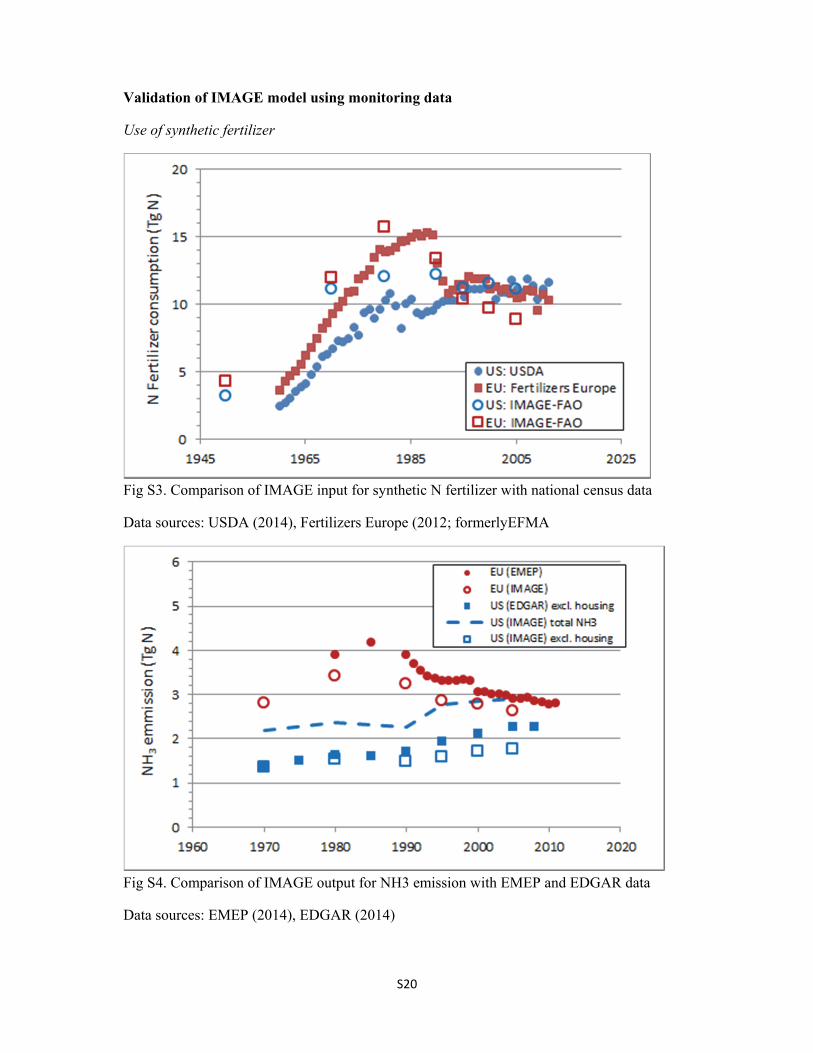
Validation of IMAGE model using monitoring data

Use of synthetic fertilizer

Fig S3. Comparison of IMAGE input for synthetic N fertilizer with national census data

Data sources: USDA (2014), Fertilizers Europe (2012; formerlyEFMA

Fig S4. Comparison of IMAGE output for NH3 emission with EMEP and EDGAR data

Data sources: EMEP (2014), EDGAR (2014)

S21  

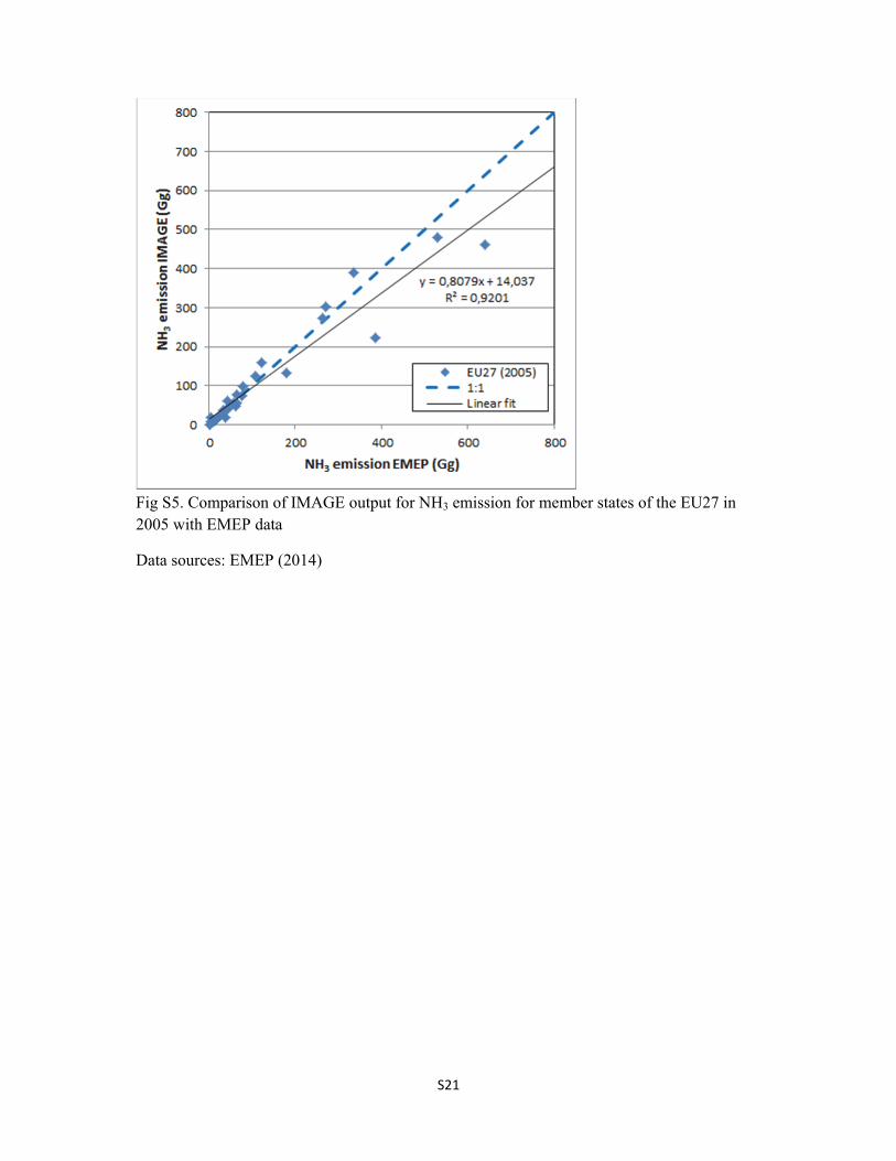
Fig S5. Comparison of IMAGE output for NH3 emission for member states of the EU27 in 2005 with EMEP data

Data sources: EMEP (2014)

S22  

Nitrogen budget agricultural land

Fig. S6. Comparison of IMAGE output for the N budget for arable agriculture in the US with IPNI data. Data sources: Fixen et al., (2012; IPNI)

Fig. S7. Comparison of IMAGE output for the N budget for total agriculture in the EU27 with cumulative national census data in Eurostat. Data sources: Eurostat (2012); gross soil N budget corrected to net soil N budget by subtraction of NH3 emission from EMEP (2012)

S23  

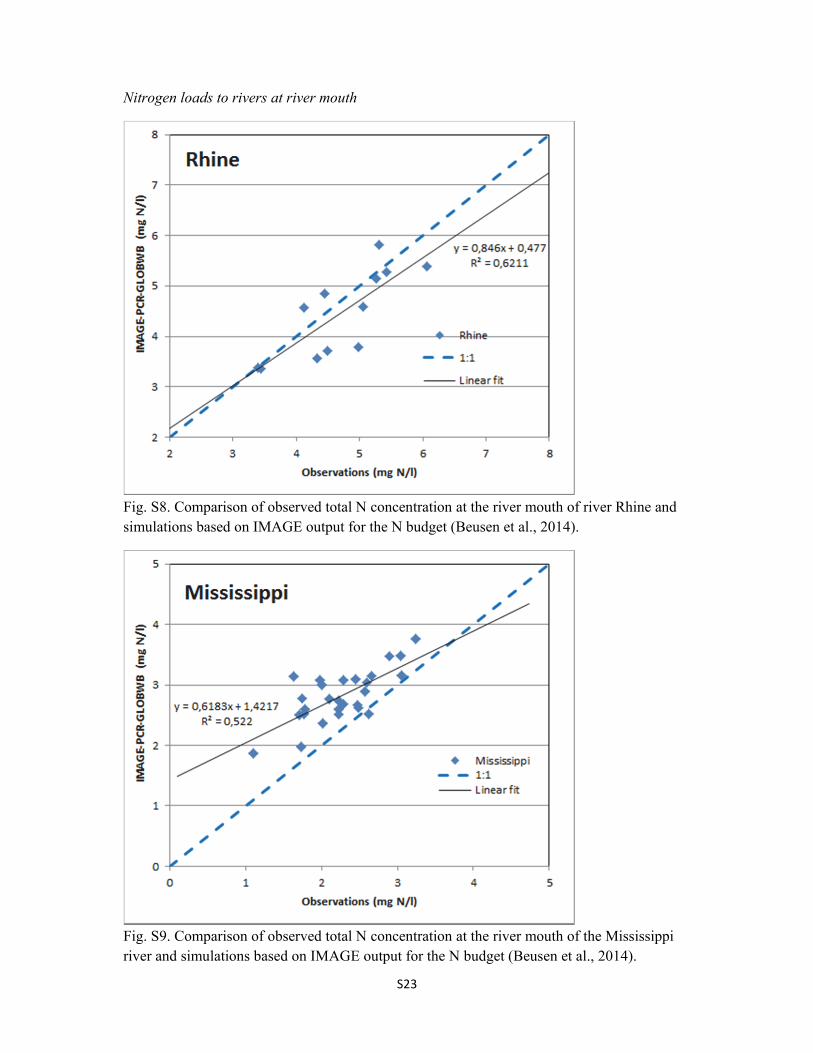
Nitrogen loads to rivers at river mouth

Fig. S8. Comparison of observed total N concentration at the river mouth of river Rhine and simulations based on IMAGE output for the N budget (Beusen et al., 2014).

Fig. S9. Comparison of observed total N concentration at the river mouth of the Mississippi river and simulations based on IMAGE output for the N budget (Beusen et al., 2014).

S24  

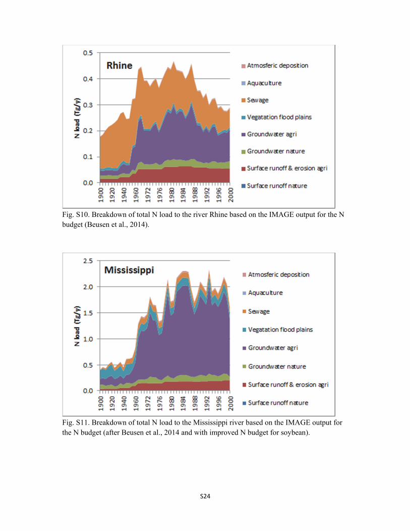
Fig. S10. Breakdown of total N load to the river Rhine based on the IMAGE output for the N budget (Beusen et al., 2014).

Fig. S11. Breakdown of total N load to the Mississippi river based on the IMAGE output for the N budget (after Beusen et al., 2014 and with improved N budget for soybean).

S25  

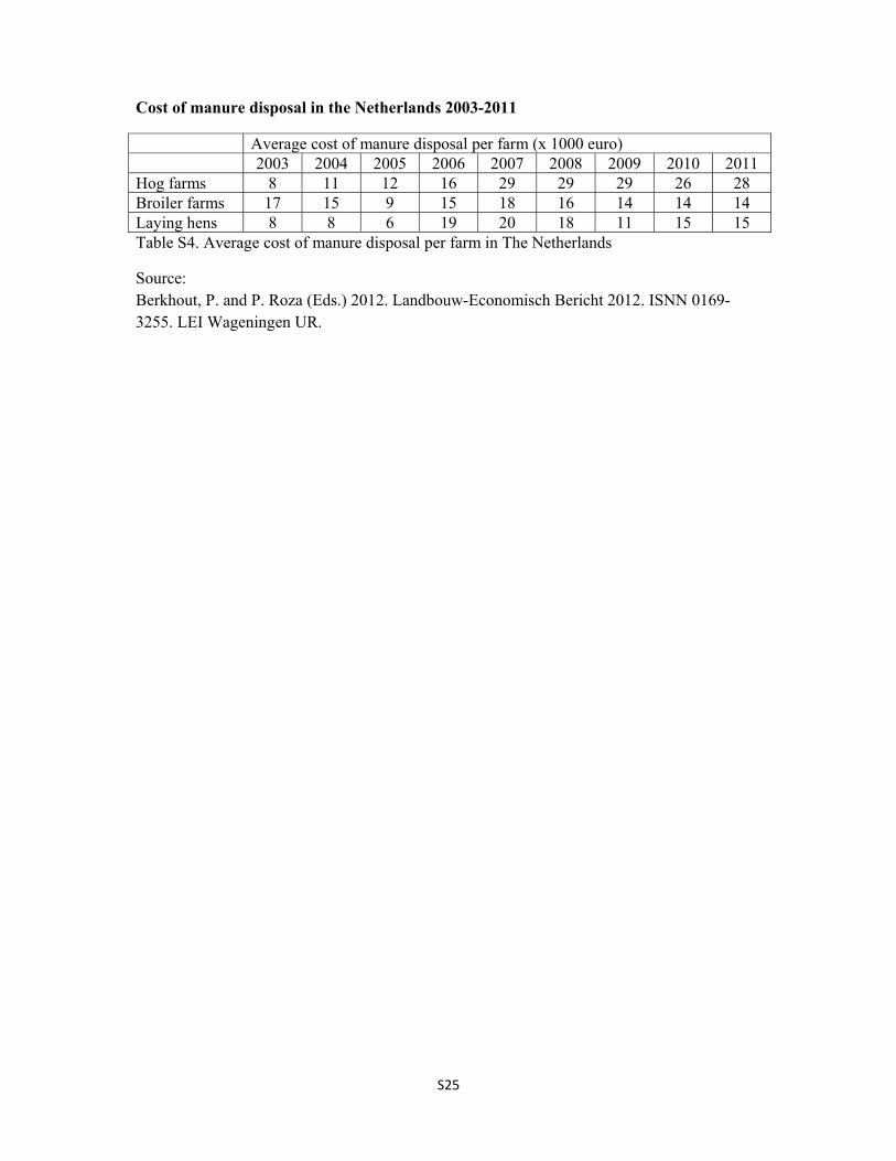
Cost of manure disposal in the Netherlands 2003-2011

Average cost of manure disposal per farm (x 1000 euro) 2003 2004 2005 2006 2007 2008 2009 2010 2011 Hog farms 8 11 12 16 29 29 29 26 28 Broiler farms 17 15 9 15 18 16 14 14 14 Laying hens 8 8 6 19 20 18 11 15 15 Table S4. Average cost of manure disposal per farm in The Netherlands

Source: Berkhout, P. and P. Roza (Eds.) 2012. Landbouw-Economisch Bericht 2012. ISNN 0169-3255. LEI Wageningen UR.