Ground-Coupled Heat Transfer Test Cases as ranking ... · PDF fileGround-Coupled Heat Transfer Test Cases as ranking simulation software ... SolidWorks Flow Simulation, Software validation,

Ground-Coupled Heat Transfer Test Cases as ranking simulationsoftware

Stanislav Sehnalek, Martin Zalesak, Jiri Vincenec, Michal Oplustil, Pavel ChrobakTomas Bata University in ZlinFaculty of Applied InformaticsNad Stranemi 4511,760 05 Zlin

Czech [email protected]

Abstract: In the present work is International European Agency Building Energy Simulation Test Task 34 used asvalidation for SolidWorks Flow Simulation 2012. IEA BESTEST methodology is based on analytical verificationof one model and on comparative validation of the rest of models. For appraisal was chosen 12 cases where halfhave stationary character and the remain half is periodical. In the beginning of the presented paper are describedcases with appropriate application. The outcome of simulation follows with discussion about results which aresegregated in the manner of periodic or steady character. The paper is wind up with outline of future research.

Key–Words: Heat transfer, Finite Element Method, SolidWorks Flow Simulation, Software validation, Benchmark,Building simulation.

1 Introduction

Share of glass used in faades of buildings is logarith-mically increasing during the last two centuries. Thisresults from some valuable features of glass, whichare transparency, low weight and ability to separatedifferent environments. Since Le Corbusiers era, glassis becoming dominant in usage for faades at the ex-pense of conventional materials. This fact could proveScheerbarts paraphrased words Bricks are only goodto hurt. In the way of usage of glass for faades thereis one important issue, which should be always takeninto account. Temperature gains caused by internaland external heat sources. These gains affect comfortof people inside these plant house buildings. A long-term research of peoples comfort in 26 office build-ings in five European Union countries was executedby [1]. Interior comfort can be provided by ventilationsystems, by shading systems or by their combination,which are not always energetically sustainable. In re-cent years, there is a particular interest in sustainabil-ity of buildings [2] and [3]. Currently, there has beengrowing interest in lowering energy performance ofbuildings. This effort is also reflected in a new Eu-ropean directive, which instructs to construct near tozero energy sufficient buildings since year 2020. Re-gardless of our experience and knowledge, there arealways a risks of constructing an inconvenient build-ing. To prevent this, appropriate design of buildingshould be achieved. Thermal properties of a build-ing could be calculated in a development phase, but

it is limited to one-dimensional and rarely as two-dimensional problem solutions thanks to the complex-ity of buildings and the mathematical apparatus avail-able. As a result of computational power increasein last decades, it is possible to design a model andimplement mathematical simulation of thermal be-haviour of a building also in three-dimensional space[4]. For such mathematical simulation it is used fi-nite element method (FEM) [5]. Thanks to the ex-panding performance of computers, FEM is used forpartial differential equations solutions as a convenientway to validate building’s behaviour [6]. However,first of all it is important to validate thermal simula-tion programs (DTSP) [7], which is used. The solu-tion can be achieved by several ways. Judkoff andNeymark developed a methodology for such intentionin the middle of 90s by [8]. Their approach is basedon the analytical solution for steady-state heat flowthrough the floor slab. Although it was developed byDelsante, Stokes and Walsh [9], although this problemhas been in focus of researchers for some time [10].It is worth to mention a simplified model by Ameri-can Society of Heating, Refrigerating and Air Condi-tioning Engineers (ASHRAE), which calculates slab-on-grade perimeter heat-loss, operates with perimeterlength and an F-factor heat loss coefficient. Delsante’smethodology focuses only on heat flow through floorslab and omits above grade constructions. Stan-dard established by ASHRAE improved Judkoff’s andNeymark’s methodology by adding cases which focus

WSEAS TRANSACTIONS on INFORMATION SCIENCE and APPLICATIONSStanislav Sehnalek, Martin Zalesak,

Jiri Vincenec, Michal Oplustil, Pavel Chrobak

E-ISSN: 2224-3402 11 Volume 12, 2015

mainly on above grade constructions and solar radia-tion [10], [11].

All mentioned methods and standards are basedon finite element analysis (FEA). In this paper, an ap-plication of International European Agency BuildingEnergy Simulation Test (IAE BESTEST) Task 34 isdescribed on SolidWorks Flow Simulation (SW-FS).This task is already approved on DTSP like are TRN-SYS, Fluent, EnergyPlus and ESP-r/BASESIMP. Be-sides that, investigation of COMSOL Multiphysicson Task 34 was done by Gerlich [12]. In the sec-tion methods is included outline of 6 cases from IAEBESTEST Task 34 along with a description of SW-FS. This chapter is followed by results section withdescription of implementation of cases on SW-FS andfinally with results from simulation. Article is sum-marized by conclusion section with discussion aboutresults which are segregated in the manner of periodicor steady character. The paper is concluded with out-line of further research.

2 Methods

This section of the paper cover several topics and isdivided in two parts. At the beginning of the section,Ground Coupling In-Depth Diagnostic Cases is de-scribed. More specifically: geometry, physical prop-erties, initial conditions and boundary conditions. Inthe second section the outline capabilities of Solid-Works Flow Simulation 2012 SP5 (SW-FS) is listed.

2.1 IEA BESTEST cases

International Energy Agency Building Energy Simu-lation Test methodology was developed by [8] in themiddle of 90’s. Combination of empirical validation,analytical verification and comparative analysis tech-niques are main proceedings of this methodology. Itoperates only with slab-on-grade heat transfer and be-came a stepping-stone for the other approaches, suchas ANSI/ASHRAE Standard 140 improved adaptationdeveloped by ASHRAE accordingly with AmericanNational Standards Institute (ANSI).

Methodology describes 17 cases of ground-coupled heat transfers designed to be compared withverified whole-building energy simulation software.Several of those already tested by IEA are EnergyPlus,FLUENT, Matlab, TRNSys and GHT. The first case,GC10a has its base in analytical solution and it is thesimplest one of all cases. Furthermore, these cases aresubdivided into three series, each with its own specifi-cation. For this paper was chosen 12 cases where firsthalf is steady-state and the rest is steady-periodic.

Figure 1: Elevation section (Neymark and Judkoff,2008)

• Series a

– The main purpose of this series is to useto validate whole-building simulation pro-grams.

– Namely: TRNSYS, SUNREL-GC, FLU-ENT and MATLAB.

– It is recommended to apply this series asthe first one, if a tested software can run it.

• Series b

– In this series, parameters are adjustedfor more limited whole-building simulationprograms or standard.

– Namely: EnergyPlus and ISO 13 370.– Provides basis for series a and c.

• Series c

– This series is most narrowed in use ofboundary conditions, because it serves onlyfor comparison of BASESIMP with othersoftware.

2.2 GeometryGeometry is similar in most cases, except for severalmodels, which will be described later. Figure 1 de-picts the elevation section of the examined test model,where F represents far field boundary distance, Estands for deep ground boundary depth, Tdg is deepground temperature, To, a is the outside air tempera-ture, Ti, a is the inside temperature and hint and hextrepresents surface coefficients of convection [8].

Fig. 2 shows plan view of the proposed build-ing with slab dimensions. These parameters are simi-lar for all cases. The last dimension parameter worthmentioning is the height of the conditioned zone.Table 1 enlists geometrical properties for proposedcases, with inequality in GC10a, GC30a and GC30c,



E-ISSN: 2224-3402 12 Volume 12, 2015

Figure 2: Plan view (Neymark and Judkoff, 2008)

Table 1: Geometry properties.

Parameter Value [m]B 12E 15F 15L 12W 0,24

Building height 2,7

which vary in ground depth and far-field boundarydistance [8].

2.2.1 Thermal properties

Besides surface coefficients of convection, the rest ofthermal properties are the identical for all test cases.These are enlisted in table 2 where surface coefficientsof convection are applied on all surfaces with a value100 W m−2 K−1, within exception of specific caseswhich are mentioned later.

Several parameters which are not present in table2 also have to be taken into account: use slab thick-ness as low as software allows for a stable calcula-tion; for software demanding below-grade foundationwalls, use the same thermal properties as soil; surfaceradiation exchange is not included (if necessary set ra-diation to 0 or as low as possible); the ground surfaceand floor slab are on the same height level and both areconsidered to be flat and homogenous; for all caseswater transmission via material should be turned offor reduced to its lowest level; adiabatic walls of theabove construction are in contact with soil but do notpenetrate it; no windows; no infiltration or ventilation;no internal gains.

Table 2: Thermal properties for soil, slab and abovegrade construction.

Soil and Slab Above-GradeConstruction

Temperature[◦C] 10 30

Convectivesurfacecoefficients[W m−2 K−1]

100 100

Thermalconductivity[W m−1 K−1]

1,9 0 or 0,000001

Density[kg m−3] 1490 0 or 0,000001

Specific heat[J kg−1 K−1] 1800 0 or 0,000001

If the software does not allow entering direct sur-face temperatures, user can apply very high surfacecoefficients of convection with ambient air tempera-ture. It is recommended to set h≥ 5000W m−2 K−1

if the program allows such surface coefficient, if it beto the contrary use maximum h value that tested soft-ware accepts. In some cases such a great number cancause instability of some simulation software [8].

2.2.2 Weather data files

In contemplation of steady-periodic cases there areprovided weather data in TMY2 format. For this pur-pose was used hourly temperature oscillation, whichwas approximate from annual cycle variation mea-sured between 1961 and 1990. The weather stationfrom which was artificial conditions generated is sit-uated 25.8◦ North and 80.3◦ West, with 2 m altitude.External link to weather files is provided in [8].

2.3 Case specification

The list of used methods follows. Each case is speci-fied and enlisted with changes against default config-uration.

2.3.1 Case GC10a Steady-State Analytical Veri-fication Base Case

Result from this case is verified by analytical solutionmethod and comparison with test numerical simula-tion software can be considered as secondary math-ematical truth standard. Such approach is beneficial



E-ISSN: 2224-3402 13 Volume 12, 2015

for later cases, where exact analytical solution is un-known.

Changes to surface geometry is given

• This case has similar main geometrical and ther-mal properties with exception of dimension. Inthis case, ground surface is considered to besemi-infinite both in downward and horizontaldirection.

This case is based on Analytical Solution forSteady-State Heat Flow through the Floor Slab in 3dimensional space conditions, which was developedby [9]. The total heat flow through the slab into theground is:

q = k(Ti − To)1

πF (L,B,W ) (1)

Where: Tiis surface temperature of thefloor

Tosurface temperature of theoutside ground

kconductivity of floor slab andsoil

F (L,B,W )dimension function of L,Band W

2.3.2 Case GC30a Steady-State ComparativeTest Base Case with Direct Input of SurfaceTemperatures

This test case method compares steady-state heat flowresults with verified numerical-model results. In thiscase surface boundary conditions could be tricky forsome simulation software. Comparison of this casewith GC10a (GC30aGC10a) reveals the sensitivity toperimeter surface boundary.

Changes to surface geometry are given

• Deep ground boundary depth E = 30 m

• Far-field boundary distance F = 20 m

2.3.3 Case GC30b Steady-State ComparativeTest Base Case

Steady-State Comparative Test is used to comparetemperature divergence of zone air and ambient airwith a use of adiabatic zone interface boundary. Thiscase compares GC30a (GC30bGC30a) checking sen-sitivity to steep surface coefficients of convection ver-sus direct-input surface temperature boundary.

Changes to surface parameters are given

• h,int = 100 W m−2 K−1

• h,ext = 100 W m−2 K−1

2.3.4 Case GC40a Harmonic Variation of Direct-Input Exterior Surface Temperature

This is a first case which use steady-periodic condi-tions for outer surface temperature. Aim of this caseis to analyze phase drift between heat flow and outertemperature. To check sensitivity of SW-FS to floorheat loss with harmonic conditions against steady-state conditions is recommended to compare this casewith GC30a (GC40aGC30a).


• Deep ground boundary depth E = 30 m

• Far-field boundary distance F = 20 m

2.3.5 Case GC40b Harmonic Variation of Ambi-ent Temperature

This case is similar to GC30b with exception that ituse periodic conditions. Sensitivity to harmonic con-ditions to the contrary to steady conditions is checkedby comparing this case with GC30b (GC40bGC30b).

Changes to thermal properties are given

• h,int = 100 W m−2 K−1

• h,ext = 100 W m−2 K−1

2.3.6 Case GC45b Aspect Ratio

Objective of this case is to validate sensitivity of as-pect ratio with harmonic outside temperature varia-tion. With use of dimensions in this case is soil rel-atively thin against perimeter. This affects perimeterheat transfer to core heat transfer. Sensitivity to as-pect ratio will be check by comparison of this casewith GC40b (GC45b-GC40b).


• Slab length L = 36 m

• Slab width B = 4 m



E-ISSN: 2224-3402 14 Volume 12, 2015

2.3.7 Case GC50b Large Slab

Purpose of this case is to verify the sensitivity ofslab size with steady-periodic conditions. Amplifi-cation of the slab size generate large portion of heattransfer between slab and deep ground temperature.Result of this case will be compared with GC40b(GC50bGC40b) for this purpose is eligible to normal-ize floor area. Such comparison is useful for validatesensitivity to heat transfer produced by magnified slabarea.

Changes to surface geometry and thermal proper-ties are given

• Slab length L = 80 m

• Slab width B = 80 m

• h,int = 100 W m−2 K−1

• h,ext = 100 W m−2 K−1

2.3.8 Case GC60b Steady State with Typical In-terior Convective Surface Coefficient

In this case more realistic interior convective surfaceheat transfer coefficient is used. Zone floor surfacetemperature will be barely identical when more real-istic coefficient is used. Also, increment in outwardtemperature in direction from the center can be ex-pected. This case will be compared with result fromGC30b (GC60bGC30b) to check sensitivity of de-creased h.


• h,int = 7.95 W m−2 K−1)

• h,ext = 100 W m−2 K−1

2.3.9 Case GC65b Steady State with Typical In-terior and Exterior Convective Surface Co-efficients

With this case is used similar conditions as withGC60b only taking account one exception and that islower h,ext. Similar increment in outward tempera-ture can be estimated and results from this case will becompared with GC60b (GC65bGC60b), where sensi-tivity on h,ext is compared. And also will be com-pared result with GC30b (GC65bGC30b) where com-pared sensitivity on h,ext and h,int are checked.


• h,int = 7.95 W m−2 K−1

• h,ext = 11.95 W m−2 K−1

2.3.10 Case GC70b Harmonic Variation of Am-bient Temperature with Typical Interiorand Exterior Convective Surface Coeffi-cients

More realistic thermal properties are used in thissteady-periodic case. So sensitivity of more realisticheat convection coefficient can be tested. Comparingthis case with GC65b (GC70bGC65b) will providedifference between steady-state and harmonic config-uration.


• h,int = 7.95 W m−2 K−1

• h,ext = 11.95 W m−2 K−1

2.3.11 Case GC80b Reduced Slab and GroundConductivity

Last case from series b test behavior with reduced slaband ground conductivity. It verify sensitivity to slaband ground conductivity by comparing with GC40b(GC80bGC40b).


• k = 0.5 W m−1 K−1

2.3.12 Case GC30c Steady-State ComparativeTest Base Case with BASESIMP Bound-ary Conditions

Purpose of this case is to compare numerical simu-lation programs of boundary conditions compatiblewith BASESIMP. With this model will be comparisonof GC30b (GC30cGC30a) to check reduced interiorsurface coefficient sensitivity.

Changes to surface geometry and thermal proper-ties are given

• Far field boundary distance F = 8 m

• h,int = 7.95 W m−2 K−1



E-ISSN: 2224-3402 15 Volume 12, 2015

2.4 SolidWorks Flow Simulation

SolidWorks Flow Simulation 2012 (SW-FS) is a fluidflow analysis add-in package that is available forSolidWorks in order to obtain solutions to the fullNavier-Stokes equations that govern the motion of flu-ids. SW-FS is tool which can be used for wide rangeof fluid flow and heat transfer studies. Some of physi-cal calculation capabilities are [13]:

• External and internal fluid flows

• Steady-state and time-dependent fluid flows

• Fluid flows with boundary layers, including wallroughness effects

• Multi-species fluids and multi-component solids

• Heat conduction in fluid, solid and porous mediawith/without conjugate heat transfer and/or con-tact heat resistance between solids and/or radia-tion heat transfer between opaque solids (somesolids can be considered transparent for radia-tion), and/or volume (or surface) heat sources,e.g. due to Peltier effect

• Joule heating due to direct electric current inelectrically conducting solids

• Various types of thermal conductivity in solidmedium, i.e. isotropic, unidirectional, biax-ial/axisymmetric, and orthotropic

• Fluid flows and heat transfer in porous media

• Periodic boundary conditions

2.4.1 The Navier-Stokes Equations for Laminarand Turbulent Fluid Flows

SW-FS are solving Navier-Stokes equations formu-lated with mass, momentum and energy conservationlaws. They are supplemented with nature of the fluidand with empirical dependencies of fluid density, vis-cosity and thermal conductivity. Finally the definitionof geometry, boundary and initial condition is speci-fying particular problem.Several boundary conditions can be setup. InternalFlow Boundary Conditions can be managed as sameas External Flow Boundary Conditions. The last ofthree is Wall Boundary Conditions that can be man-aged as impermeable in case of solid walls. There isalso option to manage wall as Ideal Wall, which cor-responds to the well-known slip condition.SW-FS employed numerical solution technique so itis usable for less knowledge about the computational

mesh and numerical methods. But there are also in-cluded options to adjustment values of parametersgoverning the numerical solution technique to lovercomputer resources or to provide superior results. Fi-nite volume method is used on a cubic Cartesian co-ordinate system with planes orthogonal to its axes. Ifit is necessary can by refined locally in specific regionduring calculation [13].

Mesh in SW-FS is rectangular everywhere in thecomputational domain. That means that cells sides areorthogonal to specific axes. That means that bound-ary between fluid and solid may have partial cells.The computational mesh is constructed in the sev-eral stages. Basic mesh is constructed firstly, divid-ing computational domain into slices where user canspecify number and spacing of the planes in each axes.Intersection between solid and fluid are divided uni-formly into smaller cells to provide more appropri-ate result in this boundary. Meshing procedures areexecuted before the calculation so SW-FS is unableto resolve all solution features well. To abandon thisdisadvantage there is option during the calculation tochange mesh in accordance with the solution spatialgradients. That means that regions with high-gradientare divided in more cells while in low-gradient regionsare cells merged. This feature is called refinement andit can be imposed manually or automatically, at anystate of the calculation process [13]. Validation exam-ples can be found in documentation [14] or elsewhere[15].

3 Results

Result section will provide outcome of appropriate ap-plication of IEA BESTEST cases on SW-FS softwareand findings will be discussed in the following part ofthe chapter.

Table 3: Stationary test cases calculated by SW-FS.

CaseSolid

Works[W]

Average[W]

Absolutedifference

[W]

Relativedifference

[%]GC10a 2417 2432 15 1GC30a 2552 2567 15 1GC30b 2488 2499 11 <1GC30c 2125 2161 36 2GC60b 2097 2127 29 1GC65b 1984 1914 70 4



E-ISSN: 2224-3402 16 Volume 12, 2015

GC10a GC30a GC30b GC30c GC60b GC65bCases [-]

0

1000

2000

3000

500

1500

2500

Floo

r Hea

t Flo

w [W

]

SoftwaresEnergyPlusFluentMatlabTRNSysCOMSOLSolid WorksAvarage

Figure 3: IEA BESTEST Ground Coupling: In-DepthFloor Slab Steady-State Floor Conduction.

3.1 Application of cases on SW-FS

This chapter deals with implementation of IEABESTEST on SW-FS. Cases main parameters initi-ation will be provided in subsections. First case isconsidered as parental for all the other cases and onlychanges in those will be mentioned.Geometry model was established as assemblies inSolidWorks consisting of three parts. These are soil,slab and Above-Grade Construction (cubicle), andeach part corresponds with models physical property.They were modelled from centre of the Cartesian co-ordinates and mates together. A new project in FlowSimulation by Wizard tool was created for simulation.Selection of Unit Systems, in this case SI units, fol-lows the choice of appropriate name. The only changemade was a switch on temperature; from K to C. Heatconduction in solids as the only option was selectedfor external analysis type. For a default solid materialwas created a new entry in the Engineering databasewith thermal properties of soil and slab described inTable 2. Initial conditions of solid parameters werechanged form 20 C to 10 C. The last adjustment inWizard tool was made on initial mash, which wasset to 8 along with manual input of gap size value2.7m and wall thickness 0.24m. Setup of the studycontinues with an insertion of thermal properties forthe cubicle. This can be done by Solid Material op-tion and by creating a new entry in the Engineeringdatabase together with a selection of appropriate ge-

GC10a-GC30a

GC30a-GC30b

GC30b-GC60b

GC30b-GC65b

GC30a-GC30c

Cases [-]

0

200

400

600

100

300

500

Floo

r Hea

t Flo

w [W

]

SoftwareFLUENTMATLABTRNSYSCOMSOLSolidWorksAvarage

Figure 4: IEA BESTEST Ground Coupling: In-DepthFloor Slab Steady-State Floor Conduction Sensitivity

ometry. Boundary conditions were established sep-arately for each surface with an entry of appropriateconvective surface coefficients and fluid temperature.Finally, computational goals were selected.

3.2 Steady-state results

After appropriate setup of the cases on SW-FS simu-lation of each case was executed. Results from sim-

Table 4: Stationary test case comparison calculated bySW-FS.

CaseSolid

Works[W]

Average[W]

Absolutedifference

[W]

Relativedifference

[%]GC10a-GC30a

135 159 24 15

GC30a-GC30b

65 95 31 32

GC30b-GC60b

390 396 6 1

GC30b-GC65b

504 511 7 1

GC30a-GC30c

427 471 43 9



E-ISSN: 2224-3402 17 Volume 12, 2015

ulation are shown in Fig. 3. Axis Y represents heatflows in Wats, on axis X are displayed used cases. Theline at the top of each case is average without SW-FStaken in account. Results for EnergyPlus, FLUENT,Matlab and TRNSYS was taken from [8], results forCOMSOL Multiphysisc was taken from [12]. Resultsof case GC10a and GC30a was not provided for Ener-gyPlus.

As can be seen in Fig. 3, results of SW-FSvary from average by small percentage. Only in caseGC10a is result lower than was desirable, particularbecause this case is validate by analytical solution.This difference could be cost by impossibility to makethe perimeter infinite. The rest of cases achieved sat-isfactory values, which differ almost in all instants by1% and case GC65b differ in positive direction almostby 4% as reveals table 3.

Comparison of cases is displayed in Fig. 4 . AxisY is similar to Fig. 3, axis x represents odds betweencases. Values were taken from same source as for Fig.3. For this comparison was EnergyPlus excluded be-cause of missing results in cases GC10a and GC30a.The evaluation for this comparison is presented in ta-ble 4. As can be seen difference vary from approxi-mately 1% to 32%. Difference between cases GC10aGC30a in about 15% reveals that the sensitivity toperimeter boundary of SW-FS is slightly worse thanit should be. The comparison of GC30a GC30b illus-trates that SW-FS is imbalance for steep surface co-efficients. On the other hand sensitivity to decreasedh is very positive, which proves comparison of casesGC30b - GC60b and GC30b - GC65b.

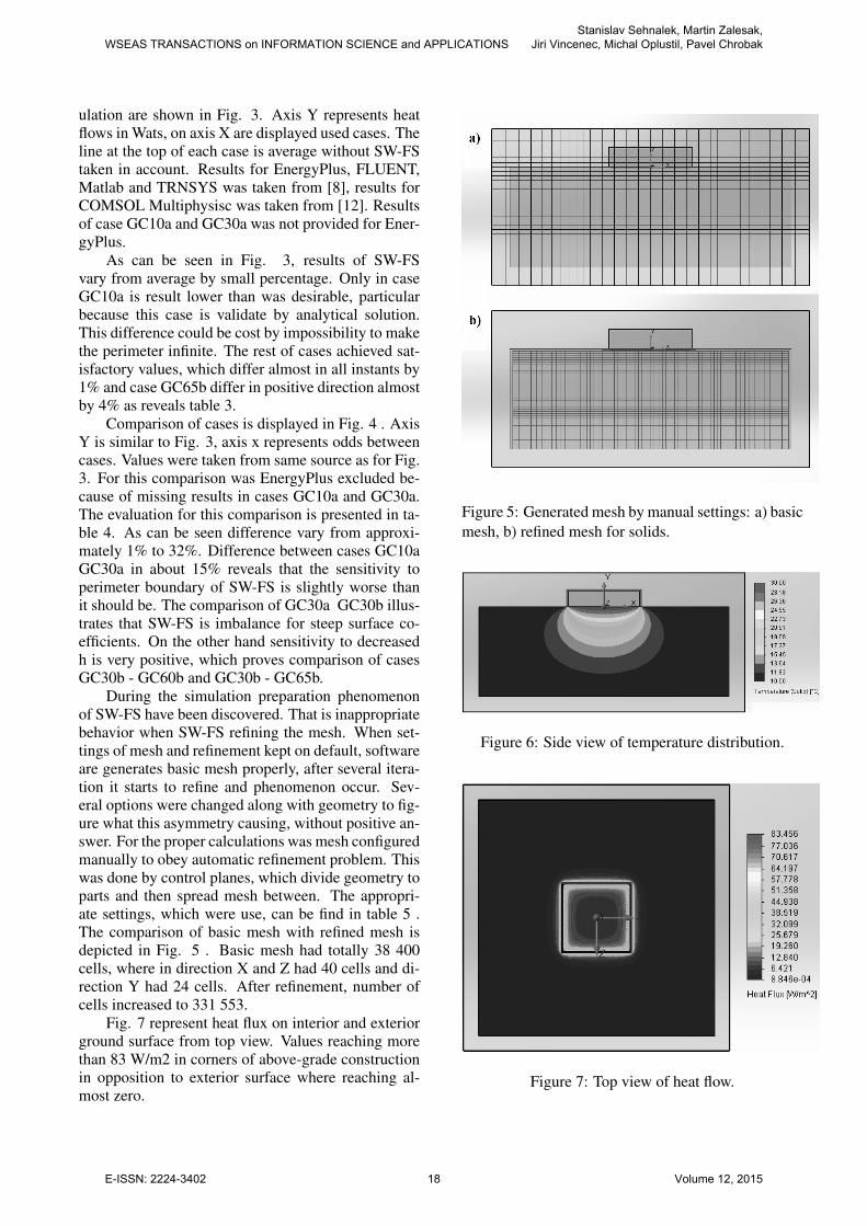
During the simulation preparation phenomenonof SW-FS have been discovered. That is inappropriatebehavior when SW-FS refining the mesh. When set-tings of mesh and refinement kept on default, softwareare generates basic mesh properly, after several itera-tion it starts to refine and phenomenon occur. Sev-eral options were changed along with geometry to fig-ure what this asymmetry causing, without positive an-swer. For the proper calculations was mesh configuredmanually to obey automatic refinement problem. Thiswas done by control planes, which divide geometry toparts and then spread mesh between. The appropri-ate settings, which were use, can be find in table 5 .The comparison of basic mesh with refined mesh isdepicted in Fig. 5 . Basic mesh had totally 38 400cells, where in direction X and Z had 40 cells and di-rection Y had 24 cells. After refinement, number ofcells increased to 331 553.

Fig. 7 represent heat flux on interior and exteriorground surface from top view. Values reaching morethan 83 W/m2 in corners of above-grade constructionin opposition to exterior surface where reaching al-most zero.

Figure 5: Generated mesh by manual settings: a) basicmesh, b) refined mesh for solids.

Figure 6: Side view of temperature distribution.

Figure 7: Top view of heat flow.



E-ISSN: 2224-3402 18 Volume 12, 2015

Table 5: Control planes settings.

Control planesin X direction

Name Minimum MaximumX1 -23,7 -10X2 -10 10X3 10 23,7

Control planesin Y direction

Name Minimum MaximumY1 -17,7 -10Y2 -10 -3Y3 -3 0Y4 0 5,6

Control planesin Z direction

Name Minimum MaximumZ1 -23,7 -10Z2 -10 10Z3 10 23,7

Side view of temperature distribution is disclosedin Fig. 6. This state is for case GC30b with basic con-ditions. Other cases are similar only with little differ-ences in distribution and geometry sizes. Displayedtemperature are in ◦C and vary from 10 ◦C for exte-rior to 30 ◦C for investigated slab.

3.3 Steady-periodic results

With this suite of cases refinement phenomenon wasnot enroll so mesh settings was kept on automaticoptions. Also due to enormous storage consump-tion quarter of computational domain was calculated.Symmetry in X and Z dimension was taken in action.Storage consumption for each case is summarized intable 6. From the table is clear that case GC50b con-sumed bulk of storage, while case GC40b used minoramount. There is no clear key to predict what amountof storage space will be needed for simulation beforerun.

Table 6: Summary of periodical cases.

CaseCondition

satisfaction[Year]

Storageconsumption

[GB]GC40a 19 19,4GC40b 7 17,7GC45b 12 20,7GC50b 22 143,4GC70b 8 24,9GC80b 13 49,5

GC40a GC40b GC45b GC50b* GC70b GC80bCases [-]

0

10000

20000

30000

40000

5000

15000

25000

35000

Floo

r Hea

t Flo

w [

kW /

h ]

SoftwaresEnergyPlusFLUENTMATLABTRNSysISO 13 370COMSOLSolidWorksAvarage

* Case GC50b is devidet by 10

Figure 8: IEA BESTEST Ground Coupling: In-DepthFloor Slab Steady-Harmonic Floor Conduction.

Output Requirements It is specified by IEABESTEST to run steady-periodic simulations as longas it is require to satisfy condition that last hour of theyear is less or equal by 0,1% than last hour in pre-vious year. Prospect for how many years calculationtake account until this condition was satisfy is in table6 .

Outcome of harmonic cases is revealed in Fig. 8.Axis are similar to that in steady-state part, with oneexception and that is that axis Y is in kW h due to itharmonic nature.

The sensitivity between cases is plotted in Fig. 9.Results for case GC40a was not provided for Energy-Plus and ISO 13 370. As was mentioned earlier it iscrucial to normalize floor are of GC50b. That can beaccomplished in the event that it is divided by (80 *80) * (12 * 12).

4 ConclusionThe results indicate, overall, that SW-FS is capableof mathematical simulation of heat flow through thefloor slab. Variation of 1% to 4% is very positive forsuch type of benchmark. As is documented in [8],there was variety from 9% to 55% disagreement be-tween firstly tested software with the analytical solu-tion. Afterwards improvement in software loweringthat difference to the highest value of 24%. Althoughversion of SW-FS was 2012 and in present time is ver-



E-ISSN: 2224-3402 19 Volume 12, 2015

GC45b-GC40b

GC40b-GC50b

GC40b-GC80b

Cases [-]

0

5000

10000

15000

20000

25000

2500

7500

12500

17500

22500

Floo

r Hea

t Flo

w [

kW /

h ]

SoftwaresEnergyPlusFLUENTMATLABTRNSYSISO 13 370COMSOLSolidWorksAvarage

Figure 9: IEA BESTEST Ground Coupling: In-DepthFloor Slab Steady-Harmonic Floor Conduction Sensi-tivity.

sion 2014 on the market, it would be interesting tobenchmark and compare results of that version withtested version.

However, appropriate setup of mesh should beconsidered along with proper analysis after genera-tion. Also refinement option should be acknowledgeas results showed big differences. Interest with re-finement should be also in symmetrical object whereSW-FS showed high disproportions.

The second part of results section contained si-nusoidal variation of outside temperature. Outcomeshow some surpassing variations in results. Mostlywith case GC50b where difference between SW-FSand average was 43%. This could be caused by the

Table 7: Periodical test cases calculated by SW-FS.

CaseSolid

Works[W]

Average[W]

Absolutedifference

[W]

Relativedifference

[%]GC40a 23096 22997 99 <1GC40b 22515 21989 526 2GC45b 30977 32101 1125 4GC50b 16467 28845 12378 43GC70b 16962 16877 85 <1GC80b 6306 5945 361 6

Table 8: Periodical test cases comparison calculatedby SW-FS.

CaseSolid

Works[W]

Average[W]

Absolutedifference

[W]

Relativedifference

[%]GC40a-GC30a

20481 20401 79 <1

GC40b-GC30b

20080 19477 603 3

GC45b-GC40b

8462 10112 1650 16

GC40b-GC50b

18810 15499 3312 21

GC70b-GC65b

15187 14962 225 2

GC40b-GC80b

16209 15478 164 1

fact that mesh was kept on automatic generation andwas not accordingly precise. Also the fact that it took22 years before it achieved 0.1% difference supportsthe mesh idea. The rest of cases are in less then10% variation. When it comes to sensitivity, SW-FSdemonstrate also good variation to average.

Further research should aim comprehensiveANSI/ASHRAE Standard 140, and properly validateSW-FS with it. Although, SW-FS is not mainly forbuilding applications, there is no snag why not to useit for such industry. Moreover as results prove it issuitable and in some cases more than other softwareadjusted mainly on it.

Acknowledgements: This work was supportedin frame of Internal Grant Agency of TomasBata University in Zlin, Faculty of Applied Infor-matics IGA/FAI/2014/015, IGA/FAI/2014/047,IGA/FAI/2014/050, and IGA/FAI/2014/057and under the project CEBIA-TECH NO.CZ.1.05/2.1.00/03.00089

References:

[1] Nicol, F. and Humphreys, M. (2007). Maxi-mum temperatures in European office buildingsto avoid heat discomfort, Solar Energy 81(3):295304.

[2] Butera, F. M. (2004). Glass architecture : is itsustainable ?, Passive and Low Energy Coolingfor the Built Environment, number May 2005,Santorini, pp. 161168.



E-ISSN: 2224-3402 20 Volume 12, 2015

[3] Poirazis, H. (2004). Double Skin Facades for Of-fice Buildings Literature Review, Technical re-port, Lund.

[4] Tsai, B.-j., Lin, S.-C. and Yang, W.-C.(2012). HVAC analysis of a building in-stalled shape-stabilized phase change materialplates coupling an active building envelope sys-tem, WSEAS TRANSACTIONS on HEAT andMASS TRANSFER 7(3): 7990.

[5] Chereches, M., Popovici, C. and Chereches,N.-C. (2010). Experimental and Numerical Ap-proach of the Thermal Conductivity of BuildingFacade Materials, WSEAS TRANSACTIONSon HEAT and MASS TRANSFER 5(3): 103112.

[6] Jarungthammachote, S. (2014). Entropy Gener-ation Analysis of Transient Heat Conduction ina Solid Slab with Fixed Temperature Bound-ary Conditions, WSEAS TRANSACTIONS onHEAT and MASS TRANSFER 9: 918.

[7] Lomas, K., Eppel, H., Martin, C. and Bloom-field, D. (1997). Empirical validation of buildingenergy simulation programs, Energy and Build-ings 26(3): 253275.

[8] Neymark, J. and Judkoff, R. (2008). In-DepthDiagnostic Cases for Ground Coupled HeatTransfer International Energy Agency BuildingEnergy Simulation Test and Diagnostic Method( IEA BESTEST ) In-Depth Diagnostic Casesfor Ground Coupled Heat Transfer Related toSlab-on-Grade Construction, Technical ReportSeptember 2008, NREL, Golden.

[9] Delsante, A. (1987). The Development of anHourly Thermal Simulation Program for Use inthe Australian Nationwide House Energy RatingScheme.

[10] Trethowen, H. and Delsante, A. (1998). Four-Year On-Site Measurement of Heat Flow inSlab-on-Ground Floors with Wet Soils, Thermalperformance of the exterior envelopes of build-ings VII(December): 487499.

[11] Judkoff, R. and Neymark, J. (2006). Model Val-idation and Testing : The Methodological Foun-dation of ASHRAE Standard 140, Technical re-port.

[12] Gerlich, V., Sulovska, K. and Zalesak, M.(2013). COMSOL Multiphysics validation assimulation software for heat transfer calculationin buildings: Building simulation software vali-dation, Measurement 46(6): 20032012.

[13] Das (2012b). SoliddWorks Flow Simulation2012 Technical Reference. Dassault SystemesSolidWorks Corp.

[14] Das (2012a). SoliddWorks Flow Simulation2012 Solving Engineering Problems with FlowSimulation 2012. Dassault Systemes Solid-Works Corp.

[15] Matsson, J. E. (2012). An Introduction to Solid-Works Flow Simulation 2012, Schroff Develop-ment Corporation.



E-ISSN: 2224-3402 21 Volume 12, 2015

Documents

Ground-Coupled Heat Transfer Test Cases as ranking ... · PDF fileGround-Coupled Heat Transfer Test Cases as ranking simulation software ... SolidWorks Flow Simulation, Software validation,